Quantum topology from symplectic geometryvivek/sobtalk.pdf · Quantum topology from symplectic...
85
Quantum topology from symplectic geometry Vivek Shende March 11, 2019
Transcript of Quantum topology from symplectic geometryvivek/sobtalk.pdf · Quantum topology from symplectic...
Quantum topology from symplectic geometry
Vivek Shende
March 11, 2019
Knots
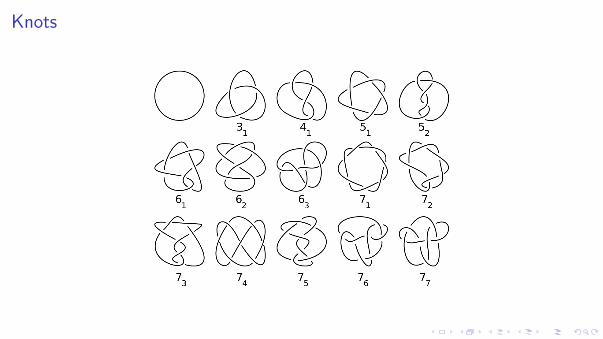
Knots
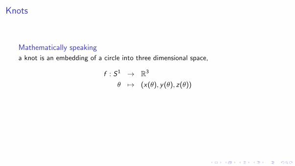
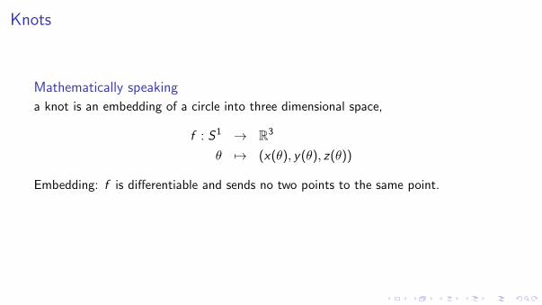
Mathematically speaking
a knot is an embedding of a circle into three dimensional space,
f : S1 → R3
θ 7→ (x(θ), y(θ), z(θ))
Embedding: f is differentiable and sends no two points to the same point.
Two knots are the sameif there is a 1-parameter family of such embeddings interpolating between them.
Knots
Mathematically speaking
a knot is an embedding of a circle into three dimensional space,
f : S1 → R3
θ 7→ (x(θ), y(θ), z(θ))
Embedding: f is differentiable and sends no two points to the same point.
Two knots are the sameif there is a 1-parameter family of such embeddings interpolating between them.
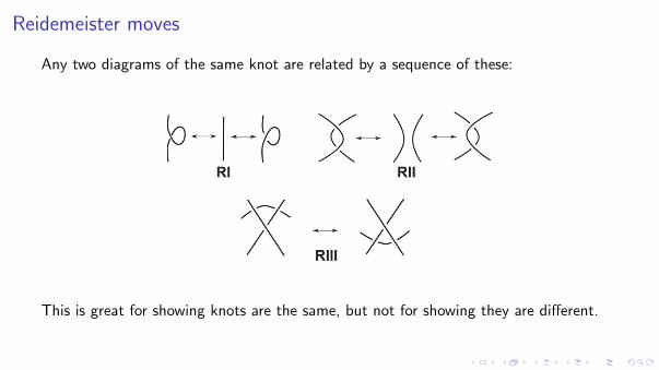
Reidemeister moves
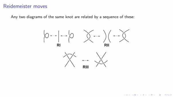
Any two diagrams of the same knot are related by a sequence of these:
This is great for showing knots are the same, but not for showing they are different.(How do you know when to give up?)
Reidemeister moves
Any two diagrams of the same knot are related by a sequence of these:
This is great for showing knots are the same, but not for showing they are different.(How do you know when to give up?)
Reidemeister moves
Any two diagrams of the same knot are related by a sequence of these:
This is great for showing knots are the same, but not for showing they are different.(How do you know when to give up?)
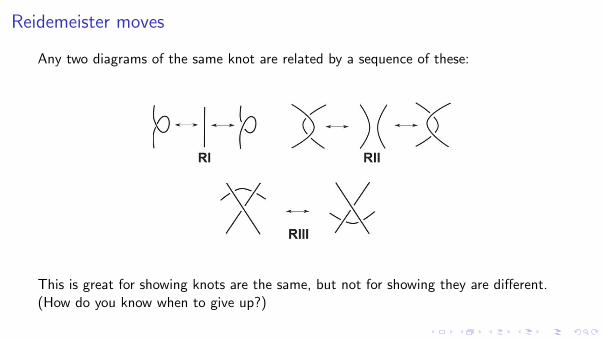
Reidemeister moves
Any two diagrams of the same knot are related by a sequence of these:
This is great for showing knots are the same, but not for showing they are different.
(How do you know when to give up?)
Reidemeister moves
Any two diagrams of the same knot are related by a sequence of these:
This is great for showing knots are the same, but not for showing they are different.(How do you know when to give up?)
How do you tell two knots apart?
Knot invariants
are rules for assigning some quantity to each knot, so that the quantity stays constantin 1-parameter families. Two knots assigned different values must be different knots!
A knot invariant is most useful when:It is computable from a knot presentation, has a geometric meaning, and takesdifferent values on different knots. These desiderata are in considerable tension.
One way to show some rule defines an invariant
Check it doesn’t change under the Reidemeister moves. This method does not usuallyclarify the geometric meaning of the invariant.
How do you tell two knots apart?
Knot invariantsare rules for assigning some quantity to each knot,
so that the quantity stays constantin 1-parameter families. Two knots assigned different values must be different knots!
A knot invariant is most useful when:It is computable from a knot presentation, has a geometric meaning, and takesdifferent values on different knots. These desiderata are in considerable tension.
One way to show some rule defines an invariant
Check it doesn’t change under the Reidemeister moves. This method does not usuallyclarify the geometric meaning of the invariant.
How do you tell two knots apart?
Knot invariantsare rules for assigning some quantity to each knot, so that the quantity stays constantin 1-parameter families.
Two knots assigned different values must be different knots!
A knot invariant is most useful when:It is computable from a knot presentation, has a geometric meaning, and takesdifferent values on different knots. These desiderata are in considerable tension.
One way to show some rule defines an invariant
Check it doesn’t change under the Reidemeister moves. This method does not usuallyclarify the geometric meaning of the invariant.
How do you tell two knots apart?
Knot invariantsare rules for assigning some quantity to each knot, so that the quantity stays constantin 1-parameter families. Two knots assigned different values must be different knots!
A knot invariant is most useful when:
It is computable from a knot presentation, has a geometric meaning, and takesdifferent values on different knots. These desiderata are in considerable tension.
One way to show some rule defines an invariant
Check it doesn’t change under the Reidemeister moves. This method does not usuallyclarify the geometric meaning of the invariant.
How do you tell two knots apart?
Knot invariantsare rules for assigning some quantity to each knot, so that the quantity stays constantin 1-parameter families. Two knots assigned different values must be different knots!
A knot invariant is most useful when:It is computable from a knot presentation,
has a geometric meaning, and takesdifferent values on different knots. These desiderata are in considerable tension.
One way to show some rule defines an invariant
Check it doesn’t change under the Reidemeister moves. This method does not usuallyclarify the geometric meaning of the invariant.
How do you tell two knots apart?
Knot invariantsare rules for assigning some quantity to each knot, so that the quantity stays constantin 1-parameter families. Two knots assigned different values must be different knots!
A knot invariant is most useful when:It is computable from a knot presentation, has a geometric meaning,
and takesdifferent values on different knots. These desiderata are in considerable tension.
One way to show some rule defines an invariant
Check it doesn’t change under the Reidemeister moves. This method does not usuallyclarify the geometric meaning of the invariant.
How do you tell two knots apart?
Knot invariantsare rules for assigning some quantity to each knot, so that the quantity stays constantin 1-parameter families. Two knots assigned different values must be different knots!
A knot invariant is most useful when:It is computable from a knot presentation, has a geometric meaning, and takesdifferent values on different knots.
These desiderata are in considerable tension.
One way to show some rule defines an invariant
Check it doesn’t change under the Reidemeister moves. This method does not usuallyclarify the geometric meaning of the invariant.
How do you tell two knots apart?
Knot invariantsare rules for assigning some quantity to each knot, so that the quantity stays constantin 1-parameter families. Two knots assigned different values must be different knots!
A knot invariant is most useful when:It is computable from a knot presentation, has a geometric meaning, and takesdifferent values on different knots. These desiderata are in considerable tension.
One way to show some rule defines an invariant
Check it doesn’t change under the Reidemeister moves. This method does not usuallyclarify the geometric meaning of the invariant.
How do you tell two knots apart?
Knot invariantsare rules for assigning some quantity to each knot, so that the quantity stays constantin 1-parameter families. Two knots assigned different values must be different knots!
A knot invariant is most useful when:It is computable from a knot presentation, has a geometric meaning, and takesdifferent values on different knots. These desiderata are in considerable tension.
One way to show some rule defines an invariant
Check it doesn’t change under the Reidemeister moves.
This method does not usuallyclarify the geometric meaning of the invariant.
How do you tell two knots apart?
Knot invariantsare rules for assigning some quantity to each knot, so that the quantity stays constantin 1-parameter families. Two knots assigned different values must be different knots!
A knot invariant is most useful when:It is computable from a knot presentation, has a geometric meaning, and takesdifferent values on different knots. These desiderata are in considerable tension.
One way to show some rule defines an invariant
Check it doesn’t change under the Reidemeister moves. This method does not usuallyclarify the geometric meaning of the invariant.

Gauss’s linking number (1833)
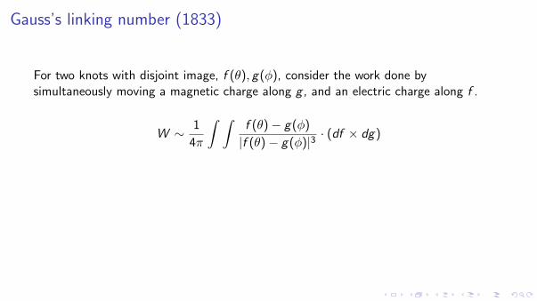
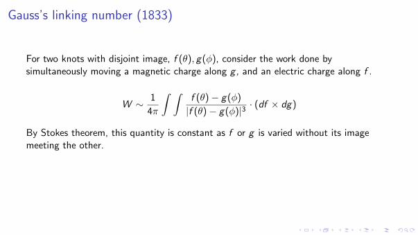
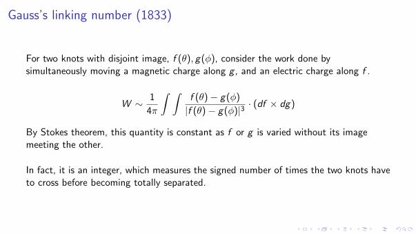
For two knots with disjoint image, f (θ), g(φ), consider the work done bysimultaneously moving a magnetic charge along g , and an electric charge along f .
W ∼ 1
4π
∫ ∫f (θ)− g(φ)
|f (θ)− g(φ)|3· (df × dg)
By Stokes theorem, this quantity is constant as f or g is varied without its imagemeeting the other.
In fact, it is an integer, which measures the signed number of times the two knots haveto cross before becoming totally separated.
Gauss’s linking number (1833)
For two knots with disjoint image, f (θ), g(φ),
consider the work done bysimultaneously moving a magnetic charge along g , and an electric charge along f .
W ∼ 1
4π
∫ ∫f (θ)− g(φ)
|f (θ)− g(φ)|3· (df × dg)
By Stokes theorem, this quantity is constant as f or g is varied without its imagemeeting the other.
In fact, it is an integer, which measures the signed number of times the two knots haveto cross before becoming totally separated.
Gauss’s linking number (1833)
For two knots with disjoint image, f (θ), g(φ), consider the work done bysimultaneously moving a magnetic charge along g , and an electric charge along f .
W ∼ 1
4π
∫ ∫f (θ)− g(φ)
|f (θ)− g(φ)|3· (df × dg)
By Stokes theorem, this quantity is constant as f or g is varied without its imagemeeting the other.
In fact, it is an integer, which measures the signed number of times the two knots haveto cross before becoming totally separated.
Gauss’s linking number (1833)
For two knots with disjoint image, f (θ), g(φ), consider the work done bysimultaneously moving a magnetic charge along g , and an electric charge along f .
W ∼ 1
4π
∫ ∫f (θ)− g(φ)
|f (θ)− g(φ)|3· (df × dg)
By Stokes theorem, this quantity is constant as f or g is varied without its imagemeeting the other.
In fact, it is an integer, which measures the signed number of times the two knots haveto cross before becoming totally separated.
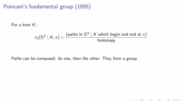
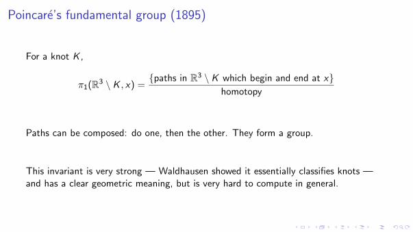
Poincare’s fundamental group (1895)
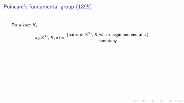
For a knot K ,
π1(R3 \ K , x) ={paths in R3 \ K which begin and end at x}
homotopy
Paths can be composed: do one, then the other. They form a group.
This invariant is very strong — Waldhausen showed it essentially classifies knots —and has a clear geometric meaning, but is very hard to compute in general.
Poincare’s fundamental group (1895)
For a knot K ,
π1(R3 \ K , x) ={paths in R3 \ K which begin and end at x}
homotopy
Paths can be composed: do one, then the other. They form a group.
This invariant is very strong — Waldhausen showed it essentially classifies knots —and has a clear geometric meaning, but is very hard to compute in general.
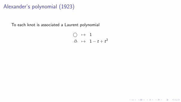
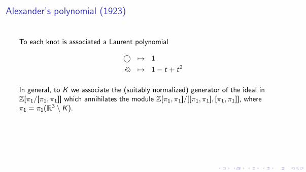
Alexander’s polynomial (1923)
To each knot is associated a Laurent polynomial
© 7→ 1
& 7→ 1− t + t2
In general, to K we associate the (suitably normalized) generator of the ideal inZ[π1/[π1, π1]] which annihilates the module Z[π1, π1]/[[π1, π1], [π1, π1]], whereπ1 = π1(R3 \ K ). (There are many other descriptions.)
Many knots other than © have Alexander polynomial 1. By Freedman’s disk theorem)any such knot bounds a locally flat disk in the 4-ball.
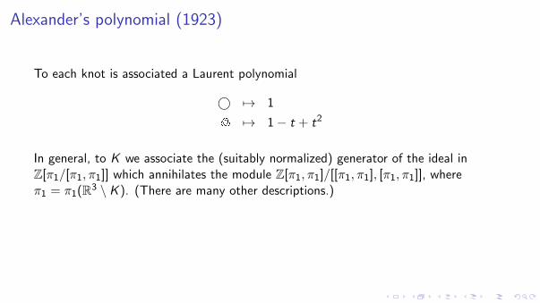
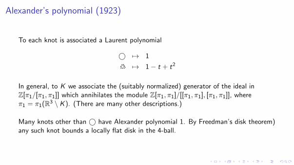
Alexander’s polynomial (1923)
To each knot is associated a Laurent polynomial
© 7→ 1
& 7→ 1− t + t2
In general, to K we associate the (suitably normalized) generator of the ideal inZ[π1/[π1, π1]] which annihilates the module Z[π1, π1]/[[π1, π1], [π1, π1]], whereπ1 = π1(R3 \ K ).
(There are many other descriptions.)
Many knots other than © have Alexander polynomial 1. By Freedman’s disk theorem)any such knot bounds a locally flat disk in the 4-ball.
Alexander’s polynomial (1923)
To each knot is associated a Laurent polynomial
© 7→ 1
& 7→ 1− t + t2
In general, to K we associate the (suitably normalized) generator of the ideal inZ[π1/[π1, π1]] which annihilates the module Z[π1, π1]/[[π1, π1], [π1, π1]], whereπ1 = π1(R3 \ K ). (There are many other descriptions.)
Many knots other than © have Alexander polynomial 1. By Freedman’s disk theorem)any such knot bounds a locally flat disk in the 4-ball.
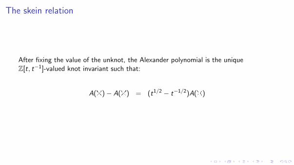
The skein relation
After fixing the value of the unknot, the Alexander polynomial is the uniqueZ[t, t−1]-valued knot invariant such that:
A(!)− A(") = (t1/2 − t−1/2)A(H)
Jones’s polynomial (1983)
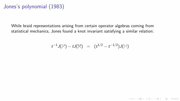
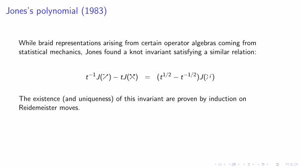
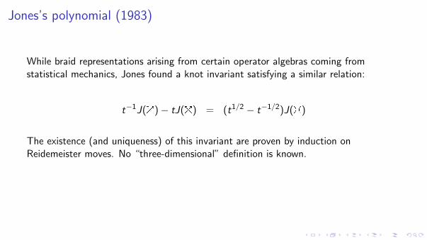
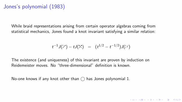
While braid representations arising from certain operator algebras coming fromstatistical mechanics, Jones found a knot invariant satisfying a similar relation:
t−1J(!)− tJ(") = (t1/2 − t−1/2)J(H)
The existence (and uniqueness) of this invariant are proven by induction onReidemeister moves. No “three-dimensional” definition is known.
No-one knows if any knot other than © has Jones polynomial 1.
Jones’s polynomial (1983)
While braid representations arising from certain operator algebras coming fromstatistical mechanics,
Jones found a knot invariant satisfying a similar relation:
t−1J(!)− tJ(") = (t1/2 − t−1/2)J(H)
The existence (and uniqueness) of this invariant are proven by induction onReidemeister moves. No “three-dimensional” definition is known.
No-one knows if any knot other than © has Jones polynomial 1.
Jones’s polynomial (1983)
While braid representations arising from certain operator algebras coming fromstatistical mechanics, Jones found a knot invariant satisfying a similar relation:
t−1J(!)− tJ(") = (t1/2 − t−1/2)J(H)
The existence (and uniqueness) of this invariant are proven by induction onReidemeister moves. No “three-dimensional” definition is known.
No-one knows if any knot other than © has Jones polynomial 1.
Jones’s polynomial (1983)
While braid representations arising from certain operator algebras coming fromstatistical mechanics, Jones found a knot invariant satisfying a similar relation:
t−1J(!)− tJ(") = (t1/2 − t−1/2)J(H)
The existence (and uniqueness) of this invariant are proven by induction onReidemeister moves.
No “three-dimensional” definition is known.
No-one knows if any knot other than © has Jones polynomial 1.
Jones’s polynomial (1983)
While braid representations arising from certain operator algebras coming fromstatistical mechanics, Jones found a knot invariant satisfying a similar relation:
t−1J(!)− tJ(") = (t1/2 − t−1/2)J(H)
The existence (and uniqueness) of this invariant are proven by induction onReidemeister moves. No “three-dimensional” definition is known.
No-one knows if any knot other than © has Jones polynomial 1.
Jones’s polynomial (1983)
While braid representations arising from certain operator algebras coming fromstatistical mechanics, Jones found a knot invariant satisfying a similar relation:
t−1J(!)− tJ(") = (t1/2 − t−1/2)J(H)
The existence (and uniqueness) of this invariant are proven by induction onReidemeister moves. No “three-dimensional” definition is known.
No-one knows if any knot other than © has Jones polynomial 1.
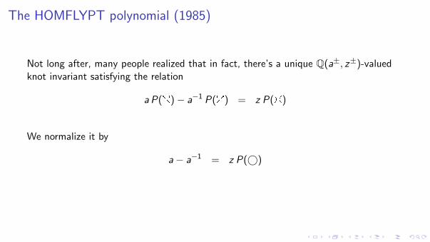
The HOMFLYPT polynomial (1985)
Not long after, many people realized that in fact, there’s a unique Q(a±, z±)-valuedknot invariant satisfying the relation
a P(!)− a−1 P(") = z P(H)
We normalize it by
a− a−1 = z P(©)

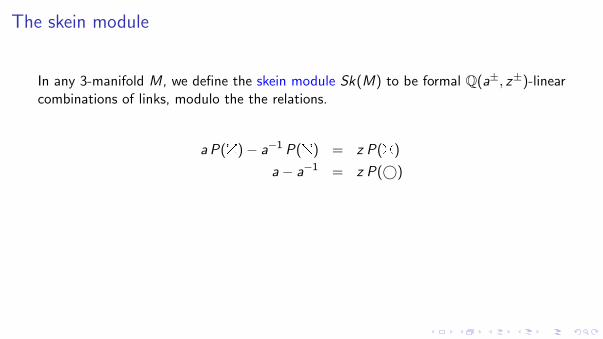
The skein module
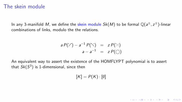
In any 3-manifold M, we define the skein module Sk(M) to be formal Q(a±, z±)-linearcombinations of links, modulo the the relations.
a P(!)− a−1 P(") = z P(H)
a− a−1 = z P(©)
An equivalent way to assert the existence of the HOMFLYPT polynomial is to assertthat Sk(S3) is 1-dimensional, since then
[K ] = P(K ) · [∅]
The skein module
In any 3-manifold M, we define the skein module Sk(M) to be formal Q(a±, z±)-linearcombinations of links, modulo the the relations.
a P(!)− a−1 P(") = z P(H)
a− a−1 = z P(©)
An equivalent way to assert the existence of the HOMFLYPT polynomial is to assertthat Sk(S3) is 1-dimensional, since then
[K ] = P(K ) · [∅]
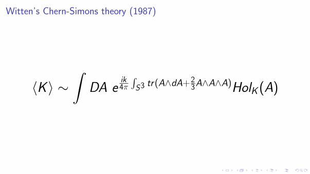
Witten’s Chern-Simons theory (1987)
〈K 〉 ∼∫
DA eik4π
∫S3 tr(A∧dA+2
3A∧A∧A)HolK(A)
One way we learn geometry from physics
Physical systems may depend on parameters, yet have some quantities which areconserved as parameters vary.
Different limits may have different geometric descriptions — e.g., some of thegeometry may collapse or decouple.
In each limit, some quantities may have geometric intepretations. If these quantitiesare conserved, then we discover they have two different geometric interpretations.
The physical arguments may have not been mathematically rigorous (e.g. because wedo not know how to define the Feynman integral), the resulting statement is oftenmathematically precise – though still conjectural.
One way we learn geometry from physics
Physical systems may depend on parameters, yet have some quantities which areconserved as parameters vary.
Different limits may have different geometric descriptions — e.g., some of thegeometry may collapse or decouple.
In each limit, some quantities may have geometric intepretations.
If these quantitiesare conserved, then we discover they have two different geometric interpretations.
The physical arguments may have not been mathematically rigorous (e.g. because wedo not know how to define the Feynman integral), the resulting statement is oftenmathematically precise – though still conjectural.
One way we learn geometry from physics
Physical systems may depend on parameters, yet have some quantities which areconserved as parameters vary.
Different limits may have different geometric descriptions — e.g., some of thegeometry may collapse or decouple.
In each limit, some quantities may have geometric intepretations. If these quantitiesare conserved, then we discover they have two different geometric interpretations.
The physical arguments may have not been mathematically rigorous (e.g. because wedo not know how to define the Feynman integral), the resulting statement is oftenmathematically precise – though still conjectural.
One way we learn geometry from physics
Physical systems may depend on parameters, yet have some quantities which areconserved as parameters vary.
Different limits may have different geometric descriptions — e.g., some of thegeometry may collapse or decouple.
In each limit, some quantities may have geometric intepretations. If these quantitiesare conserved, then we discover they have two different geometric interpretations.
The physical arguments may have not been mathematically rigorous (e.g. because wedo not know how to define the Feynman integral), the resulting statement is oftenmathematically precise – though still conjectural.
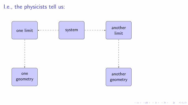
I.e., the physicists tell us:
systemone limitanother
limit
onegeometry
anothergeometry
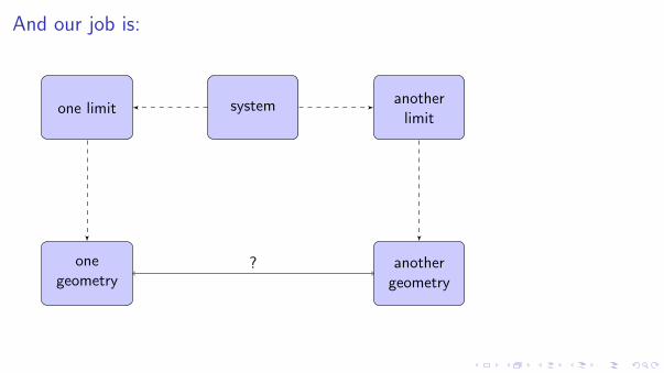
And our job is:
systemone limitanother
limit
onegeometry
anothergeometry
?
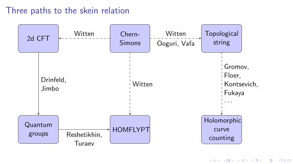
Three paths to the skein relation
Chern-Simons
2d CFT
Quantumgroups
HOMFLYPT
Topologicalstring
Holomorphiccurve
counting
Witten
Ooguri, Vafa
Witten
Witten
Drinfeld,Jimbo
Reshetikhin,Turaev
Gromov,Floer,Kontsevich,Fukaya· · ·
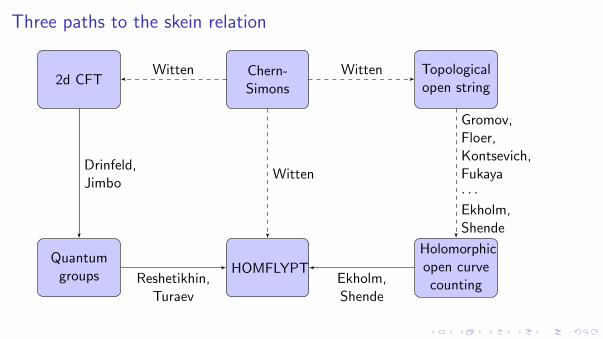
Three paths to the skein relation
Chern-Simons
2d CFT
Quantumgroups
HOMFLYPT
Topologicalopen string
Holomorphicopen curvecounting
Witten
Witten
Witten
Drinfeld,Jimbo
Reshetikhin,Turaev
Gromov,Floer,Kontsevich,Fukaya· · ·Ekholm,Shende
Ekholm,Shende
J-holomorphic maps: local theory
If (X , J) is an almost complex manifold, and (C , j) is a Riemann surface, we can askfor a map f : C → X satisfying df ◦ j = J ◦ df .
This is a nonlinear elliptic PDE. Its linearization is Fredholm with index computed byRiemann-Roch to be 2
(∫C f ∗c1(M) + (3− d)(1− g)
).
In an ideal world, the index is the dimension of the space of deformations of such maps.
In the real world, we perturb the equation to make this true.
The index vanishes when M is a Calabi-Yau manifold (c1(M) = 0) of complexdimension d = 3.
J-holomorphic maps: global theory
When there’s a symplectic form ω so that g = ω(· , J · ) is a metric, then the quantity
I =
∫Cf ∗ω
is both topological (because ω is closed) and is the g -area of f (C ).
Using this control, Gromov classified how families of such maps may degenerate, andshowed that after allowing certain explicit bubbling behaviors, the space of solutionsbecomes compact (after fixing topological data).
Gromov-Witten invariants of Calabi-Yau 3-folds
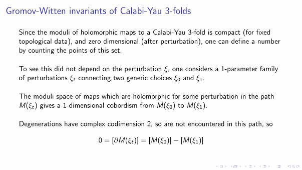
Since the moduli of holomorphic maps to a Calabi-Yau 3-fold is compact (for fixedtopological data), and zero dimensional (after perturbation), one can define a numberby counting the points of this set.
To see this did not depend on the perturbation ξ, one considers a 1-parameter familyof perturbations ξt connecting two generic choices ξ0 and ξ1.
The moduli space of maps which are holomorphic for some perturbation in the pathM(ξt) gives a 1-dimensional cobordism from M(ξ0) to M(ξ1).
Degenerations have complex codimension 2, so are not encountered in this path, so
0 = [∂M(ξt)] = [M(ξ0)]− [M(ξ1)]
Gromov-Witten invariants of Calabi-Yau 3-folds
Since the moduli of holomorphic maps to a Calabi-Yau 3-fold is compact (for fixedtopological data), and zero dimensional (after perturbation), one can define a numberby counting the points of this set.
To see this did not depend on the perturbation ξ, one considers a 1-parameter familyof perturbations ξt connecting two generic choices ξ0 and ξ1.
The moduli space of maps which are holomorphic for some perturbation in the pathM(ξt) gives a 1-dimensional cobordism from M(ξ0) to M(ξ1).
Degenerations have complex codimension 2, so are not encountered in this path, so
0 = [∂M(ξt)] = [M(ξ0)]− [M(ξ1)]
Open Gromov-Witten invariants?
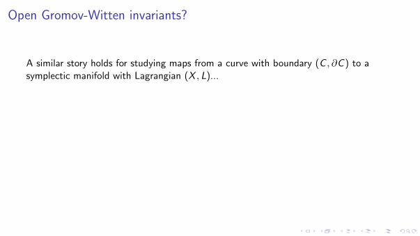
A similar story holds for studying maps from a curve with boundary (C , ∂C ) to asymplectic manifold with Lagrangian (X , L)...
except that ∂M(ξt) has other components.
This is because there is a 1-real parameter space of choices to smooth a boundarydegeneration, as compared to a 1-complex parameter space of choices to smooth aninterior one.
Naively, this seems to mean the corresponding count is not well defined.

Open Gromov-Witten invariants?
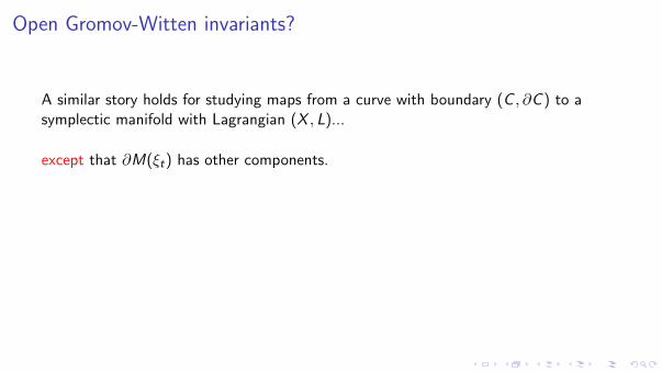
A similar story holds for studying maps from a curve with boundary (C , ∂C ) to asymplectic manifold with Lagrangian (X , L)...
except that ∂M(ξt) has other components.
This is because there is a 1-real parameter space of choices to smooth a boundarydegeneration, as compared to a 1-complex parameter space of choices to smooth aninterior one.
Naively, this seems to mean the corresponding count is not well defined.
Open Gromov-Witten invariants?
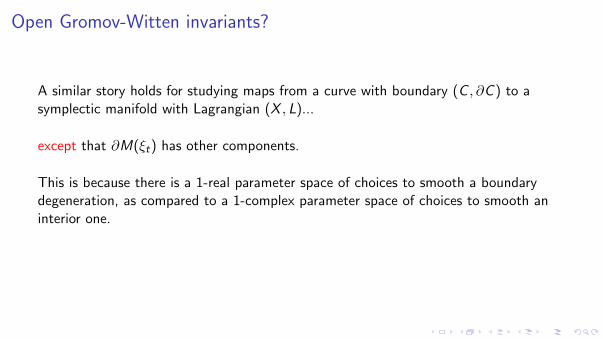
A similar story holds for studying maps from a curve with boundary (C , ∂C ) to asymplectic manifold with Lagrangian (X , L)...
except that ∂M(ξt) has other components.
This is because there is a 1-real parameter space of choices to smooth a boundarydegeneration, as compared to a 1-complex parameter space of choices to smooth aninterior one.
Naively, this seems to mean the corresponding count is not well defined.
Open Gromov-Witten invariants?
A similar story holds for studying maps from a curve with boundary (C , ∂C ) to asymplectic manifold with Lagrangian (X , L)...
except that ∂M(ξt) has other components.
This is because there is a 1-real parameter space of choices to smooth a boundarydegeneration, as compared to a 1-complex parameter space of choices to smooth aninterior one.
Naively, this seems to mean the corresponding count is not well defined.
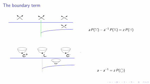
The boundary term
C CL+ -
a P(!)− a−1 P(") = z P(H)
a− a−1 = z P(©)
Open Gromov-Witten invariants
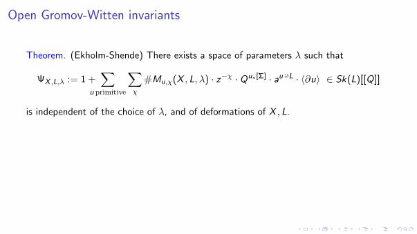
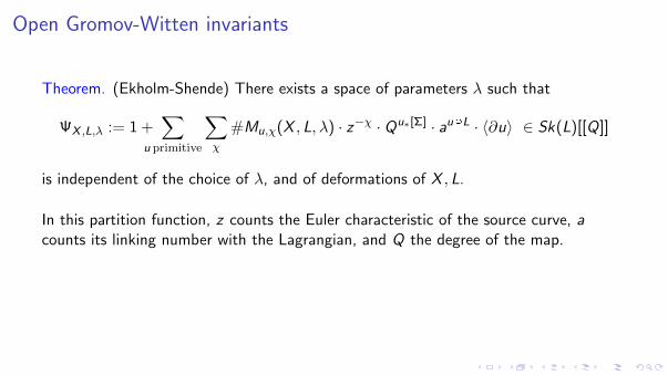
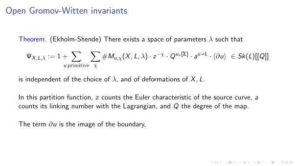
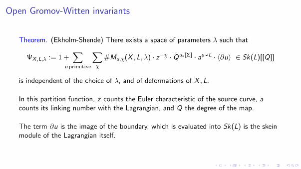
Theorem. (Ekholm-Shende) There exists a space of parameters λ such that
ΨX ,L,λ := 1 +∑
u primitive
∑χ
#Mu,χ(X , L, λ) · z−χ · Qu∗[Σ] · auAL · 〈∂u〉 ∈ Sk(L)[[Q]]
is independent of the choice of λ, and of deformations of X , L.
In this partition function, z counts the Euler characteristic of the source curve, acounts its linking number with the Lagrangian, and Q the degree of the map.
The term ∂u is the image of the boundary, which is evaluated into Sk(L) is the skeinmodule of the Lagrangian itself.
Open Gromov-Witten invariants
Theorem. (Ekholm-Shende) There exists a space of parameters λ such that
ΨX ,L,λ := 1 +∑
u primitive
∑χ
#Mu,χ(X , L, λ) · z−χ · Qu∗[Σ] · auAL · 〈∂u〉 ∈ Sk(L)[[Q]]
is independent of the choice of λ, and of deformations of X , L.
In this partition function, z counts the Euler characteristic of the source curve, acounts its linking number with the Lagrangian, and Q the degree of the map.
The term ∂u is the image of the boundary,
which is evaluated into Sk(L) is the skeinmodule of the Lagrangian itself.
Open Gromov-Witten invariants
Theorem. (Ekholm-Shende) There exists a space of parameters λ such that
ΨX ,L,λ := 1 +∑
u primitive
∑χ
#Mu,χ(X , L, λ) · z−χ · Qu∗[Σ] · auAL · 〈∂u〉 ∈ Sk(L)[[Q]]
is independent of the choice of λ, and of deformations of X , L.
In this partition function, z counts the Euler characteristic of the source curve, acounts its linking number with the Lagrangian, and Q the degree of the map.
The term ∂u is the image of the boundary, which is evaluated into Sk(L) is the skeinmodule of the Lagrangian itself.
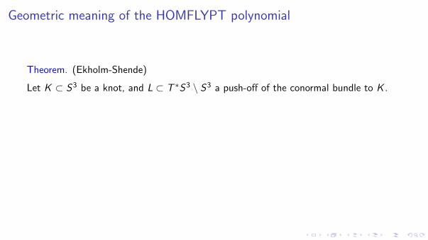
Geometric meaning of the HOMFLYPT polynomial
Theorem. (Ekholm-Shende)
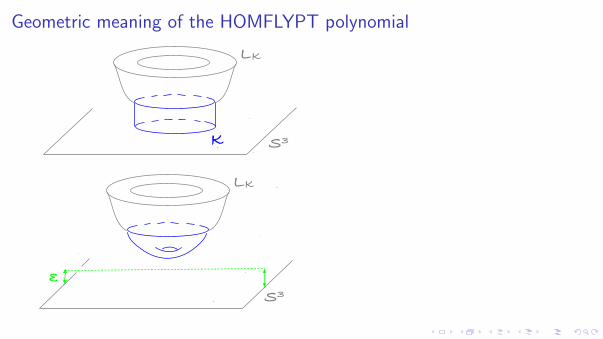
Let K ⊂ S3 be a knot, and L ⊂ T ∗S3 \ S3 a push-off of the conormal bundle to K .
Then the degree 1 term of ΨT∗S3\S3,L is the HOMFLYPT polynomial of K .
This (makes sense of and) confirms a prediction of Ooguri and Vafa.
Geometric meaning of the HOMFLYPT polynomial
Theorem. (Ekholm-Shende)
Let K ⊂ S3 be a knot, and L ⊂ T ∗S3 \ S3 a push-off of the conormal bundle to K .
Then the degree 1 term of ΨT∗S3\S3,L is the HOMFLYPT polynomial of K .
This (makes sense of and) confirms a prediction of Ooguri and Vafa.
Geometric meaning of the HOMFLYPT polynomial
Theorem. (Ekholm-Shende)
Let K ⊂ S3 be a knot, and L ⊂ T ∗S3 \ S3 a push-off of the conormal bundle to K .
Then the degree 1 term of ΨT∗S3\S3,L is the HOMFLYPT polynomial of K .
This (makes sense of and) confirms a prediction of Ooguri and Vafa.
Geometric meaning of the HOMFLYPT polynomial
LK
LK
S3ε
S3K
![Symplectic maps to projective spaces and symplectic invariants · AUROUX Theorem 2.1 (Donaldson [10]). For k˛0, two suitably chosen approximately holomor- phic sections of L⊗k](https://static.fdocument.org/doc/165x107/6071f9ebb95cf304647f3cb8/symplectic-maps-to-projective-spaces-and-symplectic-invariants-auroux-theorem-21.jpg)