An Introduction to Non Perturbative RGor ERG or FRG or eRG

Bertrand Delamotte, LPTMC, Universite Paris VI

Corfu, September 2010

ERG10

Some basic notions on Statistical Field Theory

Ising (or Heisenberg) model and the φ4 theory:– on the lattice:

Z[B] =∑

{Si =±1}

exp{− βJ

∑<ij>

SiSj + β∑

i

BiSi

}– in the continuum (keeping only the leading derivative term):

Z[J] =

∫Dφ exp

{− S[φ] +

∫x

J(x)φ(x)}

with (a = lattice spacing)

S[φ] =

∫ddx

{1

2

(∇φ)2

+ da−2φ2 − a−d ln(

cosh(β

√4Jd2

βa2−dφ))}

Making a field expansion leads to:

S =

∫ddx

{1

2

(∇φ)2

+m2

0

2φ2 +

g0

4!φ4 + . . .

}ERG10

The physical quantities we are interested in:

– “thermodynamic quantities”:

magnetization (classical field, vev,...) : M = 〈φ〉 = 1Z∂Z∂B

susceptibility (response of M to a change of B) : χ = ∂M∂B

correlation length ξ (renormalized mass)

critical temperature Tc and phase diagram

etc

– correlation function(s): 〈SiSj〉 ∼ 〈φ(x)φ(y)〉 = G (2)(x , y)and G (n)(x1, . . . , xn)

⇒ universal and non-universal quantities.

ERG10

The theoretical tools and methods:

– The generating functional of correlation functions:

Z[J], W[J] = lnZ[J] and Γ[M] = Legendre transform of W[J]:

Γ[M] +W[J] =

∫x

JxMx

⇒ Mx = 〈φx〉 =δW[J]

δJxand Jx =

δΓ[M]

δMx

– The mean field (classical, saddle point, Hartree) approximation:

Γ[M]→ ΓMF[M] = S[φ = M]

neglects all fluctuations around the mean field configuration M.

ERG10

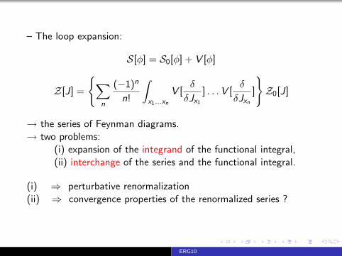
– The loop expansion:

S[φ] = S0[φ] + V [φ]

Z[J] =

{∑n

(−1)n

n!

∫x1...xn

V [δ

δJx1

] . . .V [δ

δJxn

]

}Z0[J]

→ the series of Feynman diagrams.→ two problems:

(i) expansion of the integrand of the functional integral,(ii) interchange of the series and the functional integral.

(i) ⇒ perturbative renormalization(ii) ⇒ convergence properties of the renormalized series ?

ERG10

Why should we be interested in NPRG?

Perturbation theory works well when:

g is small: QED;

g is not small, the renormalized series is Borel-summable andenough terms are known: φ4 in d = 3.

Perturbation theory doesn’t work well when:

g is not small and not enough terms are known;

g is not small, the series is Borel-summable, convergence to awrong result: φ4 in d = 2: η = 0.145(14) instead of 0.25;

g is not small and the series cannot be resummed: O(N)non-linear-sigma model in d = 2 + ε;

infinitely many couplings have to be taken care: computationof Tc ;

the phenomenon is genuinely non-perturbative: no RGtrajectory Gaussian → fixed point, convexity of the effectivepotential.

ERG10

Wilson RG:

Organize the summation over the fluctuations in a different way.⇓

Block-spins a la Kadanoff-Wilson⇓

summation over rapid modes → effective hamiltonian for the slow modes⇓

flow equations of functions (or even functionals)

Two main implementations of these ideas:

a la Wilson-Polchinski (flow of actions or of W[J])and

a la Parola-Reatto-Wetterich (flow of the Legendre transformΓ[M]).

In principle equivalent, but...

ERG10

Integration over the rapid modes:

hypothesis: the system is close to criticality (ξ � a ⇒ mR � Λ)

integrate over the rapid modes only → freeze the slow modes→ make them non-critical → give them a large mass

q

Rk HqL

k

k2

ERG10

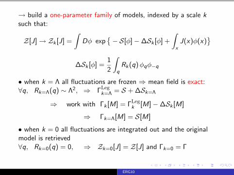
→ build a one-parameter family of models, indexed by a scale ksuch that:

Z[J]→ Zk [J] =

∫Dφ exp

{− S[φ]−∆Sk [φ] +

∫x

J(x)φ(x)}

∆Sk [φ] =1

2

∫q

Rk(q)φqφ−q

• when k = Λ all fluctuations are frozen ⇒ mean field is exact:∀q, Rk=Λ(q) ∼ Λ2, ⇒ ΓLeg

k=Λ = S + ∆Sk=Λ

⇒ work with Γk [M] = ΓLegk [M]−∆Sk [M]

⇒ Γk=Λ[M] = S[M]

• when k = 0 all fluctuations are integrated out and the originalmodel is retrieved∀q, Rk=0(q) = 0, ⇒ Zk=0[J] = Z[J] and Γk=0 = Γ

ERG10

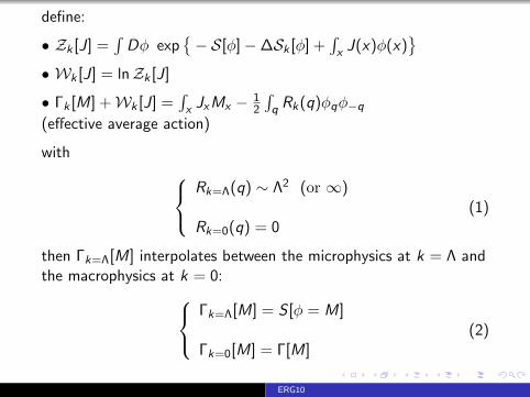
define:

• Zk [J] =∫

Dφ exp{− S[φ]−∆Sk [φ] +

∫x J(x)φ(x)

}• Wk [J] = lnZk [J]

• Γk [M] +Wk [J] =∫x JxMx − 1

2

∫q Rk(q)φqφ−q

(effective average action)

with Rk=Λ(q) ∼ Λ2 (or ∞)

Rk=0(q) = 0(1)

then Γk=Λ[M] interpolates between the microphysics at k = Λ andthe macrophysics at k = 0:

Γk=Λ[M] = S [φ = M]

Γk=0[M] = Γ[M](2)

ERG10

The flow equation for Γk [M] writes:

∂kΓk [M] =1

2

∫q∂kRk(q)G [q; M] (3)

where G [q; M] is the full propagator: G [q; M] = (Γ(2)k + Rk)−1

Some properties of the Wetterich’s equation:– differential formulation of field theory– involves only one integral– the initial condition is the (microscopic) bare theory– good properties of decoupling of the massive and rapid modes– starting point of non-perturbative approximation schemes (notlinked to an expansion in a small parameter)

– BUT leads to very few exact results.

ERG10

Approximation schemes require

to lead to tractable calculations;

to focus on the “sector” of the model that we want todescribe;

to preserve automatically the good properties of RG;

to enable a systematic improvement of the results.

Two main (non-perturbative) approximation schemes:The derivative expansion (DE)The Blaizot-Mendez-Wschebor scheme (BMW)

ERG10

The derivative expansion

Γk =∫

ddx(Uk(M) + 1

2 Zk(M)(∇M)2 + O(∇4))

flow of Γk ⇒ flow of Uk(M),Zk(M), ...

Consists in keeping all Γ(n)k correlation functions and expanding in

their momenta (more precisely in pik ).

Most celebrated: Local Potential Approximation (LPA):

Γ LPAk =

∫ddx

(Uk(M) +

1

2(∇M)2

)- bare momentum dependence of Γ

(2)k (p);

- zero momentum approximation for all other correlation functions.

∂kUk(M) =kd+1

k2 + U ′′k (M)

ERG10

Some properties of the DE (for the O(N) models)

– it is one-loop exact in d = 4− ε and in d = 2 + ε (for N ≥ 2)and exact for U = Uk=0 at N =∞ (LPA’)– it preserves the convexity of U = Uk=0 in the broken phase (LPA)– initial conditions ⇒ non-universal physics ⇒ computation of Tc

– it reproduces well the physics of the Kosterlitz-Thoulesstransition (N = 2, d = 2)– it leads to accurate results for the universal quantities: Isingmodel in d = 3:NPRG: ν = 0.63014 η = 0.0352Monte Carlo: ν = 0.63020(12) η = 0.368(2)6 loops: ν = 0.6304(13) η = 0.335(25)

ERG10

But the DE has some drawbacks:

(i) the physical quantities depend on the choice of Rk ;

(ii) the momentum dependence of the Γ(n)k ({pi},M = 0) is badly

truncated: at Tc (that is mR = 0): Γ(2)k=0(p) ∼ p2−η.

(i) ⇒ does the DE converge?(ii) ⇒ for which pi is the DE valid?

ERG10

Does the DE converge?

No general answer.

Test:

convergence ⇒ dependence upon Rk decreases with the order.

But this is an ill-posed problem!

ERG10

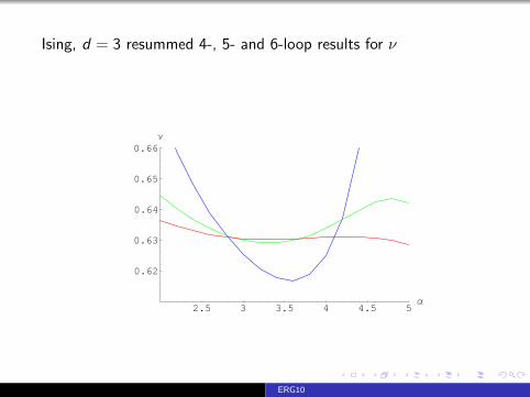
Ising, d = 3 resummed 4-, 5- and 6-loop results for ν

2.5 3 3.5 4 4.5 5Α

0.62

0.63

0.64

0.65

0.66Ν

ERG10

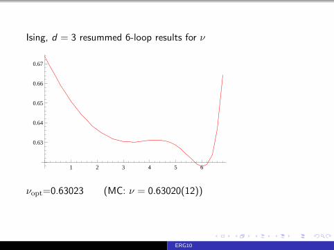
Ising, d = 3 resummed 6-loop results for ν

1 2 3 4 5 6

0.63

0.64

0.65

0.66

0.67

νopt=0.63023 (MC: ν = 0.63020(12))

ERG10

0 1 2 3 4order

0.6250.6300.6350.6400.6450.650

Ν

0 1 2 3 4order

0.02

0.04

0.06

0.08

0.10

Η

ERG10

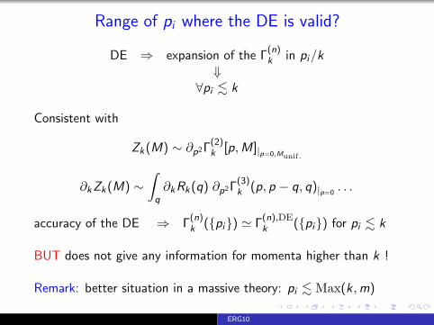
Range of pi where the DE is valid?

DE ⇒ expansion of the Γ(n)k in pi/k

⇓∀pi . k

Consistent with

Zk(M) ∼ ∂p2Γ(2)k [p,M]|p=0,Munif.

∂kZk(M) ∼∫

q∂kRk(q) ∂p2Γ

(3)k (p, p − q, q)|p=0

. . .

accuracy of the DE ⇒ Γ(n)k ({pi}) ' Γ

(n),DEk ({pi}) for pi . k

BUT does not give any information for momenta higher than k !

Remark: better situation in a massive theory: pi . Max(k,m)

ERG10

Blaizot-Mendez-Wschebor (BMW) approximation

keep all Γ(n)k correlation functions (as in the DE);

aim at being as accurate as possible for the Γ(n)k ’s with low n;

Exact equation on Γ(2)k (p,M) (for uniform field M):

∂kΓ(2)k (p,M) =

∫q∂kRk(q)G (q; M)2

(− 1

2Γ

(4)k (p,−p, q,−q; M)

+ Γ(3)k (p, q,−p − q; M)G (p + q; M)Γ

(3)k (−p,−q, p + q; M)

)Infinite hierarchy of equations on the Γ

(n)k ({pi},M)

⇒ closure requires approx. on Γ(3)k and Γ

(4)k in terms of Γ

(2)k

truncate the momentum dependence of the Γ(n)k ’s with

“large” n ⇒ closed set of equations for Γ(n)k with low n.

First order: LPA, already good for p → 0 in many cases.

Second order: keep Γ(2)k , truncate Γ

(3)k , Γ

(4)k , ...

ERG10

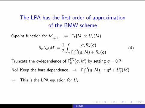
The LPA has the first order of approximation

of the BMW scheme

0-point function for M|unif.⇒ Γk [M] ∝ Uk(M)

∂kUk(M) =1

2

∫q

∂kRk(q)

Γ(2)k (q,M) + Rk(q)

(4)

Truncate the q-dependence of Γ(2)k (q,M) by setting q = 0 ?

No! Keep the bare dependence ⇒ Γ(2)k (q,M)→ q2 + U ′′k (M)

⇒ This is the LPA equation for Uk .

ERG10

The second order of approximation of BMW

∂kΓ(2)k (p; M) =

∫q∂kRk(q)G (q; M)2

(− 1

2Γ

(4)k (p,−p, q,−q; M)

+Γ(3)k (p, q,−p − q; M)G (p + q; M)Γ

(3)k (−p,−q, p + q; M)

)Three (crucial) remarks

q . k because of Rk(q);

finite k ⇒ no IR divergence ⇒ Γ(n)k ({pi},M) expandable in pi ;

Γ(n)k (p1, . . . , pn−1, 0; M) =

∂

∂MΓ

(n−1)k (p1, . . . , pn−1; M).

Thus

for p � k > q ⇒ Γ(3)k (p, q,−p − q; M) ' Γ

(3)k (p, 0,−p; M)

and Γ(4)k (p,−p, q,−q; M) ' Γ

(4)k (p,−p, 0, 0; M)

for p � k:“LPA regime”: again q is neglected and p → 0

ERG10

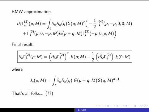
BMW approximation

∂kΓ(2)k (p; M) =

∫q∂kRk(q)G (q; M)2

(− 1

2Γ

(4)k (p,−p, 0, 0; M)

+ Γ(3)k (p, 0,−p; M)G (p + q; M)Γ

(3)k (−p, 0, p; M)

)Final result:

∂kΓ(2)k (p; M) =

(∂MΓ

(2)k

)2J3(p; M)− 1

2

(∂2

MΓ(2)k

)J2(0; M)

where

Jn(p; M) =

∫q∂kRk(q) G (p + q; M)G (q; M)n−1

That’s all folks... (??)

ERG10

Not fully !

Search for fixed points:

⇒ numerical instabilities

⇒ good variablesΓ

(2)k (p,M)− Γ

(2)k (0,M)

p2− 1 and Vk(M)

⇒ difficulties for p → 0⇒ necessary to avoid non analytic Rk functions...

Results in d = 3, N = 1:

η = 0.039 ηMC = 0.0368(2)ν = 0.632 νMC = 0.6302(1)ω = 0.78 ωMC = 0.821(5)

ERG10

Results in d = 2, N = 1:

η = 0.254 η = 0.25ν = 1.00 ν = 1

AND... at five loops: η = 0.145(14)

ERG10

ERG10

ERG10

ERG10

ERG10