KKT conditions and Duality
36
KKT conditions and Duality March 23, 2012
Transcript of KKT conditions and Duality

KKT conditions and Duality
March 23, 2012
Tutorial Example
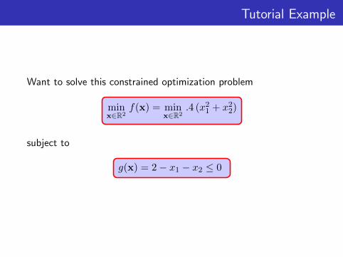
Want to solve this constrained optimization problem
minx∈R2
f(x) = minx∈R2
.4 (x21 + x22)
subject to
g(x) = 2− x1 − x2 ≤ 0
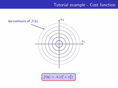
Tutorial example - Cost function
x1
x2iso-contours of f(x)
f(x) = .4 (x21 + x22)
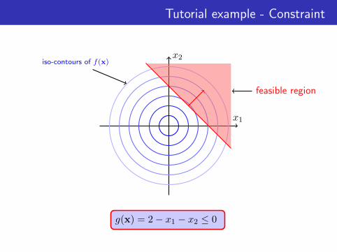
Tutorial example - Constraint
x1
x2iso-contours of f(x)
feasible region
g(x) = 2− x1 − x2 ≤ 0
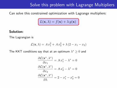
Solve this problem with Lagrange Multipliers
Can solve this constrained optimization with Lagrange multipliers:
L(x, λ) = f(x) + λ g(x)
Solution:
The Lagrangian is
L(x, λ) = .4x21 + .4x22 + λ (2− x1 − x2)
The KKT conditions say that at an optimum λ∗ ≥ 0 and
∂L(x∗, λ∗)∂x1
= .8x∗1 − λ∗ = 0
∂L(x∗, λ∗)∂x2
= .8x∗2 − λ∗ = 0
∂L(x∗, λ∗)∂λ
= 2− x∗1 − x∗2 = 0
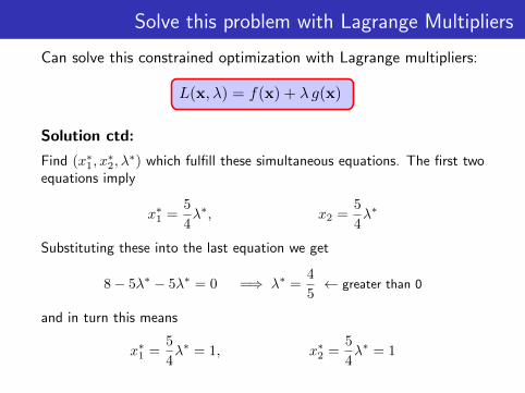
Solve this problem with Lagrange Multipliers
Can solve this constrained optimization with Lagrange multipliers:
L(x, λ) = f(x) + λ g(x)
Solution ctd:
Find (x∗1, x∗2, λ∗) which fulfill these simultaneous equations. The first two
equations imply
x∗1 =5
4λ∗, x2 =
5
4λ∗
Substituting these into the last equation we get
8− 5λ∗ − 5λ∗ = 0 =⇒ λ∗ =4
5← greater than 0
and in turn this means
x∗1 =5
4λ∗ = 1, x∗2 =
5
4λ∗ = 1
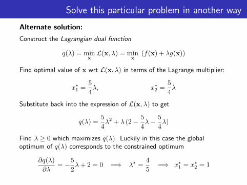
Solve this particular problem in another way
Alternate solution:
Construct the Lagrangian dual function
q(λ) = minxL(x, λ) = min
x(f(x) + λg(x))
Find optimal value of x wrt L(x, λ) in terms of the Lagrange multiplier:
x∗1 =5
4λ, x∗2 =
5
4λ
Substitute back into the expression of L(x, λ) to get
q(λ) =5
4λ2 + λ (2− 5
4λ− 5
4λ)
Find λ ≥ 0 which maximizes q(λ). Luckily in this case the globaloptimum of q(λ) corresponds to the constrained optimum
∂q(λ)
∂λ= −5
2λ+ 2 = 0 =⇒ λ∗ =
4
5=⇒ x∗1 = x∗2 = 1
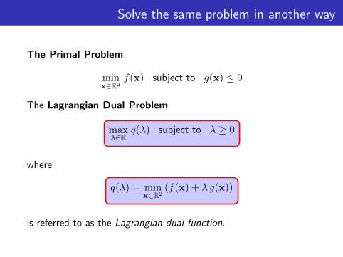
Solve the same problem in another way
The Primal Problem
minx∈R2
f(x) subject to g(x) ≤ 0
The Lagrangian Dual Problem
maxλ∈R
q(λ) subject to λ ≥ 0
where
q(λ) = minx∈R2
(f(x) + λ g(x))
is referred to as the Lagrangian dual function.
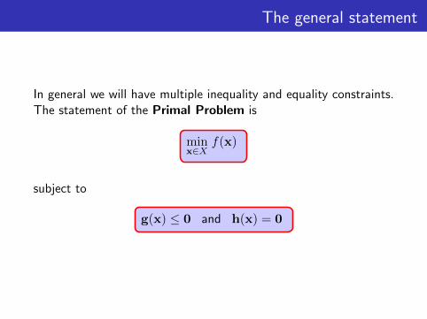
The general statement
In general we will have multiple inequality and equality constraints.The statement of the Primal Problem is
minx∈X
f(x)
subject to
g(x) ≤ 0 and h(x) = 0
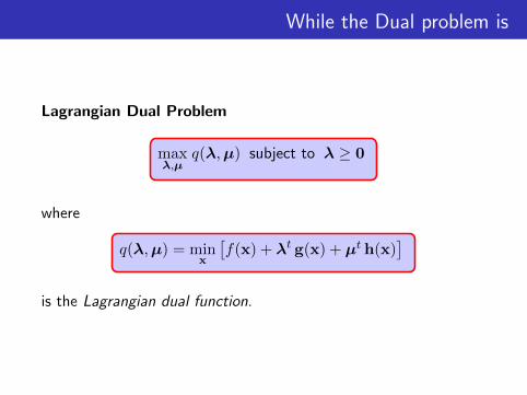
While the Dual problem is
Lagrangian Dual Problem
maxλ,µ
q(λ,µ) subject to λ ≥ 0
where
q(λ,µ) = minx
[f(x) + λt g(x) + µt h(x)
]is the Lagrangian dual function.
Why ??
This dual approach is not guaranteed to succeed. However,
• It does for a certain class of functions
• In these cases it often leads to a simpler optimization problem.
• Particularly in the case when the dimension of x is muchlarger than the number of constraints.
• The expression of x∗ in terms of the Lagrange multipliers maygive some insight into the optimal solution i.e. the optimalseparating hyper-plane found by the SVM.
We will now focus on the geometry of the dual solution...
Geometry of the Dual Problem
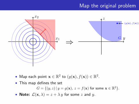
Map the original problem
x1
x2
⇒ y
z(g(x), f(x))
G
• Map each point x ∈ R2 to (g(x), f(x)) ∈ R2.
• This map defines the setG = {(y, z) | y = g(x), z = f(x) for some x ∈ R2}.
• Note: L(x, λ) = z + λ y for some z and y.
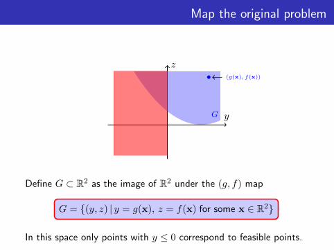
Map the original problem
y
z(g(x), f(x))
G
Define G ⊂ R2 as the image of R2 under the (g, f) map
G = {(y, z) | y = g(x), z = f(x) for some x ∈ R2}
In this space only points with y ≤ 0 correspond to feasible points.
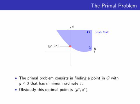
The Primal Problem
y
z(g(x), f(x))
G(y∗, z∗)
• The primal problem consists in finding a point in G withy ≤ 0 that has minimum ordinate z.
• Obviously this optimal point is (y∗, z∗).
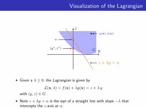
Visualization of the Lagrangian
y
z(g(x), f(x))
G(y∗, z∗)
α
z + λy = α
• Given a λ ≥ 0, the Lagrangian is given by
L(x, λ) = f(x) + λg(x) = z + λ y
with (y, z) ∈ G.
• Note z + λy = α is the eqn of a straight line with slope −λ thatintercepts the z-axis at α.
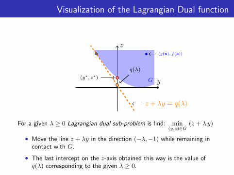
Visualization of the Lagrangian Dual function
y
z(g(x), f(x))
G(y∗, z∗)
q(λ)
z + λy = q(λ)
For a given λ ≥ 0 Lagrangian dual sub-problem is find: min(y,z)∈G
(z + λ y)
• Move the line z + λy in the direction (−λ,−1) while remaining incontact with G.
• The last intercept on the z-axis obtained this way is the value ofq(λ) corresponding to the given λ ≥ 0.
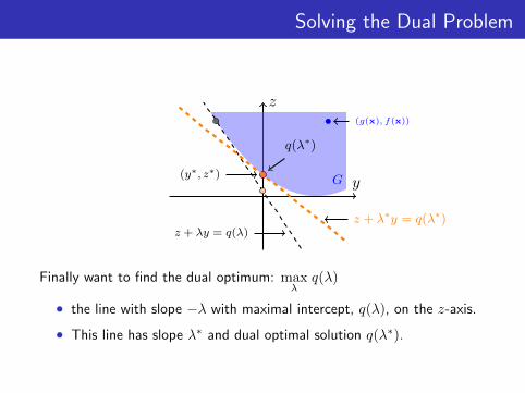
Solving the Dual Problem
y
z(g(x), f(x))
G(y∗, z∗)
z + λy = q(λ)z + λ∗y = q(λ∗)
q(λ∗)
Finally want to find the dual optimum: maxλ
q(λ)
• the line with slope −λ with maximal intercept, q(λ), on the z-axis.
• This line has slope λ∗ and dual optimal solution q(λ∗).
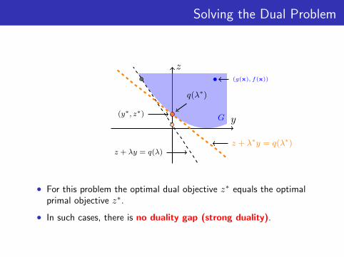
Solving the Dual Problem
y
z(g(x), f(x))
G(y∗, z∗)
z + λy = q(λ)z + λ∗y = q(λ∗)
q(λ∗)
• For this problem the optimal dual objective z∗ equals the optimalprimal objective z∗.
• In such cases, there is no duality gap (strong duality).
Properties of the Lagrangian Dual Function
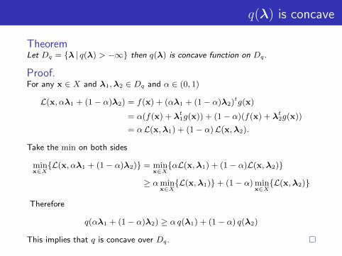
q(λ) is concave
TheoremLet Dq = {λ | q(λ) > −∞} then q(λ) is concave function on Dq.
Proof.For any x ∈ X and λ1,λ2 ∈ Dq and α ∈ (0, 1)
L(x, αλ1 + (1− α)λ2) = f(x) + (αλ1 + (1− α)λ2)tg(x)
= α(f(x) + λt1g(x)) + (1− α)(f(x) + λt
2g(x))
= αL(x,λ1) + (1− α)L(x,λ2).
Take the min on both sides
minx∈X{L(x, αλ1 + (1− α)λ2)} = min
x∈X{αL(x,λ1) + (1− α)L(x,λ2)}
≥ αminx∈X{L(x,λ1)}+ (1− α) min
x∈X{L(x,λ2)}
Therefore
q(αλ1 + (1− α)λ2) ≥ α q(λ1) + (1− α) q(λ2)
This implies that q is concave over Dq.
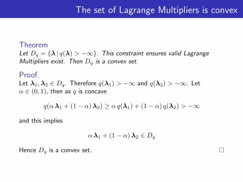
The set of Lagrange Multipliers is convex
TheoremLet Dq = {λ | q(λ) > −∞}. This constraint ensures valid LagrangeMultipliers exist. Then Dq is a convex set.
Proof.Let λ1,λ2 ∈ Dq. Therefore q(λ1) > −∞ and q(λ2) > −∞. Letα ∈ (0, 1), then as q is concave
q(αλ1 + (1− α)λ2) ≥ α q(λ1) + (1− α) q(λ2) > −∞
and this implies
αλ1 + (1− α)λ2 ∈ Dq
Hence Dq is a convex set.
Significance of these results
• The dual is always concave, irrespective of the primal problem.
• Therefore finding the optimum of the dual function is aconvex optimization problem.

Weak Duality
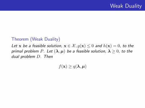
Weak Duality
Theorem (Weak Duality)
Let x be a feasible solution, x ∈ X , g(x) ≤ 0 and h(x) = 0, to theprimal problem P . Let (λ,µ) be a feasible solution, λ ≥ 0, to thedual problem D. Then
f(x) ≥ q(λ,µ)
Weak Duality
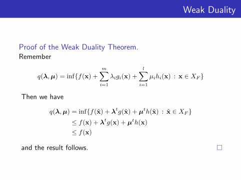
Proof of the Weak Duality Theorem.Remember
q(λ,µ) = inf{f(x) +m∑i=1
λigi(x) +
l∑i=1
µihi(x) : x ∈ XF }
Then we have
q(λ,µ) = inf{f(x̃) + λtg(x̃) + µth(x̃) : x̃ ∈ XF }≤ f(x) + λtg(x) + µth(x)
≤ f(x)
and the result follows.
Weak Duality
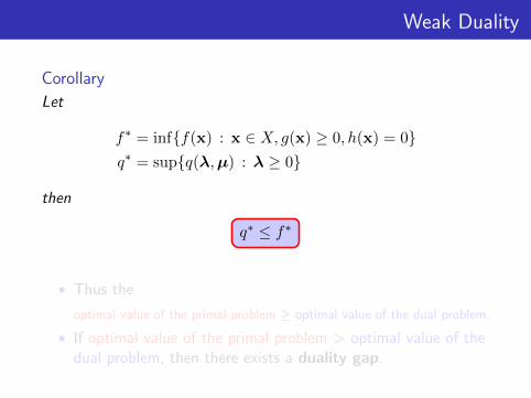
Corollary
Let
f∗ = inf{f(x) : x ∈ X, g(x) ≥ 0, h(x) = 0}q∗ = sup{q(λ,µ) : λ ≥ 0}
then
q∗ ≤ f∗
• Thus the
optimal value of the primal problem ≥ optimal value of the dual problem.
• If optimal value of the primal problem > optimal value of thedual problem, then there exists a duality gap.
Weak Duality
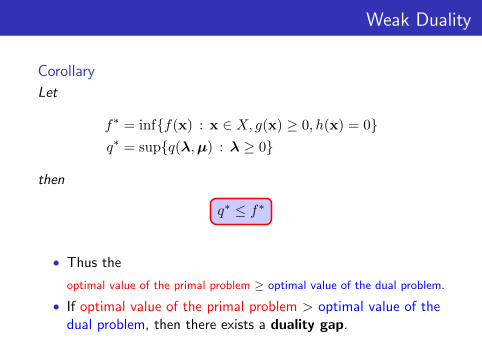
Corollary
Let
f∗ = inf{f(x) : x ∈ X, g(x) ≥ 0, h(x) = 0}q∗ = sup{q(λ,µ) : λ ≥ 0}
then
q∗ ≤ f∗
• Thus the
optimal value of the primal problem ≥ optimal value of the dual problem.
• If optimal value of the primal problem > optimal value of thedual problem, then there exists a duality gap.
Example with a Duality Gap
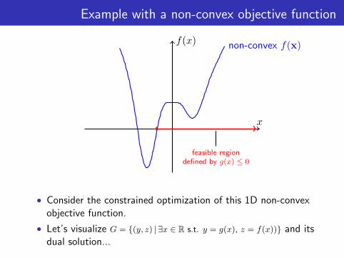
Example with a non-convex objective function
x
f(x) non-convex f(x)
feasible regiondefined by g(x) ≤ 0
• Consider the constrained optimization of this 1D non-convexobjective function.
• Let’s visualize G = {(y, z) | ∃x ∈ R s.t. y = g(x), z = f(x))} and itsdual solution...
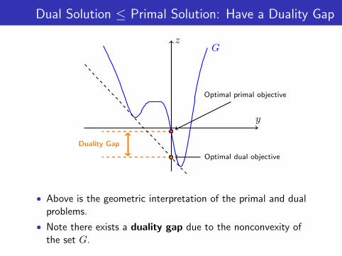
Dual Solution ≤ Primal Solution: Have a Duality Gap
y
z
Duality Gap
G
Optimal primal objective
Optimal dual objective
• Above is the geometric interpretation of the primal and dualproblems.
• Note there exists a duality gap due to the nonconvexity ofthe set G.

Strong Duality
When does Dual Solution = Primal Solution?
The Strong Duality Theorem states, that if some suitableconvexity conditions are satisfied, then there is no duality gapbetween the primal and dual optimisation problems.
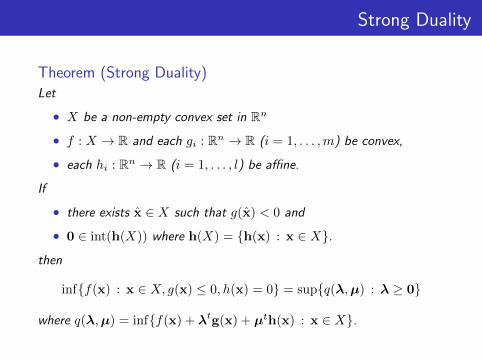
Strong Duality
Theorem (Strong Duality)Let
• X be a non-empty convex set in Rn
• f : X → R and each gi : Rn → R (i = 1, . . . ,m) be convex,
• each hi : Rn → R (i = 1, . . . , l) be affine.
If
• there exists x̂ ∈ X such that g(x̂) < 0 and
• 0 ∈ int(h(X)) where h(X) = {h(x) : x ∈ X}.
then
inf{f(x) : x ∈ X, g(x) ≤ 0, h(x) = 0} = sup{q(λ,µ) : λ ≥ 0}
where q(λ,µ) = inf{f(x) + λtg(x) + µth(x) : x ∈ X}.
Strong Duality
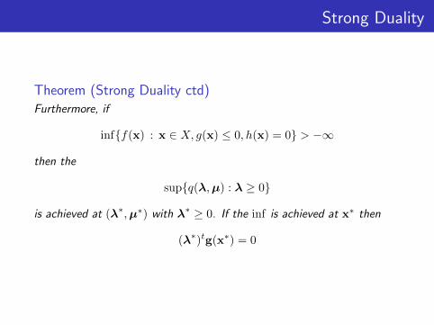
Theorem (Strong Duality ctd)Furthermore, if
inf{f(x) : x ∈ X, g(x) ≤ 0, h(x) = 0} > −∞
then the
sup{q(λ,µ) : λ ≥ 0}
is achieved at (λ∗,µ∗) with λ∗ ≥ 0. If the inf is achieved at x∗ then
(λ∗)tg(x∗) = 0