Kernel–Based Meshless...

Kernel–Based Meshless Methods

R. Schaback

July 18, 2007

Contents

1 Introduction 1

2 Kernels 12.1 Basics . . . . . . . . . . . . . . . . . . . . . . . . . . . . . . . . . . . . . . . . . 12.2 Positive Definiteness . . . . . . . . . . . . . . . . . . . . . . . . . . . . . . . . . 42.3 General Rules . . . . . . . . . . . . . . . . . . . . . . . . . . . . . . . . . . . . 52.4 Inner Product . . . . . . . . . . . . . . . . . . . . . . . . . . . . . . . . . . . . . 72.5 Duality . . . . . . . . . . . . . . . . . . . . . . . . . . . . . . . . . . . . . . . . . 92.6 Native Space . . . . . . . . . . . . . . . . . . . . . . . . . . . . . . . . . . . . . 102.7 Reproducing Kernel Hilbert Spaces . . . . . . . . . . . . . . . . . . . . . . . . . 122.8 Kernels for Orthogonal Expansions . . . . . . . . . . . . . . . . . . . . . . . . . 132.9 Native Spaces of Mercer Kernels . . . . . . . . . . . . . . . . . . . . . . . . . . . 172.10 Finite Case . . . . . . . . . . . . . . . . . . . . . . . . . . . . . . . . . . . . . . 192.11 Kernels for Univariate Sobolev Spaces . . . . . . . . . . . . . . . . . . . . . . . . 20

3 Optimal Recovery 243.1 Optimality Properties . . . . . . . . . . . . . . . . . . . . . . . . . . . . . . . . . 243.2 Lagrange Reformulation . . . . . . . . . . . . . . . . . . . . . . . . . . . . . . . 263.3 Calculation . . . . . . . . . . . . . . . . . . . . . . . . . . . . . . . . . . . . . . 293.4 Regularization . . . . . . . . . . . . . . . . . . . . . . . . . . . . . . . . . . . . . 30

4 Conditionally Positive Definite Kernels 344.1 Splines . . . . . . . . . . . . . . . . . . . . . . . . . . . . . . . . . . . . . . . . . 354.2 General Case . . . . . . . . . . . . . . . . . . . . . . . . . . . . . . . . . . . . . 434.3 Inner Products . . . . . . . . . . . . . . . . . . . . . . . . . . . . . . . . . . . . 464.4 Optimal Recovery . . . . . . . . . . . . . . . . . . . . . . . . . . . . . . . . . . . 474.5 Projector to IP . . . . . . . . . . . . . . . . . . . . . . . . . . . . . . . . . . . . 504.6 Native Space . . . . . . . . . . . . . . . . . . . . . . . . . . . . . . . . . . . . . 53

5 Practical Observations 565.1 Lagrange Interpolation . . . . . . . . . . . . . . . . . . . . . . . . . . . . . . . . 575.2 Interpolation of Mixed Data . . . . . . . . . . . . . . . . . . . . . . . . . . . . . 585.3 Error Behavior . . . . . . . . . . . . . . . . . . . . . . . . . . . . . . . . . . . . 595.4 Stability . . . . . . . . . . . . . . . . . . . . . . . . . . . . . . . . . . . . . . . . 60

i

5.5 Uncertainty Principle . . . . . . . . . . . . . . . . . . . . . . . . . . . . . . . . . 615.6 Scaling . . . . . . . . . . . . . . . . . . . . . . . . . . . . . . . . . . . . . . . . . 625.7 Practical Rules . . . . . . . . . . . . . . . . . . . . . . . . . . . . . . . . . . . . 645.8 Sensitivity to Noise . . . . . . . . . . . . . . . . . . . . . . . . . . . . . . . . . . 66

6 Error Analysis 696.1 Sampling Inequalities . . . . . . . . . . . . . . . . . . . . . . . . . . . . . . . . . 696.2 Univariate Case . . . . . . . . . . . . . . . . . . . . . . . . . . . . . . . . . . . . 716.3 Example: Univariate Splines . . . . . . . . . . . . . . . . . . . . . . . . . . . . 726.4 Univariate Polynomial Reproduction . . . . . . . . . . . . . . . . . . . . . . . . 736.5 Norming Sets . . . . . . . . . . . . . . . . . . . . . . . . . . . . . . . . . . . . . 766.6 Multivariate Polynomial Reproduction . . . . . . . . . . . . . . . . . . . . . . . 766.7 Moving Least Squares . . . . . . . . . . . . . . . . . . . . . . . . . . . . . . . . 816.8 Bramble–Hilbert Lemma . . . . . . . . . . . . . . . . . . . . . . . . . . . . . . . 846.9 Globalization . . . . . . . . . . . . . . . . . . . . . . . . . . . . . . . . . . . . . 876.10 Error Bounds . . . . . . . . . . . . . . . . . . . . . . . . . . . . . . . . . . . . . 88

7 Construction of Kernels 897.1 General Construction Techniques . . . . . . . . . . . . . . . . . . . . . . . . . . 897.2 Special Kernels on IRd . . . . . . . . . . . . . . . . . . . . . . . . . . . . . . . . 907.3 Translation–Invariant Kernels on IRd . . . . . . . . . . . . . . . . . . . . . . . . 917.4 Global Sobolev Kernels on IRd . . . . . . . . . . . . . . . . . . . . . . . . . . . . 947.5 Native Spaces of Translation–Invariant Kernels . . . . . . . . . . . . . . . . . . . 957.6 Construction of Positive Definite Radial Functions on IRd . . . . . . . . . . . . . 977.7 Conditionally Positive Definite Kernels . . . . . . . . . . . . . . . . . . . . . . . 1107.8 Examples . . . . . . . . . . . . . . . . . . . . . . . . . . . . . . . . . . . . . . . 1117.9 Connection to L2(IR

d) . . . . . . . . . . . . . . . . . . . . . . . . . . . . . . . . 1127.10 Characterization of Native Spaces . . . . . . . . . . . . . . . . . . . . . . . . . . 1157.11 Connection to Sobolev Spaces . . . . . . . . . . . . . . . . . . . . . . . . . . . . 116

8 Stability Theory 1178.1 Uncertainty Relation . . . . . . . . . . . . . . . . . . . . . . . . . . . . . . . . . 1178.2 Lower Bounds on Eigenvalues . . . . . . . . . . . . . . . . . . . . . . . . . . . . 1198.3 Stability in Function Space . . . . . . . . . . . . . . . . . . . . . . . . . . . . . . 123

9 Hilbert Space Theory 1279.1 Normed Linear Spaces . . . . . . . . . . . . . . . . . . . . . . . . . . . . . . . . 1289.2 Pre–Hilbert Spaces . . . . . . . . . . . . . . . . . . . . . . . . . . . . . . . . . . 1299.3 Sequence Spaces . . . . . . . . . . . . . . . . . . . . . . . . . . . . . . . . . . . . 1309.4 Best Approximations . . . . . . . . . . . . . . . . . . . . . . . . . . . . . . . . . 1309.5 Hilbert Spaces . . . . . . . . . . . . . . . . . . . . . . . . . . . . . . . . . . . . . 1329.6 Riesz Representation Theorem . . . . . . . . . . . . . . . . . . . . . . . . . . . . 1349.7 Reproducing Kernel Hilbert Spaces . . . . . . . . . . . . . . . . . . . . . . . . . 1369.8 Completion of Pre–Hilbert Spaces . . . . . . . . . . . . . . . . . . . . . . . . . . 1369.9 Applications . . . . . . . . . . . . . . . . . . . . . . . . . . . . . . . . . . . . . . 139

ii

10 Necessary Results from Real Analysis 14010.1 Lebesgue Integration . . . . . . . . . . . . . . . . . . . . . . . . . . . . . . . . . 14010.2 Fourier Transforms on IRd . . . . . . . . . . . . . . . . . . . . . . . . . . . . . . 14210.3 Fourier Transform in L2(IR

d) . . . . . . . . . . . . . . . . . . . . . . . . . . . . 14610.4 Poisson Summation Formula . . . . . . . . . . . . . . . . . . . . . . . . . . . . . 14610.5 Fourier Transforms of Functionals . . . . . . . . . . . . . . . . . . . . . . . . . . 14810.6 Special Functions and Transforms . . . . . . . . . . . . . . . . . . . . . . . . . . 150

iii

1 Introduction

This is a text intended for use with my lecture “Approximationsverfahren II” in summer 2007.Though the basic background material is in the book [71] of Holger Wendland, some additionalstuff is necessary at certain places, and I recycled larger parts of a 1997 lecture handout.

The text is under construction at various marked places, and it will evolve during the summerterm. The chapter numbering is aligned with the numbering in the actual lecture and with theaccompanying slides.

Gottingen, July 18, 2007

R. Schaback

2 Kernels

This chapter contains a collection of results on positive semidefinite kernels, while the majorliterature focuses on positive definite kernels. See the old book of Meschkowski [42] and therecent dissertation of Roland Opfer [52].

2.1 Basics

Definition 2.1 Let Ω be an arbitrary nonempty set. A function

K : Ω × Ω → IR or C

is called a (real– or complex–valued) kernel on Ω. We call K a hermitian kernel if

K(x, y) = K(y, x) for all x, y ∈ Ω.

If the kernel is real–valued, this property defines a symmetric kernel.

In most cases, we shall use only real–valued symmetric kernels, but for certain argumentswe shall have to allow complex–valued kernels. For practical applications, one can considerhermitian kernels only, because for any kernel K we can go over to the hermitian kernel

K(x, y) :=1

2(K(x, y) +K(y, x)) for all x, y ∈ Ω.

To Do: convert everything as far as possible to allow complex–valued kernels.

Remember that Ω does not carry any structure at all. It can contain texts and images, forinstance, and it will often be infinite. Some readers may consider this as being far too general.However, in the context of learning algorithms, the set Ω defines the possible learning inputs.Thus Ω should be general enough to allow Shakespeare texts or X-ray images, i.e. Ω shouldbetter have no predefined structure at all. Thus the kernels occurring in machine learning [65]are extremely general, but still they take a special form which can be tailored to meet thedemands of applications. We shall later explain the recipes for their definition and usage.

1

In certain situations, a kernel is given a-priori, e.g. the Gaussian

K(x, y) := exp(−‖x− y‖22) for all x, y ∈ Ω := IRd. (2.2)

Each specific choice of a predefined kernel has a number of important and possibly unexpectedconsequences which we shall describe later.

If no predefined kernel is available for a certain set Ω, an application-dependent feature mapΦ : Ω → F with values in a Hilbert “feature” space F is defined. It should provide for eachx ∈ Ω a large collection Φ(x) of features of x which are characteristic for x and which livein the Hilbert space F of high or even infinite dimension. Note the F has plenty of usefulstructure, while Ω has not. Feature maps Ω → F allow to apply linear techniques in theirrange F , while their domain Ω is an unstructured set. They should be chosen carefully in anapplication-dependent way, capturing the essentials of elements of Ω.

With a feature map Φ at hand, there is a kernel

K(x, y) := (Φ(x),Φ(y))F for all x, y ∈ Ω (2.3)

which is automatically hermitian.

In another important class of cases, the set Ω consists of random variables. Then the covariancebetween two random variables x and y from Ω is a standard choice of a kernel. These and otherkernels arising in nondeterministic settings are dealt with in books on statistics. The connectionto learning is obvious: two learning inputs x and y from Ω should be very similar, if they areclosely “correlated”, if they have very similar features, or if (2.3) takes large positive values.These examples again suggest to focus on symmetric kernels.

A kernel K on Ω defines a function K(·, y) for all fixed y ∈ Ω. This allows to generate andmanipulate spaces

K0 := span K(·, y) : y ∈ Ω. (2.4)

of functions on Ω. In Learning Theory, the function K(·, y) = (Φ(·),Φ(y))F relates each otherinput object to a fixed object y via its essential features. But in general K0 just provides ahandy linear space of trial functions on Ω which is extremely useful for most applications ofkernels, e.g. when Ω consists of texts or images. For example, in meshless methods for solvingpartial differential equations, certain finite-dimensional subspaces of K0 are used as trial spacesto furnish good approximations to the solutions.

In certain other cases, the set Ω carries a measure µ, and then, under reasonable assumptionslike f, K(y, ·) ∈ L2(Ω, µ), the generalized convolution

K ∗Ω f :=∫

Ωf(x)K(·, x)dµ(x) (2.5)

defines an integral transform f 7→ K ∗Ω f which can be very useful. Note that Fourier orHankel transforms arise this way, and recall the role of the Dirichlet kernel in Fourier analysisof univariate periodic functions. The above approach to kernels via convolution works on locallycompact topological groups using Haar measure, but we do not want to pursue this detour intoabstract harmonic analysis too far. For space reasons, we also have to exclude complex-valuedkernels and all transform-type applications of kernels here, but it should be pointed out that

2

wavelets are special kernels of the above form, defining the continuous wavelet transform thisway.

Note that discretization of the integral in the convolution transform leads to functions in thespace K0 from (2.4). Using kernels as trial functions can be viewed as a discretized convolution.This is a very useful fact in the theoretical analysis of kernel-based techniques.

At this point, we skip over the various other occurrences of kernels in the mathematical literatureand in applications (see the survey article [63]). Just keep in mind that kernels have three majorapplication fields: they generate convolutions, trial spaces, and covariances. The first two arerelated by discretization.

But we recall that in machine learning and various other cases there are kernels of the Hilbert–Schmidt or Mercer form

K(x, y) =∑

i∈I

λiϕi(x)ϕi(y) for all x, y ∈ Ω (2.6)

with certain functions ϕ : Ω → IR, i ∈ I, certain positive weights λi, i ∈ I and an indexset I such that the summability conditions

K(x, x) :=∑

i∈I

λiϕ2i (x) <∞ (2.7)

hold for all x ∈ Ω. Note that this occurs in machine learning, if the functions ϕi each describea feature of x, and if the feature space is the weighted ℓ2 space

ℓ2,I,λ := ξii∈I :∑

i∈I

λiξ2i <∞ (2.8)

of sequences with indices in I. But it also occurs when kernels generating positive integraloperators are expanded into eigenfunctions ϕi on Ω (see Mercer’s theorem 2.14 below), andsuch kernels can be viewed as arising from generalized convolution.

Note further that the summability condition (2.7) guarantees the well–definedness of the kernelby the Cauchy–Schwarz inequality

|K(x, y)| =

∣∣∣∣∣∑

i∈I

(√λiϕi(x)

)·(√

λiϕi(y))∣∣∣∣∣ ≤

√K(x, x)K(y, y) for all x, y ∈ Ω.

But there are many other kernels that have the above form. For instance, the univariateGaussian kernel is

K(x, y) := exp(−(x− y)2)= exp(−x2) exp(2xy) exp(−y2)

= exp(−x2)

( ∞∑

n=0

2n

n!xnyn

)exp(−y2)

=∞∑

n=0

2n

n!xn exp(−x2)︸︷︷︸

=:ϕn(x)

yn exp(−y2)︸︷︷︸

=:ϕn(y)

=∞∑

n=0

2n

n!ϕn(x)ϕn(y) for all x, y ∈ IR

without summability problems. But we shall postpone the construction of large classes ofkernels to a later chapter.

3

2.2 Positive Definiteness

If we have an arbitrary set X = x1, . . . , xN of N distinct elements of Ω and a symmetrickernel K on Ω, we can form linear combinations

s(x) :=N∑

j=1

ajK(xj , x), x ∈ Ω (2.9)

of “translates” of the kernel. This is a very convenient technique to generate functions on anotherwise unstructured set Ω.

With such a set X = x1, . . . , xN we can form the symmetric N ×N kernel matrix

A := AK,X,X := (K(xj , xk))1≤j,k≤N (2.10)

and pose the interpolation problem

yk = s(xk), 1 ≤ k ≤ N

yk =N∑

j=1

ajK(xj , xk), 1 ≤ k ≤ N.(2.11)

In matrix notation, this is an N ×N linear system

AK,X,Xa = y.

In general, solvability of such a system is a serious problem, but one of the central features ofkernels and radial basis functions is to make this problem obsolete via

Definition 2.12 A kernel K on Ω is called positive (semi–) definite, if for all sets X =x1, . . . , xN of N distinct elements of Ω and all N the N×N kernel matrix (2.10) is positive(semi–) definite. This means in the complex–valued case that the quadratic form

a ∈ Cn 7→N∑

j,k=1

ajakK(xj , xk)

is nonnegative, while in the positive definite case it is zero only if the vector a is zero.

Theorem 2.13 Hilbert–Schmidt or Mercer kernels of the form (2.6) are positive semidefinite.Also, kernels arising from feature maps via (2.3) are positive semidefinite.

Proof: The second statement is obvious, because kernels from feature maps generate kernelmatrices that are Gramian matrices, and these are always positive semidefinite. To prove thefirst part, the quadratic form corresponding to the kernel matrix can be written as

aTAK,X,Xa =N∑

j,k=1

ajakK(xj , xk)

=N∑

j,k=1

ajak

∑

i∈I

λiϕi(xj)ϕi(xk)

=∑

i∈I

λi

N∑

j=1

ajϕi(xj)N∑

k=1

akϕi(xk)

=∑

i∈I

λi

N∑

j=1

ajϕi(xj)

2

≥ 0

4

for all vectors a ∈ IRN . 2

At this point, we stick to positive semidefiniteness, but later we shall turn to positive definitekernels.

The basic connection of positive semidefinite kernels to a representation (2.6) is Mercer’s

Theorem 2.14 Suppose K is a continuous symmetric positive semidefinite kernel on a closedbounded interval Ω := [a, b] ⊂ IR. Then there is an orthonormal basis ϕii∈IN of L2[a, b] con-sisting of eigenfunctions of the linear integral operator defined by K such that the correspondingsequence of eigenvalues λi is nonnegative. This means

∫ b

aK(x, y)ϕi(y)dy = λiϕi(x) for all x ∈ [a, b], i ∈ IN.

The eigenfunctions corresponding to non-zero eigenvalues are continuous on [a, b] and K hasthe representation (2.6), where the convergence is absolute and uniform.

This theorem is contained in all reasonable books on Integral Equations or Functional Analysis.The background fact is that the operator

ϕ 7→∫ b

aK(x, y)ϕ(y)dy

is a compact “positive ” integral operator on L2[a, b], and Mercer’s theorem is a consequenceof standard spectral theory in Hilbert spaces. Furthermore, all of this generalizes to domainsand kernels in more than one dimension.

2.3 General Rules

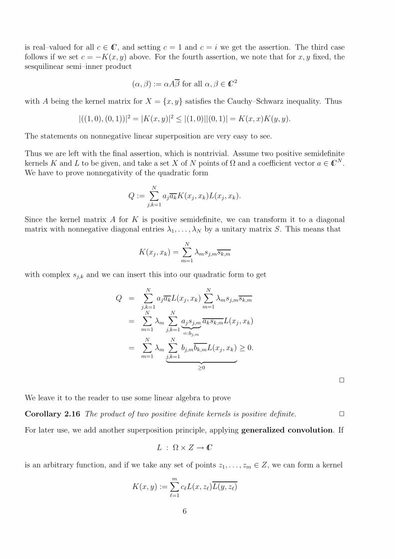
We state some useful results on positive (semi)–definite kernels on some domain Ω.

Theorem 2.15 Let K be a positive semidefinite kernel on Ω. Then

K(x, x) ≥ 0 for all x ∈ Ω,

K(y, x) = K(x, y) for all x, y ∈ Ω,2|K(x, y)|2 ≤ K(x, x) +K(y, y) for all x, y ∈ Ω,|K(x, y)|2 ≤ K(x, x) ·K(y, y) for all x, y ∈ Ω.

Furthermore, any finite linear combination of positive semidefinite kernels with nonnegativecoefficients yields a positive definite kernel (this means that positive definite kernels form aconvex cone). If one of the kernels is positive definite, and if its factor is positive, thesuperposition of kernels is positive definite. Finally, the product of two positive semidefinitekernels is positive semidefinite.

Proof: For the first property, use X = x in Definition 2.12. The second property impliesthat positive semidefinite kernels are always hermitian, and the proof uses X = x, y andcoefficients (1, c) with c ∈ C . Then

K(x, x) +K(y, y) + cK(x, y) + cK(y, x) ≥ 0

5

is real–valued for all c ∈ C , and setting c = 1 and c = i we get the assertion. The third casefollows if we set c = −K(x, y) above. For the fourth assertion, we note that for x, y fixed, thesesquilinear semi–inner product

(α, β) := αAβ for all α, β ∈ C 2

with A being the kernel matrix for X = x, y satisfies the Cauchy–Schwarz inequality. Thus

|((1, 0), (0, 1))|2 = |K(x, y)|2 ≤ |(1, 0)||(0, 1)| = K(x, x)K(y, y).

The statements on nonnegative linear superposition are very easy to see.

Thus we are left with the final assertion, which is nontrivial. Assume two positive semidefinitekernels K and L to be given, and take a set X of N points of Ω and a coefficient vector a ∈ CN .We have to prove nonnegativity of the quadratic form

Q :=N∑

j,k=1

ajakK(xj , xk)L(xj , xk).

Since the kernel matrix A for K is positive semidefinite, we can transform it to a diagonalmatrix with nonnegative diagonal entries λ1, . . . , λN by a unitary matrix S. This means that

K(xj , xk) =N∑

m=1

λmsj,msk,m

with complex sj,k and we can insert this into our quadratic form to get

Q =N∑

j,k=1

ajakL(xj , xk)N∑

m=1

λmsj,msk,m

=N∑

m=1

λm

N∑

j,k=1

ajsj,m︸︷︷︸=:bj,m

aksk,mL(xj , xk)

=N∑

m=1

λm

N∑

j,k=1

bj,mbk,mL(xj , xk)

︸︷︷︸≥0

≥ 0.

2

We leave it to the reader to use some linear algebra to prove

Corollary 2.16 The product of two positive definite kernels is positive definite. 2

For later use, we add another superposition principle, applying generalized convolution. If

L : Ω × Z → C

is an arbitrary function, and if we take any set of points z1, . . . , zm ∈ Z, we can form a kernel

K(x, y) :=m∑

ℓ=1

cℓL(x, zℓ)L(y, zℓ)

6

when taking nonnegative coefficients c1, . . . , cm. The kernel K will be hermitian, and positivesemidefinite due to

N∑

j,k=1

ajakK(xj , xk)

=N∑

j,k=1

ajak

m∑

ℓ=1

cℓL(xj , zℓ)L(xk, zℓ)

=m∑

ℓ=1

cℓN∑

j,k=1

ajL(xj , zℓ)akL(xk, zℓ)

=m∑

ℓ=1

cℓ

∣∣∣∣∣∣

N∑

j=1

ajL(xj , zℓ)

∣∣∣∣∣∣

2

≥ 0.

This generalizes easily to cases where the sum can be replaced by an integral, e.g.

K(x, y) :=∫

Zc(z)L(x, z)L(y, z)dz, x, y ∈ Ω

with a nonnegative function c, provided that the above is well–defined and finite. This holdswhenever

K(x, x) =∫

Zc(z)|L(x, z)|2dz

is well–defined and finite for all x ∈ Ω, due to the Cauchy–Schwarz inequality. Applyingmeasure theory, on can also go over to

K(x, y) :=∫

ZL(x, z)L(y, z)dµ(z), x, y ∈ Ω

with a nonnegative measure µ on Z, using

K(x, x) =∫

Z|L(x, z)|2dµ(z)

as a sufficient condition for well–definedness of the new kernel.

But note that the above argument is nothing else than the transition to a suitable feature space.If

Φ(x) := L(x, ·)maps Ω into a suitable function space F consisting of functions on Z as a feature space, we canwrite each instance of the above construction in the form (2.3). Thus positive semidefinitenessof such kernels is no miracle.

2.4 Inner Product

The following construction is of utmost importance for kernel–based techniques. We assume Kto be a symmetric real–valued positive semidefinite kernel on Ω, and we form the space

S := SΩ := span K(x, ·) : x ∈ Ω (2.17)

of all finite linear combinations of the functions K(x, ·) : Ω → IR. Note that general elementsfrom S take the form

fa,X(·) =N∑

j=1

ajK(xj , ·) (2.18)

7

with a ∈ IRN while X = x1, . . . , xN ⊂ Ω, but different N and all point sets X are allowed.

To Do: Convert to complex case...

On S we can define a bilinear form

M∑

j=1

ajK(xj , ·)︸︷︷︸

=:fa,X(·)

,N∑

k=1

bkK(yk, ·)︸︷︷︸

=:fb,Y (·)

K

:=M∑

j=1

N∑

k=1

ajbkK(xj , yk)

=M∑

j=1

ajfb,Y (xj)

=N∑

k=1

bkfa,X(yk).

(2.19)

To prove that it is well–defined, we re–represent the functions fa,X and fb,Y in different form as

fa,X =M∑

j=1

ajK(xj , ·) = fa,X

fb,Y =N∑

k=1

bkK(yk, ·) = fb,Y

and check the result:

(fa,X , fb,Y )K =M∑

j=1

N∑

k=1

ajbkK(xj , yk)

=M∑

j=1

ajfb,Y (xj)

=M∑

j=1

aj

N∑

k=1

bkK(yk, xj)

=N∑

k=1

bkM∑

j=1

ajK(yk, xj)

=N∑

k=1

bkfa,X(yk)

=N∑

k=1

bkM∑

j=1

ajK(xj , yk)

=M∑

j=1

N∑

k=1

aj bkK(xj , yk)

= (fa,X , fb,Y )K

to see that it is independent of the representation. Furthermore, we have a positive semidefinitebilinear form due to the positive semidefiniteness of all kernel matrices.

When specializing (2.19) partially to functions K(y, ·) based on single points, we get theextremely useful reproduction equation

(f,K(y, ·))K = f(y) for all y ∈ Ω, f ∈ S (2.20)

8

and its special case

(K(x, ·), K(y, ·))K = K(x, y) for all x, y ∈ Ω. (2.21)

Strangely enough, the bilinear form is even positive definite:

Theorem 2.22 If K is a positive semidefinite symmetric kernel on Ω, the bilinear form (., .)K

of (2.19) is positive definite on the space S of (2.17) as a space of functions on Ω. Thus S isa pre–Hilbert or Euclidean space of functions on Ω.

Proof: Assume that

(fa,X , fa,X)K =N∑

j,k=1

ajakK(xj , xk) =N∑

j=1

ajfa,X(xj) = 0

for a ∈ IRN and X = x1, . . . , xN ⊂ Ω. Then by (2.20) and the Cauchy–Schwarz inequalitywe have

|fa,X(x)|2 = |(fa,X , K(x, ·))K |2 ≤ (fa,X , fa,X)K(K(x, ·), K(x, ·))K = 0

for all x ∈ Ω. 2

Note that the above argument does not imply a = 0 for fa,X(·) = 0. But there are some otheruseful implications:

|f(x)| ≤ ‖f‖K

√K(x, x) for all x ∈ Ω, f ∈ S

|f(x) − f(y)| ≤ ‖f‖K

√K(x, x) − 2K(x, y) +K(y, y) for all x, y ∈ Ω, f ∈ S

where we now can use the norm notation for ‖f‖2K = (f, f)K and all f ∈ S.

2.5 Duality

We now consider the dual space S∗ to S. It contains all bounded linear functionals λ on Sand it has a dual norm

‖λ‖S∗ := supf∈S\0

λ(f)

‖f‖K

for all λ ∈ S∗.

But we assert that we can write the dual norm via an inner product which we can define as

(λ, µ)K := (λxK(x, ·), µyK(y, ·))K for all λ, µ ∈ S

where the notation λxK(x, ·) means that λ acts with respect to the variable x. Clearly, theright–hand side is a well–defined bilinear form, but we postpone to prove its positive definitenessfor a moment. Instead, we want to prove the generalized reproduction equation

λ(f) = (f, λxK(x, ·))K for all f ∈ S, λ ∈ S∗. (2.23)

It suffices to do this on all functions fy := K(y, ·), and we get

(fy, λxK(x, ·))K = (K(y, ·), λxK(x, ·))K = λxK(x, y) = λxK(y, x) = λ(fy).

9

Now if (λ, λ)K = 0, we have λxK(x, ·) = 0 on Ω and λ(f) = 0 for all f ∈ S by the generalizedreproduction equation, leading to λ = 0 and proving definiteness of the dual bilinear form.Furthermore, by the definition of the dual norm and the dual bilinear form we have

‖λ‖S∗ = supf∈S\0

λ(f)

‖f‖K

≤ ‖λxK(x, ·)‖K = ‖λ‖K ,

but we get equality for f = λxK(x, ·) due to

λ(λxK(x, ·))‖λxK(x, ·)‖K

=‖λxK(x, ·)‖2

K

‖λxK(x, ·)‖K

= ‖λxK(x, ·)‖K .

This implies that the dual space S∗ of S is again a pre–Hilbert space under the dual innerproduct above.

By the reproduction equation, the point evaluation functionals

δx : S → IR, f 7→ f(x)

satisfyδx(f) = f(x) = (f,K(x, ·)K for all f ∈ S, x ∈ Ω

and thus are bounded and continuous via

|δx(f)| = |f(x)| = |(f,K(x, ·)K | ≤ ‖f‖K‖K(x, ·)‖K = ‖f‖K

√K(x, x) for all f ∈ S, x ∈ Ω.

The dual S∗ of S thus contains all point evaluation functionals, and we get

(δx, δy)K = (K(x, ·), K(y, ·))K = K(x, y) for all x, y ∈ Ω.

In particular, we shall often use the identity

‖δx − δy‖2K = ‖δx‖2

K − 2(δx, δy)K + ‖δy‖2K = K(x, x) − 2K(x, y) +K(y, y) for all x, y ∈ Ω.

This leads to a notion of a distance on Ω via

dist(x, y) := ‖δx − δy‖K =√K(x, x) − 2K(x, y) +K(y, y) for all x, y ∈ Ω.

In this special distance, all functions in S are “continuous” due to

|f(x) − f(y)| ≤ ‖f‖K‖δx − δy‖K = ‖f‖Kdist(x, y) for all x, y ∈ Ω, f ∈ S.

2.6 Native Space

We now know that S is an inner–product or semi–Hilbert space of functions on Ω under theinner product (., .)K , provided that K is a positive semidefinite symmetric kernel on Ω. Thenwe can invoke a classical argument from Hilbert space theory to go over the closure of S under(., .)K . This is an abstract space defined by equivalence classes of Cauchy sequences in S, butit is a complete space (thus a Hilbert space), and each continuous map from S to a Banachspace Y extends uniquely to the closure.

10

Theorem 2.24 Each symmetric positive semidefinite kernel K on a set Ω is the reproducingkernel of a Hilbert space called the native space NK of the kernel. This Hilbert space is unique,and it is a space of functions on Ω. The kernel K is a reproducing kernel of NK in thesense

(f,K(y, ·))K = f(y) for all y ∈ Ω, f ∈ NK

generalizing (2.20).

Proof: The existence of the native space follows from standard Hilbert space arguments we donot repeat here, see section 9.8. Since (2.20) is an equation with both sides being continuouslydependent on f ∈ S, it carries over to the closure and thus to the native space, proving thereproduction formula above. But then it explains how an abstract element f of the native spacecan be interpreted as a function: just use the left–hand side as a definition of the right–handside.

If K is reproducing in a possibly different Hilbert space T with an analogous reproductionequation, we can use (2.21) and the reproduction equation in T to conclude

K(x, y) = (K(x, ·), K(y, ·))K = (K(x, ·), K(y, ·))T ,

and this proves that the inner products of T and NK coincide on S. Since T is a Hilbert space,it must then contain the closure NK of S as a closed subspace. If T were larger than NK , theremust be a nonzero element f ∈ T which is orthogonal to NK and in particular to S. But then

f(y) = (f,K(y, ·))T = 0 for all y ∈ Ω

is a contradiction. 2

Note that usually the Hilbert space closure of an inner–product space is considerably “larger”than the space itself. This is very much like the transition from rational numbers to realnumbers.

We should have a quick look at point evaluation functionals

δx : NK → IR, f 7→ f(x) for all f ∈ NK

for x ∈ Ω. Note that the dual space N ∗K of the native space is again a Hilbert space with an

inner product and norm, which is isometrically isomorphic to NK itself via the Riesz map

R : N ∗K → NK ,

λ(f) = (f, R(λ))K for all f ∈ NK , λ ∈ N ∗K ,

(λ, µ)K = (R(λ), R(µ))K for all λ, µ ∈ N ∗K ,

where we denote the dual inner product in N ∗K again by (., .)K for simplicity.

The reproduction equation tells us that

δx(f) = (f,K(x, ·))K for all f ∈ NK , x ∈ Ω,

and we immediately see that K(x, ·) is the Riesz representer R(δx) of δx in NK , leading directlyto

(δx, δy)K = (R(δx), R(δy))K = (K(x, ·), K(y, ·))K = K(x, y) for all x, y ∈ Ω

11

and‖δx‖K = ‖K(x, ·)‖K =

√K(x, x) for all x ∈ Ω (2.25)

because the Riesz map is an isometry. Similarly, we have the extended reproduction property

λ(f) = (f, λxK(x, ·))K for all f ∈ NK , λ ∈ N ∗K

telling us that λxK(x, ·) is the Riesz representer of λ.

2.7 Reproducing Kernel Hilbert Spaces

The theoretical background for all of this is

Definition 2.26 A Hilbert space H of functions on a set Ω with inner product (., .)H is calleda reproducing kernel Hilbert space (RKHS), if there is a kernel function K : Ω → IRwith K(x, ·) ∈ H for all x ∈ Ω and the reproduction property

f(x) = (f,K(x, ·))H for all x ∈ Ω, f ∈ H.

This implies(K(y, ·), K(x, ·))H = K(y, x) = K(x, y) for all x, y ∈ Ω,

and it is easy to verify that K is positive semidefinite. In fact, if we take X = x1 . . . , xN ⊂ Ωand a vector a ∈ IRN , we get

N∑

j,k=1

ajakK(xj , xk)

=N∑

j,k=1

ajak(K(xj , ·), K(xk, ·))K

=

N∑

j=1

ajK(xj , ·),N∑

k=1

akK(xk, ·)

K

=

∥∥∥∥∥∥

N∑

j=1

ajK(xj , ·)∥∥∥∥∥∥

2

K

≥ 0

so that the kernel matrix is positive semidefinite.

In the previous section we have proven

Theorem 2.27 Every positive semidefinite symmetric kernel K on some set Ω is the reproduc-ing kernel of some (“native”) Hilbert space NK of functions on Ω in which the point evaluationfunctionals δx are continuous and have the kernel functions K(x, ·) as Riesz representers. 2

Now we go for the converse:

Theorem 2.28 Let H be a Hilbert space of functions on Ω such that all point evaluationfunctionals

δx : f 7→ f(x) for all f ∈ Hfor x ∈ Ω are continuous. Then H is a reproducing kernel Hilbert space with a positive semidef-inite kernel K on Ω, and the kernel is uniquely defined by providing the Riesz representers ofthe point evaluation functionals. Finally, the space H is the native space for the kernel.

12

Proof: Under the hypothesis of the theorem, there must be a Riesz representer of δx, and bydefinition of the Riesz map it takes the form K(x, ·) ∈ H satisfying the reproduction equation.Thus any such Hilbert space has a positive semidefinite symmetric reproducing kernel. Thefinal assertion follows from Theorem 2.24, because both the native space and H are Hilbertspaces which contain all K(x, ·). 2

2.8 Kernels for Orthogonal Expansions

Let us look at the special case where a Hilbert space H has a complete orthonormal basis ϕii∈I

of functions in Ω. A special case are trigonometric polynomials in the space of square–integrable2π–periodic functions, or any space of functions spanned by orthogonal polynomials.

Then each f ∈ H has a unique expansion

f =∑

i∈I

(f, ϕi)Hϕi

with the Parseval equation‖f‖2

H =∑

i∈I

(f, ϕi)2H <∞.

In many cases, including trigonometric or orthogonal algebraic polynomials, the expansions offunctions in H do not converge pointwise, but only in the Hilbert space norm. Thus point–evaluation functionals are not continuous on H. The situation is better if the coefficients of theexpansion satisfies a decay condition, and this condition defines a closed space of H if posedcorrectly. An example for trigonometric series

f(x) =a0

2+

∞∑

n=1

(an cos(nx) + bn sin(nx)) (2.29)

is the condition ∞∑

n=1

n2(a2

n + b2n)<∞

because it implies that the series for f(x) and f ′(x) are absolutely convergent.

If we have weights λi such that the summability condition (2.7) holds, we have boundedness ofpoint evaluation via

|f(x)| ≤∑

i∈I

|(f, ϕi)H||ϕi(x)|

=∑

i∈I

|(f, ϕi)H|√λi

|ϕi(x)|√λi

≤√√√√∑

i∈I

(f, ϕi)2H

λi

√∑

i∈I

ϕ2i (x)λi

in the subspace

Hλ :=

f ∈ H : ‖f‖2

λ :=∑

i∈I

(f, ϕi)2H

λi

<∞

of functions with a suitable summability condition for the coefficients. This space has a normwhich arises from the inner product

(f, g)λ :=∑

i∈I

(f, ϕi)H(g, ϕi)Hλi

for all f, g ∈ Hλ.

13

We now define the Mercer kernel (2.6) and check whether all fx := K(x, ·) lie in Hλ. Thisfollows from the fact that it has the expansion coefficients

(fx, ϕi)H = λiϕi(x)

with the summability∑

i∈I

(fx, ϕi)2H

λi

=∑

i∈I

ϕ2i (x)λi <∞.

Each function f ∈ Hλ satisfies the reproduction equation

(f,K(x, ·))λ =∑

i∈I

(f, ϕi)H(K(x, ·), ϕi)Hλi

=∑

i∈I

(f, ϕi)Hλiϕi(x)

λi

= f(x) for all x ∈ Ω, f ∈ Hλ.

Thus the Mercer kernel is reproducing in Hλ. This proves

Theorem 2.30 If a Hilbert space of functions on Ω has a countable orthonormal basis ϕii∈I,each summability property of the form (2.7) leads to a reproducing Mercer kernel for a suitablesubspace of functions with continuous point evaluation. 2

We add without proof that spaces like Hλ are always complete because they are isometricallyisomorphic to certain Hilbert spaces of weighted sequences (see section 9.9 for details). Thus

Corollary 2.31 The spaces Hλ defined above are the native spaces for the corresponding Mer-cer kernels.

Let us look at trigonometric polynomials as an example. The basic space H is the space of2π–periodic square integrable functions with the inner product

(f, g)H :=1

π

∫ π

−πf(t)g(t)dt

and with the orthonormal functions

1√2, cos(nx), sin(nx), n ∈ IN.

We can write these via the index set

I := (0, 0) ∪ (IN, 0) ∪ (0, IN)

as

ϕi(x) :=

1√2

i = (0, 0)

cos(nx) i = (n, 0), n ≥ 1sin(nx) i = (0, n), n ≥ 1.

Note that all functions are uniformly bounded, such that the summability condition (2.7) workswhenever the weights are summable. We fix some m ≥ 1 and define

λi :=

1 i = (0, 0)n−2m i = (n, 0), n ≥ 1n−2m i = (0, n), n ≥ 1

14

to get the Mercer kernel

K2m(x, y) :=1√2

+∞∑

n=1

n−2m (cos(nx) cos(ny) + sin(nx) sin(ny))

=1√2

+∞∑

n=1

n−2m cos(n(x− y))

which must be positive semidefinite on Ω = [0, 2π). Plotting the kernel K2 (see Figure 1)reveals that it is a continuous piecewise parabola, and from K ′′

2m = −K2m−2 for large m we seethat K2m must be a piecewise polynomial of degree 2m which is still 2m−2 times continuouslydifferentiable.

−4 −3 −2 −1 0 1 2 3 4−0.5

0

0.5

1

1.5

2

2.5Kernel

−4 −3 −2 −1 0 1 2 3 4−1.5

−1

−0.5

0

0.5Second derivative of Kernel

Figure 1: The kernel K2 and its second derivative

To verify this, we suspect K2 to be something like g(t) := (π − t)2 on [0, π] with periodiccontinuation to an even 2π–periodic function. We calculate the even Fourier coefficients as

(g(t), cos(nt))H

=2

π

∫ π

0(π − t)2 cos(nt)dt

=[

2

nπ(π − t)2 sin(nt)

]π

0+

4

nπ

∫ π

0(π − t) sin(nt)dt

= 0 +4

n2π[−(π − t) cos(nt)]π0 − 4

n2π

∫ π

0cos(nt)dt

=4

n2

15

and

(g(t),1√2)H

=2

π

∫ π

0(π − t)2 1√

2dt

=

√2π2

3such that we get

K2(t) =1

4g(t) +

1√2− π2

12.

We note that periodic functions of this form arise in the context of Romberg integration.The native space for K2m contains all functions with Fourier series coefficients satisfying thesummability condition in Hλ, which in case of (2.29) and K2m takes the form

∑

n∈IN

n2m(a2

n + b2n)<∞.

Thus the functions in the native space for K2m get more and more smooth for increasing m.Readers familiar with Sobolev spaces will recognize that K2m is the reproducing kernel of theSobolev space of order 2m for univariate 2π–periodic functions.

From Anette Meyenburg’s thesis [43] we cite some other cases, with possibly different additiveconstants than used here, and with t = x− y and on [0, 2π]:

K2(t) =3t2 − 6πt+ 2π2

12

K4(t) = − t4

90+πt3

12− π2t2

12+π4

90

K6(t) =t6

1440− πt5

240+π2t4

144− π4t2

180+

π6

945.

Furthermore, there are the infinitely differentiable periodic kernels

∞∑

n=0

1

n!cos(nx) = cos(sin(x)) · exp(cos(x))

∞∑

n=0

1

2ncos(nx) =

1 − 12cos(x)

1 − cos(x) + 14

.

Without any further work we know that their native spaces consist of 2π–periodic functionswhose Fourier coefficients decay like 1

n!or 1

2n , respectively.

Note that users can specify the decay of the spectrum of the functions they work with bychoosing an appropriate kernel. Furthermore, the above theory applies similarly to expansionsinto algebraic orthogonal polynomials (Chebyshev–, Legendre–, Jacobi–, Hermite–) and toexpansions on the sphere into spherical harmonics. A particularly nice case is the formula

∞∑

n=0

Hn(x)Hn(y)tn

n!= (1 − t2)−1/2 exp

(−x

2t2 − 2txy + y2t2

2(1 − t2)

), x, y ∈ IR, −1 < t < 1

using Hermite polynomials, and it is due to Mehler, as cited from Tricomi’s nice book onOrthogonal Series, p. 254.

16

−4 −3 −2 −1 0 1 2 3 40

0.5

1

1.5

2

2.5

3

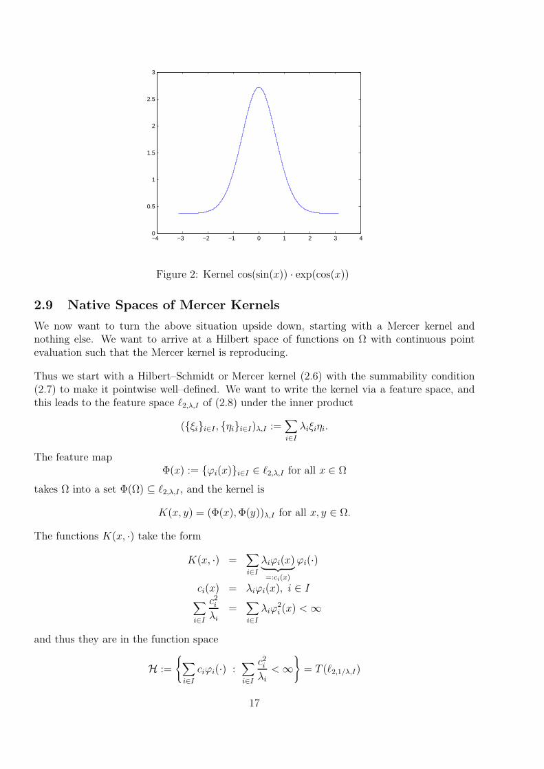
Figure 2: Kernel cos(sin(x)) · exp(cos(x))

2.9 Native Spaces of Mercer Kernels

We now want to turn the above situation upside down, starting with a Mercer kernel andnothing else. We want to arrive at a Hilbert space of functions on Ω with continuous pointevaluation such that the Mercer kernel is reproducing.

Thus we start with a Hilbert–Schmidt or Mercer kernel (2.6) with the summability condition(2.7) to make it pointwise well–defined. We want to write the kernel via a feature space, andthis leads to the feature space ℓ2,λ,I of (2.8) under the inner product

(ξii∈I , ηii∈I)λ,I :=∑

i∈I

λiξiηi.

The feature mapΦ(x) := ϕi(x)i∈I ∈ ℓ2,λ,I for all x ∈ Ω

takes Ω into a set Φ(Ω) ⊆ ℓ2,λ,I , and the kernel is

K(x, y) = (Φ(x),Φ(y))λ,I for all x, y ∈ Ω.

The functions K(x, ·) take the form

K(x, ·) =∑

i∈I

λiϕi(x)︸︷︷︸=:ci(x)

ϕi(·)

ci(x) = λiϕi(x), i ∈ I∑

i∈I

c2iλi

=∑

i∈I

λiϕ2i (x) <∞

and thus they are in the function space

H :=

∑

i∈I

ciϕi(·) :∑

i∈I

c2iλi<∞

= T (ℓ2,1/λ,I)

17

−4 −3 −2 −1 0 1 2 3 4

0.8

1

1.2

1.4

1.6

1.8

2

Figure 3: Kernel1− 1

2cos(x)

1−cos(x)+ 14

with the surjective (but not necessarily injective) linear map

T : ℓ2,1/λ,I → H, T (c) :=∑

i∈I

ciϕi.

Within this space, our pre–Hilbert space S = SΩ consists of all finite linear combinations

fa,X(y) =N∑

j=1

ajK(xj , y)

=N∑

j=1

aj

∑

i∈I

λiϕi(xj)ϕi(y)

=∑

i∈I

ϕi(y)λi

N∑

j=1

ajϕi(xj)

︸︷︷︸=:ci(a,X)

and the inner product is


j=1

N∑

k=1

ajbkK(xj , xk)

=∑

i∈I

1

λi

λi

M∑

j=1

ajϕi(xj)

(λi

N∑

k=1

bkϕi(xk)

)

=∑

i∈I

1

λici(a,X)ci(b, Y )

= (c(a,X), c(b, Y ))1/λ,I

if we define

c(a,X) := ci(a,X)i∈I =

λi

N∑

j=1

ajϕi(xj)

i∈I

∈ ℓ2,1/λ,I .

18

The native space NK for K is the completion of SΩ under this inner product, and it is a spaceof functions on Ω. By the above identity, it is clear that it is isometrically isomorphic to theHilbert subspace of ℓ2,1/λ,I obtained as the completion of the span of all c(a,X).

We want to relate the native space to a function subspace of H now. To this end, we can formthe closure of the span of all elements of Φ(Ω) in ℓ2,λ,I and denote it by Kλ,Ω. It clearly is aclosed subspace of ℓ2,λ,I and thus itself a Hilbert space. The elements c ∈ ℓ2,1/λ,I , when seen asfunctionals on ℓ2,λ,I , satisfy

(R(c),Φ(x))λ,I = c(Φ(x)) =∑

i∈I

ciϕi(x) = T (c)(x)

for all x ∈ Ω. A special case is

(R(c(a,X)),Φ(x))λ,I = fa,X(x),

and by definition of c(a,X) we also have R(c(a,X)) ∈ Kλ,Ω for all fa,X ∈ SΩ. This leads to

Theorem 2.32 The native space for a Mercer kernel on Ω with weights λi, i ∈ I and featuresϕi, i ∈ I is isometrically isomorphic to the space Hλ := T (R−1(Kλ,Ω)) ⊂ H if Hλ is equippedwith the inner product

(T (c), T (d))Hλ:=∑

i∈I

cidi

λi= (c, d)1/λ,I .

Proof: It is tempting to define the above bilinear form on all of H, but the representation offunctions in H in terms of coefficients of the ϕi is not unique, i.e. T is not necessarily injective.However, the representation is unique when restricted to the subspace Hλ ⊂ H. To see this,assume

T (c) =∑

i∈I

ciϕi =∑

j∈I

djϕj = T (d)

as functions in Hλ ⊂ H, i.e. with R(c), R(d) ∈ Kλ,Ω. Then

(R(c) − R(d),Φ(x))λ,I = (T (c) − T (d))(x) = 0

proving R(c) = R(d) as elements of Kλ,Ω and finally c = d due to bijectivity of the Riesz map.The rest follows from

(T (c(a,X)), T (c(b, Y )))Hλ= (c(a,X), cb, Y ))1/λ,I = (fa,X , fb,Y )K .

2

2.10 Finite Case

We now specialize to the context of learning models on a finite set Ω consisting of |Ω| pointsand a finite–dimensional feature space. Instead of using point notation for Ω, we can identifyΩ with the set Ω = 1, . . . , |Ω| and use index notation instead, and we assume the featurespace to be IRL for simplicity. Mercer kernels (2.6) then can be written as symmetric positivesemidefinite matrices K with entries Kr,s, 1 ≤ r, s ≤ |Ω| as

K = ΦΛΦT

19

with an L× L diagonal matrix Λ containing positive weights λ1, . . . , λL on its diagonal, whileΦ is a L× |Ω| matrix consisting of entries ϕi(r), 1 ≤ i ≤ L, 1 ≤ r ≤ |Ω|.

The space S = SΩ is then spanned by the |Ω| columns or rows of K, but we shall stick tocolumn notation when we consider a function on Ω. Each function f in S thus is a linearcombination of columns of K, and thus it has the form fa,Ω := Ka with a vector a ∈ IR|Ω|. Theinner product then is

(fa,Ω, fb,Ω)K = aTKb = aT ΦΛΦT b for all a, b ∈ IR|Ω|.

Our complicated proof of section 2.4 for the well–definedness of the inner product now takes asimpler form, since for Ka = Ka and Kb = Kb we get

(fa,Ω, fb,Ω)K = aTKb= aTKb

= aTKb= (fa,Ω, fb,Ω)K ,

but readers will see that the basic argument is the same. Also, the positive definiteness of theinner product is simple to see, because from ‖fa,Ω‖2

K = aTKa = 0 we first get ΦTa = 0 from

0 = aTKa = aT ΦΛΦTa = aT Φ√

Λ√

ΛΦTa = ‖√

ΛΦTa‖22

with the nonsingular diagonal matrix√

Λ defined in an obvious way. But ΦTa = 0 impliesfa,Ω = Ka = ΦΛΦTa = 0.

In practical cases, the matrices Φ and K are much too large to be handled, but there areefficient methods for the reduction of dimensions via principal component analysis orsingular value decomposition. We describe the basic principle now, but remark thatpractical applications will proceed differently.

A singular value decomposition splits K into a product

K = ΦΛΦT = UΣUT

with an orthogonal |Ω|× |Ω| matrix U and a diagonal |Ω|× |Ω| matrix Σ of singular values ofK, i.e. the nonnegative eigenvalues of KTK. Note that this amounts to consider an equivalentsetting with now L = |Ω|, U = Φ, and Λ = Σ, but now the diagonal of Σ may contain zeroentries. The orthogonal matrix U just is a coordinate change in the native space, and thus doesnot matter in theory. The problem thus behaves exactly as in the case K = Σ, i.e. as if thekernel was diagonal. We shall come back to the finite situation later.

2.11 Kernels for Univariate Sobolev Spaces

Let us calculate the kernel for Sobolev space Hk2 [a, b] for an interval [a, b] ⊂ IR. It has the inner

product

(f, g)k :=k∑

j=0

∫ b

af (j)(t)g(j)(t)dt =

k∑

j=0

(f (j), g(j)

)

L2[a,b]

20

and consists of all functions whose k–th derivative is in L2[a, b]. For k ≥ 1 these functions arecontinuous and have continuous point evaluation. To prove continuity, take a ≤ x ≤ y ≤ b toget

|f(x) − f(y)| ≤∫ y

x|f ′(t)|dt

≤√∫ y

x1dt

√∫ y

x|f ′(t)|2dt

≤ √y − x

√∫ b

a|f ′(t)|2dt

≤ √y − x‖f‖1.

Continuous point evaluation follows everywhere, if we have it at a and use the above argument.To prove it at a, just verify

f(a) =1

b− a

∫ b

af(t)dt+

1

b− a

∫ b

af ′(t)(t− b)dt

via integration by parts and bound it like we did above.

The kernel Kk of the space for k ≥ 1 must exist and should satisfy

f(x) =k∑

j=0

∫ b

af (j)(t)

∂jKk(x, t)

∂tjdt

for all x ∈ [a, b] and f ∈ Hk2 [a, b].

We only look at the case k = 1 and have to care for

f(x) =∫ b

af(t)K1(x, t)dt+

∫ b

af ′(t)K ′

1(x, t)dt

where from now on we keep x fixed and use only derivatives with respect to t. We want touse integration by parts on the second integral in order to generate the two other terms. Butthen we have to assume that K1(x, t) has a derivative discontinuity at t = x, and we split theintegral there. This yields

∫ ba f

′(t)K ′1(x, t)dt = [f(t)K ′(x, t)]xa −

∫ xa f(t)K ′′

1 (x, t)dt

+ [f(t)K ′(x, t)]bx −∫ bx f(t)K ′′

1 (x, t)dt

and we manage to get the reproduction formula if we can satisfy

K ′′1 (x, t) = K1(x, t) for all x, t

K ′1(x, a) = 0 for all x

K ′1(x, b) = 0 for all x

∂K1(x, t)

∂t |t=x−

= α(x) for all x

∂K1(x, t)

∂t |t=x+

= β(x) for all x

α(x) − β(x) = 1 for all x.

The differential equation K ′′1 (x, t) = K1(x, t) has the general solution

K1(x, t) = c+(x)e+t + c−(x)e−t

21

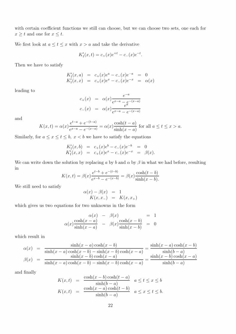
with certain coefficient functions we still can choose, but we can choose two sets, one each forx ≥ t and one for x ≤ t.

We first look at a ≤ t ≤ x with x > a and take the derivative

K ′1(x, t) = c+(x)e+t − c−(x)e−t.

Then we have to satisfy

K ′1(x, a) = c+(x)ea − c−(x)e−a = 0

K ′1(x, x) = c+(x)ex − c−(x)e−x = α(x)

leading to

c+(x) = α(x)e−a

ex−a − e−(x−a)

c−(x) = α(x)ea

ex−a − e−(x−a)

and

K(x, t) = α(x)et−a + e−(t−a)

ex−a − e−(x−a)= α(x)

cosh(t− a)

sinh(x− a)for all a ≤ t ≤ x > a.

Similarly, for a ≤ x ≤ t ≤ b, x < b we have to satisfy the equations

K ′1(x, b) = c+(x)eb − c−(x)e−b = 0

K ′1(x, x) = c+(x)ex − c−(x)e−x = β(x).

We can write down the solution by replacing a by b and α by β in what we had before, resultingin

K(x, t) = β(x)et−b + e−(t−b)

ex−b − e−(x−b)= β(x)

cosh(t− b)

sinh(x− b).

We still need to satisfyα(x) − β(x) = 1

K(x, x−) = K(x, x+)

which gives us two equations for two unknowns in the form

α(x) − β(x) = 1

α(x)cosh(x− a)

sinh(x− a)− β(x)

cosh(x− b)

sinh(x− b)= 0

which result in

α(x) =sinh(x− a) cosh(x− b)

sinh(x− a) cosh(x− b) − sinh(x− b) cosh(x− a)=

sinh(x− a) cosh(x− b)

sinh(b− a)

β(x) =sinh(x− b) cosh(x− a)

sinh(x− a) cosh(x− b) − sinh(x− b) cosh(x− a)=

sinh(x− b) cosh(x− a)

sinh(b− a)

and finally

K(x, t) =cosh(x− b) cosh(t− a)

sinh(b− a)a ≤ t ≤ x ≤ b

K(x, t) =cosh(x− a) cosh(t− b)

sinh(b− a)a ≤ x ≤ t ≤ b.

22

We leave it to the reader to go all the way backwards to prove the reproduction equation.

But we can also look at the case of Sobolev space on (−∞,∞). The kernel, as a function of t,then must have the form

K(x, t) = c+(x)et −∞ < t ≤ x <∞K(x, t) = c−(x)e−t −∞ < x ≤ t <∞

because otherwise it would not be integrable. To get continuity at t = x we need

c+(x)ex = c−(x)e−x

which is satisfied if we writec+(x) = c(x)e−x

c−(x) = c(x)e+x

with some function c(x). We have

K ′(x, t) = c+(x)et = c(x)et−x −∞ < t ≤ x <∞K ′(x, t) = −c−(x)e−t = −c(x)ex−t −∞ < x ≤ t <∞

and we can satisfy K ′(x, x−) −K ′(x, x+) = 1 by simply setting c(x) = 12. Thus

K(x, t) = 12et−x −∞ < t ≤ x <∞

K(x, t) = 12ex−t −∞ < x ≤ t <∞

or

K(x, t) =1

2e−|x−t| for all x, t ∈ IR,

see figure 4. The local kernel on [−1, 1] is in Figure 5.

−1 −0.8 −0.6 −0.4 −0.2 0 0.2 0.4 0.6 0.8 10.15

0.2

0.25

0.3

0.35

0.4

0.45

0.5Exponential Kernel for Sobolev Space

Figure 4: The kernel exp(−|x− y|)

23

Figure 5: The local kernel for W 12 [−1, 1]

Just for fun let us check if this occurs as the limit of the previous kernel for a → −∞ andb→ ∞. We just check the case


sinh(b− a)for all a ≤ t ≤ x ≤ b

and leave the other case to the reader. We get


sinh(b− a)

=1

2

(ex−b + eb−x)(et−a + ea−t)

eb−a − ea−b

=1

2

eb−a

eb−a

(ex−2b + e−x)(et + e2a−t)

1 − e2a−2b

→ 1

2e−xet =

1

2et−x

as required.

The upshot of all of this is to show that certain well–known and useful spaces have usefulreproducing kernels. But at other places we shall also show the opposite, i.e. that certainuseful kernels have useful native spaces.

3 Optimal Recovery

This section concerns the reconstruction of functions from native spaces from pointwise dataon subsets of Ω.

3.1 Optimality Properties

We now fix a finite set X = x1, . . . , xN ⊂ Ω and consider the finite–dimensional space

SX := span K(x, ·) : x ∈ X.

24

Such spaces are useful in various contexts, because they provide trial functions for approxi-mation and interpolation of functions, or the solution of differential equations. We first checkthe best approximations from SX to functions in the Native Space.

Theorem 3.1 Given an arbitrary function f from the native space NK of a positive semidefi-nite kernel K on a set Ω, fix a finite set X = x1, . . . , xN ⊂ Ω. Then the solution fa∗,X of thefinite–dimensional approximation problem

mins∈SX

‖f − s‖K = mina∈IRN

‖f − fa,X‖K

exists and is an interpolant to f on X. The coefficients solve the linear system

fa∗,X(xk) =N∑

j=1

a∗jK(xj , xk) = f(xk), 1 ≤ k ≤ N. (3.2)

Proof: From standard arguments of linear approximation in spaces with inner products itfollows that the solution exists and has the orthogonality property

(f − fa∗,X , s)K = 0 for all s ∈ SX

which includes

0 = (f − fa∗,X , K(xk, ·))K = f(xk) − fa∗,X(xk), 1 ≤ k ≤ N

due to the reproduction property (2.20). But this implies the rest of the proof. 2

Note that this guarantees that the linear system (3.2) with the kernel matrix AK,X,X is alwayssolvable, though the matrix may be singular. The matrix is only positive semidefinite, but theright–hand side of (3.2), being a set of values on X of a function from the native space, alwayslies in the span of the columns. The coefficients a∗j and the resulting function fa∗,X may not beunique unless the kernel is positive definite.

Theorem 3.3 Given an arbitrary function f from the native space NK of a positive semidefi-nite kernel K on a set Ω and a finite set X = x1, . . . , xN ⊂ Ω. Under all interpolants fromNK to f on X, the interpolating functions fa∗,X from the previous theorem minimize the nativespace norm, i.e.

ming∈INK , g=f on X

‖g‖K = ‖fa∗,X‖K .

Proof: We have to show‖g‖2

K ≥ ‖fa∗,X‖2K

for all g ∈ NK with g = f on X. But we can write

‖g‖2K = ‖fa∗,X + (g − fa∗,X)‖2

K

= ‖fa∗,X‖2K + 2(fa∗,X , g − fa∗,X)K + ‖g − fa∗,X‖2

K

25

and get the assertion from

(fa∗,X , g − fa∗,X)K =

N∑

j=1

a∗jK(xj , ·), g − fa∗,X

K

=N∑

j=1

a∗j (K(xj , ·), g − fa∗,X)K

=N∑

j=1

a∗j (g(xj) − fa∗,X(xj))

=N∑

j=1

a∗j (g(xj) − f(xj)) = 0

proving the theorem. 2

3.2 Lagrange Reformulation

We now fix K, X = x1, . . . , xN ⊂ Ω and a point x ∈ Ω. Then we define the functionfx(·) := K(x, ·) ∈ NK and carry the previous construction out for this function. Consequently,we get a solvable system of equations

N∑

j=1

u∗j(x)K(xj , xk) = K(xk, x), 1 ≤ k ≤ N, x ∈ Ω (3.4)

for each x ∈ Ω, and for reasons to become clear soon, we now denote the x–dependent solutioncoefficients by u∗j(x). In fact, this is the standard notation for a cardinal or Lagrange basis,and in case of nonsingularity of the kernel matrix we immediately see that the characteristicequations

u∗j(xk) = δj,k, 1 ≤ j, k ≤ N

for such a basis are satisfied.

If we only have positive semidefiniteness, we can still rewrite any solution fa∗,X of the originalproblem of interpolation or approximation of f on X in the form

.

fa∗,X(x) =N∑

k=1

a∗kK(xk, x)

=N∑

k=1

a∗k

N∑

j=1

u∗j(x)K(xj , xk)

=N∑

j=1

u∗j(x)N∑

k=1

a∗kK(xj , xk)

=N∑

j=1

u∗j(x)fa∗,X(xj)

=N∑

j=1

u∗j(x)f(xj)

(3.5)

which generalizes the usual Lagrange formulation of interpolation. Note that there still isnonuniqueness, but in our new form we have found a representation which separates the

26

influence of X and f . In particular, we can take an arbitrary f = fb,X ∈ SX for an arbitraryb ∈ IRN and conclude

fb,X(x) =N∑

j=1

u∗j(x)fb,X(xj).

Theorem 3.6 The linear quasi–interpolation operator

QX(f) :=N∑

j=1

u∗j(·)f(xj)

on the native space NK reproduces all functions from SX using only their values on X. Thepointwise error has the representation

f(x) −QX(f)(x) = (f,KX(x, ·))K for all x ∈ Ω

with the X–dependent power kernel

KX(x, y) := K(x, y) −N∑

j=1

u∗j(x)K(xj , y) for all x, y ∈ Ω

and the error bound

|f(x) −QX(f)(x)| ≤ ‖f‖KPX(x) for all x ∈ Ω (3.7)

with the power function

P 2X(x) := ‖KX(x, ·)‖2

K

= K(x, x) − 2N∑

j=1

u∗j(x)K(xj , x) +N∑

j,k=1

u∗j(x)u∗k(x)K(xj , xk).

(3.8)

Proof: Clearly, the definition of the quasi–interpolation operator and the reproduction equationimply

f(x) −QX(f)(x) = (f,K(x, ·))K −N∑

j=1

u∗j(x)(f,K(xj , ·))K

= (f,KX(x, ·))K for all x ∈ Ω.

2

Unfortunately, we cannot directly conclude that the functions u∗j are in the native space or inSX , because we have no invertibility of the kernel matrix.

To prove that we can choose the u∗j(x) in such a way that they lie in SX , we start a detour andask for the coefficients a1, . . . , aN which minimize

supf∈NK , ‖f‖K≤1

|f(x) −N∑

j=1

ajf(xj)|.

Clearly these coefficients, if they exist at all, will be dependent on x. We introduce the standardpoint–evaluation functional

δx : NK → IR, δx(f) = f(x) for all f ∈ NK

27

and consider its norm

‖δx‖K := supf∈NK , ‖f‖K≤1

|f(x)| = supf∈NK , ‖f‖K≤1

|(f,K(x, ·))K| ≤ ‖K(x, ·)‖K =√K(x, x)

where we also used the index K to indicate the norm in the dual of the native space. But if

we insert f := K(x, ·)/√K(x, x), we get equality above. Our minimization problem then turns

into

mina∈IRN

‖δx −N∑

j=1

ajδxj‖2

K = mina∈IRN

K(x, x) − 2N∑

j=1

ajK(x, xj) +N∑

j,k=1

ajakK(xj , xk)

. (3.9)

By standard least–squares arguments, or by simple differentiation we see that the necessaryequations in a minimum are

N∑

j=1

ajK(xk, xj) = K(x, xk), 1 ≤ k ≤ N

and they are satisfied if we take aj = u∗j(x) from (3.4). Thus we know that the minimumproblem is solved by what we had before, and get

Theorem 3.10 Let K be a positive semidefinite kernel on Ω, and let X = x1, . . . , xN ⊂ Ωbe a fixed set. For all points x ∈ Ω the coefficient functions u∗j(x) of (3.4) satisfy

infa∈IRN

supf∈NK , ‖f‖K≤1

|f(x) −N∑

j=1

ajf(xj)| = supf∈NK , ‖f‖K≤1

|f(x) −N∑

j=1

u∗j(x)f(xj)|,

i.e. they realize the optimal pointwise error for all interpolants. Furthermore, there is an errorbound

|f(x) −N∑

j=1

u∗j(x)f(xj)| ≤ ‖f‖KPX,K(x) for all x ∈ Ω, f ∈ NK (3.11)

with the power function defined as

P 2X,K(x) := ‖δx −

N∑

j=1

u∗j(x)δxj‖2

K

= K(x, x) − 2N∑

j=1


j,k=1

u∗j(x)u∗k(x)K(xj , xk)

= K(x, x) −N∑

j=1

u∗j(x)K(xj , x) for all x ∈ Ω

(3.12)

and with values which are independent of the choice of the u∗j(x) in case of nonuniqueness.

Proof: If the necessary equations for the minimum of a positive semidefinite finite–dimensionalquadratic form are satisfied somewhere, they are sufficient for a minimum. The location of theminimum may be nonunique, but the value is not. This proves the first assertion and the finalpart of the last. The middle part follows from the definition of the power function, and thesimplification between the third and last line follows from (3.4). 2

This result looks very theoretic, but it is of great practical importance, because the powerfunction for fixed X can be calculated explicitly everywhere in Ω, and the error bound (3.11)allows to estimate the error of all possible interpolants based on the data locations in X.

28

Corollary 3.13 In addition, the power function PX,K(x) always vanishes at the points of X.

Proof: Clearly, for x = xk the coefficients aj := δjk are admissible and lead to the value zero.Since the minimum value is unique (while the location of the minimum is not), we have theassertion in spite of the nonuniqueness of the solution. 2

3.3 Calculation

We now want to take a closer look at the systems (3.2) or (3.4). To this end, we perform asingular–value–decomposition of the kernel matrix as

A = UΣUT

with an orthogonal matrix U and a diagonal matrix with nonnegative entries σ1, . . . , σN . Wefocus on (3.9) as minimization of a quadratic form. The latter is

0 ≤ Q(a) = K(x, x) − 2N∑

j=1

ajK(x.xj) +N∑

j,k=1

ajakK(xj , xk)

= K(x, x) − 2aTKX(x) + aTAa withKX(x) := (K(x1, x), . . . , K(xN , x))

T

and can be rewritten as

Q(a) = K(x, x) − 2aTUUTKX(x) + aTUUTAUUTa= K(x, x) − 2aTU UTKX(x)︸︷︷︸

=:z(x)

+aTUΣUT a︸︷︷︸=:b

= R(b) := K(x, x) − 2bT z(x) + bT Σb

= K(x, x) +N∑

j=1

(b2jσj − 2bjzj(x)

).

We know that this quadratic form is always nonnegative, and we can minimize it now by takingderivatives with respect to each bj . The optimal values b∗j (x) have to satisfy

b∗j (x)σj = zj(x), 1 ≤ j ≤ N.

This leads to

b∗j (x) :=zj(x)

σj

for σj > 0.

In case of σj = 0 we must (in theory) have zj(x) = 0 because otherwise the quadratic formcould take on negative values. For these j we can take any b∗j (x), and we formally write

b∗j(x) :=

zj(x)

σj

σj > 0

λjzj(x) σj = 0

with arbitrary λj for the j with σj = 0. Thus we can write

b∗(x) = Dz(x)

29

with a diagonal matrix D = D(σ, λ) having the entries

1

σjfor σj > 0

λj for σj = 0

on the diagonal. This yields the representation

a∗(x) = Ub∗(x) = UDz(x) = UDUTKX(x)

of the total solution, but we already know that this solution also arises as u∗j(x) = a∗j (x) inthe system (3.4) and the Lagrange type formula (3.5). But in the above form we see that thesolution can in spite of the singular system be written in such a way that it lies in SX and thusin the native space.

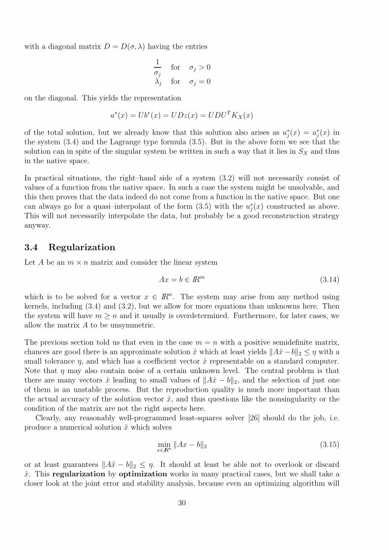
In practical situations, the right–hand side of a system (3.2) will not necessarily consist ofvalues of a function from the native space. In such a case the system might be unsolvable, andthis then proves that the data indeed do not come from a function in the native space. But onecan always go for a quasi–interpolant of the form (3.5) with the u∗j(x) constructed as above.This will not necessarily interpolate the data, but probably be a good reconstruction strategyanyway.

3.4 Regularization

Let A be an m× n matrix and consider the linear system

Ax = b ∈ IRm (3.14)

which is to be solved for a vector x ∈ IRn. The system may arise from any method usingkernels, including (3.4) and (3.2), but we allow for more equations than unknowns here. Thenthe system will have m ≥ n and it usually is overdetermined. Furthermore, for later cases, weallow the matrix A to be unsymmetric.

The previous section told us that even in the case m = n with a positive semidefinite matrix,chances are good there is an approximate solution x which at least yields ‖Ax− b‖2 ≤ η with asmall tolerance η, and which has a coefficient vector x representable on a standard computer.Note that η may also contain noise of a certain unknown level. The central problem is thatthere are many vectors x leading to small values of ‖Ax − b‖2, and the selection of just oneof them is an unstable process. But the reproduction quality is much more important thanthe actual accuracy of the solution vector x, and thus questions like the nonsingularity or thecondition of the matrix are not the right aspects here.

Clearly, any reasonably well-programmed least-squares solver [26] should do the job, i.e.produce a numerical solution x which solves

minx∈IRn

‖Ax− b‖2 (3.15)

or at least guarantees ‖Ax − b‖2 ≤ η. It should at least be able not to overlook or discardx. This regularization by optimization works in many practical cases, but we shall take acloser look at the joint error and stability analysis, because even an optimizing algorithm will

30

recognize that it has problems to determine x reliably if columns of the matrix A are close tobeing linearly dependent.

By singular-value decomposition [26], the matrix A can be decomposed into

A = UΣV T (3.16)

where U is an m×m orthogonal matrix, Σ is an m× n matrix with zeros except for singularvalues σ1, . . . , σn on the diagonal, and where V T is an n× n orthogonal matrix. Due to somesophisticated numerical tricks, this decomposition can under normal circumstances be donewith O(mn2 + nm2) complexity, though it needs an eigenvalue calculation. One can assume

σ21 ≥ σ2

2 ≥ . . . ≥ σ2n ≥ 0,

and the σ2j are the nonnegative eigenvalues of the positive semidefinite n× n matrix ATA.

The condition number of the non-square matrix A is then usually defined to be σ1/σn. Thisis in line with the usual spectral condition number ‖A‖2‖A−1‖2 for the symmetric casem = n. The numerical computation of U and V usually is rather stable, even if the totalcondition is extremely large, but the calculation of small singular values is hazardous. Thusthe following arguments can rely on U and V , but not on small singular values.

Using (3.16), the solution of either the minimization problem (3.15) or, in the case m = n,the solution of (3.14) can be obtained and analyzed as follows. We first introduce new vectors

c := UT b ∈ IRm and y := V Tx ∈ IRn

by transforming the data and the unknowns orthogonally. Since orthogonal matrices preserveEuclidean lengths, we rewrite the squared norm as

‖Ax− b‖22 = ‖UΣV Tx− b‖2

2

= ‖ΣV Tx− UT b‖22

= ‖Σy − c‖22

=n∑

j=1

(σjyj − cj)2 +

m∑

j=n+1

c2j

where now y1, . . . , yn are variables. Clearly, the minimum exists and is given by the equations

σjyj = cj , 1 ≤ j ≤ n,

but the numerical calculation runs into problems when the σj are small and imprecise in absolutevalue, because then the resulting yj will be large and imprecise. The final transition to thesolution x = V y by an orthogonal transformation does not improve the situation.

If we assume existence of a good solution candidate x = V y with ‖Ax− b‖2 ≤ η, we have

n∑

j=1

(σj yj − cj)2 +

m∑

j=n+1

c2j ≤ η2. (3.17)

A standard regularization strategy to construct a reasonably stable approximation y is tochoose a positive tolerance ǫ and to define

yǫj :=

cj

σj|σj| ≥ ǫ

0 |σj| < ǫ

31

i.e. to ignore small singular values, because they are usually polluted by roundoff and hardlydiscernible from zero. This is called the truncated singular value decomposition (TSVD).Fortunately, one often has small c2j whenever σ2

j is small, and then chances are good that

‖Axǫ − b‖22 =

∑

1 ≤ j ≤ n|σj | ≥ ǫ

c2j +m∑

j=n+1

c2j ≤ η2

holds for xǫ = V yǫ.

0 50 100 150 200 250 300 350 400 450−18

−16

−14

−12

−10

−8

−6

−4

−2

0

2

Number of DOF

Log of linear system error−log of condition of subsystem

Figure 6: Error and condition of linear subsystems via SVD

Figure 6 is an example interpolating the MATLAB peaks function in m = n = 441 regularpoints on [−3, 3]2 by Gaussians with scale 1, using the standard system (3.2). Following afixed 441 × 441 singular value decomposition, we truncated after the k largest singular values,thus using only k degrees of freedom (DOF). The results for 1 ≤ k ≤ 441 show that there arelow-rank subsystems which already provide good approximate solutions.

But now we proceed with our analysis. In case of large cj for small σj , truncation isinsufficient, in particular if the dependence on the unknown noise level η comes into focus. Atleast, the numerical solution should not spoil the reproduction quality guaranteed by (3.17),which is much more important than an exact calculation of the solution coefficients. Thus onecan minimize ‖y‖2

2 subject to the essential constraint

n∑

j=1

(σjyj − cj)2 +

m∑

j=n+1

c2j ≤ η2, (3.18)

but we suppress details of the analysis of this optimization problem. Another, more popularpossibility is to minimize the objective function

n∑

j=1

(σjyj − cj)2 + δ2

n∑

j=1

y2j

32

10−25

10−20

10−15

10−10

10−5

100

10−9

10−8

10−7

10−6

10−5

10−4

10−3

10−2

10−1

100

Delta

Err

or

Error without noiseError with 0.01% noise

Figure 7: Error as function of regularization parameter δ2

where the positive weight δ allows to put more emphasis on small coefficients if δ is increased.This is called Tikhonov regularization.

The solutions of both settings coincide and take the form

yδj :=

cjσj

σ2j + δ2

, 1 ≤ j ≤ n

depending on the positive parameter δ of the Tikhonov form, and for xδ := V yδ we get

‖Axδ − b‖22 =

n∑

j=1

c2j

(δ2

δ2 + σ2j

)2

+m∑

j=n+1

c2j ,

which can me made smaller than η2 for sufficiently small δ. The optimal value δ∗ of δ for aknown noise level η in the sense of (3.18) would be defined by the equation ‖Axδ∗ − b‖2

2 = η2,but since the noise level is only rarely known, users will be satisfied to achieve a tradeoffbetween reproduction quality and stability of the solution by inspecting ‖Axδ − b‖2

2 for varyingδ experimentally.

We now repeat the example leading to Figure 6, replacing the truncation strategy by theabove regularization. Figure 7 shows how the error ‖Axδ −b‖∞,X depends on the regularizationparameter δ. In case of noise, users can experimentally determine a good value for δ even for anunknown noise level. The condition of the full matrix was calculated by MATLAB as 1.46 ·1019,but it may actually be higher. Figure 8 shows that the coefficients |cj| are indeed rather smallfor large j, and thus regularization by truncated SVD will work as well in this case.

From Figures 8 and 7 one can see that the error ‖Axδ − b‖ takes a sharp turn at the noiselevel. This has led to the L-curve method for determining the optimal value of δ, but theL-curve is defined differently as the curve

δ 7→ (log ‖yδ‖22, log ‖Axδ − b‖2

2).

The optimal choice of δ is made where the curve takes its turn, if it does so, and there arevarious way to estimate the optimal δ, see [27, 28, 29] including a MATLAB software package.

33

0 50 100 150 200 250 300 350 400 45010

−14

10−12

10−10

10−8

10−6

10−4

10−2

100

102

j

Rat

io

c coefficients for data without noisec coefficients for data with 0.01% noise

Figure 8: Coefficients |cj | as function of j

Figure 9 shows the typical L-shape of the L-curve in case of noise, while in the case of exactdata there is no visible sharp turn within the plot range. The background problem is the sameas for the previous figures.

Consequently, users of kernel techniques are strongly advised to take some care whenchoosing a linear system solver. The solution routine should incorporate a good regularizationstrategy or at least automatically project to stable subspaces and not give up quickly due tobad condition. Further examples for this will follow in later chapters.

But for large systems, the above regularization strategies are debatable. A singular-valuedecomposition of a large system is computationally expensive, and the solution vector willusually not be sparse, i.e. the evaluation of the final solution at many points is costly. In manycases, linear systems arising from kernels often have good approximate solutions with onlyfew nonzero coefficients, and the corresponding numerical techniques are other, and possiblypreferable regularizations which still are under investigation.

4 Conditionally Positive Definite Kernels

So far, we looked at positive semidefinite symmetric kernels. But this is not the end of the story.We need the more general notion of conditional positive (semi–) definite kernels, and there areseveral ways to introduce them. They do not fall directly out of a simple (non–distributional)Hilbert space setting, because otherwise they would be unconditionally positive semidefinite.Instead, the most important conditionally positive definite kernels like the thin–plate splineK(x, y) = log(‖x− y‖2

2) arise directly from applications, or as certain fundamental solutions ofpartial differential equations. Thus we have to begin with kernels first and then work our waytowards a Hilbert space.

We start with the most important univariate function class leading to conditionally positivedefinite kernels, i.e. the standard polynomial splines.

34

10−5

100

105

1010

1015

1020

10−18

10−16

10−14

10−12

10−10

10−8

10−6

10−4

10−2

100

L−curve for data without noiseL−curve for data with 0.01% noise

Figure 9: The L-curve for the same problem

4.1 Splines

The following is a somewhat nonstandard introduction to splines, modeled for extensions togeneral multivariate kernel-based function spaces.

First we fix a positive integer k and denote the space of real–valued polynomials with order(= degree -1) at most k by IP k. In the d–variate case we shall use the notation IP d

k.

4.1.1 Semi–inner product

As a function space, we use the vector space Ck[a, b] of all real-valued functions f with piecewisecontinuous k-th derivatives for which

|f |2k :=∫ b

a

(dkf(t)

dtk

)2

dt (4.1)

is finite. We leave it to the reader that this defines a reasonable vector space of functions on[a, b].

Equation (4.1) defines a semi-norm, i.e. it has the properties of a norm except for thedefiniteness, and there is a semi-inner product

(f, g)k :=∫ b

a

dkf(t)

dtkdkg(t)

dtkdt.

Lemma 4.2 The seminorm |f |k is zero if and only if f is a polynomial of order at most k.

Proof: Clearly, the seminorm |f |k is zero if f is a polynomial of order at most k. Conversely, ifthe seminorm |f |k is zero for some function f ∈ Ck[a, b], then f (k) is zero except for its points ofdiscontinuity. Then f consists of polynomial pieces of order at most k which are glued togetherin such a way that the (k−1)st derivative still is continuous. But then f is a global polynomialof order at most k. 2

35

4.1.2 Taylor’s Formula

We want to align the above starting point with what we know about positive semidefinite kernelsand reproducing kernel Hilbert spaces, but so far we have no inner product and no kernel. Butwe can go for a reproduction property which everybody should be well acquainted with.

Every function f on [a, b] with k continuous derivatives satisfies

f(x) =k−1∑

j=0

f (j)(a)

j!(x− a)j +

∫ x

af (k)(t)

(x− t)k−1

(k − 1)!dt, x ∈ [a, b]

and this generalizes to functions in Ck[a, b] (without proof here). This is a reproduction formula,and in the integral we can see what could later be a kernel, but we still have to work a little.

The upper bound x of the integral can be eliminated by defining the truncated power as

(z)k+ :=

zk z > 00 z < 012

z = 0, k = 00 else

to get

f(x) =k−1∑

j=0

f (j)(a)

j!(x− a)j +

∫ b

af (k)(t)

(x− t)k−1+

(k − 1)!dt, x ∈ [a, b].

With the kernel function

Kk(x, t) := (−1)k (x− t)2k−1+

(2k − 1)!

the above equation takes the form

f(x) =k−1∑

j=0

f (j)(a)

j!(x− a)j

︸︷︷︸=:(Pkf)(x)

+(f,Kk(x, ·))k

= (Pkf)(x) + (f,Kk(x, ·))k, x ∈ [a, b].

(4.3)

This is a reproduction formula, i.e. it allows f to be reproduced from f (k) in [a, b] and thederivatives at a up to order k − 1. We also have a kernel now, but it is unsymmetric, and thusit does not fit into our framework.

4.1.3 Taylor’s Formula Symmetrized

But note that we have tackled a symmetric problem in an unsymmetric way, which is amathematical crime. We should also use Taylor’s formula at b. This is

f(x) =k−1∑

j=0

f (j)(b)

j!(x− b)j +

∫ x

bf (k)(t)

(x− t)k−1

(k − 1)!dt, x ∈ [a, b]

=: (Qkf)(x) +∫ b

xf (k)(t)(−1)k (t− x)k−1

(k − 1)!dt

= (Qkf)(x) +∫ b

af (k)(t)(−1)k (t− x)k−1

+

(k − 1)!dt.

36

To get something symmetric, we take the mean of the two Taylor formulae. This is

f(x) = 12(Pkf)(x) + 1

2(Qkf)(x)

+12

∫ b

af (k)(t)

((x− t)k−1

+

(k − 1)!+ (−1)k (t− x)k−1

+

(k − 1)!

)dt

=: (Rkf)(x) + (f,Φk(x, ·))k

(4.4)

with(Rkf)(x) := 1

2(Pkf)(x) + 1

2(Qkf)(x)

=1

2

k−1∑

j=0

f (j)(a)

j!(x− a)j +

1

2

k−1∑

j=0

f (j)(b)

j!(x− b)j

Φk(x, t) := 12(−1)k |x− t|2k−1

(2k − 1)!.

To see that the form of the new symmetric kernel Φk is correct, we take its k-th derivative withrespect to t for the two cases

Φk(x, t) = 12(−1)k (x− t)2k−1

(2k − 1)!x ≥ t

Φk(x, t) = 12(−1)k (t− x)2k−1

(2k − 1)!t ≥ x

and get

dk

dtk12(−1)k (x− t)2k−1

(2k − 1)!= 1

2

(x− t)k−1

(k − 1)!x ≥ t

dk

dtk12(−1)k (t− x)2k−1

(2k − 1)!= 1

2(−1)k (t− x)k−1

(k − 1)!t ≥ x

where we can add the + subscript in both cases in order to arrive at (4.4).

Note that the two reproduction formulae (4.3) and (4.4) can both be used to our convenience.The different kernels are linked to different polynomial projectors.

4.1.4 Smoothest Interpolation

We assume M points x1 < x2 < · · · < xM in [a, b] ⊂ IR and corresponding real values y1, . . . , yM

to be given, and we want to find a function s∗ ∈ Ck[a, b] which minimizes |s|2k under all functionss ∈ Ck[a, b] satisfying the interpolation conditions

s(xj) = yj, 1 ≤ j ≤M.

Note that this is a somewhat more specific case of Theorem 3.3.

In contrast to standard polynomial interpolation, we keep the smoothness k fixed and allowvery large numbers M of data points, asking for the “smoothest” possible interpolant. Notethat this is an infinite-dimensional quadratic optimization problem with linear constraints. Butwe shall not plunge deeply into optimization here and try to solve the problem single-handed.

If the data are values p(xj) = yj of a polynomial p ∈ IP k, the solution obviously is p with|p|k = 0. To assure uniqueness of interpolation even in such a simple case, we need theadditional assumption M ≥ k.

37

We shall not directly prove the existence of a smoothest interpolant s∗. Instead, we first assumeit exists, then derive its necessary form, and finally prove that it can be numerically calculatedin its necessary (and simplified) form, proving existence constructively.

If s∗ is our “smoothest” interpolant, we now repeat the “parabola argument” used for provingthe characterization of best approximants in Euclidean spaces. Take any real number λ andany function v ∈ Ck[a, b] with v(xj) = 0, 1 ≤ j ≤M . Then for all such λ and v we have

|s∗ + λv|2k = |s∗|2k + 2λ(s∗, v)k + λ2|v|2k≥ |s∗|2k

and this implies

(s∗, v)k = 0 for all v ∈ Ck[a, b] with v(xj) = 0, 1 ≤ j ≤M. (4.5)

This argument can be put upside down and proves that any interpolating function s∗ with (4.5)must be a smoothest interpolant.

If we define the linear data map T : Ck[a, b] → IRM with

Tv := (v(x1), . . . , v(xM)), v ∈ Ck[a, b],

and the linear functional µ∗(v) := (s∗, v)k, the property (4.5) is

µ∗(v) = 0 for all v ∈ Ck[a, b] with T (v) = 0.

But then there is a vector α ∈ IRM with

µ∗(v) = αTT (v) for all v ∈ Ck[a, b].

This is a standard argument of linear algebra, see Lemma 9.10 in the Hilbert Space section. Itapplies since T is surjective and thus the range IRM = T (Ck[a, b]) is isomorphic to the quotient

space via Ck[a, b]/ker TQ→ T (Ck[a, b]). Since it vanishes on ker T , the functional µ∗ can be

safely defined on the quotient space and thus be written via the range of T as µ∗ = Qα = αTT .We now know that

(s∗, v)k = αTT (v) =M∑

j=1

αjv(xj) (4.6)

holds for all v ∈ Ck[a, b], and we insert (4.3) to get

(s∗, v)k =M∑

j=1

αj ((Pkv)(xj) + (v,Kk(xj, ·))k)

=M∑

j=1

αj(Pkv)(xj) + (v,M∑

j=1

αjKk(xj , ·))k

(s∗ −M∑

j=1

αjKk(xj , ·), v)k =M∑

j=1

αj(Pkv)(xj).

If we replace v in (4.6) by Pkv, we see that

0 = (s∗, Pkv)k = αTT (Pkv) =M∑

j=1

αjPkv(xj)

38

for all v ∈ Ck[a, b]. Since Pk clearly is surjective, this implies

M∑

j=1

αjq(xj) = 0 for all q ∈ IP k. (4.7)

Furthermore,

0 = (s∗ −M∑

j=1

αjKk(xj, ·), v)k

for all v ∈ Ck[a, b]. For the special case

v := p := s∗ −M∑

j=1

αjKk(xj , ·)

Lemma 4.2 now implies that p is a polynomial in IP k. This proves the first part of

Theorem 4.8 The “smoothest” interpolant s∗, if it exists, has the form

s∗ = p+M∑

j=1

αjKk(xj , ·) (4.9)

with a polynomial p ∈ IP k and M coefficients α1, . . . , αM satisfying (4.7). Conversely, if afunction s∗ of the form (4.9) with (4.7) interpolates the data, it is the “smoothest” interpolant.

Proof of the converse: Just follow the above argument backwards to arrive at the “parabolaargument”. Details are left to the reader. 2

Note that exactly the same argument works when using the symmetric kernel Φk instead of Kk.

4.1.5 Primitive Construction

We still have to prove that the “smoothest interpolant” exists. But since we now know whatit should look like, we prove existence constructively. But please keep in mind that there arebetter algorithms to construct the solution, given in treatises devoted to splines, e.g. Carl deBoor’s Practical Guide to Splines [16].

If we introduce a basis p1, . . . , pk for IP k, we can write the candidate for a smoothest interpolantas

s∗ :=M∑

j=1

αjKk(xj , ·) +k∑

ℓ=1

βℓpℓ

with the additional conditions (4.7) in the form

M∑

j=1

αjpℓ(xj) = 0, 1 ≤ ℓ ≤ k.

Again, the following argument works similarly for the symmetric kernel Φk instead of Kk.

Together with the usual interpolation conditions

s∗(xi) =M∑

j=1

αjKk(xj , xi) +k∑

ℓ=1

βℓpℓ(xi) = yi, 1 ≤ i ≤M

39

we get the (M + k) × (M + k) block system

(A PP T 0ℓ×ℓ

)(αβ

)=(y0ℓ

)(4.10)

with the matrices and vectors

A := (Kk(xj , xi))1≤i,j≤M

P := (pℓ(xi))1≤i≤M, 1≤ℓ≤k

yT := (y1, . . . , yM).

Theorem 4.11 If M ≥ k holds, the system (4.10) is uniquely solvable.

Proof: We show that the homogeneous system has only the trivial solution. Assume that ahomogeneous solution is given by vectors α ∈ IRM and β ∈ IRk. We then define s∗ and p as inthe above argument and see that s∗ is the smoothest interpolant to zero data. Since the zerofunction also does the job, we necessarily have |s∗|k = 0 and s∗ ∈ IP k. But since s∗ interpolateszero in M ≥ k points, it must be zero everywhere.

Then, for every v ∈ Ck[a, b] we have

0 = (s∗, v)k

= 0 +

M∑

j=1

αjKk(xj, ·), v

k

=M∑

j=1

αj (Kk(xj , ·), v)k

=M∑

j=1

αj (v(xj) − (Pkv)(xj))

=M∑

j=1

αjv(xj)

due to (4.7). By picking some useful v, e.g. as Lagrange interpolating polynomials, we getthat all αj must vanish. But the remaining equations then are Pβ = 0 and imply that thepolynomial

p :=k∑

ℓ=1

βℓpℓ

vanishes at all M ≥ k data points. Thus its coefficients must all be zero. 2

4.1.6 Properties

From Theorem 4.8 and equation (4.9) we see that the smoothest interpolant is of the form

s∗(x) =k∑

ℓ=1

βℓpℓ(x) +M∑

j=1

αj(xj − x)2k−1+

or, equivalently, but with different coefficients,

s∗(x) =k∑

ℓ=1

βℓpℓ(x) +M∑

j=1

αj |xj − x|2k−1+

40

with the additional conditions (4.7). Thus it is a piecewise polynomial of order at most 2k with“breakpoints” or “knots” at the data locations xj . It still has 2k − 2 continuous derivatives,which is roughly twice the smoothness originally postulated in the space Ck[a, b] except fork = 1 and k = 2.

Furthermore, the first form tells us that it is a polynomial of order at most k in [a, x0]. Sincethe equivalent second form is symmetric, we conclude in general that s∗ is a polynomial of orderat most k outside the data locations.

Altogether, the conditions

1. s∗ interpolates in x0 < . . . < xM in [a, b] and

2. is a C2k−2 function

3. consisting of polynomials of order at most 2k in each data interval [xj , xj+1] and

4. a polynomial of order at most k outside [x0, xM ]

uniquely define the solution to our problem, which is traditionally called the “natural interpo-lating spline of order 2k”.

4.1.7 Symmetrization

In view of multivariate kernel–based methods, we take a closer look at the symmetric kernelΦk. In particular,

(Φk(x, ·),Φk(y, ·))k = Φk(x, y) − (RkΦk(x, ·))(y)

and due to symmetry of the two other parts of the above identity,

(RkΦk(x, ·))(y) = (RkΦk(y, ·))(x).Lemma 4.12 If M ≥ k holds, and if formed with Φk, the matrix A defines a quadratic formwhich is positive definite on the subspace of vectors α ∈ IRM with (4.7).

Proof: The quadratic form defined by A and taken on the vectors α ∈ IRM with (4.7) is

αTAα =M∑

i=0

M∑

j=0

αiαjΦk(xi, xj)

=M∑

i=0

M∑

j=0

αiαj(Φk(xi, ·),Φk(xj , ·))k + 0

=

M∑

i=0

αiΦk(xi, ·),M∑

j=0

αjΦk(xj , ·)

k

=

∣∣∣∣∣

M∑

i=0

αiΦk(xi, ·)∣∣∣∣∣

2

k

≥ 0

and thus positive semidefinite. If it vanishes, then

p(x) :=M∑

i=0

αiΦk(xi, x)

41

must be a polynomial in IP k. With the same argument as in the proof of Theorem 4.11, nowtaking p instead of s∗, we get that all αi must vanish if (4.7) holds. 2

Definition 4.13 A kernel with the property described by Lemma 4.12 for all matrices arisingon M ≥ k points is called conditionally positive definite of order k.

This property will come up later in multivariate settings. But we can also push symmetrysomewhat further by defining the symmetric kernel

Ψk(x, y) := Φk(x, y) − (RkΦk(x, ·))(y)

which satisfies(Ψk(x, ·),Ψk(y, ·))k = Ψk(x, y) for all x, y ∈ [a, b] (4.14)

because we only modified Φ by a polynomial. The kernel matrix defined by Ψ instead of Φ alsois conditionally positive definite of order k. This follows from the above proof, but with theadditional step that if

p(x) :=M∑

i=0

αiΨk(xi, x)

is a polynomial, thenM∑

i=0

αiΦk(xi, x)

is also a polynomial, since the two differ only by a polynomial. The rest is as above. But thereis more:

Theorem 4.15 The kernel Ψk is both conditionally positive definite of order k and uncondi-tionally positive semidefinite.

Proof: This is an elementary consequence of (4.14). 2

Altogether, this sets the stage for conditional positive definiteness along the lines of Lemma4.12 and Definition 4.13.

4.1.8 Kernel Regularization

In the above situation, we can take the k + 1 polynomials pℓ(t) := tℓ−1 for 1 ≤ ℓ ≤ k + 1 =:Q = dim IP k for defining an extended kernel in “Mercer style” as

Kk(x, y) := Φk(x, y) +Q∑

ℓ=1

pℓ(x)pℓ(y),

where we also could replace Φk by Ψk. We shall later show that this trick leads to anunconditionally positive definite kernel in the spline situation.

42

Kernel φ(r), r = ‖x− y‖2 Order Conditions Name

(−1)⌈β/2⌉(c2 + r2)β/2 ⌈β/2⌉ β > 0, β /∈ 2IN Multiquadrics

(−1)⌈β/2⌉rβ ⌈β/2⌉ β > 0, β /∈ 2IN polyharmonic splines(−1)k+1r2k log r k + 1 k ∈ IN thin–plate splines

Table 1: Orders of conditional positive definiteness

4.1.9 Other Cases

We saw that spline theory leads to univariate conditionally positive definite kernels. But thereare other cases, in particular multivariate ones which we shall handle in detail later. Theseare radial kernels K(x, y) = φ(‖x− y‖2) with scalar functions φ : [0.∞) → IR and orders ofconditional positive definiteness given by Table 1.

Like the special spline kernels, such kernels arise naturally and are not directly identifiable asreproducing kernels of certain Hilbert spaces, because otherwise they would be unconditionallypositive semidefinite. Thus they have no direct link to Hilbert space theory, and we have torepeat the construction of sections 2.4 and 2.6 to see their connection to Hilbert spaces.

4.2 General Case

To define a sufficiently general notion of conditional positive (semi–) definiteness, we fix afinite–dimensional space IP of functions on a set Ω, denote its dimension by Q and select abasis p1, . . . , pQ.

Definition 4.16 A subset X = x1, . . . , xN of Ω is called IP–unisolvent, if zero is the onlyfunction in IP that vanishes on X.

This means that functions from IP are completely determined by their values on unisolvent setsX, and it implies that X must have at least Q elements for this to work. Therefore Ω musthave at least Q points, because otherwise the dimension of IP as a space of functions on Ω couldnot be Q. From now on, all subsets X of Ω we shall only consider must be IP–unisolvent andthus have at least Q points. Furthermore, to exclude certain degenerate situations, we assumeΩ to admit at least one unisolvent set and at least one additional point. Otherwise, we couldget away working with IP alone.

Definition 4.17 Let a finite–dimensional space IP of real–valued functions on a set Ω be given.A symmetric kernel K : Ω×Ω → IR is called IP–conditionally positive (semi–) definite,if for all IP–unisolvent subsets X = x1, . . . , xN of Ω the kernel matrices AK,X,X with entriesK(xj , xk), 1 ≤ j, k ≤ N ≥ Q are positive (semi–) definite on the subspace of IRN of vectorsa ∈ IRN with the moment conditions

N∑

j=1

ajp(xj) = 0 for all p ∈ IP . (4.18)

For notational convenience, we also define the N ×Q matrices PX by

PX := (pℓ(xj))1≤j≤N, 1≤ℓ≤Q

and note that these have rank Q for IP–unisolvent sets X. Furthermore, the moment conditions4.18 on a vector a ∈ IRN have the form P T

Xa = 0.

43

We now describe a general technique for the recovery of functions from data on unisolvent stesX, as we did for splines in (4.10).

Theorem 4.19 If K is a IP–conditionally positive definite kernel on Ω, the (N+Q)×(N+Q)matrices

AK,X,X,IP :=(AK,X,X PX

P TX 0Q×Q

)

withAK,X,X = (K(xk, xk))1≤j,k≤N

are nonsingular for each IP–unisolvent finite set X ⊆ Ω.

Proof: Consider a solution (aT , bT )T of the linear homogeneous system

(AK,X,X PX

P TX 0Q×Q

)(ab

)=(

0N×1

0Q×1

).

Then P TXa = 0 and AK,X,Xa + PXb = 0, leading to

0 = aT (AK,X,Xa+ PXb) = aTAK,X,Xa

and a = 0 due to P TXa = 0 and the definition of conditional positive definiteness. But then

PXb = 0, and unisolvence implies b = 0. 2

We now proceed like in the positive semidefinite case and set up the system(AK,X,X PX

P TX 0Q×Q

)(u∗(x)v∗(x)

)=(KX(x)p(x)

)(4.20)

with vectors

KX(x) := (K(x, x1), . . . , K(x, xN ))T , p(x) := (p1(x), . . . , pQ(x))T

for all x ∈ Ω. The system is solvable, and thus we get functions with

u∗(x) = (u∗1(x), . . . , u∗N(x))T , v∗(x) = (v∗1(x), . . . , v

∗Q(x))T , x ∈ Ω

which are in the space

SIP ,X := span (K(xj , ·) : xj ∈ X ∪ p1, . . . , pQ) . (4.21)

Specializing to the first N columns of the system and using unique solvability, we get

u∗j(xk) = δjk, 1 ≤ j, k ≤ N, v∗ℓ (xk) = 0, 1 ≤ ℓ ≤ Q, 1 ≤ k ≤ N. (4.22)

These Lagrange conditions lead us to define the interpolation operator

QX(f)(x) :=N∑

j=1

u∗j(x)f(xj)

which acts linearly on all functions f which have values on X and provides an interpolatingfunction from the space SIP ,X . The system also implies P T

Xu(x) = p(x), and this is

pℓ(x) =N∑

j=1

u∗j(x)pℓ(xj) = QX(pℓ)(x), 1 ≤ ℓ ≤ Q

44

and means that the functions from IP are reproduced by QX . But the range of QX cannot havea dimension larger than N , while the space SIP ,X is spanned by N +Q functions. To see thatQX maps to the subspace

SIP ,X := IP + aTKX(·) : P TXa = 0, a ∈ IRN (4.23)

of SIP ,X with additional moment conditions, we write the inverse of AK,X,X,IP in the form

(B RRT S

)

and get the equationsu(x) = BKX(x) + Rp(x)v(x) = RTKX(x) + Sp(x)BPX = 0

proving that the rows of B satisfy the moment conditions via

P TX(eT

j B)T = (eTj BPX)T = 0, 1 ≤ j ≤ N.

Therefore, the interpolation operator must necessarily have the alternative form

QX(f)(x) :=N∑

j=1

aj(f)K(xj , x) +Q∑

ℓ=1

bℓ(f)pℓ(x) (4.24)

with P TXa(f) = 0 since the result lies in SIP ,X . The coefficients solve the system

(AK,X,X PX

P TX 0Q×Q

)(a(f)b(f)

)=(fX

0

)(4.25)

with fX := (f(x1), . . . , f(xN))T , and this is how the interpolant is calculated in practice.

We note some facts we need later:

Lemma 4.26 1. In (4.23), the sum is direct, i.e. there is no nonzero function in IP whichcan be written in the form aTKX(x) with a unisolvent set X.

2. The dimension of SIP ,X is N .

3. Both operators QX and Id−QX are projectors, i.e. they are linear and idempotent.

Proof of the lemma: The representation (4.24) of the interpolation operator via the solutionof the system (4.25) is unique. A function in IP , when written as its own interpolant, thuscoincides with the right–hand sum, and thus the first sum must be zero, proving the firstassertion.

The second follows similarly: each function in SIP ,X has exactly the form (4.24) and satisfies thesystem (4.25) with its own values on X in the right–hand side. Providing N arbitrary valueson the right–hand side will produce a function in SK,X , and the corresponding map is bijectivedue to nonsingularity of the matrix. Thus the space spanned by the solution coefficients, andthus also the space SIP ,X are isomorphic to IRN . The third assertion follows from the Lagrangeproperty (4.22). 2

45

4.3 Inner Products

There are many ways to construct a “native” Hilbert space when starting from a IP–conditionally positive definite kernel K. They all have some advantages and some drawbacks.Here, we take an approach which is symmetric with respect to duality, but we shall not yet goover to the Hilbert space completion.

We go back to the notation used in section 2.4 and (2.18), but we impose the additional momentconditions. We fix Ω, IP and K in the notation and define

M :=(a,X) : X ⊂ Ω, IP–unisolvent, |X| =: N, a ∈ IRN , P T

Xa = 0,

λa,X(f) :=N∑

j=1

ajf(xj) for all (a,X) ∈M, f : Ω → IR,

fa,X(x) := λta,XK(t, x) = aTKX(x) =

N∑

j=1

ajK(xj , x) for all (a,X) ∈M, x ∈ Ω

L := λa,X : (a,X) ∈M,F := fa,X : (a,X) ∈M.

Note that point evaluation functionals are not in L.

To prove that L is a vector space, we have to show that we can add two functionals λa,X ∈ Land λb,Y ∈ L to get a functional λc,X∪Y ∈ L. But this is easy if we sum the appropriate factorsfor points in X ∩ Y and keep the single weights for the rest, i.e. we write

λaX ,X + λbY ,Y = λaX∩Y +bX∩Y ,X∩Y + λaX\(X∩Y ),X\(X∩Y ) + λbY \(X∩Y ),Y \(X∩Y )

in a sloppy but understandable notation. Thus we get another functional in L satisfying themoment condition, because it holds for both summands.

Now we define the bilinear form

(λa,X , λb,Y )K := λxa,Xλ

yb,YK(x, y)

on L and see that it defines also a bilinear form on F via

(λa,X , λb,Y )K = λxa,Xλ

yb,YK(x, y)

= λa,X(fb,Y )= λb,Y (fa,X)=: (fa,X , fb,Y )K

and it is easy to see that it is well–defined (just repeat the proof following (2.19)). By thedefinition of conditional positive definiteness, the bilinear forms are definite on L and F .

Remember that in the unconditionally positive semidefinite case we got a positive definiteinner product. As a little detour, let us now check what happens if K is only conditionallypositive semidefinite. To prove that the form on L is positive definite, we have to look at theλa,X ∈ L with (λa,X , λa,X)K = 0. These can have the property that fa.X = λt

a,XK(t, ·) ∈ IP fornonzero a, and we can only arrive at λa,X = 0 in case of IP = 0, i.e. in the unconditionallypositive semidefinite case.

46

Thus L and F can be completed to abstract Hilbert spaces L and F , but so far we have no ideahow to interpret their elements as functionals or functions, respectively. But a later section willhelp.

To care for our recovery functions, we should go back to the spaces SIP ,X . They are subspacesof

N := IP + F (4.27)

which is a direct sum due to Theorem 4.26. We call it the Pre–Native Space for K here andpostpone its completion. Only the F part carries an inner product, but we can define a bilinearform on N via

(p+ fa,X , q + fb,Y )N := (fa,X , fb,Y )K

for all p + fa,X , q + fb,Y ∈ N = IP + F with p, q ∈ IP . This does not generate a norm on N ,because it vanishes for functions in IP . Thus it only generates a seminorm on N via

|p+ fa,X |N := ‖fa,X‖K for all p+ fa,X ∈ N.

Any functional λb,Y ∈ L acts on functions p+ fa,X ∈ N as

λb,Y (p+ fa,X) = λb,Y fa,X = (λa,Xλb,Y )L = (p+ fa,X , λtb,YK(t, ·))N

which is a generalized reproduction equation

λ(f) = (f, λtK(t, ·))N for all λ ∈ L, f ∈ N. (4.28)

At this point, we could already complete F under the above inner product to some new spaceF , and then define the native space for K to be

NK := IP + F .

But then it needs some further work to see that the abstract completion is a useful space offunctions on Ω. Furthermore, this space is not a Hilbert space unless we define a useful innerproduct there. Thus we postpone the completion to a later section.

4.4 Optimal Recovery

Before we go over to a full definition of a native space, we want to look at optimality principleswe had before. We fix a finite IP–unisolvent set X = x1, . . . , xN ⊂ Ω and consider thefinite–dimensional space SIP ,X of (4.23). Then we have an analog of Theorem 3.1:

Theorem 4.29 Given a IP–conditionally positive definite kernel K on some set Ω, and let Xbe a IP–unisolvent subset of Ω. For all functions f ∈ N , the solution s∗ = p∗ + fa∗,X ∈ SIP ,X ofthe finite–dimensional approximation problem

mins∈SIP ,X

|f − s|N = minp∈IP ,a∈IRN , P T

Xa=0

|f − p− fa,X |N

exists and is an interpolant to f on X. The coefficients solve the linear system (4.25).

47

Proof: We already know that there is an interpolant solving (4.25), and we can write it ass∗ = p∗ + fa∗,X ∈ SIP ,X . If we take any other s = p+ fb,X ∈ SIP ,X , we can insert into the innerproduct to get

(f − s∗, s)N = (f − s∗, fb,X)N

= λb,X(f − s∗) = 0

by interpolation and the reproduction formula. With the usual “parabola” argument we seethat this proves that s∗ is an optimal solution. 2

Theorem 4.30 Given an arbitrary function f from N , the interpolant s∗ on a IP–unisolventset X is the function with minimal seminorm under all other interpolants to f on X taken fromN , i.e.

ming∈N, g=f on X

|g|N = |s∗|N .

Proof: When writing s∗ = p∗ + fa∗,X we have to show

|g|2N ≥ |p∗ + fa∗,X |2Nfor all g ∈ N with g = f on X. But we can write

|g|2N = |p∗ + fa∗,X + (g − p∗ − fa∗,X)|2N= |p∗ + fa∗,X |2N + 2(p∗ + fa∗,X , g − p∗ − fa∗,X)N + |g − fa∗,X |2N= |p∗ + fa∗,X |2N + 2(fa∗,X , g − p∗ − fa∗,X)N + |g − fa∗,X |2N

and get the assertion from

(fa∗,X , g − p∗ − fa∗,X)N = λa∗,X(g − p∗ − fa∗,X)

=N∑

j=1

a∗j (g(xj) − p∗(xj) − fa∗,X(xj))

=N∑

j=1

a∗j (g(xj) − f(xj)) = 0

proving the theorem. 2

The third optimality principle described by Theorem 3.10 is not as easy to recover here, becausewe cannot evaluate norms of point evaluation functionals. But we can use functionals whichvanish on IP , which is sufficient for our purposes. Take any IP–unisolvent set X with |X| =: Nand any fixed point x ∈ Ω. We know that we can recover all functions in IP from their valueson X, and thus there are coefficients a1(x), . . . , aN(x) such that

p(x) =N∑

j=1

aj(x)p(xj) for all p ∈ IP .

Thus there are functionals of the form λb,X∩x ∈ L, e.g. the one defined as

λb,X∩x(f) := f(x) −N∑

j=1

aj(x)f(xj)

with the special coefficient vector

b = (1,−a1(x), . . . , aN(x))T ∈ IRN+1

48

and the set

M(x,X) :=

a ∈ IRN : p(x) =N∑

j=1

ajp(xj) for all p ∈ IP

is not empty. Thus we can pose the minimization problem

mina∈M(x,X)

supf∈N, |f |N 6=0

∣∣∣f(x) −∑Nj=1 ajf(xj)

∣∣∣

|f | (4.31)

and prove

Theorem 4.32 The minimum of the expression (4.31) is attained for the Lagrange interpolanton X based on K, i.e. the optimal a∗j(x) are the u∗j(x) of (4.20).

Proof: If we take any admissible vector a ∈M(x,X), we have

f(x) −N∑

j=1

ajf(xj) = (f,K(x, ·) −N∑

j=1

ajK(xj , ·))N

because the left–hand side is the action of a functional

µa,x(f) := f(x) −N∑

j=1

ajf(xj)

in L. Then we invoke the Cauchy–Schwarz inequality to get∣∣∣∣∣∣f(x) −

N∑

j=1

ajf(xj)

∣∣∣∣∣∣≤ |f |N

∣∣∣∣∣∣K(x, ·) −

N∑

j=1

ajK(xj , ·)∣∣∣∣∣∣N

and the inner sup in the objective function satisfies

supf∈N, |f |N 6=0

∣∣∣f(x) −∑Nj=1 ajf(xj)

∣∣∣

|f | ≤∣∣∣∣∣∣K(x, ·) −

N∑

j=1

ajK(xj , ·)∣∣∣∣∣∣N

.

To prove equality above, we take f := µta,xK(t, ·) and see that

(f, f)N = (µa,x, µa,x)L

= (µta,xK(t, ·), µt

a,xK(t, ·))N

=

∣∣∣∣∣∣K(x, ·) −

N∑

j=1

ajK(xj , ·)∣∣∣∣∣∣

2

N

,

f(x) −N∑

j=1

ajf(xj) = µta,xf(t)

= (µa,x, µa,x)L.

Thus the minimization problem boils down to minimizing

∣∣∣∣∣∣K(x, ·) −

N∑

j=1

ajK(xj , ·)∣∣∣∣∣∣

2

N

= ‖µa,x‖2L

49

under all a ∈ M(x,X). We can write any a ∈ M(x,X) as a = u + v with our u =(u∗1(x), . . . , u

∗N(x))T and an arbitrary v with (v,X) ∈M . This means

µa,x = µu+v,x = µu,x + λv,X

and we get‖µa,x‖2

L = ‖µu+v,x‖2L

= (µu+v,x, µu+v,x)L

= (µu,x + λv,X , µu,x + λv,X)L

= (µu,x, µu,x)L + 2(λv,X , µu,x)L + (λv,X , λv,X)L

≥ (µu,x, µu,x)L

if we can prove (λv,X , µu,x)L = 0. But this is

(λv,X , µu,x)L = λtv,X

K(x, t) −N∑

j=1

u∗j(x)K(xj , t)

=N∑

k=1

vk

K(x, xk) −N∑

j=1

u∗j(x)K(xj , xk)

= 0.

2

We also note the following error bound:

Corollary 4.33 For interpolation on any IP–unisolvent set X there is the error bound

∣∣∣∣∣∣f(x) −

N∑

j=1

u∗j(x)f(xj)

∣∣∣∣∣∣≤ |f |NPX(x) for all f ∈ N, x ∈ Ω

with the power function defined exactly as in (3.12). 2

4.5 Projector to IP

We still have a choice of basis in IP . But for use below, we want to make a special selection.Due to conditional positive definiteness, we can take a fixed unisolvent set Ξ ⊂ Ω consisting ofQ points ξ1, . . . , ξQ. Such sets can be constructed from any other unisolvent set X by droppingrows of PX keeping the rank at Q. Then we can replace the basis p1, . . . , pQ of IP by a Lagrangebasis. Thus we shall assume from now on that the basis p1, . . . , pQ of IP is chosen in such away that it is a Lagrange basis with respect to some unisolvent subset Ξ = ξ1, . . . , ξQ ⊂ Ω,i.e.

pj(ξk) = δjk, 1 ≤ j, k ≤ Q. (4.34)

This defines a linear interpolating projector

QΞ : f 7→Q∑

ℓ=1

pℓ(·)f(ξℓ)

on all functions f on Ω, mapping them to their unique interpolating function from IP on Ξ.

50

It will later turn out to be very useful to apply the mapping Id−QΞ to both arguments of theconditionally positive definite kernel K to generate a new symmetric normalized kernel

KΞ(x, y) := ((Id−QΞ)s(Id−QΞ)tK(t, s))(x, y)= K(y, x) − (Qt

ΞK(t, x))(y) −QsΞ(K(y, s))(x) +Qs

Ξ((QtΞK(t, s))(y))(x)

= K(y, x) −Q∑

j=1

pj(y)K(ξj, x) −Q∑

k=1

pk(x)K(y, ξk) +Q∑

j,k=1

pj(y)pk(x)K(ξj , ξk)

(4.35)where the first line is somewhat sloppy, but due to symmetry, there is no ambiguity. Bydefinition, this kernel is symmetric and satisfies

KΞ(ξj, ·) = KΞ(·, ξj) = 0, 1 ≤ j ≤ Q.

Thus it does not make sense to use it on Ξ, but on Ω \ Ξ it works perfectly:

Theorem 4.36 If K is a IP–conditionally positive definite kernel on Ω, and if Ξ is a IP–unisolvent subset of Ω, then the kernel KΞ of (4.35) is unconditionally positive definite onΩ \ Ξ.

Proof: We take any subset Y = y1, . . . , yN of Ω \ Ξ and any vector a ∈ IRN and look at

aTAY,Y,KΞa

=N∑

r,s=1

aras

K(yr, ys) −Q∑

j=1

pj(yr)K(ξj, ys)

−Q∑

k=1

pk(ys)K(yr, ξk) +Q∑

j,k=1

pj(yr)pk(ys)K(ξj, ξk)

=N∑

r,s=1

arasK(yr, ys) −N∑

r=1

ar

Q∑

j=1

pj(yr)N∑

s=1

asK(ξj, ys)

−N∑

s=1

as

Q∑

k=1

pk(ys)N∑

r=1

arK(yr, ξk) +Q∑

j,k=1

N∑

r=1

arpj(yr)

︸︷︷︸=:bj

N∑

s=1

aspk(ys)

︸︷︷︸=:bk

K(ξj, ξk)

=N∑

r,s=1

arasK(yr, ys) −Q∑

j=1

bjN∑

s=1

asK(ξj, ys)

−Q∑

k=1

bkN∑

r=1

arK(yr, ξk) +Q∑

j,k=1

bjbkK(ξj, ξk).

This is a quadratic form, defined for the unisolvent set Y ∪Ξ with the coefficients ar, 1 ≤ r ≤ Nand −bj , 1 ≤ j ≤ Q. In order to apply conditional positive definiteness, we have to check themoment conditions there. They are

N∑

r=1

arpℓ(yr) −Q∑

j=1

bjpℓ(ξj)

=N∑

r=1

arpℓ(yr) −Q∑

j=1

(N∑

r=1

arpj(yr)

)pℓ(ξj)

=N∑

r=1

ar

pℓ(yr) −Q∑

j=1

pj(yr)pℓ(ξj)

= 0, 1 ≤ ℓ ≤ Q

51

due to the Lagrange property. Thus the quadratic form is positive definite. 2

Let us now go back to the projector QΞ. For each x ∈ Ω we can define the functional

δ(x)f := (Id−QΞ)(f)(x) = f(x) −Q∑

ℓ=1

pℓ(x)f(ξℓ)

which clearly lies in L. We can insert this functional twice into the inner product on L and get

(δ(x), δ(y))L = δs(x)δ

t(y)K(s, t) = KΞ(x, y)

for all x, y ∈ Ω, proving that KΞ is a good candidate for a reproducing kernel in a space whosedual should be L. If we pick an arbitrary λ ∈ L, we can form the function

gλ(x) := (δ(x), λ)L

and get a map R from L into the space G of all these functions by

R(λ) = gλ.

This map is linear and surjective. If gλa,X= 0 for some λa,X ∈ L, then

0 =N∑

k=1

akgλa,X(xk)

=N∑

k=1

ak(δ(xk), λa,X)L

=N∑

k=1

ak

N∑

j=1

ajK(xj , xk) −N∑

k=1

ak

Q∑

ℓ=1

pℓ(xk)N∑

j=1

ajK(xj , ξℓ)

=N∑

k=1

ak

N∑

j=1

ajK(xj , xk)

and a = 0 due to conditional positive definiteness. Thus R is injective on L, and we can definean inner product on G = R(L) by

(gλ, gµ)G := (λ, µ)L

to make G isometrically isomorphic to L with Riesz map R : L→ G.

Now G and L can be completed, and the completion will have the extension of R as a Rieszmap L→ G. This proves that G is the space of all functions which can be written as

gλ(x) := (δ(x), λ)L

for all λ ∈ L, and it is a Hilbert space under the bilinear form which we redefine as

(gλ, gµ)G := (λ, µ)L for all λ, µ ∈ L.

This means that each abstract element g ∈ G has a representation

g(x) = (R(δ(x)), g)G for all x ∈ Ω, g ∈ G

as a function and G is a Hilbert space with the reproducing kernel

R(δ(x))(y) = (δ(y)), δ(x))G = KΞ(x, y).

But since δ(ξj) = 0 holds for all ξj ∈ Ξ, we see that g(ξj) = 0 for all ξj ∈ Ξ and all g ∈ G bythis assignment of function values.

52

Theorem 4.37 Let K be a IP–conditionally positive definite kernel on Ω, and let Ξ be aunisolvent subset of Ω consisting of Q points. Then there is a Hilbert space G of functions onΩ vanishing on Ξ, and it has KΞ as reproducing kernel. 2

4.6 Native Space

The above construction is nice, but it still has some unnatural dependence on Ξ which shouldbe eliminated. In particular, the Hilbert space G contains only functions vanishing on Ξ.Fortunately, values in Ξ are accounted for by functions in IP , and we should thus add themback into the scenery.

On the other hand, our pre–native space N = IP +F of (4.27) does not care for function valuesbeing zero on Ξ. We thus want to show

G+ IP = N = F + IP (4.38)

and perform a completion process on N later. To prove (4.38) we take a gλa,X+ p ∈ G + IP

with λλa,X∈ L. Then

gλa,X(x) = (δ(x), λa,X)L

= δt(x)λ

sa,XK(t, s)

= λsa,XK(x, s) −

Q∑

ℓ=1

pℓ(x)λsa,XK(ξℓ, s)

= fa,X(x) −Q∑

ℓ=1

pℓ(x)λsa,XK(ξℓ, s)

= fa,X(x) − (QΞ(fa,X))(x)∈ F + IP = N,

in particulargλa,X

= fa,X −QΞ(fa,X)

leading toG = (Id−QΞ)(F )

and proving G+ IP = N = F + IP .

Clearly, the sum N = G + IP is direct because functions from G vanish on Ξ, and Ξ is IP–unisolvent. If we take any f ∈ N and write it as f = p + g with p ∈ IP and g ∈ G, thenautomatically

(Id−QΞ)f = (Id−QΞ)(p+ g) = (Id−QΞ)g = g ∈ G.

Thus the direct sum N = IP + G can be written via the projectors QΞ and Id − QΞ and thesplitting

N ∋ f = QΞ(f) + (Id−QΞ)(f) ∈ IP +G.

Then we can define a bilinear form on N by

(f, g)Ξ :=Q∑

j=1

QΞ(f)(ξj)QΞ(g)(ξj) + (f −QΞ(f), g −QΞ(g))G for all f, g ∈ N. (4.39)

53

This clearly defines a pre-Hilbert space with IP being aQ–dimensional subspace with orthogonalcomplement IP⊥ = G. In particular, we have

(f, g)Ξ = (f, g)G for all f, g ∈ G(g, p)Ξ = 0 for all g ∈ G, p ∈ IP .

The functions p1, . . . , pQ are orthonormal in this inner product due to their Lagrange property,and consequently

(p+ s, pℓ)Ξ = (p+ s, pℓ + 0)Ξ = p(ξℓ) 1 ≤ ℓ ≤ Q.

The canonical projector to IP in this definition thus is QΞ due to

p+ s 7→Q∑

ℓ=1

(p+ s, pℓ)Ξpℓ =Q∑

ℓ=1

p(ξℓ)pℓ(·) =Q∑

ℓ=1

(p+ s)(ξℓ)pℓ(·) = QΞ(p+ s) = p

for all p ∈ IP and s ∈ G.

We should relate the new inner product (., .)Ξ on N with the semi–inner product (., .)N wedefined before. If we write arbitrary elements of N = IP + F as f = p+ fa,X , g = q + fb,Y , weget

(f, g)N = (p+ fa,X , q + fb,Y )N

= (fa,X , fb,Y )F

= (λa,X , λb,Y )L

= (gλa,X, gλb,Y

)G

= (fa,X −QΞ(fa,X), fb,Y −QΞ(fb,Y ))G

= (f −QΞ(f), g −QΞ(g))G

= (f −QΞ(f), g −QΞ(g))Ξ

(4.40)

proving that the right–hand side is independent of Ξ, and the inner product on N can berewritten as

(f, g)Ξ =Q∑

j=1

QΞ(f)(ξj)QΞ(g)(ξj) + (f, g)N for all f, g ∈ N.

When going over to the completion, the finite–dimensional orthogonal subspace IP stays fixed,and the completion of N under the inner product (., .)Ξ must be the orthogonal direct sum ofIP with the completion G of G.

Definition 4.41 Let K be a IP–conditionally positive definite kernel on a set Ω, and let Ξ bea unisolvent subset of Ω with Q points, supplying a Lagrange basis p1, . . . , pQ of IP on Ξ. Thenwe define the native space for K to be the orthogonal direct sum

NK,Ξ := IP +G (4.42)

under the extension of the above inner product (., .)Ξ. The canonical projector onto IP is QΞ,and each abstract element p + gλ ∈ NK,Ξ with p ∈ IP and gλ ∈ G with λ ∈ L is a function onΩ with

(p+ gλ)(x) := p(x) + (δ(x), λ)L for all x ∈ Ω.

54

Thus the orthogonal decomposition of each f = p+ gλ ∈ NK,Ξ = IP +G is

f = p+ gλ = QΞ(f)︸︷︷︸

=p

+ (Id−QΞ)(f)︸︷︷︸

=gλ

.

This leads to the generalized reproduction equation

f(x) = QΞ(f)(x) + (Id−QΞ)(f)(x)= QΞ(f)(x) + ((Id−QΞ)(f), KΞ(x, ·))G

= QΞ(f)(x) + (f,KΞ(x, ·))Ξ for all f ∈ NK,Ξ, x ∈ Ω,

where the final step uses the definition of KΞ and orthogonality in the sense

(QΞ(f), (Id−QΞ)(g))Ξ = 0 for all f, g ∈ NK,Ξ.

But we can simplify the kernel in the reproduction equation somewhat, using (4.40) and thedefinition of KΞ for

f(x) −QΞ(f)(x) = ((Id−QΞ)(f), KΞ(x, ·))G

= ((Id−QΞ)(f), ((Id−QΞ)tK(t, ·))(x))N

= ((Id−QΞ)(f), K(x, ·) −Q∑

ℓ=1

pℓ(x)K(ξℓ, ·))N

bringing us back to the original kernel K and the earlier semi–inner product.

Readers should be aware of several pitfalls here: the equations

f(x) = QΞ(f)(x) + (f, ((Id−QΞ)tK(t, ·)) (x))N for all f ∈ NK,Ξ, x ∈ Ωf(x) = QΞ(f)(x) + (f −QΞf, ((Id−QΞ)tK(t, ·)) (x))F for all f ∈ NK,Ξ, x ∈ Ω

are incorrect.

The equation (4.40) teaches us that the closure of F under the inner product on F is the sameas the closure under the inner product (., .)Ξ of (Id−QΞ)(F ), which is the closure G under theinner product (., .)Ξ of G = (Id−QΞ)(F ). This proves

Corollary 4.43 The native space NK,Ξ can also be written as IP+F , and thus it is independentof Ξ as a linear space of functions. 2

But note that this statement does not carry over to the topology of the native space. Thenative space consists of functions on Ω and is independent of Ξ as a space of functions on Ω,but it carries at least two topologies:

1. the extension of the semi–inner product on F to F induces a Ξ–independent semi–innerproduct,

2. the inner product (., .)Ξ generates a Ξ–dependent Hilbert space structure,

and the two are connected via (4.40). The reproduction formulas are always Ξ–dependent andcome in different forms:

f(x) −QΞ(f)(x) = ((Id−QΞ)(f), KΞ(x, ·))G

= (f,KΞ(x, ·))Ξ

= ((Id−QΞ)(f), K(x, ·) −Q∑

ℓ=1

pℓ(x)K(ξℓ, ·))N

55

for all f ∈ NK,Ξ, x ∈ Ω.

As an example, we should look back at the spline case.

Theorem 4.44 The native space for splines of order 2k or degree 2k − 1 ≥ 1 on [a, b] ⊂ IRis the Beppo–Levi space of functions whose generalized k-th derivative is in L2[a, b], and itcarries the seminorm (., .)k defined in (4.1). If the norm is defined via (4.39), the native spaceis norm–equivalent to the well–known Sobolev space Hk

2 [a, b], and it is identical to this space asa set of functions.

“Proof”: We do not want to deal with Lebesgue integration or generalized derivatives here,and thus we present a short and incomplete argument. First, we know that each function inIP +F is of the form in (4.9) where the kernel Kk(x, t) can be written in terms of (x− t)2k−1

+ orvariations thereof. Its k–th derivative is of the form (x−t)k−1

+ and thus still a square–integrablefunction. Since the square–integrable piecewise continuous functions, when completed underthe L2 norm, lead to the standard Hilbert space L2[a, b] (we suppress a detailed definition andproof here), one can prove that the completion F and IP are in the space of functions withk–th derivative in L2.

But the main point is that all such functions are reached that way. Thus we now assume wehave a function f on [a, b] with a square–integrable k–th derivative, and we assume that it isorthogonal in the seminorm to all functions in F . Given any unisolvent set X = x1, . . . , xN ⊂[a, b] of at least k points and a vector a ∈ IRN with the moment conditions P T

Xa = 0, we seethat

0 = (f,N∑

j=1

ajKk(xj, ·))k

=N∑

j=1

aj (f(xj) − (Pk(f))(xj))

=N∑

j=1

ajf(xj)

holds. In particular, we now know that all divided differences on k or more points vanish, ifapplied to f . If we interpolate f on any set of k points and apply the usual error representationinvolving divided differences on k + 1 points, we get f must be a polynomial of order at mostk. Thus f ∈ IP with zero seminorm, proving that the Beppo–Levi space is exactly IP + F .

The Beppo–Levi space carries the k–th order Sobolev seminorm, and it is identical to Sobolevspace Hk

2 [a, b] as a vector space of functions. Under any other norm extending the seminorm bynorming polynomials of order up to k, one gets a topology which is norm–equivalent to Sobolevspace. Our construction in (4.39) is just one way to do that. 2

5 Practical Observations

.... incomplete...

In particular, I should add all the MATLAB programming hints that I gave for the exercises.

56

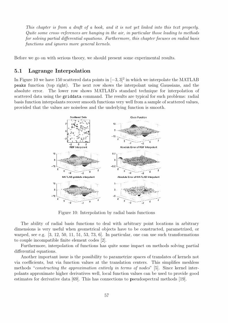
This chapter is from a draft of a book, and it is not yet linked into this text properly.Quite some cross–references are hanging in the air, in particular those leading to methodsfor solving partial differential equations. Furthermore, this chapter focuses on radial basisfunctions and ignores more general kernels.

Before we go on with serious theory, we should present some experimental results.

5.1 Lagrange Interpolation

In Figure 10 we have 150 scattered data points in [−3, 3]2 in which we interpolate the MATLABpeaks function (top right). The next row shows the interpolant using Gaussians, and theabsolute error. The lower row shows MATLAB’s standard technique for interpolation ofscattered data using the griddata command. The results are typical for such problems: radialbasis function interpolants recover smooth functions very well from a sample of scattered values,provided that the values are noiseless and the underlying function is smooth.

Figure 10: Interpolation by radial basis functions

The ability of radial basis functions to deal with arbitrary point locations in arbitrarydimensions is very useful when geometrical objects have to be constructed, parametrized, orwarped, see e.g. [3, 12, 50, 11, 51, 53, 73, 6]. In particular, one can use such transformationsto couple incompatible finite element codes [2].

Furthermore, interpolation of functions has quite some impact on methods solving partialdifferential equations.

Another important issue is the possibility to parametrize spaces of translates of kernels notvia coefficients, but via function values at the translation centers. This simplifies meshlessmethods “constructing the approximation entirely in terms of nodes” [5]. Since kernel inter-polants approximate higher derivatives well, local function values can be used to provide goodestimates for derivative data [69]. This has connections to pseudospectral methods [19].

57

5.2 Interpolation of Mixed Data

It is quite easy to allow much more general data for interpolation by radial basis functions.For example, consider recovery of a multivariate function f from data including the values∂f∂x2

(z),∫Ω f(t)dt. The basic trick, due to Z.M. Wu [75], is to use special trial functions

∂φ(‖x− z‖2)

∂x2for

∂f

∂x2(z)

∫

Ωφ(‖x− t‖2)dt for

∫

Ωf(t)dt

to cope with these requirements. In general, if a linear functional λ defines a data value λ(f)for a function f as in the above cases with λ1(f) = ∂f

∂x2(z), λ2(f) =

∫Ω f(t)dt, the special trial

function uλ(x) to be added is

uλ(x) := λtφ(‖x− t‖2) for λt(f(t))

where the upper index denotes the variable the functional acts on. If m = n functionalsλ1, . . . , λm are given, the span (2.9) of trial functions is to be replaced by

u(x) =n∑

k=1

akλtkφ(‖x− t‖2).

The interpolation system (2.11) turns into

λju =n∑

k=1

akλtkλ

xjφ(‖x− t‖2), 1 ≤ j ≤ n (5.1)

with a symmetric matrix composed of λtkλ

xjφ(‖x− t‖2), 1 ≤ j, k ≤ n which is positive definite

if the functionals are linearly independent and φ is positive definite.

−1

−0.5

0

0.5

1

−1

−0.5

0

0.5

1

−4

−3

−2

−1

0

1

2

3

4

x 104

Figure 11: Generalized interpolant to Neumann data

To give an example with general functionals, Figure 11 shows an interpolation to Neumanndata +1 and -1 on each half of the unit circle, respectively, in altogether 64 points by linearcombinations of properly scaled Gaussians.

58

In case of conditionally positive definite radial basis functions, the span of (4.21) or (4.24)turns into

u(x) :=n∑

k=1

akλtkφ(‖x− t‖2) +

q∑

ℓ=1

bℓpℓ(x)

while the additional condition (4.18) is replaced by

n∑

k=1

αkλtkpℓ(t) = 0, 1 ≤ ℓ ≤ q

and the interpolation problem is solvable, if the additional condition

λtkp(t) = 0 for all 1 ≤ k ≤ n and p ∈ P d

Q−1 implies p = 0

is imposed, replacing (4.18) and IP–unisolvency.Another example of recovery from non-Lagrange data is the construction of Lyapounov

basins from data consisting of orbital derivatives [24, 25].The flexibility to cope with general data is the key to various applications of radial ba-

sis functions within methods solving partial differential equations. Collocation techniques, astreated in books on numerical methods for solving partial differential equations, solve par-tial differential equations numerically by interpolation of values of differential operators andboundary conditions.

Another important aspect is the possibility to implement additional linear conditions orconstraints like

λ(u) :=∫

Ωu(x)dx = 1

on a trial function. For instance, this allows to handle conservation laws and is inevitablefor finite-volume methods. A constraint like the one above, when used as additionaldata, adds another degree of freedom to the trial space by addition of the basis functionuλ(x) := λtφ(‖x− t‖2), and at the same time it uses this additional degree of freedom to satisfythe constraint. This technique deserves much more attention in applications.

5.3 Error Behavior

If exact data come from smooth functions f , and if smooth kernels K or radial basis functionsφ are used for interpolation, users can expect very small interpolation errors. In particular,the error goes to zero when the data samples are getting dense. The actual error behavior islimited by the smoothness of both f and φ. Quantitative error bounds can be obtained fromthe standard literature [10, 71] and recent papers [48]. They are completely local, and they arein terms of the fill distance

h := h(X,Ω) := supy∈Ω

minx∈X

‖x− y‖2 (5.2)

of the discrete set X = x1, . . . , xn of centers with respect to the domain Ω where the erroris measured. The interpolation error converges to zero for h → 0 at a rate dictated by theminimum smoothness of f and φ. For infinitely smooth radial basis functions like the Gaussianor multiquadrics, convergence even is exponential [40, 76] like exp(−c/h). Derivatives arealso convergent as far as the smoothness of f and φ allows, but at a smaller rate, of course.

59

10−0.7

10−0.5

10−0.3

10−0.1

100.1

100.3

10−6

10−5

10−4

10−3

10−2

10−1

100

101

Gauss, scale=0.5Wendland C2, scale=50Thin−plate spline, scale=1

Inverse Multiquadric, scale=1Multiquadric, scale=0.8

Figure 12: Nonstationary interpolation to a smooth function as a function of fill distance

This is particularly important when applications require good reproductions of derivatives, e.g.velocity fields or stress tensors.

For interpolation of the smooth peaks function provided by MATLAB and used alreadyin Figure 10, the error behavior on [−3, 3]2 as a function of fill distance h is given by Figure12. It can be clearly seen that smooth φ yield smaller errors with higher convergence rates. Incontrast to this, Figure 13 shows interpolation to the nonsmooth function

f(x, y) = 0.03 ∗ max(0, 6 − x2 − y2)2, (5.3)

on [−3, 3]2, where now the convergence rate is dictated by the smoothness of f instead of φand is thus more or less fixed. Excessive smoothness of φ never spoils the error behavior, butinduces excessive instability, as we shall see later.

5.4 Stability

But there is a serious drawback when using radial basis functions on dense data sets, i.e. withsmall fill distance. The condition of the matrices used in (2.11) and (5.1) will get extremelylarge if the separation distance

S(X) :=1

2min

1≤i<j≤n‖xi − xj‖2

of points of X = x1, . . . , xn gets small. Figure 14 shows this effect in the situation of Figure12.

If points are distributed well, the separation distance S(X) will be proportional to thefill distance h(X,Ω) of (5.2). In fact, since the fill distance is the radius of the largest ballwith arbitrary center in the underlying domain Ω without any data point in its interior, theseparation distance S(X) is the radius of the smallest ball anywhere without any data pointin its interior, but with at least two points of X on the boundary. Thus for convex domains

60

10−0.7

10−0.5

10−0.3

10−0.1

100.1

100.3

10−3

10−2

10−1

100

101

Gauss, scale=0.5

Wendland C2, scale=50

Thin−plate spline, scale=1

Inverse Multiquadric, scale=1

Multiquadric, scale=0.8

Figure 13: Nonstationary interpolation to a nonsmooth function as a function of fill distance

one always has S(X) ≤ h(X,Ω). But since separation distance only depends on the closestpair of points and ignores the rest, it is reasonable to avoid unusually close points leading tosome S(X) which is considerably smaller than h(X,Ω). Consequently, a distribution of datalocations in X is called quasi–uniform if there is a positive uniformity constant γ ≤ 1 suchthat

γ h(X,Ω) ≤ S(X) ≤ h(X,Ω). (5.4)

To maintain quasi-uniformity, it suffices in most cases to delete “duplicates”. Furthermore,there are sophisticated “thinning” techniques [20, 17, 72] to keep fill and separation distanceproportional, i.e. to assure quasi-uniformity at multiple scaling levels.

5.5 Uncertainty Principle

Unless radial basis functions are rescaled in a data-dependent way, it can be proven [56]that there is a close link between error and stability, even if fill and separation distance areproportional. In fact, both are tied to the smoothness of φ, letting stability become worseand errors become smaller when taking smoother radial basis functions. This is kind of anUncertainty Principle:

It is impossible to construct radial basis functions which guarantee good stability andsmall errors at the same time.

We illustrate this by an example. Since [56] proves that the square of the L∞ error roughlybehaves like the smallest eigenvalue of the interpolation matrix, Figure 15 plots the product ofthe MATLAB condition estimate condest with the square of the L∞ error for the nonstationaryinterpolation of the MATLAB peaks function, used already for Figures 12, 6, and 14 to showthe error and condition behavior there. Note that the curves do not vary much if compared toFigure 14.

Thus smoothness of radial basis functions must be chosen with some care, and chosendependent on the smoothness of the function to be approximated. From the point of view of

61

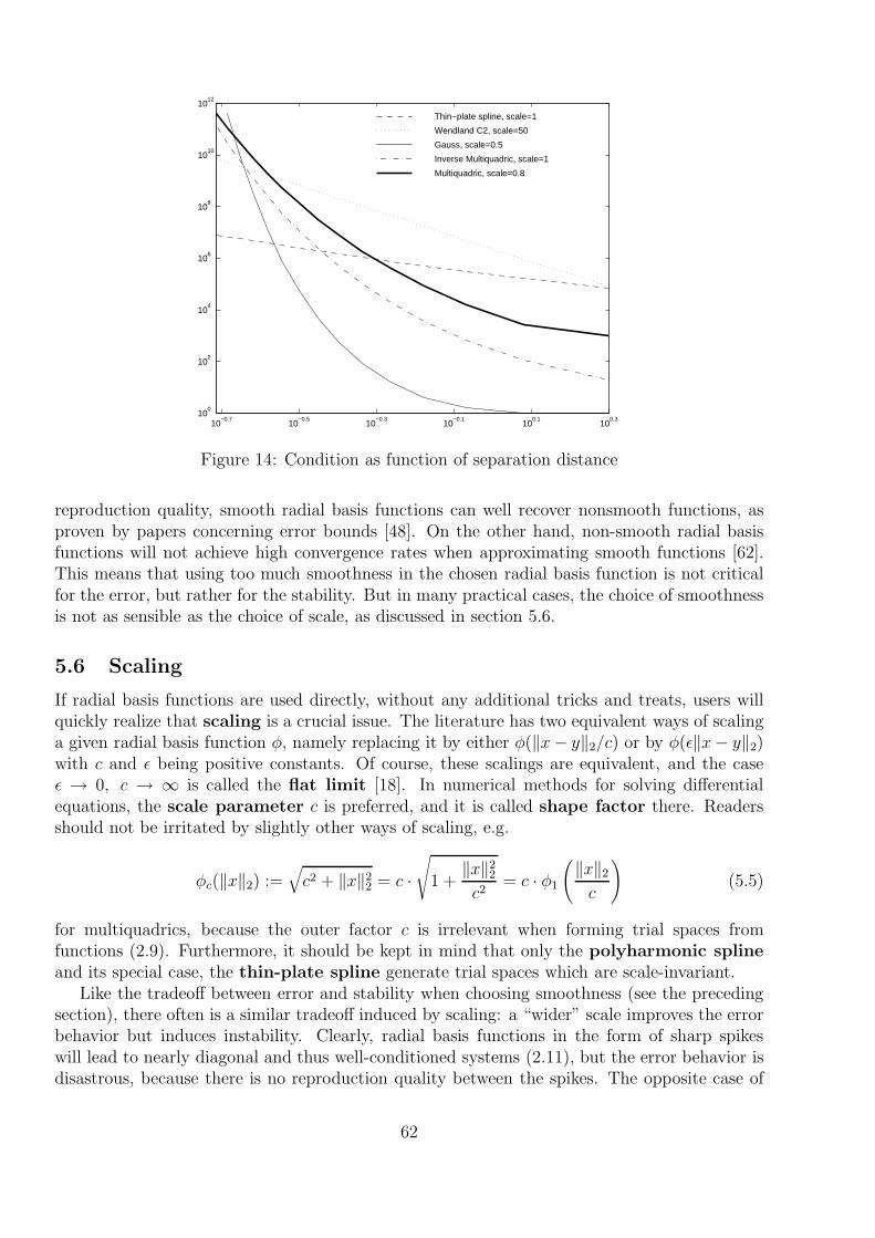
10−0.7

10−0.5

10−0.3

10−0.1

100.1

100.3

100

102

104

106

108

1010

1012

Gauss, scale=0.5




Multiquadric, scale=0.8

Figure 14: Condition as function of separation distance

reproduction quality, smooth radial basis functions can well recover nonsmooth functions, asproven by papers concerning error bounds [48]. On the other hand, non-smooth radial basisfunctions will not achieve high convergence rates when approximating smooth functions [62].This means that using too much smoothness in the chosen radial basis function is not criticalfor the error, but rather for the stability. But in many practical cases, the choice of smoothnessis not as sensible as the choice of scale, as discussed in section 5.6.

5.6 Scaling

If radial basis functions are used directly, without any additional tricks and treats, users willquickly realize that scaling is a crucial issue. The literature has two equivalent ways of scalinga given radial basis function φ, namely replacing it by either φ(‖x− y‖2/c) or by φ(ǫ‖x− y‖2)with c and ǫ being positive constants. Of course, these scalings are equivalent, and the caseǫ → 0, c → ∞ is called the flat limit [18]. In numerical methods for solving differentialequations, the scale parameter c is preferred, and it is called shape factor there. Readersshould not be irritated by slightly other ways of scaling, e.g.

φc(‖x‖2) :=√c2 + ‖x‖2

2 = c ·√

1 +‖x‖2

2

c2= c · φ1

(‖x‖2

c

)(5.5)

for multiquadrics, because the outer factor c is irrelevant when forming trial spaces fromfunctions (2.9). Furthermore, it should be kept in mind that only the polyharmonic splineand its special case, the thin-plate spline generate trial spaces which are scale-invariant.

Like the tradeoff between error and stability when choosing smoothness (see the precedingsection), there often is a similar tradeoff induced by scaling: a “wider” scale improves the errorbehavior but induces instability. Clearly, radial basis functions in the form of sharp spikeswill lead to nearly diagonal and thus well-conditioned systems (2.11), but the error behavior isdisastrous, because there is no reproduction quality between the spikes. The opposite case of

62

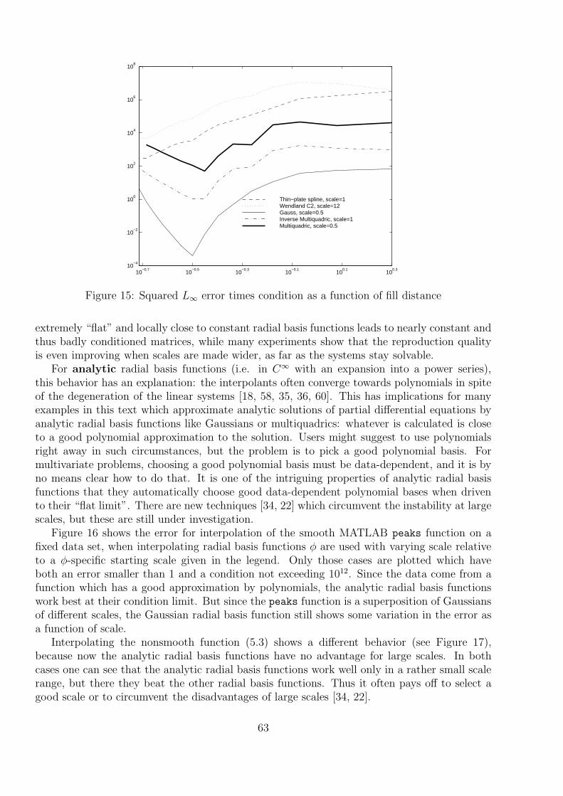
10−0.7

10−0.5

10−0.3

10−0.1

100.1

100.3

10−4

10−2

100

102

104

106

108

Gauss, scale=0.5Wendland C2, scale=12Thin−plate spline, scale=1

Inverse Multiquadric, scale=1Multiquadric, scale=0.5

Figure 15: Squared L∞ error times condition as a function of fill distance

extremely “flat” and locally close to constant radial basis functions leads to nearly constant andthus badly conditioned matrices, while many experiments show that the reproduction qualityis even improving when scales are made wider, as far as the systems stay solvable.

For analytic radial basis functions (i.e. in C∞ with an expansion into a power series),this behavior has an explanation: the interpolants often converge towards polynomials in spiteof the degeneration of the linear systems [18, 58, 35, 36, 60]. This has implications for manyexamples in this text which approximate analytic solutions of partial differential equations byanalytic radial basis functions like Gaussians or multiquadrics: whatever is calculated is closeto a good polynomial approximation to the solution. Users might suggest to use polynomialsright away in such circumstances, but the problem is to pick a good polynomial basis. Formultivariate problems, choosing a good polynomial basis must be data-dependent, and it is byno means clear how to do that. It is one of the intriguing properties of analytic radial basisfunctions that they automatically choose good data-dependent polynomial bases when drivento their “flat limit”. There are new techniques [34, 22] which circumvent the instability at largescales, but these are still under investigation.

Figure 16 shows the error for interpolation of the smooth MATLAB peaks function on afixed data set, when interpolating radial basis functions φ are used with varying scale relativeto a φ-specific starting scale given in the legend. Only those cases are plotted which haveboth an error smaller than 1 and a condition not exceeding 1012. Since the data come from afunction which has a good approximation by polynomials, the analytic radial basis functionswork best at their condition limit. But since the peaks function is a superposition of Gaussiansof different scales, the Gaussian radial basis function still shows some variation in the error asa function of scale.

Interpolating the nonsmooth function (5.3) shows a different behavior (see Figure 17),because now the analytic radial basis functions have no advantage for large scales. In bothcases one can see that the analytic radial basis functions work well only in a rather small scalerange, but there they beat the other radial basis functions. Thus it often pays off to select agood scale or to circumvent the disadvantages of large scales [34, 22].

63

10−1

100

101

102

10−3

10−2

10−1

100

Gauss, scale=1




Multiquadric, scale=1

Figure 16: Error as function of relative scale, smooth case

Like in finite element methods, users might want to scale the basis functions in a data-dependent way, making the scale c in the sense of using φ(‖x − y‖2/c) proportional to thefill distance h as in (5.2). This is often called a stationary setting, e.g. in the context ofwavelets and quasi-interpolation. If the scale is fixed, the setting is called nonstationary,and this is what we were considering up to this point. Users must be aware that the errorand stability analysis, as described in the previous sections, apply to the nonstationary case,while the stationary case will not converge for h→ 0 in case of unconditionally positive definiteradial basis functions [8, 9]. But there is a way out: users can influence the “relative” scaleof c with respect to h in order to achieve a good compromise between error and stability.The positive effect of this can easily be observed [57], and for special situations there is asound theoretical analysis called approximate approximation [41]. Figure 18 shows thestationary error behavior for interpolation of the smooth MATLAB peaks function when usingdifferent radial basis functions φ at different starting scales. It can be clearly seen how the errorgoes down to a certain small level depending on the smoothness of φ, and then stays roughlyconstant. Using larger starting radii decreases these saturation levels, as Figure 19 shows.

Due to the importance of relative scaling, users are strongly advised to always run theirprograms with an adjustable scale of the underlying radial basis functions. Experimenting withsmall systems at different scales give a feeling of what happens, and users can fix the relativescale of c versus h rather cheaply. Final runs on large data can then use this relative scaling. Inmany cases, given problems show a certain “intrinsic” preference for a certain scale, as shownin Figure 17, but this is an experimental observation which still is without proper theoreticalexplanation.

5.7 Practical Rules

If users adjust the smoothness and the scaling of the underlying radial basis function along thelines of the previous sections, chances are good to get away with relatively small and sufficientlystable systems. The rest of the text contains plenty of examples for this observation.

64

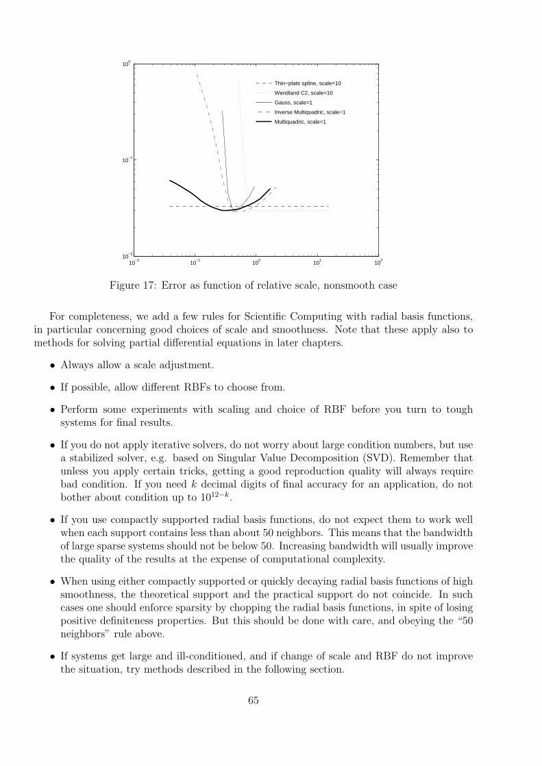
10−2

10−1

100

101

102

10−2

10−1

100

Gauss, scale=1




Multiquadric, scale=1

Figure 17: Error as function of relative scale, nonsmooth case

For completeness, we add a few rules for Scientific Computing with radial basis functions,in particular concerning good choices of scale and smoothness. Note that these apply also tomethods for solving partial differential equations in later chapters.

• Always allow a scale adjustment.

• If possible, allow different RBFs to choose from.

• Perform some experiments with scaling and choice of RBF before you turn to toughsystems for final results.

• If you do not apply iterative solvers, do not worry about large condition numbers, but usea stabilized solver, e.g. based on Singular Value Decomposition (SVD). Remember thatunless you apply certain tricks, getting a good reproduction quality will always requirebad condition. If you need k decimal digits of final accuracy for an application, do notbother about condition up to 1012−k.

• If you use compactly supported radial basis functions, do not expect them to work wellwhen each support contains less than about 50 neighbors. This means that the bandwidthof large sparse systems should not be below 50. Increasing bandwidth will usually improvethe quality of the results at the expense of computational complexity.

• When using either compactly supported or quickly decaying radial basis functions of highsmoothness, the theoretical support and the practical support do not coincide. In suchcases one should enforce sparsity by chopping the radial basis functions, in spite of losingpositive definiteness properties. But this should be done with care, and obeying the “50neighbors” rule above.

• If systems get large and ill-conditioned, and if change of scale and RBF do not improvethe situation, try methods described in the following section.

65

10−0.6

10−0.4

10−0.2

100

100.2

10−9

10−8

10−7

10−6

10−5

10−4

10−3

10−2

10−1

100

101

Gauss, start scale=8

Wendland C2, start scale=100

Thin−plate spline, start scale=1

Inverse Multiquadric, start scale=20

Multiquadric, start scale=15

Figure 18: Stationary interpolation to a smooth function at small starting scales

• Use blockwise iteration (“domain decomposition”) first, because it is simple and oftenrather efficient.

• Blockwise iteration can be speeded up by precalculation of LR decompositions of blocks.

• If all of this does not work, try partitions of unity, multilevel methods, or special precon-ditioning techniques. You are now at current research level, and you should look into thenext section.

5.8 Sensitivity to Noise

So far, the discussion focused on noiseless data, with the exception of Figure 7. If users expectnoise in the data, an interpolatory recovery is not appropriate, because it treats noise as data.In most of the later sections of this text, data are right-hand sides or boundary values for partialdifferential equations, and they usually are given as noiseless functions which can be evaluatedanywhere. Thus the rest of the text does not treat noisy inputs in detail. But at this point,some remarks are appropriate.

In all noisy situations, interpolation should be replaced by approximation. This can be donein various ways leading to stabilization.

A primitive, but often quite sufficient technique is to run a smoothing process on the rawdata and to recover the unknown function from the smoothed data instead of the raw data.

Another standard trick is to solve (2.11) in the L2 sense with oversampling, if only n << mtrial points xj are used for m data points yk. The trial points can then be placed rather freelywith a large separation distance, while a small separation distance of data points will not have adramatic effect on stability any more. However, there is not very much theoretical and practicalwork done on unsymmetric recovery techniques [59, 61, 60].

A third possibility is the old Levenberg-Marquardt trick of adding a positive value λ intothe diagonal of the kernel matrix of (2.11) with entries φ(‖xj − xk‖2). As is well-known from

66

10−0.7

10−0.5

10−0.3

10−0.1

100.1

100.3

10−7

10−6

10−5

10−4

10−3

10−2

10−1

100

101

Gauss, start scale=6Wendland C2, start scale=50Thin−plate spline, start scale=5

Inverse Multiquadric, start scale=15Multiquadric, start scale=10

Figure 19: Stationary interpolation to a smooth function at wider starting scales

literature on spline smoothing, this leads to an approximant achieving a tradeoff betweensmoothness and reproduction quality which can be controlled by λ. If a stochastic backgroundis available, there are methods to estimate λ properly, e.g. by cross-validation. However,in most cases users adjust λ experimentally. This technique also helps to fight instabilitywhen working on irregularly distributed data [72], because it is able to shift the stability fromdependence on the separation distance to dependence on the fill distance (see section 5.4).

A fourth possibility is regularization, for example using a singular-value decomposition asdescribed in section 3.4.

In general, one can replace the system (2.11) by an optimization method which penalizesthe reproduction error on one hand and either a complexity or smoothness criterion on theother, allowing a fair amount of control over the tradeoff between error and stability. Penaltiesfor the discrete reproduction error can be made in various discrete norms, the ℓ1 and ℓ∞ casehaving the advantage to lead to linear optimization restrictions, while the discrete ℓ2 normleads to quadratic ones. For radial basis functions of the form (2.9) or (4.21), the quadraticform

‖u‖2φ :=

n∑

j,k=1

αjαkφ(‖xj − xk‖2) (5.6)

is a natural candidate for penalizing high derivatives without evaluating any. This is due tothe standard fact that the above expression is a squared norm in a native space of functionswith about half the smoothness of φ, penalizing all available derivatives there. For details,we have to refer to basic literature [10, 71] on the theory of radial basis functions. But eventhough we skip over native spaces here, all users should be aware that they always lure inthe theoretical background, and that all methods based on radial basis functions implicitlyminimize the above quadratic form under all functions in the native space having the samedata. This has a strong regularization effect which is the background reason why radialbasis function or more general kernel methods work well for many ill-posed and inverseproblems [31, 37, 67, 14, 13, 32, 33, 38, 55, 49]. The above strategy of minimizing the quadraticform (5.6) also is central for modern methods of machine learning, but we cannot pursue

67

this subject in detail here [15, 65, 66].

0 20 40 60 80 100 120 140 160 180 2000

0.1

0.2

0.3

0.4

0.5

0.6

0.7

0.8

0.9

1

Points

Eps

ilon

no noise2 % noise

Figure 20: Connection between ǫ and the number n(ǫ) of necessary points

Let us use minimization of the quadratic form (5.6) to provide an example for the tradeoffbetween error and complexity. Again, the basic situation is interpolation to the MATLABpeaks function, this time in 14×14=196 regularly distributed points in [−3, 3]2 by Gaussians ofscale 1. The global L∞[−3, 3]2 error of the exact interpolation on these data is 0.024, evaluatedon a fine grid with 121×121=14641 points. But now we minimize the quadratic form (5.6)under the constraints

−ǫ ≤n∑

j=1

αjφ(‖xj − xk‖2) − f(xk) ≤ ǫ, 1 ≤ k ≤ n (5.7)

for positive ǫ. The case of ǫ = 0 is exact interpolation using all 196 data points and trialfunctions. For positive ǫ, the usual Karush-Kuhn-Tucker conditions imply that only thosepoints xk are actually used where one of the bounds in (5.7) is attained with equality. Thenumber n(ǫ) of required points grows up to the maximally possible n(0) = 196 when ǫ decreases.Figure 20 shows this for the case of exact and noisy data.

But even more interesting is the behavior of the global L∞[−3, 3]2 error E(ǫ) as a functionof ǫ. Figure 21 shows that E(ǫ) roughly follows the behavior of ǫ when plotted as a function ofthe required points n(ǫ). Both curves are experimentally available, and one can read off thatthe optimal choice of ǫ in the noisy case is at the point where the curve takes its L-turn, i.e. atthe point of largest curvature around n = 40. This can be viewed as an experimental methodto determine the noise level. Note that it does not pay off to use more points, and note thesimilarity to the L-curve technique [30].

But also for exact data, these curves are useful. Since the maximum value of the peaks

function is about 8.17, one can get a relative global accuracy of 1% using roughly 60 points forexact data. It makes no sense to use the full 196 points, even for exact data, if exact resultsare not required. Of course, larger noise levels lead to smaller numbers of required points,but a thorough investigation of these tradeoff effects between error and complexity is still achallenging research topic.

68

0 20 40 60 80 100 120 140 160 180 2000

0.5

1

1.5

Points

Glo

bal e

rror

no noise2 % noise

Figure 21: Error E(ǫ) as a function of the number n(ǫ) of necessary points

.... incomplete...

Demos on power functions and on point selection

.... incomplete...

6 Error Analysis

This section is the core for any error analysis of interpolation or approximation methods. Thereare essentially two possible approaches:

1. via upper bounds on the power function and

2. via “sampling inequalities”.

These share some common tools. e.g. the concept of “norming sets” and local polynomialapproximation. The second alternative is more modern, and thus I chose it. But, as the otherone, it is hardcore mathematics and it would take too much time to present a complete rigidproof including all the details. Thus I shall focus on motivating and explaining the importantingredients, but I shall skip over tedious and detailed calculations. In order to start with aneasy case, we shall focus on univariate sampling inequalities first.

6.1 Sampling Inequalities

The basic idea of sampling inequalities is the following.

Assume that a function s approximates or interpolates a function f on a discrete subset X ofits domain Ω. Then f − s is small or even zero on X. How large can the error function f − s

69

be outside of X? If, for instance, any directional derivative of both f and s is bounded aboveby some constant K, we can write

|f(x) − s(x)| ≤ |f(xj) − s(xj)| + 2K · ‖x− xj‖2

if the line connecting x and xj ∈ X is in Ω and if we integrate the directional derivative alongthe line. If we define the fill distance

h := h(X,Ω) := supx∈Ω

minxj∈X

‖x− xj‖2

of X in Ω and if Ω is convex, this yields the simple error bound

‖f − s‖∞,Ω ≤ 2K · h,

but we need to have K under control, i.e. in terms of some tricky high–order norm ‖f‖ of f .

Here is a more general description of the above argument, applied to the error function:

If a smooth function has a bound on its highest derivatives, and if it is small on a largeset of points which “fills” the domain, then it should be small everywhere.

We can apply such a result nicely in our kernel–based methods, because if we have a functionf in the native space N , we know that its interpolant sf,X on a set X minimizes the nativespace (semi–) norm under all other interpolants, and thus |sf,X |N ≤ |f |N will hold in the nativespace (semi–) norm. Thus we should be able to infer that f − sf,X is small if the fill distanceh of X is small, i.e. we want something like

‖f − sf,X‖∞,Ω ≤ F (h(X,Ω))|f |N (6.1)

with F (h) → 0 for h → 0. This works along the lines of Theorem (3.10) and Corollary (4.33)if we can bound the power function by F (h(X,Ω)). For about two decades, this technique wasthe standard way of obtaining error bounds for kernel–based interpolants.

However, a more general bound like

‖f‖∞,Ω ≤ F (h(X,Ω))|f |N + C · ‖f‖∞,X (6.2)

holding for all f in the native space N would imply (6.1) with a slightly larger constant, if itis applied to f − sf,X via

‖f − sf,X‖∞,Ω ≤ F (h(X,Ω))|f − sf,X |N + C · ‖f − sf,X‖∞,X

≤ F (h(X,Ω))|f − sf,X |N≤ F (h(X,Ω))(|f |N + |sf,X |N )≤ 2F (h(X,Ω))|f |N .

We shall thus go for (6.2) directly, but we shall allow other norms than the ∞–norms, and weshall consider general spaces instead of native spaces for kernels.

Note that (6.2) is of crucial importance for all kinds of discretization processes. If a function fis discretized by taking values in X, users must often know that it does not get large betweenthe data sites. This is exactly provided by (6.2) in case of F (h) → 0 for h→ 0.

70

6.2 Univariate Case

Since the forthcoming mathematical analysis is quite hard, let us first start with the muchsimpler univariate case. We shall work on a bounded interval I := [a, b] ⊂ IR, and there weshall define the (semi–) inner products and (semi–) norms

(f, g)j :=∫

If (j)(t)g(j)(t)dt for all f, g ∈ Cj(I)

|f |∞,X := supt∈X

|f(t)| for all f ∈ C(I), X ⊂ I,

|f |22,X := h(X,Ω)∑

x∈X

f 2(x) for all f ∈ C(I), X ⊂ I, |X| <∞.

Throughout, we shall confine ourselves to subsets X ⊂ [a, b] with fill distance h = h(X, [a, b]).

Lemma 6.3 Given g ∈ C1(I) and a subset X of [a, b] with fill distance h. Then we have

‖g‖0 ≤ h |g|1 +√

2|g|2,X,

‖g‖0 ≤ h |g|1 +√

2(b− a)|g|∞,X,

‖g‖∞,I ≤ h ‖g′‖∞,I +|g|∞,X,

‖ g‖∞,I ≤√h |g|1 +|g|∞,X.

(6.4)

Proof: For all x ∈ I we can take its closest neighbor xj ∈ X with distance |x− xj | ≤ h. Then

g(x) = g(xj) +∫ x

xj

g′(τ)dτ

|g(x)| ≤ |g(xj)| +∫ x

xj

|g′(τ)|dτ‖g‖∞,I ≤ h ‖g′‖∞,I + |g|∞,X

for all x ∈ I. With the Cauchy–Schwarz inequality we we get

|g(x)| ≤ |g(xj)| +∣∣∣∣∣

∫ x

xj

12dτ

∣∣∣∣∣

1/2

·∣∣∣∣∣

∫ x

xj

(g′(τ))2dτ

∣∣∣∣∣

1/2

(x ∈ I)

≤ |g(xj)| + |x− xj|1/2 ·∣∣∣∣∣

∫ x

xj

(g′(τ))2dτ

∣∣∣∣∣

1/2

,

‖ g‖∞,I ≤√h |g|1 + |g|∞,X.

By taking squares and the usual trick

(a+ b)2 ≤ a2 + b2 + 2|ab| ≤ 2a2 + 2b2

we see thatg(x)2 ≤ 2g(xj)

2 + 2|x− xj | ·∫ x

xj

(g′(τ))2dτ

and by integration we find

∫ xxjg(t)2dt ≤ 2|x− xj |g(xj)

2 +∫ x

xj

2|t− xj | ·∫ t

xj

(g′(τ))2dτdt

= 2|x− xj |g(xj)2 +

∫ x

xj

(g′(τ))2∫ τ

x2|t− xj |dtdτ

≤ 2|x− xj |g(xj)2 + |x− xj |2 ·

∫ x

xj

(g′(τ))2dτ.

71

From here on we superimpose different integrals of this form to a full integral over [a, b] to endup with

‖g‖20 ≤ h2 |g|21 + 2(b− a)|g|2∞,X

‖g‖0 ≤ h |g|1 +√

2(b− a)|g|∞,X

where we used√a2 + b2 ≤ a + b for a, b > 0. If we sum up the discrete values, we arrive at

‖g‖20 ≤ h2 |g|21 + 2h

N∑

j=1

g(xj)2

‖g‖0 ≤ h |g|1 +√

2|g|2,X.

2

6.3 Example: Univariate Splines

In the notation of the text on splines, we have

Theorem 6.5 Let f ∈ Ck[a, b] be interpolated by s∗ in N ≥ k data with a fill distance

h := supx∈[a,b]

minxj

|x− xj |.

Then there is a constant ck depending only on k and [a, b], but not on f or the data or h, suchthat

‖f − s∗‖L2[a,b] ≤ ckhk|f − s∗|k ≤ 2ckh

k|f |k,‖f − s∗‖L∞[a,b] ≤ ckh

k−1/2|f − s∗|k ≤ 2ckhk−1/2|f |k.

Proof: Note that the zeros of f − s∗ have a distance of at most 2h between each other and ofat most h ≤ 2h to the boundary. By Rolle’s theorem, there are zeros of (f − s∗)′ with distanceof at most 4h between each other and 3h to the boundary. This means that we can use the filldistance 4h for the zeros of the first derivative. This works up to the derivative of order k − 1,which has zeros with distance of at most 4k−1h between each other and to the boundary. Usinginduction on the previous Lemma yields

‖f − s∗‖L2[a,b] ≤ h · 4h · · · 4k−1h|f − s∗|k =: ckhk|f − s∗|k

and the left–hand parts of the assertions follow.

For the right-hand parts we use the optimality condition |s∗|k ≤ |f |k. 2

If some additional boundary conditions are satisfied, the convergence order doubles.

Theorem 6.6 If, in addition, f ∈ C2k[a, b] and if (f − s∗)(j) vanishes at a and b for j =0, . . . , k − 1, then

‖f − s∗‖L2[a,b] ≤ c2kh2k|f |2k.

‖f − s∗‖L∞[a,b] ≤ c2kh2k−1|f |2k.

Proof: We can use the orthogonality relation

(f − s∗, s∗)k = 0

72

and do integration by parts via

|f − s∗|2k = (f − s∗, f − s∗)k

= (f − s∗, f)k

=∫ b

a(f − s∗)(k)(t)f (k)(t)dt

= (−1)k∫ b

a(f − s∗)(0)(t)f (2k)(t)dt

≤ ‖f − s∗‖L2[a,b]|f |2k.

Then‖f − s∗‖2

L2[a,b] ≤ c2kh2k|f − s∗|2k

≤ c2kh2k‖f − s∗‖L2[a,b]|f |2k

‖f − s∗‖L2[a,b] ≤ c2kh2k|f |2k.

Similarly,‖f − s∗‖2

L∞[a,b] ≤ c2kh2k−1|f − s∗|2k

≤ c2kh2k−1‖f − s∗‖L2[a,b]|f |2k

≤√b− ac2kh

2k−1‖f − s∗‖L∞[a,b]|f |2k

‖f − s∗‖L∞[a,b] ≤ c2kh2k−1|f |2k.

Note that the above argument used Rolle’s theorem, which does not hold in multivariatesettings. Thus we cannot generalize this approach directly to functions of several variables.

6.4 Univariate Polynomial Reproduction

Our goal is to prove a multivariate version of a sampling inequality. But already in the univariatecase, a general inequality like

‖u‖∞,[a,b] ≤ C(hk−1/2|u|k + |u|∞,X

)

means that for all polynomials p ∈ IP k we have

‖p‖∞,[a,b] ≤ C|p|∞,X. (6.7)

Then X must be unisolvent, but this is not enough. If we take X to contain exactly k points,an equality of the above form cannot hold. To see this, fix k − 1 zeros and prescribe 1 at apoint which moves close to a zero. The resulting Lagrange basis polynomial will converge toinfinity except at the zeros.

But if we take many more than k points, i.e. we do some oversampling, chances are betterto get something like (6.7). If we extend (6.7) trivially to the right, we get

‖p‖∞,[a,b] ≤ C|p|∞,X ≤ C‖p‖∞,[a,b]

and see that X must guarantee norm equivalence of a discrete norm with a “continuous” norm.We could call X a “norming set”, but there is a more general definition of that notion, and weprovide it later.

To move closer to (6.7), let us fix a polynomial p ∈ IP k with ‖p‖∞,[a,b] = 1. We need to showthat such a polynomial cannot be too small on a nontrivial set X, but we want to get awaywith a smallest possible set X. For simplicity, we take a t ∈ [a, b] with |p(t)| = 1 and ask: Howfar must we go to let |p| drop below 1/2? Fortunately, we have a bound on the derivative:

73

Theorem 6.8 Any univariate polynomial of degree n satisfies Markov’s inequality

‖p′‖∞,[−1,1] ≤ n2‖p‖∞,[−1,1].

We skip over the proof, but by norm equivalence there must be an n–dependent constant thatdoes the job. The only problem is to prove that the constant is n2.

Now we know that our special polynomial has a derivative ‖p′‖∞,[−1,1] ≤ n2 if we assume thatthe interval is [−1, 1]. Thus, in order to let p go down to 1/2 we need to go at least a distance1/2n2. If we know that X has a fill distance

h ≤ 1

2n2

we can be sure that we cannot reach a point with absolute value of p smaller than 1/2 whenstarting from t. This means that

|p|∞,X ≥ 1

2

and consequently ‖p‖∞,[−1,1] ≤ 2|p|∞,X. Thus we have

Theorem 6.9 If X ⊂ [−1, 1] is a set of fill distance h ≤ 12n2 , then

‖p‖∞,[−1,1] ≤ 2|p|∞,X

for all polynomials of degree at most n. 2

From now on we assume that the hypothesis of Theorem 6.9 is satisfied. Then X clearly isunisolvent, and we know that we can reproduce all polynomials p ∈ IP n by a nonunique formulalike

p(x) =∑

xj∈X

uj(x)p(xj). (6.10)

In our old notation, this is an under-determined linear system

PX · u(x) = p(x)

and one can impose additional conditions. In fact, there are efficient numerical techniques (e.g.moving least squares which produce useful admissible solutions.

Theorem 6.11 Under all possibilities to satisfy (6.10) under the conditions of Theorem 6.9there is one which has a uniformly bounded Lebesgue function

∑

xj∈X

|uj(x)| ≤ 2 for all x ∈ [−1, 1].

Proof: This statement is not at all evident, and for now we have to do an abstract existenceproof. We define the sampling operator

TX : f 7→ (f(x1), . . . , f(xN))T ∈ IRN ,

which is continuous on C[−1, 1] with the ‖.‖∞ norm and invertible on T (IP n) ⊂ IRN . It has abounded inverse

S : T (IP n) → IP n ⊂ C[−1, 1].

74

For each vector y ∈ T (IP n) ⊂ IRN there is a unique p ∈ IP n with such y = (p(x1), . . . , p(xN))T ,and thus for each x ∈ [−1, 1] we have a linear functional

λx : y = (p(x1), . . . , p(xN ))T 7→ p(x)

on T (IP n). By the Hahn–Banach theorem it has a norm–preserving extension to all ofIRN , and this is the abstract and non-constructive part of the argument. As a functional on allof IRN it can be written as

λx(y) :=N∑

j=1

uj(x)yj

with certain real values uj(x), and its norm must be

‖λx‖1 :=∑

xj∈X

|uj(x)| = supy∈IRN\0

∣∣∣∑

xj∈X uj(x)yj

∣∣∣

‖y‖∞

because the dual of IRN under the ‖.‖∞ norm is IRN with the L1 norm. But since the extensionis norm–preserving, this norm is equal to the norm of the functional on the subspace T (IP n).There it has the form λx = δx S, and thus

‖λx‖1 ≤ ‖δx‖ · ‖S‖

with operator norms

‖δx‖ = supf∈C[−1,1]\0

|f(x)

‖f‖∞≤ 1

and

‖S‖ := supT (p)∈T (IP n)\0

|p(x)|‖T (p)‖∞

≤ 2.

Thus we get the assertion. 2

It is an easy task to find functions uj(x) for which the Lebesgue function is pointwise minimal,while a certain polynomial reproduction of a degree n is required. It boils down to an L1

optimization problem, because we can write each uj(x) as uj(x) = aj − bj with nonnegativevariables to arrive at the linear optimization problem

Minimize 1TN(a + b) under PX(a− b) = p(x)

in normal form with nonnegative variables a, b ∈ IRN . This can be solved pointwise, but thesolution is rather strange, see figures 23 and 22. The theory of linear optimization implies thatat a certain point x there can be at most 2(n + 1) nonzero uj(x), but the functions uj are notlocalized around xj, as Figure 24 shows.

Thus it is an additional problem to find a stable solution which is localized in the sense thatuj(x) vanishes if x is “far” from xj . But this can be done by localizing the above argument.However, we shall not do this at this point. Instead, we start with the general multivariate caseand care for both localization and a bounded Lebesgue function.

75

−1 −0.8 −0.6 −0.4 −0.2 0 0.2 0.4 0.6 0.8 11

1.005

1.01

1.015

1.02

1.025

Figure 22: Minimal Lebesgue function for 17 equidistant points in [−1, 1] and polynomial degreen = 3

6.5 Norming Sets

As a little digression, we generalize the above construction, following an idea of Jetter, Stockler,and Ward.

... incomplete here.....

6.6 Multivariate Polynomial Reproduction

In the multivariate setting, we should go for sampling inequalities of the form

‖u‖W m2 (Ω) ≤ C

(hM−m|u|W M

2 (Ω) + h−m‖u‖∞,Xh

)

‖Dαu‖L∞(Ω) ≤ C(hM−|α|−d/2|u|W M

2 (Ω) + h−m‖u‖∞,Xh

) (6.12)

for all functions in the Sobolev space WM2 (Ω) with the inner product

(f, g)W M2 (Ω) :=

M∑

j=0

(f, g)j

(f, g)j :=∑

|α|=j

∫

ΩDαfDαg

and (semi–)norms‖f‖2

W M2 (Ω)

:= (f, f)W M2 (Ω)

|f |2W M

2 (Ω):= (f, f)M =

∑

|α|=j

∫

Ω|Dαf |2

where we use standard multivariate notation. If u is a polynomial of order at most M , then|u|2W M(Ω) = |u|M = 0 and our equations take a special form

‖p‖L2(Ω) ≤ C‖p‖∞,Xh

‖p‖L∞(Ω) ≤ C‖p‖∞,Xh

76

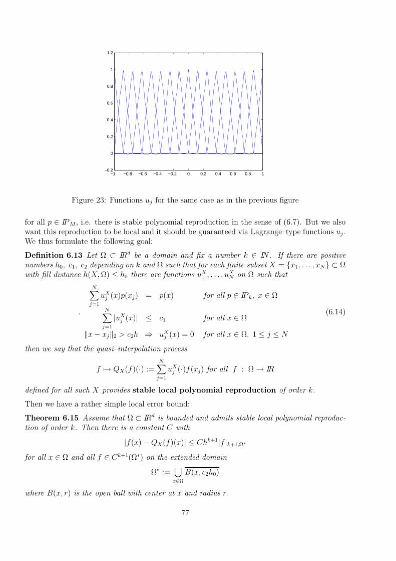
−1 −0.8 −0.6 −0.4 −0.2 0 0.2 0.4 0.6 0.8 1−0.2

0

0.2

0.4

0.6

0.8

1

1.2

Figure 23: Functions uj for the same case as in the previous figure

for all p ∈ IPM , i.e. there is stable polynomial reproduction in the sense of (6.7). But we alsowant this reproduction to be local and it should be guaranteed via Lagrange–type functions uj.We thus formulate the following goal:

Definition 6.13 Let Ω ⊂ IRd be a domain and fix a number k ∈ IN . If there are positivenumbers h0, c1, c2 depending on k and Ω such that for each finite subset X = x1, . . . , xN ⊂ Ωwith fill distance h(X,Ω) ≤ h0 there are functions uX

1 , . . . , uXN on Ω such that

.

N∑

j=1

uXj (x)p(xj) = p(x) for all p ∈ IP k, x ∈ Ω

N∑

j=1

|uXj (x)| ≤ c1 for all x ∈ Ω

‖x− xj‖2 > c2h ⇒ uXj (x) = 0 for all x ∈ Ω, 1 ≤ j ≤ N

(6.14)

then we say that the quasi–interpolation process

f 7→ QX(f)(·) :=N∑

j=1

uXj (·)f(xj) for all f : Ω → IR

defined for all such X provides stable local polynomial reproduction of order k.

Then we have a rather simple local error bound:

Theorem 6.15 Assume that Ω ⊂ IRd is bounded and admits stable local polynomial reproduc-tion of order k. Then there is a constant C with

|f(x) −QX(f)(x)| ≤ Chk+1|f |k+1,Ω∗

for all x ∈ Ω and all f ∈ Ck+1(Ω∗) on the extended domain

Ω∗ :=⋃

x∈Ω

B(x, c2h0)

where B(x, r) is the open ball with center at x and radius r.

77

−1 −0.8 −0.6 −0.4 −0.2 0 0.2 0.4 0.6 0.8 1−2

0

2

4

6

8

10

Figure 24: Derivative of u1 for the same case as in the previous figure

Proof: See Wendland’s book [71], p. 25/26. The basic trick is to introduce the local Taylorexpansion at x which has the same error bound and is reproduced by the quasi–interpolant.Then use the boundedness of the Lebesgue function to show that the error of the local Taylorexpansion carries over to the quasi–interpolant. 2.

Inspection of the proof shows that the extended domain is not necessary for all forms of localbounds.

To proceed towards an existence proof of stable local polynomial reproduction on nondegeneratedomains, we repeat our argument from the univariate case, but we can focus on k > 1 becausestable polynomial reproduction by constants is trivial, using the nearest neighbor of X to eachx ∈ Ω. Another choice for stable local approximation of order one is Shepard approximation,which we shall describe in the next section.

It does not suffice to use IP k–unisolvent subsets, because they will not have bounded Lebesguefunctions. We thus first aim at a proof of an inequality like

‖p‖∞,Ω ≤ c2‖p‖∞,X for all p ∈ IP k

for suitable domains Ω and finite sets X ⊂ Ω . We start with a polynomial p ∈ IP k withp(x) = ‖p‖∞,Ω = 1 and see how fast it can go down when moving away from x. On a ray goingfrom x to some other point z, the polynomial

q(t) := p (x+ t(z − x)), t ∈ [0, 1]

is univariate and of order at most k. We have

|p (x+ t(z − x)) − p(x)| = |q(t) − q(0)| =∣∣∣∣∫ t

0q′(t)dt

∣∣∣∣ ≤ t‖q′‖∞,[−1,1]

and use Markov’s inequality to get

|p (x+ t(z − x)) − p(x)| ≤ t(k − 1)2‖q‖∞,[−1,1] ≤ t(k − 1)2‖p‖∞,Ω

78

for all t ∈ [0, 1]. But for our choice of 1 = p(x) = ‖p‖∞,Ω we get

p

x+ t(z − x)︸︷︷︸

=:yt

= q(t) ≥ 1 − 2t(k − 1)2

leading to p(yt) ≥ 1/2 for all yt on the ray with t = ‖x − yt‖2 ≤ 14(k−1)2

. For all finite sets Xwith

minz∈X

‖x− z‖2 ≤1

4(k − 1)2

this implies

|p|∞,X ≥ 1

2=

1

2p(x).

This argument needs that the ray from x to z is contained in the domain we want to focus on.

Definition 6.16 A set Ω ⊂ IRd is convex, if for all points x, y ∈ Ω the line

[x, y] := λx+ (1 − λ)y : λ ∈ [0, 1]

consisting of all convex combinations of x and y belongs to Ω.

Thus the argument works for all closed bounded convex sets Ω and we have

Theorem 6.17 If X is a finite subset with fill distance

h ≤ 1

4(k − 1)2=: h1

in a closed bounded convex set Ω ⊂ IRd, then the inequality

‖p‖∞,Ω ≤ 2‖p‖∞,X

holds for all polynomials p ∈ IP k. 2

Note that this result is independent of the size of Ω, but it requires convexity, because we needthe rays from any point x ∈ Ω to any point z ∈ X.

To proceed towards the argument providing the functions uXj , we look at the sampling

operatorTX(f) := (f(x1), . . . , f(xN))T

mapping functions on Ω into IRN for each set X = x1, . . . , xN ⊂ Ω. Under the assumptionsof Theorem 6.17, this map is injective on V := IP k, and we can proceed exactly as in theunivariate case to get

Theorem 6.18 If X is a finite subset with fill distance

h ≤ 1

4(k − 1)2=: h1

in a closed bounded convex set Ω ⊂ IRd, then there are functions uXj on Ω that realize stable

polynomial reproduction in the sense of the first two equations of (6.14) with c2 = 2. 2

79

The remaining problem is localization together with elimination of convexity. But the problemis that, for instance with gridded data, there may be convex subdomains which contain nopoint of X at all, and a fortiori there are convex subdomains where a set X with fill distanceh1 with respect to Ω has a local fill distance larger than h1. We thus have to focus on domainswhere we have positive constants h0 ≤ h1 and c1 such that each point of Ω belongs to a convexsubset Ω of Ω in which any discrete set with fill distance h ≤ h0 with respect to Ω still has afill distance h ≤ c1h0 ≤ h1 with respect to Ω. In this case, given a point x, we just work on thesubdomain Ω containing x and restrict ourselves to points in X ∩ Ω to prove (6.14). This willturn out to work for domains satisfying

Definition 6.19 A domain Ω ⊂ IRd satisfies an interior cone condition with angle α andradius r such that for each x ∈ Ω there is a normalized cone axis zx with ‖zx‖2 = 1 such thatthe cone

x+ λy : λ ∈ [0, r], ‖y‖2 = 1, yTzx ≥ cos(α)of height r > 0 and opening angle 2α > 0 is still contained in Ω.

... missing picture...

We restrict ourselves to domains with 0 < α < π and r ≤ 1 in order to avoid difficulties. Infact, if a domain satisfies a cone condition with angle α > 0 and r > 0, it satisfies a conditionalso for all smaller positive α and r. We shall cover the domain by cones of the above form, andthus we only have to prove that such cones have the property we mentioned, i.e. any discreteset with fill distance h ≤ h0 with respect to Ω still has a fill distance h ≤ c1h0 ≤ h1 with respectto such a cone, where we can define h0 and c1 in terms of α and r.

In such a cone, the point x has distance z = r1+sinα

from a ball of radius r sin α1+sin α

which still is inthe cone.

... missing picture...

If

h0 ≤r sinα

1 + sinαwe have at least one point of X in the ball. Since the maximal distance of x to this point is r,we get that X has fill distance at most

r ≥ 1 + sinα

sinαh0

with respect to that cone. But we have to aim at a fill distance h ≤ c1h0 ≤ h1, and we can getaway with

c1 :=1 + sinα

sinα≥ 1

h0 :=1

c1min(r, h1).

In fact, this implies c1h0 ≤ h1, and any set X with fill distance h ≤ h0 with respect to Ωwill have a fill distance at most c1h0 with respect to any of our cones, because we can user = c1h0 ≤ r in the interior cone condition.

Theorem 6.20 In bounded domains in Rd with interior cone condition with angle 0 < α < πand radius r ≤ 1 there is stable local polynomial reproduction of order k with the constantsgiven above. 2

80

6.7 Moving Least Squares

The above theory does not provide a practical way to construct functions uXj with the required

properties. But there is a constructive way to generate stable local polynomial reproductionconstructively.

The easiest case is Shepard approximation. Take a nonnegative nontrivial kernel intranslation–invariant form, e.g. K(x, y) = Φ(x − y) with Φ : IRd → IR and consider thefunction

SX(f)(x) :=∑

xj∈X

f(xj)Φ(x− xj)∑

xk∈X Φ(x− xk)

for any finite set X and any function f . If the quotient is undefined for certain exceptionalcases, e.g. when the support of Φ is very small and the set X has large fill distance, the quotientcan be defined to be zero. This approximant preserves constant, because it uses a partition ofunity, i.e. a set of nonnegative functions that sum up to one. It clearly is stable with Lebesguefunction bounded by one, and it can be made local if the support of the kernel is proportionalto the fill distance h of the set X.

Motivated by this case, we introduce a scaling into the kernel by defining

Φδ(x) := Φ(x/δ) for all x ∈ IRd, δ > 0

and take a nonnegative kernel with precise support in the unit ball B(0, 1), i.e.

Φ(x) = 0 for x ∈ IRd if and only if ‖x‖2 ≥ 1.

Then the kernel Φδ has support in the ball B(0, δ) with center 0 and radius δ.

When constructing an approximation at some point x based on function values f(xj) at certainpoints xj of a finite set X, we use the kernel as a weight function to let the points xj ∈ Xcloser to x have more importance than those further away. If Φ is smooth, there is some hopethat the resulting function of x can be defined to be continuous or even differentiable, becausethe weights of the used points are varying smoothly. Furthermore, one can hope to get a fullylocal method, if the support radius δ is scaled like δ = c1h and thus connected to the fill distanceh of X. Finally, polynomial reproduction should be built into the method by adding equationslike (6.10) as constraints and allowing enough oversampling to let them be satisfied up to acertain order.

Put together, all of this suggests the following pointwise definition of a moving least–squaresapproximation:

Minimize∑

xj∈Xx,δ

(f(xj) − p(xj))2Φδ(x− xj) over all p ∈ IP k

for fixed x and sets X := x1, . . . , xN, and call the resulting function value MLS(x) :=MLS(f,XΦδ)(x) := p∗(x) when p∗ is the optimal polynomial. Note that we restricted the sumin the objective function to

Xx,δ := xk ∈ X : ‖x− xk‖2 < δJx,δ := j : xj ∈ Xx,δ (6.21)

81

describing the points of X close enough to x to enter into the calculation.

For convenience, we use the shorthand notation J := Jx,δ, and we should rewrite the problemin terms of a polynomial basis and in matrix–vector form. Then it is

Minimize ‖√W (F − Pb)‖2

2 over b ∈ IRQ

whereF := (f(xj), j ∈ J)T ∈ IR|Xx,δ|

P := (pℓ(xj))j∈J, 1≤ℓ≤Q

b := (b1, . . . , bQ)T ∈ IRQ

W := (δjkΦδ(x− xk))j,k∈J

and it is a standard least–squares problem approximationg√WfX by

√WPXb for b ∈ IRQ. In

theory, the solution satisfies the normal equations

P TXWF = P T

XWPXb

and is unique if the rank of P TXWPX is Q. This requires Q ≤ |Xx,δ| ≤ N and IP k–unisolvence

of Xx,δ. With this assumption, we can calculate the unique solution of the problem bystandard least–squares techniques, but we have no information about stability or polynomialreproduction. To this end, one can try to rewrite the problem as one in the localized quasi–interpolant form

MLS(x) =∑

j∈J

a∗j (x)f(xj)

where we already inserted the optimal values a∗j(x) for fixed x without knowing how to set upan equivalent optimization problem. Anyway, we should impose the polynomial reproductionconstraints

p(x) =∑

j∈J

aj(x)p(xj) for all p ∈ IP k (6.22)

restricting the variables aj(x) for j ∈ J . But we still have nothing to optimize. Clearly, weshould make sure that a∗j (x) gets small if xj is just about to leave the influence region for x,i.e. if ‖x− xj‖2 is close to δ, or if Φδ(x− xj) is small. This suggests to minimize

∑

j∈J

a2j(x)

1

Φδ(x− xj). (6.23)

Theorem 6.24 If the set Xx,δ of (6.21) is IP k–unisolvent, the moving least–squares problemhas a unique solution. It coincides with the solution of the minimization of (6.23) under theconstraints (6.22) and thus has polynomial reproduction of order k.

Proof: We already have the first part of the theorem. If we take the optimal solution vectorb∗ ∈ IRQ of the first form of the problem, we can write the optimal polynomial

p∗(x) :=Q∑

ℓ=1

b∗ℓpℓ(x)

in terms of the basis p1, . . . , pQ of IP k we used in defining the matrix PX . Since we know thatwe have a unisolvent set, we can rewrite the polynomial at arbitrary points y ∈ IRd as

p∗(y) =Q∑

ℓ=1

b∗ℓpℓ(y) =∑

j∈J

aj(y)p∗(xj)

82

with certain nonunique coefficients aj(y). Thus the constraints (6.22) can be satisfied, butour choice of the aj may not be the optimal ones for minimization of erefeqMLSobjfun. Thediagonalized quadratic form of (6.23) is positive definite, and thus it attains its unique minimumon all affine subspaces like the one defined by (6.22). Thus there is a solution vector a∗j (x), andwe have to prove that the equation

N∑

j∈J

a∗j(x)f(xj) = p∗(x) =Q∑

ℓ=1

b∗ℓpℓ(x) =∑

j∈J

aj(x)p∗(xj)

holds. The new problem takes the form

Minimize ‖√W−1a(x)‖2

2 = a(x)TW−1a(x) under P TXa(x) = p(x)

with p(x) := (p1(x), . . . , pQ(x))T as in (4.20). By the standard “parabola” argument forsolutions of quadratic problems with affine–linear constraints, we know that a(x)TW−1c = 0 forall c ∈ IR|J | with P T

Xc = 0, and by the factorization lemma 9.10 we get Lagrange multipliersλ(x) ∈ IRQ with a(x)TW−1c = λT (x)P T

Xc for all c ∈ IR|J |. This proves that a∗(x) = WPXλ(x)and from P T

Xa∗(x) = p(x) we get p(x) = P T

XWPXλ(x). But then

p∗(x) = pT (x)b∗ = λT (x)P TXWPXb

∗ = λT (x)P TXWF = F Ta∗(x)

proves the assertion. 2

For further analysis, we note some results of the above argument. First, the equation a∗(x) =WPXλ(x) is

a∗j (x) = Φδ(x− xj)Q∑

k=1

λk(x)pk(xj), j ∈ J,

and p(x) = P TXWPXλ(x) shows that the λk(x) satisfy the system

pℓ(x) =Q∑

k=1

λk(x)∑

j∈J

pk(xj)Φδ(x− xj)pℓ(xj), 1 ≤ ℓ ≤ Q.

This is another way to calculate the solution, and it only requires a Q×Q system whose entriescan be calculated with complexity |J | each.

From the first equation we get that the a∗j are as smooth as the functions Φδ and λk allow. Butthe second system can be written as

pℓ(x) =Q∑

k=1

λk(x)N∑

j=1

pk(xj)Φδ(x− xj)pℓ(xj), 1 ≤ ℓ ≤ Q,

and thus we have

Corollary 6.25 If all sets Xx,δ for arbitrary x ∈ Ω and fixed δ are IP k–unisolvent, then thesolution of the moving least–squares approcimation is as smooth as the kernel Φδ.

Proof: Due to global IP k–unisolvence of all sets Xx,δ, the coefficient matrix is globally nonsin-gular and has a determinant as smooth as the kernel itself. 2

83

To align moving least–squares with our previous theory of stable local polynomial reproduction,we should fix δ to be c1h for a fixed set X with fill distance h. Then we have unisolvence ofeach set Xx,δ and local polynomial reproduction. The main problem is stability, and for this weshall need quasi–uniformity in the sense that the separation distance q and the fill distanceh are related by qc3 ≥ h for some positive constant c3.

For stability, we bound the factors of

∑

j∈J

|a∗j (x)|

2

≤

∑

j∈J

|a∗j (x)|2Φδ(x− xj)

∑

j∈J

Φδ(x− xj)

separately. The first is the objective function of the second form of our minimization, and thusit can be bounded by any stable solution uj(x) we have from the previous theory. To have someleeway, we make δ larger, taking it as 2c1h, while we use the uj for c1h. Thus

∑

j∈J

|a∗j(x)|2Φδ(x− xj)

≤∑

j∈J

|uj(x)|2Φδ(x− xj)

≤ 1

infz∈B(0,1/2) Φ(z)

∑

j∈J

|uj(x)|2

≤ C

∑

j∈J

|uj(x)|

2

≤ 4C.

The second factor can be dealt with a counting argument, since it is bounded by a constanttimes the number |J |. Each point of Xx,δ has a ball of radius q/2 around it with no other pointof X. Since all of these disjoint balls lie in the ball B(x, δ + q/2), we have

|J |vol(B(xj, q/2)) ≤ vol(B(x, δ + q/2))

and

|J |qd

2d≤ (δ + q/2)d ≤ (2c1h+ q/2)d ≤ (2c1c3q + q/2)d

leading to|J | ≤ (4c1c3 + 1)d.

Altogether, we see that moving least–squares realize stable local polynomial reproduction.

6.8 Bramble–Hilbert Lemma

We now leave the stable local polynomial reproduction part and go back to (6.12). We nowhave to care for the part varying with h, but we already know something about stable localpolynomial recovery, i.e. we have

‖p‖∞,Ω ≤ C‖p‖∞,Xh

for all p ∈ IPM and all set Xh with h ≤ h0. For convenience, we restrict our attention to theL∞ norm, and focus on the remaining part

‖u‖L∞(Ω) ≤ ChM−d/2|u|W M2 (Ω).

84

Clearly, an inequality like this cannot hold unless the function u is replaced by something likeu− p∗ for some polynomial p∗ ∈ IPM , because if the right–hand side is zero, the left–hand sidemust be zero. Thus we go for something like

‖u− p∗‖L∞(Ω) ≤ ChM−d/2|u|W M2 (Ω)

and inequalities like this are well-known in simple cases like the univariate ones. We alreadydid that for M = d = 1, and it also is easy for univariate cases of higher order when p∗ is theTaylor polynomial and if the basis interval is of length h.

This observation is the clue for what we are doing next. Let us consider a simple case first,which is a variation of a Poincare–Friedrichs inequality.

Lemma 6.26 Let Ω be a bounded cube in IRd of maximal sidelength s. Then for each functionu in W 1

2 (Ω) there is a constant γ(u) such that

‖u− γ(u)‖L2(Ω) ≤ s|u|W 12 (Ω) (6.27)

and the constant can be taken as the mean value of u over Ω.

Proof: We first prove the assertion for smooth functions, and then we go to the completionlimit. There is a point x where u(x) = γ(u). We set v := u − γ(u). As in the univariate casewe now integrate from x to any z in the cube, but we first integrate along the first coordinateonly, i.e. we take z = x+ τe1 and get

v(z) =∫ τ

0

∂v

∂x1

(x+ te1)dt

|v(z)|2 ≤∣∣∣∣∣∣τ∫ τ

0

(∂v

∂x1(x+ te1)

)2

dt

∣∣∣∣∣∣≤ s

∣∣∣∣∣∣

∫ τ

0

(∂v

∂x1(x+ te1)

)2

dt

∣∣∣∣∣∣.

We integrate this over the full line L of length s through x and z along the first coordinate toget

∫L |v(y)|2dy ≤ s2

∫

L

(∂v

∂x1

(y)

)2

dy.

because the right–hand side is independent of z and the length |τ | of integration towards zcannot be greater than s. If we integrate both sides over the other dimensions as well, we get

‖v‖2L2(Ω) ≤ s2

∫

Ω

(∂v

∂x1(y)

)2

dy = s2|v|21.

Now the assertion follows when inserting v = u−γ(u) and when going over to the Hilbert spaceclosure. 2

A more standard and classical version of this, named after Poincare and Friedrichs, does thesame thing without γ(u), but with the assumption that u vanishes somewhere on the boundary.The proof is the same.

85

Unfortunately, we cannot sum up the inequalities (6.27) when combining a larger domain fromcube subdomains, because the constants will be different in each subdomain. But we canproceed on cube subdomains Ωs like

‖u‖L2(Ωs) ≤ ‖u− γ(u)‖L2(Ωs) + ‖γ(u)‖L2(Ωs)

≤ s|u|W 12 (Ωs) + |γs(u)|

√vol(Ωs)

‖u‖2L2(Ωs) ≤ 2s2|u|2W 1

2 (Ωs) + 2|γs(u)|2vol(Ωs)

and we can sum this up for a domain Ω composed of such subdomains. The result is

‖u‖2L2(Ω) ≤ 2s2|u|2W 1

2 (Ω) + 2vol(Ω)∑

Ωs

|γs(u)|2

‖u‖L2(Ω) ≤√

2s|u|W 12 (Ω) +

√2vol(Ω)

√∑

Ωs

|γs(u)|2

and can be viewed as our first full–size sampling inequality.

Having understood the basic logic, readers can now imagine that a generalization of Lemma6.26 is

Lemma 6.28 (“Local” Bramble–Hilbert Lemma)Let Ω be a nice domain of diameter s, e.g. a cube, a ball, or a convex or a star–shaped set.Then there is a constant C such that for all functions u ∈ WM

2 (Ω) with M ≥ 1 there is apolynomial p(u) ∈ IPM such that

‖u− p(u)‖L2(Ω) ≤ CsM |u|W M2 (Ω).

The polynomial can be chosen as an averaged Taylor polynomial, and the constant is onlydependent on the dimension d and the type of “nice” domain.

We just had the case M = 1 for cubes, but we want to avoid a full proof (see [7] for the star–shaped case, and certain papers for other cases). The main argument first works on a domainof diameter 1 and bounds the error of the averaged Taylor polynomials uniformly by

‖u− p(u)‖L2(Ω) ≤ C|u|W M2 (Ω) for all u ∈WM

2 (Ω).

Roughly, this is a result of the factorization lemma 9.10, because the operator Id − TM withTM being the Taylor projector of order M , vanishes on the kernel IPM of the linear map

LM : u 7→ (Dαu, |α| = M)

and thus must be factorizable over the range of LM , implying that it can be bounded by thederivatives Dαu with |α| = M alone.

The next step in this rough proof sketch is a plain scaling argument. We now take u ∈WM2 (Ωs)

and define v(x) := u(x · s) to get some v ∈WM2 (Ω1). Then

s−d‖u− p(u)‖2L2(Ωs) = ‖v − p(v)‖2

L2(Ω) ≤ C2|v|2W M2 (Ω) = C2s2Ms−d|u|2W M

2 (Ωs)

does the job, provided that we also have the scale invariance

p(v)(x) = pt(u(t · s))(x) = p(u)(s · x).

86

But this holds for standard Taylor polynomials at zero

TM(v)(x) =M−1∑

j=0

∑

|α|=j

vα(0)

α!xα

=M−1∑

j=0

∑

|α|=j

uα(0)s|α|

α!xα

=M−1∑

j=0

∑

|α|=j

uα(0)

α!(xs)α

= TM(u)(xs)

and carries over to the averaged ones.

For the L∞ norm, the correspondent result is

‖u− TM(u)‖L∞(Ω) ≤ CsM−d/2|u|W M2 (Ω) (6.29)

under the restriction M > d/2 because otherwise we have no continuous point evaluation. here,we wrote the averaged Taylor projector TM . We can also sketch the idea that leads to (6.29).By a factorization argument, one can get a result like

‖u− TM(u)‖L∞(Ω) ≤ C|u|W M2 (Ω)

for a “nice” domain of diameter one. This time, one can also work with the standard Taylorprojector. The next step is again a scaling argument like the one above, using v(x) = u(x · s)connecting v on Ω1 with u on Ωs with diameter s. The scaling now gives

‖u− TM(u)‖2L∞(Ωs) = ‖v − TM(v)‖2

L∞(Ω) ≤ C|v|2W M2 (Ω) = Cs2M−d|u|2W M

2 (Ωs)

which is what we need. Note that this argument is a local proof of Sobolev’s imbeddinginequality, since it implies that C(Ωs) is continuously embedded in WM

2 (Ωs) for M > d/2.

6.9 Globalization

From (6.29) and stable polynomial reproduction f 7→ QM(f) of order M from values on a setX we can proceed to a local sampling inequality on “nice” domains of diameter s. This startsfrom bounding the Taylor operator in terms of data on X via

‖TMu‖∞,Ω ≤ C‖TMu‖∞,X

≤ C (‖TMu− u‖∞,X + ‖u‖∞,X)≤ C (‖TMu− u‖∞,Ω + ‖u‖∞,X)

≤ C(CsM−d/2|u|W M

2 (Ω) + ‖u‖∞,X

)

and proceeds via

‖u‖L∞(Ω) ≤ ‖u− TMu‖L∞(Ω) + ‖TMu‖L∞(Ω)

≤ CsM−d/2|u|W M2 (Ω) + C

(CsM−d/2|u|W M

2 (Ω) + ‖u‖∞,X

)

≤ C(sM−d/2|u|W M

2 (Ω) + ‖u‖∞,X

)

87

with generic constants. This is perfectly fine for “nice” domains of diameter s proportional toh such that a global set X restricted to Ω still has fill distance h. In fact, this can be done atthe expense of changing the constants, and it can be done uniformly for arbitrary domains witha fixed cone condition. We do not want to do this in full detail, because it is rather technicaland provides no new insights.

But we state the final results for sampling inequalities, as they are provided now by theliterature. In all cases, the domain Ω ⊂ IRd has to be bounded with a Lipschitz boundaryand an interior cone condition, and the order m has to be fixed beforehand, together withreal numbers 1 ≤ p, q ≤ ∞. Then there exist constants C, h0 > 0 such that the followinginequalities hold for all functions u in m–th order Sobolev space and all discrete sets Xh ⊂ Ωwith fill distance h ≤ h0:

• Narcowich, Ward, & Wendland MC 2005 [48]|u|

W|α|q

≤ chm−|α|−d(1/p−1/q)+ |u|W mp, u(Xh) = 0

for 0 ≤ |α| ≤ m > d/p,

• Wendland & Rieger Num. Math. 2005 [72]

|u|W

|α|q

≤ C(hm−|α|−d(1/p−1/q)+ |u|W m

p+ h−|α|‖u‖∞,Xh

)

for 0 ≤ |α| ≤ m > d/p,

• Madych JAT 2006 [39]

‖u‖Lq ≤ C(hm−d(1/p−1/q)+ |u|W m

p+ hd/max(p.q)‖u‖ℓp,Xh

)

for 0 ≤ m > d/p.

Finally, there is a more sophisticated inequality due to Christian Rieger and Barbara Zwicknagl[54]. It holds on Hilbert spaces H of functions on bounded Lipschitz domains Ω ⊂ IRd

with interior cone condition provided that the Hilbert spaces are uniformly and continuouslyembedded in all Sobolev spaces Wm

2 (Ω) for all m ∈ IN , i.e.

‖u‖W m2 (Ω) ≤ C‖u‖H for all u ∈ H.

Then for all 1 ≤ q ≤ ∞ and m ≥ 0 there exist constants C, h0 > 0 such that

‖u‖W mq (Ω) ≤ C

(exp

(c1

log(c2h)√h

)‖u‖H + h−|α|‖u‖ℓq(Xh)

)(6.30)

holds for all functions u in H, all discrete sets Xh ⊂ Ω with fill distance h ≤ h0. The proof ofthis is based in the Wendland–Rieger form of the fixed–order sampling inequality, but tracksthe constants carefully in terms of the order m. Then the used m is connected to h in such away that the new sampling inequality is obtained.

6.10 Error Bounds

We now can use the sampling inequalities for error bounds concerning kernel interpolation inSobolev spaces. As we pointed out before, we only need that the native space NK for a kernelK is continuously embedded in some Sobolev space of order m, i.e.

‖u‖W m2 (Ω) ≤ C‖u‖NK

for all u ∈ NK . (6.31)

88

If we take a set Xh with fill distance h ≤ h0 in one of the above situations, we can use theminimum norm property of the interpolation operator QXh

to get

‖QXhu‖W m

2 (Ω) ≤ C‖QXhu‖NK

≤ C‖u‖NKfor all u ∈ NK ,

and we use Sobolev embedding from (6.31) in one of the sampling inequalities of 6.9 whenapplying them to the difference u−QXh

u. This yields in the first case

|u−QXhu|

W|α|q

≤ chm−|α|−d(1/2−1/q)+ |u−QXhu|W m

p

≤ chm−|α|−d(1/2−1/q)+‖u−QXhu‖NK

≤ Chm−|α|−d(1/2−1/q)+‖u‖NK

for all 0 ≤ |α| ≤ m > d/2, 1 ≤ q ≤ ∞ and thus also in the full Sobolev norm

‖u−QXhu‖W µ

q≤ Chm−µ−d(1/2−1/q)+‖u‖N

for all 0 ≤ µ ≤ m > d/2, 1 ≤ q ≤ ∞.

Using Madych’s form we get

‖u−QXhu‖Lq(Ω) ≤ Chm−d(1/2−1/q)+ |u−QXh

u|W m2

≤ Chm−d(1/2−1/q)+‖u‖W m2

≤ Chm−d(1/2−1/q)+‖u‖NK

for 0 ≤ m > d/2, 1 ≤ q ≤ ∞.

In the situation of the refined inequality (6.30), the correspondent error baound

‖u−QXhu‖W m

q (Ω) ≤ C exp

(c1

log(c2h)√h

)‖u‖H

yields exponential convergence of the error.

7 Construction of Kernels

For this section, we only present some additional material. The standard procedure will be likethe one in the book [71] of Holger Wendland, but with several omittances. This theory heavilyrelies on Fourier transforms, the essentials of which are covered by an appendix in section 10.2.

7.1 General Construction Techniques

This section is planned to give an overview of methods for the construction of new kernels fromexisting ones. For the time being, we restrict ourselves to translation-invariant cases in IRd.

7.1.1 Elementary Operations

It is very easy to see that (conditionally) positive (semi-) definite functions on Ω form a conein the space of all functions on Ω × Ω. In particular, if Φ and Ψ are (conditionally) positive(semi-) definite, so are αΦ + βΨ for α, β > 0. Furthermore, if a family Φζ of (conditionally)positive (semi-) definite functions can be integrated against a positive function w(ζ), the result

Φ(x, y) :=∫w(ζ)Φζ(x, y)dζ

will again be (conditionally) positive (semi-) definite.

89

7.1.2 Autocorrelation Method

If we cannot start with a (conditionally) positive (semi-) definite function but have an arbitraryfunction Ψ ∈ L2(IR

d), we can form the autocorrelation function

Φ(x, y) :=∫

IRdΨ(x− z)Ψ(y − z)dz.

This always yields a symmetric positive semidefinite function which even is positive definite, ifall translates Φ(xj − ·) for different points xj are linearly independent in L2(IR

d).

7.1.3 Integration Method

The previous method easily generalizes for any Ω. For any function Ψ on Ω×Π one can formallyconsider

Φ(x, y) :=∫

ΠΨ(x, ζ)Ψ(y, ζ)w(ζ)dζ

with a positive weight function w on Π. If the integral is well-defined, the result will be asymmetric positive semidefinite function on Ω.

7.2 Special Kernels on IRd

In Machine Learning, the polynomial kernels

Kn(x, y) = (xT y)n for all n ≥ 0, x, y ∈ IRd

or Kn(x, y) = (1 + xT y)n for all n ≥ 0, x, y ∈ IRd

are often used. Due to Theorem 2.15, they are positive semidefinite when the kernel K(x, y) =xTy is, but this is easy to see.

Clearly, their translates generate polynomials of degree at most n of d variables, such that thenative space of the kernels must be a subspace of this polynomial space. However, the geometryof Ω will determine the native space.

For illustration, consider the kernel K1(x, y) = xTy. It generates functions

g(y) :=

N∑

j=1

ajxj

T

y, y ∈ IRd.

Each such function lies in the subspace

NΩ := fa : y → aT y : a ∈ LH(Ω) (7.1)

of (RN)∗ where LH(Ω) is the linear hull of Ω, i.e.

LH(Ω) := span x ∈ Ω.

If Ω lies in a k–dimensional subspace of IRd, the space NΩ cannot be more than k–dimensional.The inner product in the native space is defined as usual, and it turns out easily that it coincideswith the usual dual inner product on (IRN)∗ in the notation of (7.1) as

(fa, fb) := aT b for all a, b ∈ IRN .

90

It is now an interesting exercise to see what happens if we solve a system with the usual kernelmatrix for K1 on any choice of N points, but we skip over details.

To Do: Insert details

The kernel K1 has an analogon in the periodic case, i.e. the kernel K(x, y) = cos(x − y). Itis an easy exercise to see that it is positive semidefinite. This works similarly for the kernelsKα(x, y) := cos(α(x− y)).


Inspired by the previous example, we can consider kernels in polar coordinates (r, ϕ) in IR2. Ifwe describe two variables in R2 via two polar coordinates (r, ϕ) and (s, ψ), the kernels

Kα((r, ϕ), (s, ψ)) := rαsα cos(α(ϕ− ψ))

are positive semidefinite and harmonic, i.e. they satisfy the homogeneous Laplace equation∆u = 0 in both arguments.


These examples are closely related to the complex–valued case

Kn(z, u) := (zu)n, z, u ∈ C, n ∈ IN 0.


From these kernels, we can generate new kernels by additive superposition. Let us do a simpleexample by taking

K(x, y) :=n∑

n=0

(xT y)n

n!= exp(xTy), x, y ∈ IRd.

It is well–defined since the series is absolutely convergent everywhere, and it is positive semidef-inite due to Theorem 2.15. By an easy additional argument this proves that the Gaussian kernel

G(x, y) := exp(−‖x− y‖22), x, y ∈ IRd

is positive semidefinite.


7.3 Translation–Invariant Kernels on IRd

We now go back to section 2.3 and define kernels on Ω := IRd by the feature map

Φ(x) := exp(−ixT ·) for all x ∈ IRd

into a weighted L2 feature space

Fc := g : IRd → C, (2π)−d/2∫

IRd|g(ω)|2c(ω)dω <∞

91

for a nonnegative and integrable weight function c on IRd. This defines a kernel Kc intranslation–invariant form via

Kc(x− y) := (2π)−d/2∫

IRdexp(−i(x − y)Tω)c(ω)dω

and this coincides with c∧(x− y) since the Fourier transform c∧ of c exists pointwise under theabove assumption. If c is even in the sense c(ω) = c(−ω), the Fourier transform and the kernelare real–valued.

Theorem 7.2 If c is a nonnegative even and integrable function on IRd, its Fourier transformis a real–valued symmetric translation–invariant positive semidefinite kernel Kc on IRd. 2

This is the easiest approach to translation–invariant kernels on IRd, and it is rather close to thegeneral situation due to the famous but difficult

Theorem 7.3 (Bochner)A continuous complex–valued translation–invariant kernel on IRd is positive semidefinite if andonly if it is the Fourier transform of a nonnegative Borel measure µ on IRd, i.e.

K(x, y) := (2π)−d/2∫

IRdexp(i(x− y)Tω)dµ(ω).

Since we omitted measure theory in this text, we do not want to prove Bochner’s theorem, butthe reader should be aware that the connection between the above theorems is via the case thatthe measure µ has density c, i.e. dµ(ω) = c(ω)dω.

The above construction immediately implies that the Gaussian is positive semidefinite on allIRd. It even is positive definite, but we shall prove this soon in more generality.

In fact, we should take a general nonnegative even and integrable function c on Ω and askfor sufficient conditions to make the kernel Kc positive definite. As always, we consider thequadratic form

N∑

j,k=1

ajakK(xj , xk)

= (2π)−d/2∫

IRd

N∑

j,k=1

ajakei(xj−xk)T ωc(ω)dω

= (2π)−d/2∫

IRd

∣∣∣∣∣∣

N∑

j=1

ajeixT

j ω

∣∣∣∣∣∣

2

c(ω)dω ≥ 0

and assume that it vanishes. Then the product of the generalized trigonometric polynomial

p(ω) := pa,X(ω) :=N∑

j=1

ajeixT

j ω (7.4)

with c vanishes almost everywhere. But we can expect that such polynomials cannot vanish onreasonable sets without being identically zero and having zero coefficients. More precisely:

Lemma 7.5 If a generalized trigonometric polynomial of the above form vanishes on an openset in IRd, it has zero coefficients.

92

Proof: By a simple shift (which multiplies each coefficient with a nonzero complex number)we can assume that the open set contains the origin in its interior. Then all derivatives of p atzero must vanish. This implies that all complex numbers

Dβp(0) =N∑

j=1

aj(ixj)β, β ∈ INd

0

vanish, and this means that allN∑

j=1

ajxβj , β ∈ INd

0

are zero. If we pick a single index j, 1 ≤ j ≤ N , we can find a multivariate polynomial qj(x)with the Lagrange property qj(xk) = δjk, 1 ≤ j, k ≤ N , for instance

qj(x) :=∑

k 6=j

‖x− xk‖22

‖xj − xk‖22

=:∑

β

b(j)β xβ

for finitely many nonzero coefficients b(j)β . Then we get

aj =N∑

k=1

akqj(xk)

=N∑

k=1

ak

∑

β

b(j)β xβ

k

=∑

β

b(j)β

N∑

k=1

akxβk

= 0

for all j, 1 ≤ j ≤ N . 2

Theorem 7.6 If c is a nonnegative even and integrable function on IRd which is positive onan open set, its Fourier transform is a real–valued symmetric translation–invariant positivedefinite kernel Kc on IRd. 2

This now implies that the Gaussian is positive definite, because its inverse Fourier transform isnever zero.

Furthermore, since both the kernel and its inverse Fourier transform are real–valued andsymmetric, we can ignore the difference between inverse and forward Fourier transform inthis context.

We can turn the above theorem upside–down to get

Theorem 7.7 Let K be a translation–invariant symmetric real–valued kernel on IRd whoseFourier transform exists, is even and nonnegative and integrable on IRd and positive on anopen set. Then K is positive definite. 2

This gives us plenty of leeway to construct positive definite kernels. However, we are interestedin explicitly known kernels only, and then we have to check their Fourier transforms. Forinstance, Wendland’s kernel

K(x− y) = (1 − ‖x− y‖2)4+(1 + 4‖x− y‖2), x, y ∈ IRd

has positive Fourier transform in IRd for d ≤ 3, but this is not at all clear. We postpone suchkernels for a while.

93

7.4 Global Sobolev Kernels on IRd

Clearly, we should look for the reproducing kernel of global Sobolev space Wm2 (IRd). This is

defined as the space of functions with generalized derivatives up to order m being in L2(IRd),

and we can cast this into a condition on Fourier transforms. If f is a smooth function on IRd,we know that the Fourier transform of the derivative Dαf is the function ω 7→ (iω)αf(ω), andthis is in L2(IR

d) if the integral∫

Rd|Dαf |2(x)dx =

∫

IRd|(iω)αf(ω)|2dω =

∫

IRd|ωα|2|f(ω)|2dω

is finite. Thus Sobolev space Wm2 (IRd) can be defined via the inner product

(f, g)W m2 (IRd) :=

m∑

j=0

(m

j

)∑

|α|=j

(j

α

) ∫

RdDαf(x)Dαg(x)dx

=m∑

j=0

(m

j

)∑

|α|=j

(j

α

) ∫

Rd|ωα|2f(ω)g(ω)dω

=∫

Rd

(1 + ‖ω‖2

2

)mf(ω)g(ω)dω

and consists of all functions f on IRd with

‖f‖2W m

2 (IRd) =∫

Rd

(1 + ‖ω‖2

2

)m |f(ω)|2dω <∞.

We now look for the kernel K which will be reproducing in Sobolev space Wm2 (IRd). We write

it in difference form right away, and we need the relation

f(x) = (f,K(x− ·))W m2 (IRd) for all x ∈ IRd, f ∈Wm

2 (IRd).

We formally see that(K(x− ·))(ω) = e−ixT ωK(ω)

and find that we have to satisfy

f(x) = (f,K(x− ·))W m2 (IRd)

= (2π)−d/2∫

IRdf(ω)

(1 + ‖ω‖2

2

)me+ixT ωK(ω)dω

which works if we can setK(ω) =

(1 + ‖ω‖2

2

)−m

and if K and f are inverse Fourier–transformable.

Since we now have an idea what the kernel should be, we define it as

K(x− y) := (2π)−d/2∫

IRd

(1 + ‖ω‖2

2

)−mei(x−y)T ωdω (7.8)

This integral is well–defined if −2m < −d or m > d/2, which is the usual sufficient conditionfor an embedding of C(Ω) into Wm

2 (Ω). Thus the kernel exists pointwise, and we have to checkwhether K(x− ·) lies in Wm

2 (Ω). To this end, we check the Fourier transform condition

(2π)−d/2∫

Rd

(1 + ‖ω‖2

2

)m |(K(x− ·))(ω)|2dω= (2π)−d/2

∫

Rd

(1 + ‖ω‖2

2

)mK(ω)2dω

= (2π)−d/2∫

Rd

(1 + ‖ω‖2

2

)−mdω

94

which is finite and equal to K(0), again due to the condition m > d/2.

What is left is the inverse Fourier transformability of f , since we can form the right–hand sideof the reproduction equation, and it is

(2π)−d/2∫

RdeixT ωf(ω)dω.

This integral is classically integrable because of

∫

Rd|f(ω)|dω

=∫

Rd

(1 + ‖ω‖2

2

)m/2 |f(ω)|(1 + ‖ω‖2

2

)−m/2dω

≤√∫

Rd(1 + ‖ω‖2

2)m |f(ω)|2dω

√∫

Rd(1 + ‖ω‖2

2)−m

dω

≤ C‖f‖W m2 (Ω)K(0)

and thus it represents f(x). We have

Theorem 7.9 The reproducing kernel for Sobolev space Wm2 (IRd) for m > d/2 is given by

(7.8) and turns out to have the explicit radial representation

21−m

(m− 1)!‖x− y‖m−d/2

2 K−m+d/2(‖x− y‖2) (7.10)

where Kν is the modified Bessel function of order ν.

We postpone the explicit calculation ending with the above formula, but in Figure 25 we includea plot of the kernels rνKν(r) after a rescaling to attain 1 at zero. In section 10.6.8 we providesome properties of these functions. In particular, they decrease monotonically away from zero,and they have exponential decay towards infinity. At zero, they have limited smoothness.

7.5 Native Spaces of Translation–Invariant Kernels

After we have seen the special case of a kernel that directly leads to gloabel Sobolev space,we now go back to the more general situation of a translation–invariant kernel Kc generatedfrom an even,l nonnegative, and summable Fourier transform c = Kc. We want to calculatethe native space of the kernel, but in order to be aligned with our error analysis, we have to dothis on a bounded domain Ω ⊂ IRd. We can drop c and work with K and K directly.

The inner product in the native space is defined for typical functions fa,X as in (2.18) in section2.4. But we can now use Fourier transforms on it and get first

(fa,X)(ω) = (2π)−d/2∫

IRdfa,X(x)e−ixT ωdx

= (2π)−d/2M∑

j=1

aje−ixT

j ω∫

IRdK(x− xj)e

i(xj−x)T ωdx

= K(ω)M∑

j=1

aje−ixT

j ω

=: K(ω) pa,X(ω)

95

−5 −4 −3 −2 −1 0 1 2 3 4 50

0.1

0.2

0.3

0.4

0.5

0.6

0.7

0.8

0.9

1Sobolev/Matern kernels, rescaled

0.511.525

Figure 25: The Matern/Sobolev kernels rνKν(r)

and then


j=1

N∑

k=1

ajbkK(yk, xj)

= (2π)−d/2M∑

j=1

N∑

k=1

ajbk

∫

IRdK(ω)ei(yk−xj)T ωdω

= (2π)−d/2∫

IRdK(ω)

M∑

j=1

aje−ixT

j ωN∑

k=1

bkeiyT

kωdω

= (2π)−d/2∫

IRd

fa,X(ω)fb,Y (ω)

K(ω)dω.

Thus we can read off the right inner product of the native space. We define

FK := f ∈ L2(IRd) :

∫

IRd

|f(ω)|2K(ω)

dω <∞

and see that this space contains the native space for K because it contains it as a set and hasthe same topology. Since, by definition as a closure, the native space for K is closed, it isa closed subspace of FK . We now look at its orthogonal complement. For this, we take anyf ∈ FK and evaluate the inner product

(f, fa,X)K = (2π)−d/2∫

IRd

f(ω)fa,X(ω)

K(ω)dω

= (2π)−d/2∫

IRdf(ω)pa,X(ω)dω

= (2π)−d/2∫

IRdf(ω)

M∑

j=1

ajeixT

j ωdω

=M∑

j=1

ajf(xj)

96

which implies that K is the reproducing kernel in FK on the full domain IRd.

If f is orthogonal to all fa,X withX ⊂ Ω for a bounded domain Ω ⊂ IRd, we see that f(Ω) = 0,and conversely.

Theorem 7.11 The native space for a general translation–invariant symmetric positive def-inite kernel K on a domain Ω is the orthogonal subspace of the space of functions in FK

vanishing on Ω, where orthogonality is understood in FK. 2

We now check for which m we have a continuous embedding of the native space NK of K intoWm

2 (Ω). We take an f ∈ NK and note first that it is in FK , which means that it has a globalextension and satisfies ∫

IRd

|f(ω)|2K(ω)

dω <∞.

We now check if we can prove f ∈Wm2 (IRd). This would work if we get

∫

IRd|f(ω)|2(1 + ‖ω‖2

2)mdω

=∫

IRd

|f(ω)|2K(ω)

K(ω)(1 + ‖ω‖22)

mdω

≤(

supω∈IRd

K(ω)(1 + ‖ω‖22)

m

)·∫

IRd

|f(ω)|2K(ω)

dω <∞

under the hypothesissup

ω∈IRd

K(ω)(1 + ‖ω‖22)

m ≤ C <∞

orK(ω) ≤ C(1 + ‖ω‖2

2)−m for all ω ∈ IRd. (7.12)

Theorem 7.13 If a translation–invariant symmetric positive definite kernel K on IRd satisfies(7.12) for some m > d/2, then its native space NK is continuously embedded in Wm

2 (IRd), andits restriction to a domain Ω is in Wm

2 (Ω). Furthermore, interpolation on subsets X of Ω withfill distance h ≤ h0(m,Ω) has convergence order hm−d/2 for h→ 0 in the L∞ norm on Ω. 2

Note that the condition (7.12) is closely related to the smoothness of the kernel K in the globalL2(IR

d) sense. Roughly spoken, it means that the kernel itself is in Sobolev space W n2 (IRd) for

all n < 2m− d/2.

7.6 Construction of Positive Definite Radial Functions on IRd

This subsection contains tools from [74] as generalized in [64] for the construction of positivedefinite radial functions on IRd. We start with the standard reduction of d-variate Fouriertransforms of radial functions to Hankel transforms of univariate functions. Introducing t =r2/2 as a new variable, two such transforms for different space dimensions are related to eachother by a simple univariate differential or integral operator that preserves compact supports.This fundamental trick of Z. Wu then opens up the way for the easy derivation of variouscompactly supported radial basis functions.

97

7.6.1 Hankel Transforms

We assume a radial function Φ(·) = φ(‖ · ‖2) to be given such that φ : IR>0 → IR has somedecay towards infinity that we are going to quantify later. Let us formally look at the Fouriertransform formula and simplify it, using radiality, and introducing polar coordinates for x:

Φ(ω) = (2π)−d/2∫

IRdΦ(x)e−ix·ωdx

= (2π)−d/2∫

IRdφ(‖x‖2)e

−ix·ωdx

= (2π)−d/2∫ ∞

0φ(r)rd−1

∫

‖y‖2=1e−ir‖ω‖2y· ω

‖ω‖2 dydr.

This contains the function F (r‖ω‖2, d) defined in (10.28) by the integral

F (t, d) :=∫

‖y‖2=1e−ity·zdy

for t ≥ 0 and some ‖z‖2 = 1, z ∈ IRd. Using its representation (10.30) via a Bessel function,we get the very important equation

Φ(ω) = (2π)−d/2σd−2

∫ ∞

0φ(r)rd−1 Γ(d−1

2)Γ(1

2)

(r‖ω‖2/2)(d−2)/2J(d−2)/2(r‖ω‖2)dr

= ‖ω‖−(d−2)/22

∫ ∞

0φ(r)rd/2J(d−2)/2(r‖ω‖2)dr.

(7.14)

that allows the Fourier transform of a radial function to be written as a univariate Hankeltransform. Equation (7.14) implies that the Fourier transform of a radial function Φ is againa radial function. It holds also for d = 1, as can be proven by direct calculation and

√π

2zJ−1/2(z) =

cos z

z. (7.15)

This equation is not directly compatible with (10.29), because the latter does not exist forν = −1/2. But we can use the usual power series representation (10.31) of Bessel functions toget (7.15) from (10.33).

7.6.2 Bessel Kernels

We apply the Hankel transform for evaluating the Fourier transform of the characteristicfunction χ1 of the unit ball in IRd. This is needed in the proof of a theorem tn stabilitytheory, but it also yields useful new kernels.

In particular, we apply (10.37) and get

χ1(ω) = ‖ω‖−(d−2)/22

∫ 1

0rd/2J(d−2)/2(r‖ω‖2)dr

= ‖ω‖−d/22 Jd/2(‖ω‖2).

(7.16)

Considered as a univariate radial function, this is an entire analytic function of exponentialtype that we shall meet again later. Figure 26 shows the kernels r−νJν(r) for various ν afterrescaling to have value 1 at zero. For ν ∈ ZZ/2 they are positive definite on IRd for d ≤ 2ν,since they are positive definite on IRd for d = 2ν and all smaller dimensions. Since their Fouriertransform is compactly supported, they are band–limited and they generalize the usual sincfunction.

98

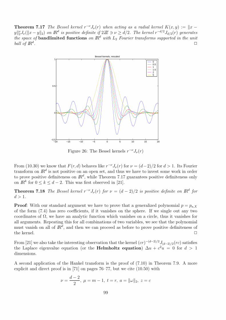
Theorem 7.17 The Bessel kernel r−νJν(r) when acting as a radial kernel K(x, y) := ‖x −y‖ν

2Jν(‖x− y‖2) on IRd is positive definite if 2ZZ ∋ ν ≥ d/2. The kernel r−d/2Jd/2(r) generatesthe space of bandlimited functions on IRd with L2 Fourier transforms supported in the unitball of IRd. 2

−20 −15 −10 −5 0 5 10 15 20−0.5

0

0.5

1Bessel kernels, rescaled

00.511.525

Figure 26: The Bessel kernels r−νJν(r)

From (10.30) we know that F (r, d) behaves like r−νJν(r) for ν = (d−2)/2 for d > 1. Its Fouriertransform on IRd is not positive on an open set, and thus we have to invest some work in orderto prove positive definiteness on IRd, while Theorem 7.17 guarantees positive definiteness onlyon IRk for 0 ≤ k ≤ d− 2. This was first observed in [21].

Theorem 7.18 The Bessel kernel r−νJν(r) for ν = (d − 2)/2 is positive definite on IRd ford > 1.

Proof: With our standard argument we have to prove that a generalized polynomial p = pa,X

of the form (7.4) has zero coefficients, if it vanishes on the sphere. If we single out any twocoordinates of Ω, we have an analytic function which vanishes on a circle, thus it vanishes forall arguments. Repeating this for all combinations of two variables, we see that the polynomialmust vanish on all of IRd, and then we can proceed as before to prove positive definiteness ofthe kernel. 2

From [21] we also take the interesting observation that the kernel (cr)−(d−2)/2J(d−2)/2(rc) satisfiesthe Laplace eigenvalue equation (or the Helmholtz equation) ∆u + c2u = 0 for d > 1dimensions.

A second application of the Hankel transform is the proof of (7.10) in Theorem 7.9. A moreexplicit and direct proof is in [71] on pages 76–77, but we cite (10.50) with

ν =d− 2

2, µ = m− 1, t = r, a = ‖ω‖2, z = c

99

to get∫ ∞

0

rd/2J(d−2)/2(r‖ω‖2)

(r2 + c2)mdr =

‖ω‖m−12 c−m+d/2

2m−1Γ(m)K−m+d/2(c‖ω‖2).

Combining with (7.14) applied to φ(r) = (r2 + c2)−m this yields

Φ(ω) =‖ω‖m−1−(d−2)/2

2 c−m+d/2

2m−1Γ(m)K−m+d/2(c‖ω‖2)

=

(‖ω‖2

c

)m−d/221−m

(m− 1)!K−m+d/2(c‖ω‖2).

7.6.3 Change of Variables

We now introduce t = r2/2 as a new variable, writing a radial basis function Φ as

Φ(·) = φ(‖ · ‖2) = f(‖ · ‖22/2), (7.19)

and we shall use Latin characters f, g, . . . to distinguish the transformed functions from theoriginal ones φ, ψ, etc. Note that going over from Φ to φ and further to f loses the informationon the dimension of the space that we want to work on. But we can take advantage of thisloss and write dimension-dependent operations like Fourier transforms as univariate operationswith a scalar parameter d.

We keep the dimension d in mind and rewrite the d-variate Fourier transform equation (7.14)in terms of the transformed function f to get

Φ(ω) = ‖ω‖−d−22

2

∫ ∞

0f(s2/2)sd/2J d−2

2(s · ‖ω‖2)ds

=∫ ∞

0f(s2

2

)(s2

2

) d−22(s · ‖ω‖2

2

)− d−22

J d−22

(s · ‖ω‖2)s ds

=∫ ∞

0f(s2

2

)(s2

2

) d−22

H d−22

(s2

2 · ‖ω‖22

2

)s ds

with the functions Jν and Hν defined by

(z2

)−νJν(z) = Hν(z

2/4) =∞∑

k=0

(−z2/4)k

k!Γ(k + ν + 1)

for ν ∈ C as in (10.32). If we substitute t = s2/2, we find

Φ(ω) =∫ ∞

0f(t)t

d−22 H d−2

2

(t · ‖ω‖

2

2

)dt

=:(F d−2

2f)

(‖ω‖2/2)

(7.20)

with the general operator

(Fνf)(r) :=∫ ∞

0f(t)tνHν(tr)dt. (7.21)

100

Theorem 7.22 The d–variate Fourier transform of a radial kernel φ with φ(r) = f(r2/2) isgiven by

F(d−2)/2(f)(‖ω‖22/2).

The operator Fν is formally defined for all ν > −1 and sufficiently nice functions f , but wecan extend it to all ν ∈ IR, if we omit terms in the series of Hν that have a singularity of theGamma function in their denominator. However, we want to check its domain of definition withrespect to functions f on IR>0 for ν > −1. Near zero, the function f(t)tν should be absolutelyintegrable, because the analyticity of Hν causes no problems at zero. For large ν this allows amoderate singularity of f at zero. Near infinity we have to check the decay of Hν . But sincethe Bessel functions Jν have a O(t−1/2) behaviour for t→ ∞ due to (10.41), we see that Hν(t)decays like t−ν/2−1/4. Thus we require integrability of f(t)tν/2−1/4 at infinity for ν > −1. Sincewe do not need the weakest conditions, we can simply assume

f(t)tν ∈ L1(IR>0). (7.23)

Note that both Fν and Hν generalize to arbitrary ν ∈ IR, provided that certain restrictions onf like (7.23) hold. Furthermore, by symmetry of radial functions and our definition of Fouriertransforms we have

F−1d−22

= F d−22

for d ∈ IN

on sufficiently smooth functions with sufficient decay. We shall see later that this generalizesto F−1

ν = Fν for all ν ∈ IR, wherever both operators are defined. Please keep in mind thatthe parameter ν is related to the space dimension d via ν = (d − 2)/2. We shall work with νinstead of d for notational simplification. Furthermore, we consider a space Srad of temperedradial functions. It could be defined as a subspace of the space S of d-variate temperedtest functions, comprising all radial test functions after introducing ‖x‖2

2/2 as a new variable.However, we prefer to define it as the space of real-valued functions on [0,∞) that are infinitelydifferentiable such that all derivatives vanish faster than any polynomial at infinity. Takingderivatives of (7.19), one can easily see that this yields a subspace of radial test functions onIRd for all space dimensions d. Conversely, any radial test function Φ in the form (7.19) yieldsa function f that is in Srad. To see this one can proceed inductively, using

∂m

∂ωmj

Φ(ω) = f (m)(‖ω‖22/2)ωm

j + lower derivatives with polynomial factors.

Thus the two notions of S coincide, and each radial function which yields a test function for aspecific space dimension will provide a test function for any dimension. Thus Srad is the properspace to define the operators Fν on, and it clearly contains e−r, which can easily proven to bea fixed point of any Fν , using the definitions (10.32) of Hν and (10.24) of the Gamma function.

7.6.4 Calculus on the Halfline

In the space Srad we can introduce a quite useful generalization of the classical calculusoperations. We start with the family of operators

Iα(f)(r) :=∫ ∞

0f(s)

(s− r)α−1+

Γ(α)ds (7.24)

101

on Srad for all α > 0. The simplest special case is

I1(f)(r) :=∫ ∞

rf(s)ds

with the inverseI−1(f)(r) := −f ′(r).

Note that this operation implies that the resulting function vanishes at infinity, and thus thereis no additive constant in the integration. Furthermore, the identity

Id = In1 In

−1

is Taylor’s formula at infinity, as follows from (7.24). The identity (10.25) allows a direct proofof the property

Iα Iβ = Iα+β (7.25)

for all α, β > 0 by application of Fubini’s theorem. Differentiation and integration by partsimply

In−1 Iα = Iα−n 0 < α < n

In+α In−1 = Iα α > 0, n > 0.

By Iα = Iα In In−1 = In Iα In

−1 we get

In−1 Iα = Iα In

−1,

and this suffices to prove that (7.25) holds for all α, β ∈ IR if we define

I0 := IdI−n := In

−1, n > 0Iα := Iα−⌊α⌋ I⌊α⌋

for the remaining cases of α. Altogether, we have

Theorem 7.26 The operators Iα on Srad form an abelian group under composition which isisomorphic to IR under “+” via α 7→ Iα.

Proof: The remaining things are easy to prove using the above rules. 2

Let us do some simple examples of differentiation and integration of fractional order. Theindependent variable will be denoted by t, and we indicate the domain of validity of the differentcases, because we do not restrict ourselves to tempered radial functions.

Iα(f(t+ x))(r) = Iα(f(t))(r + x) α ∈ IR, x ≥ 0Iα(f(tx))(r) = x−αIα(f(t))(rx) α ∈ IR, x ≥ 0Iα(e−st)(r) = s−αe−sr α ∈ IR, s > 0

Iα(t−βΓ(β))(r) = r−(β−α)Γ(β − α) β > 0, α < βIα((x+ t)−βΓ(β))(r) = (x+ r)−(β−α)Γ(β − α) β > 0, α < β, x > 0

Iα

((s− t)β−1

+

Γ(β)

)(r) =

(s− r)α+β−1+

Γ(α + β)β > 0, α + β > 0

102

We shall make specific use of the “semi-integration” operator and its inverse, the “semi-differentiation”, as given by

I1/2(f)(r) =∫ ∞

r

f(s)√π(s− r)

ds

I−1/2(f)(r) = −∫ ∞

r

f ′(s)√π(s− r)

ds

= I1/2 I−1(f)(r),

(7.27)

that are inverses of each other.

A very simple representation of the operators Iα is possible via the Laplace transform

L(ϕ)(r) :=∫ ∞

0ϕ(s)e−rsds (7.28)

which exists classically for any continuous function ϕ on [0,∞) that grows at most polyno-mially towards infinity. For the time being, we ignore the more general definitions of Laplacetransforms and observe that the action of Iα can be written down as

Iα(L(ϕ)(·)) := L(ϕ(·)(·)−α),

where all real α are formally possible (provided that ϕ behaves nicely enough).

7.6.5 Basic Transitions

The main advantage of Srad and the definition (7.21) of the radial Fourier transform using(7.20) is that we can compare Fourier transforms for various dimensions, while working on asimple space of univariate functions. But the most surprising fact, as discovered by Wu, showsup when we simply take the derivative of Fν(f)(r). We use (10.34) to get

− d

drFν(f)(r) = (I−1 Fν)(f)(r)

= − d

dr

∫ ∞

0f(t)tνHν(rt)dt

= −∫ ∞

0f(t)tν

d

drHν(rt)dt

=∫ ∞

0f(t)tν+1Hν+1(rt)dt

= Fν+1(f)(r).

(7.29)

Going back to ν = (d − 2)/2, we see that the (d + 2)-variate Fourier transform of a radialfunction after the substitution (7.19) is nothing else than the negative univariate derivative ofthe d-variate Fourier transform after (7.19). We shall generalize the above identity later toIα Fν = Fν−α on R, but we already know that I1 Fν = Fν+1 allows to proceed from (d+ 2)-variate radial Fourier transforms to d-variate Fourier transforms by univariate integration.

103

Let us apply (10.35) to get another identity on tempered functions:

Fν(−f ′)(r) =∫ ∞

0−f ′(s)sνHν(sr)ds

=∫ ∞

0f(s)sν−1Hν−1(sr)dsdt

= = Fν−1(f)(r).

(7.30)

This will generalize to Fν Iα = Fν+α and is a trivial consequence of Iα Fν+α = Fν andF 2

µ = Id, if the latter holds in general.

Note that in both cases we have operators that preserve compact supports. The integraloperator even preserves nonegativity (it is a monotone operator). The explicit constructionof compactly supported radial functions relies heavily on these features. But we also want toproceed from d-variate Fourier transforms to (d+1)- or (d−1)-variate Fourier transforms. Thiswill be achieved by the operator I1/2 and its inverse from (7.27). We shall treat this problemin general, comparing two arbitrary instances Fν and Fµ.

7.6.6 Identities for Transforms, First Version

We can easily evaluate the action of the Fourier operator on the Laplace transform as

Fν(L(ϕ))(r) =∫ ∞

0sνHν(sr)

∫ ∞

0ϕ(t)e−stdtds

=∫ ∞

0ϕ(t)

∫ ∞

0sνHν(sr)e

−stdsdt

=∫ ∞

0ϕ(t)t−ν−1

∫ ∞

0xνHν(xr/t)e

−xdxdt

=∫ ∞

0ϕ(t)t−ν−1e−r/tdt

=∫ ∞

0ϕ(1/s)sν−1e−srds

= L (ϕ(1/·)(·)ν−1) .

Then, again as formal operations,

Fν(L(ϕ(·))) = L (ϕ(1/·)(·)ν−1)= Iµ−νL (ϕ(1/·)(·)µ−1)= Iµ−νFµ(L(ϕ(·)),

Fν(Fµ(L(ϕ(·)))) = Fν (L (ϕ(1/·)(·)µ−1))= L (ϕ(·)(·)−µ+1(·)ν−1)= Iµ−ν(L(ϕ(·))),

as expected. Note that this implies F 2ν = Id for all ν. All of these identities are valid at least

on Laplace transforms of functions ϕ that vanish faster than any polynomial at zero and atinfinity, but continuity arguments can be used to enlarge the scopes.

104

7.6.7 Identities for Transforms, Second Version

The previous section showed that the identity

Fν Fµ = Iµ−ν

holds for all µ, ν ∈ IR on a small space of functions, and where Iα is an operator that roughlydoes α-fold integration for α ∈ IR. We now want to make this more precise and explicit. Inparticular, we assert F 2

ν = Id for all ν, which we only know for ν ∈ 12ZZ>−2. Furthermore, we

want to use our explicit representations for the operators Iα.

To proceed towards inversion of the operator Fν , let us start calculating the Fourier transform ofthe simplest compactly supported function, i.e.: a truncated power. The outcome is somewhatsurprising, because we run into the function Hν again:

Lemma 7.31 For ν > µ > −1 and all s, r ≥ 0 we have

Fµ

(s−ν(s− ·)ν−µ−1

+

Γ(ν − µ)

)(r) = Hν(rs).

Proof: We directly calculate the assertion and use (10.36) from page 153. In detail,

Fµ

(s−ν(s− ·)ν−µ−1

+

Γ(ν − µ)

)(r)

=∫ ∞

0tµs−ν(s− t)ν−µ−1

+

Γ(ν − µ)Hµ(tr)dt

= s−ν

Γ(ν − µ)

∫ s

0tµ(s− t)ν−µ−1Hµ(tr)dt

= s−ν

Γ(ν − µ)

∫ s

0tµ(s− t)ν−µ−1Jµ(2

√rt)(rt)−µ/2dt,

and by substitution t = su2, we get

= s−ν

Γ(ν − µ)

∫ 1

0sµu2µsν−µ−1(1 − u2)ν−µ−1Jµ(2

√rsu)(rsu2)−µ/22sudu

=2(rs)−µ/2

Γ(ν − µ)

∫ 1

0uµ+1(1 − u2)ν−µ−1Jµ(2

√rsu)du

=2(rs)−µ/2

Γ(ν − µ)2ν−µ−1Γ(ν − µ)

(2√rs)−ν−µ Jν(2

√rs)

= (√rs)−νJν(2

√rs)

= Hν(rs).

2

We would like to invert the Fourier transform in the above assertion, but the decay of Hν is notsufficient to see directly that Fµ is applicable at all. However, we can resort to specific toolsfrom Special Functions to get

105

Lemma 7.32 For ν > µ > −1 and all r, s > 0 we have

(FµHν(s·))(r) =s−ν(s− r)ν−µ−1

+

Γ(ν − µ).

Proof: The assertion is a consequence of the Weber–Schafheitlin integral (see (10.44) or[1] p. 487, 11.4.41) after substitutions of the type t = s2/2. In detail, we have

(FµHν

(u2

2 ·))(

r2

2

)

=∫ ∞

0tµHµ

(r2

2 t)Hν

(u2

2 t)dt

=∫ ∞

0

(s2

2

)µ

· s ·Hµ

(r2

2 · s2

2

)Hν

(u2

2 · s2

2

)ds

=∫ ∞

02−µs2µ+1

(rs2

)−µ(us2

)−νJν(us)ds

= 2νr−µr−ν∫ ∞

0sµ−ν+1Jµ(rs)Jν(us)ds

=2νr−µu−ν2µ−ν+1rµ(u2 − r2)ν−µ−1

+

uνΓ(ν − µ)

= 1Γ(ν − µ)

(u2

2

)−ν

(u2

2 − r2

2

)ν−µ−1+ .

2

The above result can be used to derive the d–variate Fourier transform of the kernel

K(x, y) := Hν

(c2‖x− y‖2

2

4

)=

(c‖x− y‖2

4

)−ν

Jν

(c‖x− y‖2

2

)(7.33)

We have to rewrite this kernel as φ(r) = f(r2/2) and get

f(t) = Hν

(c2

2t

).

Then the above lemma yields

(F(d−2)/2Hν

(c2

2·))(

‖ω‖22

2

)=

(c2

2

)−ν (c2

2− ‖ω‖2

2

2

)ν−d/2

+

Γ(ν − d/2 + 1)(7.34)

proving

Theorem 7.35 If 2ν + 2 > d holds, the scaled Bessel kernel (7.33) is positive definite on IRd

and has the compactly supported Fourier transform (7.34) due to Theorems 7.22 and 7.7.

We now know that Fν Fν = Id holds on Laplace transforms, on truncated powers, and onfunctions of the form Hµ(s·). But before we generalize this to a larger class of functions, wegeneralize it to other Fµ operators:

106

Theorem 7.36 Let ν > µ > −1. Then for all tempered radial test functions f ∈ Srad we have

Fµ Fν = Iν−µ (7.37)

where the integral operator Iα is given by

(Iαf)(r) =∫ ∞

0f(s)

(s− r)α−1+

Γ(α)ds, r > 0, α > 0.

Proof: For any tempered radial test function f ∈ Srad we evaluate (Fµ · Fν)f(r) by means ofLemma 7.32 to obtain

∫ ∞

0Hµ(tr)tµ

∫ ∞

0Hν(st)s

νf(s)dsdt

=∫ ∞

0sνf(s)

∫ ∞

0tµHµ(tr)Hν(ts)dt ds

=∫ ∞

0sνf(s) · Fµ(Hν(s·))(r)ds

=∫ ∞

0f(s)

(s− r)ν−µ−1+

Γ(ν − µ)ds = (Iν−µf)(r).

2

By the above theorems it is easy to see that

IαHν = Hν−α

for all α < ν + 1, generalizing (10.34).

7.6.8 Wendland’s Functions

Due to a result of Askey [4] the radial truncated power function

Aµ(·) := (1 − ‖ · ‖2)µ+

is positive definite on IRd for µ ≥ ⌊d/2⌋ + 1, because it has a strictly positive radial Fouriertransform in this case.

Incomplete: add proof see [71]

Its radial form after substitution is (1−√

2r)µ+, and due to its finite support we can apply any

Fν operator for ν > −1. We use the identity Fν+α = Fν Iα from (7.30) for this function andget

Fν+kAµ = Fν(Ik(Aµ)), k ∈ IN,

where the left-hand side is strictly positive whenever

µ ≥ ⌊d/2⌋ + 1 + k. (7.38)

Thus the function Ik(Aµ) is positive definite on IRd for the same range of parameters. Sincethe Ik operators preserve compact supports, the resulting functions

ψµ,k(r) := Ik(Aµ(r2/2))

107

lead to compactly supported positive definite functions

Ψµ,k(·) = ψµ,k(‖ · ‖2) = Ik(Aµ(‖ · ‖22/2))

on IRd under the condition (7.38). Let us do a straightforward evaluation. This yields

IkAµ(r) =∫ ∞

0(1 −

√2s)µ

+

(s− r)k−1+

(k − 1)!

=∫ 1

√2rt(1 − t)µ (t2/2 − r)k−1

+

(k − 1)!

=∫ 1

xt(1 − t)µ (t2 − x2)k−1

+

(k − 1)!2k−1

(7.39)

for 0 ≤ r ≤ 1/2 or 0 ≤ x =√

2r ≤ 1. If µ is an integer, the resulting function is a singlepolynomial of degree µ + 2k in the variable x = ‖ · ‖2 on its support. The case k = 1 isparticularly simple. We get the explicit representation

I1Aµ(x2/2) =∫ 1

xt(1 − t)µdt

=x(1 − x)µ+1

µ+ 1+

(1 − x)µ+2

(µ+ 1)(µ+ 2)

=(1 − x)µ+1

+

(µ+ 1)(µ+ 2)(1 + (µ+ 1)x) .

The smallest possible integer µ for d ≤ 3 and k = 1 is µ = 3, whence

I1A3(x2/2) =

1

20(1 − x)4

+(1 + 4x).

In addition to Ak,µ := IkAµ let us define

Bk,µ :=∫ 1

x(1 − t)µ (t2 − x2)k−1

+

(k − 1)!2k−1

and split the integral defining Ak,µ via t = (t− 1) + 1 into

Ak,µ = −Bk,µ+1 +Bk,µ.

Then do integration by parts for Bk,µ and k > 1 to get

Bk,µ =1

µ+ 1Ak−1,µ+1.

Thus we have the recurrence relation

Ak,µ = − 1

µ+ 2Ak−1,µ+2 +

1

µ+ 1Ak−1,µ+1.

Looking at our result for k = 1 we see that we can assume

Ak,µ(x2/2) = (1 − x)µ+kCk,µ(x)

108

with the recursion

Ck,µ(x) =(x− 1)

µ+ 2Ck−1,µ+2(x) +

1

µ+ 1Ck−1,µ+1(x),

for k ≥ 1, starting withC0,µ(x) = 1.

Thus the polynomials Ck,µ have degree k with a positive leading coefficient. The number ofcontinuous derivatives of Ak,µ(x

2/2) at x = 1 thus is µ+ k − 1 ≥ 2k + ⌊d/2⌋ ≥ 2k. To get thenumber of derivatives at zero we apply the binomial theorem to the last factor in the integrand.Then

Ak,µ(x2/2) =

k−1∑

j=0

(k − 1j

)(−1)jx2j

(k − 1)!

∫ 1

xt(1 − t)µt2k−2−2jdt

qµ,k−j(x) :=∫ 1

xt(1 − t)µt2k−2−2jdt

= qµ,k−j(1) −∫ x

0t(1 − t)µt2k−2−2jdt

= qµ,k−j(1) − x2k−2j

2k − 2j+ higher-order terms

shows that the first odd monomial occurring in Ak,µ(x2/2) cannot have an exponent smaller

than 2k+1. Thus the function has 2k continuous derivatives at zero, and we get 2n−1 = 2k+1in the context of Wendland’s functions. In terms of continuity requirements, we get overall C2k

continuity at a minimal degree µ+ 2k = ⌊d/2⌋+ 3k+ 1, and Wendland proves in [70] that thisdegree is minimal, if we ask for a single polynomial piece on [0, 1] that induces a positive definiteradial function which is C2k and positive definite on IRd. Note that the order of smoothness atthe boundary of the support is ⌊d/2⌋ larger than the smoothness at zero, which has a positiveeffect on the visual appearance of the reproduced functions.

We end this by giving the C4 case for all dimensions d, where µ = ⌊d/2⌋ + 3:

A2,µ(x2/2)

=(1 − x)µ+2

+

(µ+ 1)(µ+ 2)(µ+ 3)(µ+ 4)(x2(µ+ 1)(µ+ 3) + 3x(µ+ 2) + 3)

and the most frequent case for d ≤ 3 is

A2,4(x2/2) =

(1 − x)6+

1680(35x2 + 18x+ 3).

The Fourier transforms areFνIkAµ = Fν+kAµ

and thus for r = x2/2 of the form

Fν+kAµ(r) =∫ 1/2

0(1 −

√2s)µsν+kHν+k(rs)ds

=x−ν−k

2ν+k

∫ 1

0(1 − t)µtν+k+1Jν+k(xt)dt

=x−µ−2ν−2k−2

2ν+k

∫ x

0(x− u)µuν+k+1Jν+k(u)du.

109

Due to a result of Gasper [23], the above integral can be written as a positive sum of squaresof Bessel functions, at least in the odd-dimensional case d = 2n− 1 with µ = n+ k + 1, whichleads to ν = m− 1/2 and µ = m+ 1 for m = n+ k ≥ n. Results of Wendland [70] then implythe asymptotic behaviour

FνIkAµ(r2/2) = Fν+kAµ(r2/2) ≥ cr−d−2k−1

for the necessary values of µ from (7.38).

7.7 Conditionally Positive Definite Kernels

We now go over to the treatment of general unconditionally positive definite kernels. To dothis, we shall introduce Fourier transforms in a somewhat more general way that will latersave us quite some work. The direct attack is impossible, because some of the most importantconditionally positive definite functions on IRd are radial functions Φ(·) = φ(‖ · ‖2) that growtowards infinity, e.g.: thin-plate splines φ(r) = r2 log r or multiquadrics φ(r) =

√r2 + c2.

These do not have classical Fourier transforms, but since they grow at most polynomially, theyinduce functionals on the Schwartz space S. Thus they have generalized Fourier transformsdefined via the Fourier transforms of the functionals that they induce on S. These generalizedFourier transforms are not straightforward to handle and require quite some machinery fromdistribution theory.

We go a different way by picking a very specific set of assumptions to start with, and then we canwork our way without distributions. We do not even assume Φ to be a conditionally positivedefinite function; this will be a consequence of our assumptions and lead to an importanttechnique to prove conditional positive definiteness for specific examples.

In what follows, recall the notation used in section 4.3, but here we fix the space IP to be thespace IP d

m of d–variate polynomials of order at most m. Furthermore, we use the notion ofFourier transforms of functionals as provided in section 10.5.

Assumption 7.40 Let Φ : IRd → IR be even and continuous. Furthermore, let there be acontinuous nonnegative function

Φ : IRd \ 0 → IR

which is positive on at least an open set. It may possibly have an algebraic singularity

Φ(ω) = O(‖ω‖−d−β0) (7.41)

with some real value β0 for ω near zero, and it must have the behavior

Φ ∈ L1 near infinity. (7.42)

Then define m := max(0, ⌊β0⌋) ≥ 0 to get the restriction

β0 < 2m (7.43)

that will often occur later. Finally, let the usual bilinear form on L be representable by

(λa,X , λb,Y )Φ = (2π)−d/2∫

IRdΦ(ω)

M∑

j=1

N∑

k=1

ajbkei(xj−yk)·ωdω, (7.44)

110

where the functionals λa,X ∈ L satisfy the moment conditions (4.18) in the form

λa,X(IP dm) = 0, (7.45)

and thus we may use the notation (IP dm)⊥

IRd for L.

Lemma 7.46 The functionals λa,X ∈ L have Fourier transforms

λa,X(ω) = pa,X(ω) =N∑

j=1

aje−ixT

j ω

with zeros of order at least m in the origin.

Proof: Since we have (7.45), we can use Example 10.21 to get our result. 2

Theorem 7.47 Under the above assumptions the function Φ(x − y) is conditionally positivedefinite of order ≥ m on IRd.

Proof: From the previous lemma we know that the functionals λa,X ∈ L have Fourier trans-forms with zeros of order at least m in the origin. Thus the integrand in (7.44) is of orderO(‖ω‖2m−d−β0) near zero, and the integral is well-defined due to (7.43) and (7.42). Nonnega-tivity of Φ proves that the bilinear form is positive semidefinite. The rest is as in the proofs ofTheorems 7.6 and 10.7. 2

The reader should be aware that we did not assume Φ to be the usual Fourier transform. Wethus cannot use equations (10.6) or (10.11), but we have the general identity

M∑

j=1

N∑

k=1

ajbkΦ(xj − yk) = (2π)−d/2∫

IRdΦ(ω)

M∑

j=1

N∑

k=1

ajbkei(xj−yk)·ωdω.

that is identical to (7.44) and is valid for all functionals in L due to Assumption 7.40. It willnicely serve as a substitute for (10.11), but note that it does not allow single point-evaluationfunctionals in the left-hand side.

7.8 Examples

We now present special cases of (7.44) for radial kernels

K(x, y) = Φ(x− y) = φ(‖x− y‖2), x, y ∈ IRd

where we get a resulting generalized d–variate Fourier transform in radial form which we denoteby φ.

The first example generalizes the inverse multiquadrics to general multiquadrics. If we set

φ(r) := (c2 + r2)β/2, r ≥ 0, c > 0, β ∈ IR \ 2IN 0

we get the function

φ(s) =21+β/2

Γ(−β/2)(s

c

)−β+d2

Kβ+d

2(cs), s ∈ IR

111

while the order of conditional positive definiteness turns out to be

m = max(0, ⌈β/2⌉).

Note that for positive β the denominator has the sign (−1)⌈β/2⌉. Thus we have to multiply φfor positive β with this factor to get a conditionally positive definite function.

The proof idea is quite nice. Each side of the standard Fourier transform identity (7.44),including the quadratic form and holding first for negative β is proven to be an analytic functionof β. Under the additional moment conditions, both sides also make sense for general β, andthey can be connected by analytic continuation with the case for negative β by a detour overcomplex β avoiding passing through the origin. Thus the Fourier transform equation also holdsfor the other β.

The next example concerns the power functions, and this is the limit of the previous case forc→ 0. If we set

φ(r) := (−1)⌈β/2⌉rβ, r ≥ 0, β ∈ IR>0 \ 2IN

we get the positive function

φ(s) =2β+d/2Γ((β + d)/2)

(−1)⌈β/2⌉Γ(−β/2)s−β−d, s ∈ IR


m = ⌈β/2⌉.

This proof works from the previous case for positive β by letting c tend to zero, checkingcarefully how the Bessel function interacts with the premultiplied rational function.

The final case is connected to β being an even integer. If we set

φ(r) := (−1)k+1r2k log r, r ≥ 0, k ∈ IN

we getφ(s) = 22k−1+d/2s−2k−d, s ∈ IR


m = k + 1.

The last two cases are called polyharmonic, because they are homogeneous solutions of apower of the Laplacian. This is due to the fact that their generalized Fourier transform is aplain negative power. The last case is called the thin–plate spline.

7.9 Connection to L2(IRd)

We now go back to Definition 4.41 of the native space via (4.42) and Corollary 4.43as

NK,Ξ := IP dm +G = IP d

m + F .

112

This definition is very general, and we want to re–express the native space via Fourier trans-forms. We do this using a detour over weighted L2 spaces.

The space L of section 4.3 consists of functionals λa,X with the moment condition (a,X) ∈M .

These functionals have Fourier transforms λa,X with the property

λa,X(f) = (2π)−d/2(f , λa,X)L2(IRd), (λa,X)(ω) =N∑

j=1

aje−ixT

j ω.

Assumption 7.40 makes sure that the mapping

L : λ 7→ λ

√Φ, L = (IP d

m)⊥IRd → L2(IRd)

is well-defined. Indeed, the function L(λ) is in L2 near infinity due to (7.42), and it is continuousaround zero due to (7.43), since λ has a zero of order at least m at the origin.

With the results of the previous section, (7.44) takes the form

(λa,X , λb,Y )Φ = (2π)−d/2(Lλa,X ,Lλb,Y )L2(IRd). (7.48)

Theorem 7.49 Let Assumption 7.40 be satisfied, and let m be minimal with respect to (7.43).Then the map L extends by continuity to clos (L), and it yields an isometry between clos (L)and all of L2(IR

d).

Proof: It is evident from (7.44) that L is isometric, and thus L extends to clos (L) by continuity.But the density of L( clos (L)) in L2(IR

d) does not follow from abstract Hilbert space arguments.We thus need an additional analytic argument. We first prove the assertion for continuous Φwith Φ > 0 on IRd \ 0.

Let some function f ∈ L2(IRd) and some ε > 0 be given. Then there is a compactly supported

C∞ function g ∈ L2(IRd) such that ‖f − g‖2 ≤ ε due to Lemma 10.4. Now define u := g/

√Φ

on IRd, where the (possible) singularity of Φ at zero does no harm. Clearly u is continuousand compactly supported, thus in L2(IR

d) and u is band–limited, of exponential type, andin L2(IR

d). We now invoke the multivariate sampling theorem to recover u exactly from itsfunction values on a grid in IRd with spacing h, where h is sufficiently small and related to thesupport of u.

Thus we have

u(x) =∑

j∈ZZd

u(jh) Sincd

(x− jh

h

), x ∈ IRd

where

Sincd(x1, . . . , xd) =d∏

j=1

sin πxj

πxj,

andu(ω) =

∑

j∈ZZd

u(jh)eihj·ω, ω ∈ IRd

113

has the form u = λu for the functional

λu(v) =∑

j∈ZZd

v(jh)u(jh).

We now have to make sure that λu ∈ clos (L). If this is done, we are finished because ofL(λu) = g and

‖f −√

Φλu‖2 = ‖f − g‖2 ≤ ε.

For all p ∈ IP dm we have to show that λu(p) = 0. By a standard argument in Fourier analysis

this requires a zero of order at least m of u at zero. But our assumption (7.41) on Φ and theminimality of m in (7.43) imply that u has a zero of order at least

1

2(d+ β0) >

1

2(d+ 2m− 2) = m− 1 +

d

2,

thus of order ≥ m.

We then evaluate the norm formally as

‖λu‖2Φ = ‖

√Φ · λu‖2

2 = ‖√

Φu‖22 = ‖g‖2

2 <∞.

Now we can proceed to prove that λu lies in clos (L) by defining the function

fλu(x) := (λu, δx,Ξ)Φ, x ∈ IRd

via the explicit form of the inner product, and using the finiteness of the norm ‖λu‖Φ to showthat the definition is valid. Then for all λY,N,β ∈ L we get

λY,N,β(fλu) = (λu, λY,N,β)Φ

and this proves that fλu ∈ F . Finally, we get λu = F−1(fλu) by checking

(λu, λY,N,β)Φ = λY,N,β(fλu)

= (λY,N,βF−1fλu))Φ

for all λY,N,β ∈ L, and this concludes the proof in case of Φ > 0.

Now let Φ be positive up to a set of Lebesgue measure zero. We cover the set of zeros byintervals Ik, where k varies over some index set K and the total area

∑k |Ik| is less than some

given δ. Now let Φδ(ω) ≥ Φ(ω) be a strictly positive continuous function that differs from Φonly on the Ik. Then Φδ will also satisfy our assumptions, and we can use (7.44) in the form

(µ, λ)Φδ:= (2π)−d/2

∫

IRdΦδ(ω)λ(ω)µ(ω)dω

as a definition of an inner product, but we do not need Φδ explicitly.

Now we approximate a given f ∈ L2(IRd) by some

√Φδ · λ up to ε/2 in the L2 norm, picking

a suitable λ for each δ and ε. Then

‖f −√

Φλ‖2 ≤ ‖f − λ√

Φδ‖2 + ‖λ(√

Φδ −√

Φ)‖2

114

and

‖λ(√

Φδ −√

Φ)‖22 = ‖λ ·

√Φδ(1 −

√Φ/Φδ)‖2

2

≤∑

k

∫

Ik

|λ(ω)|2Φδ(ω)dω.

The full integral ∫

IRd|λ(ω)|2Φδ(ω)dω = ‖λ ·

√Φδ‖2

2

can be bounded independent of δ, because it approximates ‖f‖22. Thus we are able to pick δ

small enough to guarantee∑

k

∫

Ik

|λ(ω)|2Φδ(ω)dω ≤ ε/2

yielding an overall bound ‖f −√

Φλ‖2 ≤ ε. 2

7.10 Characterization of Native Spaces

We now can re–express the native space NK,Ξ := IP dm +G = IP d

m + F . via Fourier transforms.

Theorem 7.50 The native space NK,Ξ := IP dm+G for a conditionally positive definite function

of order m on IRd satisfying Assumption 7.40 coincides with the space of all functions f on IRd

that can be written as

fh(x) = (2π)−d/2∫

IRdh(ω)

√Φ(ω)

eix·ω −Q∑

j=1

pj(x)eiξj ·ω

dω (7.51)

plus polynomials from IP dm and where h ∈ L2(IR

d). The above functions are spanning the spaceG. The bilinear form on G can be rewritten as

(fg, fh)Φ = (2π)−d/2(g, h)L2(IRd). (7.52)

Proof: We first focus on (7.51). Starting with an arbitrary h ∈ L2(IRd) and a fixed IP d

m-unisolvent set Ξ ⊂ IRd, we mimic the technique of Riesz maps to define a function

fh(x) := (h,Lδ(x))L2(IRd). (7.53)

This is (7.51). Sinceλfh = (h,Lλ)L2(IR

d)

follows easily from (7.52) for all λ ∈ L, we can transform this equation further into

λfh = (h,Lλ)L2(IRd)

= (L−1h, λ)Φ.

By the previous section, (7.48) with Theorem 7.49 yields that L−1 maps L2(IRd) isometrically

back to L. But L is isometric to G via the extension R of the Riesz map R : L → G we hadin section 4.5. Thus the above identity can be extended to

λfh = (h,Lλ)L2(IRd)

= (L−1h, λ)Φ

= (RL−1h,Rλ)Φ for all λ ∈ L

115

provingfh = RL−1h ∈ G.

2

By (??) we also get

Corollary 7.54 The mappingF = RL−1 : h 7→ fh

is isometric between L2(IRd) and G. 2

Note that we avoided to use the Fourier transform of fh. In case that√

Φh =: gh is an absolutelyintegrable function, the right–hand side of (7.51) is

fh(x) = g∨h (x) −Q∑

j=1

pj(x)g∨h (ξj)

such that we see that a polynomial variation of fh has a Fourier transform which is√

Φh.

But we can also work via the F part of the native space. It is the closure of all functions

fa,X(x) := λta,XΦ(x− t),

and if the functional is such that Fourier tyransforms can be taken, we get

fa,X = Φλa,X =

√ΦLλa,X

such thatfa,X√

Φ= Lλa,X ∈ L2(IR

d).

This can also be written as

R(λ)∧ = λ =

√ΦL(λ)

if all transforms exist, and this is a third reason to define

fh :=

√Φh

as a generalized Fourier transform of fh, but the use of standard Fourier transform equationsis forbidden without additional argumants along the above lines.

7.11 Connection to Sobolev Spaces

To make error bounds applicable, we need inclusion theorems for native spaces in Sobolevspaces. Since polynomials are not contained in global Sobolev spaces, we can only expect theG part of the native space to be contained in a global Sobolev space W τ

2 (IRd), while polynomialsare always contained in local Sobolev spaces W τ

2 (Ω) for bounded domains. Thus we cannotwork as easily as in the unconditionally positive definite case.

116

Let us check the differentiability of the functions from (7.51). Under sufficient regularity of√Φh =: gh, we take a derivative Dα of fh of order α with |α| ≥ m. It will have Fourier

transform (iω)α

√Φ(ω)h(ω) and we check when it is well–defined and globally in L2. This is

the case when ‖ω‖2|α|Φ(ω) is globally bounded. Since we only use L2 arguments for this result,

we can ignore the additional regularity assumptions on√

Φh =: gh by an additional densityargument.

Near zero, the boundedness of ‖ω‖2|α|Φ(ω) follows for

2|α| ≥ d+ β0

because‖ω‖2|α|Φ(ω) ≤ O(‖ω‖2|α|−d−β0).

Near infinity, we have not yet made any assumptions about the behavior of Φ. For simplicity,we mimic (7.41) as

Φ(ω) ≤ O(‖ω‖−d−β∞) near ∞. (7.55)

Then a sufficient condition for boundedness at infinity is

2|α| ≤ d+ β∞.

Altogether, we get that the derivative Dαfh is defined and globally in L2 at least for

|α| ≥ m, β0 + d ≤ 2|α| ≤ β∞ + d.

This is quite sufficient for the multiquadric case, because there β∞ is arbitrarily large. For thethin–plate spline and the polyharmonic splines, we have β0 = β∞ and see that we can still workwith generalized derivatives of order m = |α| = d/2 + β∞/2 = d/2 + β0/2 > d/2 if this is aninteger.

In all of these cases we can take the maximum possible |α| and get convergence of interpolantslike h|α|−d/2 in the L∞ norm when the data are from a function in the native space. This yieldsinfinite order for the multiquadrics and convergence like hβ0/2 = hβ∞/2 for the thin–plate splineand the polyharmonic spline provided that d+ β0 = d+ β∞ is even.

incomplete here...

8 Stability Theory

It would be very desirable to have recovery methods with small errors and good stability.However, these two goals cannot be met at the same time, since there is a connection betweenthem that implies bad stability whenever the a-priori error bound is very small.

117

8.1 Uncertainty Relation

Let us look at this connection in the Lagrange interpolation setting and consider optimalrecovery of a function g ∈ N in a Hilbert space N which is the native space of a reproducingkernel K on a domain Ω ⊂ IRd. This recovery should use data g(xj), 1 ≤ j ≤M for a finite setX = x1, . . . , xM ⊂ Ω ⊂ IRd.

We add a variable point x to X and define the kernel matrix

Ax,X :=

Φ(x, x) Φ(x, x1) . . . Φ(x, xM )Φ(x1, x) Φ(x1, x1) . . . Φ(x1, xM)

......

...Φ(xM , x) Φ(xM , x1) . . . Φ(xM , xM)

and the vector(u∗X)T (x) := (1,−u∗1(x), . . . ,−u∗M(x))T ∈ IRM+1

with the Lagrange basis of (3.4) and get the special form

P 2X(x) = K(x, x) − 2

N∑

j=1


j,k=1

u∗j(x)u∗k(x)K(xj , xk)

= (u∗X)T (x)Ax,X(u∗X)(x)

≥ σ(Ax,X)

1 +

M∑

j=1

|u∗j(x)|2

≥ σ(Ax,X)

(8.1)

of the power function (3.8), where σ(Ax,X) is the minimal eigenvalue of Ax,X. Note that bothsides are continuous functions of x and X (or Λ standing for X) that vanish whenever x tendsto points in X.

Theorem 8.2 The error of kernel interpolation can only be small if the condition of the kernelmatrix is large. In particular,

P 2X(x) ≥ σ(Ax,X)

holds for the power function P 2X in terms of the smallest eigenvalue σ(Ax,X) of the kernel matrix

Ax,X.

We can call the above observation an Uncertainty Principle or a Tradeoff principle.

The interpretation of the above result is as follows. Assume we have a recovery process witha very good error bound (3.7) via the power function. Then Ax,X must have a very smalleigenvalue. The largest eigenvalue of Ax,X can only be as large as a constant times N , thus it isnot very relevant for the condition of Ax,X , which is the quotient of the largest by the smallesteigenvalue, if the condition is taken in the spectral norm. Thus the condition of Ax,X is largewhenever the recovery error is small. But Ax,X is itself a kernel matrix, if we view x as the“‘next” interpolation point. Or, when we change the meaning of x and X somewhat, we canrewrite the above result as

min1≤j≤N

P 2X\xj

(xj) ≥ σ(AX),

bounding the smallest eigenvalue of a kernel matrix via the “leave–one–out” power function.

118

We now can give some hints to the results that follow in later sections. The UncertaintyRelation in the form (8.1) suggests to bound P 2 from above and σ from below, in order to haveboth upper bounds on the attainable error and on the numerical stability, measured by 1/σ.We have seen in the previous chapter that upper bounds for P 2 take the form

P 2Xh

(x) ≤ F (hX,Ω) for all x ∈ Ω (8.3)

where F is a monotonic function of the fill distance hX,Ω defined in (5.2). On the other hand,the lower bounds for σ which we shall prove in this chapter, will be of the form

σ(AX) ≥ G(qX) for all X = x1, . . . , xM ⊂ Ω (8.4)

with the separation distance

q := qX := min1≤i6=j≤M

‖xi − xj‖2. (8.5)

For gridded data on ǫZZd ∩ Ω we can roughly expect hX,Ω = qX√d, and then the Uncertainty

Relation necessarily impliesF (t

√d) ≥ G(t) (8.6)

for all t ≥ 0. This allows to check the quality of the bounds (8.3) and (8.4), since the lowestpossible bounds F and the largest possible bounds G must necessarily satisfy (8.6) and areoptimal, if they turn (8.6) into an equality. This opens the race for optimal bounds of the form(8.3) and (8.4), and this text will describe the current state-of-the-art. To cut the story short,we shall prove that F and G just differ by a factor in case of kernels of finite smoothness, i.e.(8.6) is extended to

F (t√d) ≥ G(t) ≥ C · F (c · t) (8.7)

for all t ≥ 0, proving that the square of the power function and the minimal eigenvalue of thekernel matrix are roughly proportional in all cases of finite smoothness.

8.2 Lower Bounds on Eigenvalues

This section uses Fourier transform techniques to prove results concerning the condition of thematrices that occur in the basic equations (3.2) and (4.10) for optimal recovery. This requiresupper bounds for the largest, and lower bounds for the smallest eigenvalue. We start withthe latter and restrict ourselves to the Lagrange case. The bounds should (if possible) shouldneither depend on the specific data locations X = x1, . . . , xM, nor on the number M of datapoints, but rather on certain real-valued quantities like the separation distance (8.5).

We generalize the technique of Narcowich and Ward [44] [45] [46] for calculating stabilitybounds, but we introduce Fourier transforms right from the start, which makes it much easierto treat large values of m, the order of conditional positive definiteness of Φ.

The starting point is that any conditionally positive definite function Φ of order m satisfyingAssumption 7.40 allows the formula

M∑

j=1

M∑

k=1

αjαkΦ(xj − xk) = (2π)−d/2∫

IRdΦ(ω)

∣∣∣∣∣∣

M∑

j=1

αjeixj ·ω

∣∣∣∣∣∣

2

dω (8.8)

119

for all IP dm–nondegenerate sets X = x1, . . . , xM and all vectors α ∈ IRM such that λX,M,α is

a functional that annihilates IP dm. This is just another way of writing (7.44).

The left–hand side of (8.8) is the quantity αTAX,Φα that we want to bound from below, andwe can do this by any minorant Ψ on IRd \ 0 of Φ that satisfies

Φ(ω) ≥ Ψ(ω) on IRd \ 0 (8.9)

and that itself leads to a similar quadratic form

M∑

j=1

M∑

k=1

αjαkΨ(xj − xk) = (2π)−d/2∫

IRdΨ(ω)

∣∣∣∣∣∣

M∑

j=1

αjeixj ·ω

∣∣∣∣∣∣

2

dω (8.10)

for another basis function Ψ and a weaker constraint on α ∈ IRM (or none at all). Furthermore,there should be an easy lower bound

αTAX,Ψα ≥ σ‖α‖22

for the left–hand side αTAX,Ψα of (8.10). Then clearly for all α ∈ IRM that are admissible,

αTAX,Φα ≥ αTAX,Ψα ≥ σ‖α‖22,

as required. The basic trick of Narcowich and Ward now is to make AX,Ψ diagonally dominant,while Ψ is obtained by chopping off Φ appropriately near infinity.

Before we proceed any further, here is the main result:

Theorem 8.11 Let Φ be a conditionally positive definite function on IRd that satisfies As-sumption 7.40. Furthermore, let X = x1, . . . , xM ⊂ IRd be any set of Lagrange data locationshaving separation distance (8.5). With the function

φ0(r) := inf‖ω‖∞≤2r

Φ(ω), (8.12)

the smallest eigenvalue σ of the quadratic form associated to the matrix

AX,Φ = (Φ(xj − xk))1≤j,k≤M ,

restricted as usual to the subspace of IRM that contains the coefficient vectors α of functionalsλX,M,α ∈ P⊥

Ω has the lower bound

σ ≥ 1

2

φ0(K)

Γ (d/2 + 1)

(K√2

)d

(8.13)

for any K > 0 satisfying

K ≥ 4

q

(2πΓ2 (d/2 + 1)

) 1

d+ 1 (8.14)

or, a fortiori,

K ≥ 9.005 d

q. (8.15)

120

Proof: We start with any K > 0 and the characteristic function

χK(x) =

1 ‖x‖2 ≤ K

0 else

of the L2 ball BK(0) in IRd with radius K. Then we define

Ψ(ω) := ΨK(ω) :=φ0(K)Γ (d/2 + 1)

Kd πd/2(χK ∗ χK)(ω)

and immediately see that the support is

supp (ΨK) =x ∈ IRd : ‖x‖2 ≤ 2K

=: B2K(0).

We now use the formula (10.26) for the volume of the unit ball to get the L∞ bound

‖χK ∗ χK‖∞ ≤ vol(BK(0)) = Kd πd/2

Γ (d/2 + 1)

via the usual convolution integral. We adjusted the factors in the definition of Ψ to guarantee(8.9) on all of IRd.

This is part of what we wanted, but we still have to evaluate Ψ itself or at least to showdiagonal dominance of AX,Ψ. The radial basis function ΨK corresponding to ΨK is obtainedvia the inverse Fourier transform as

χK(x) = χ1(·/K)(x)

= Kdχ1(Kx)

= Kd(K‖x‖)−d/2 Jd/2(K · ‖x‖2)

=

(K

‖x‖

)d/2

Jd/2(K · ‖x‖2)

using scaling of Fourier transforms and (7.16). Then we apply the Fourier transform to theconvolution to get

ΨK(x) = φ0(K)Γ (d/2 + 1)K−dπ−d/2(χK ∗ χK)∨(x)

= φ0(K)Γ(d2 + 1

)2d/2‖x‖−dJ2

d/2(K · ‖x‖).

Equation (10.39) yields

ΨK(0) =φ0(K)

Γ (d/2 + 1)

(K√2

)d

and we assert diagonal dominance of the quadratic form in (8.10) by a suitable choice of K.We have

αTAX,Ψα ≥ ‖α‖22

ΨK(0) − max

1≤j≤M

M∑

k=1

k 6=j

ΨK(xj − xk)

121

by Gerschgorin’s theorem, and the final bound will be of the form

σ ≥ 1

2ΨK(0) =

φ0(K)

2Γ (d/2 + 1)

(K√2

)d

,

because we shall choose K such that

max1≤j≤M

∑

k=1

k 6=j

ΨK(xj − xk) ≤1

2ΨK(0). (8.16)

This is done by a tricky summation argument of Narcowich and Ward [47] using (10.38) whichproves (8.16) for K satisfying (8.14). Since the technique is nice and instructive, we repeat ithere in full detail.

To proceed towards diagonal dominance of the matrix, we should fix a point xj ∈ X =x1, . . . , xM and exploit the observation that many of the distances xj − xk to the remainingpoints should be large, if the separation distance q > 0 does not let two points to be too nearto each other. But the number of far-away points will strongly depend on the space dimensiond, and we need a precise argument to put the above reasoning on a solid basis.

To this end, define the sets

En := xk ∈ X : nq ≤ ‖xj − xk‖2 < (n+ 1)q

for all n ∈ IN and observe that E1 is empty due to the definition of the separation distance q,which implies

‖xj − xk‖2 ≥ 2q for all 1 ≤ j 6= k ≤M.

Now we can put a little ball Bq(xk) of radius q around each of the xk ∈ En. Any two of theseballs cannot overlap due to the definition of q. Since none of the xk is farther away from xj

than (n + 1)q, the balls are all contained in the ball B(n+2)q(xj) of radius (n + 2)q around xj .But all of the xk are at least nq away from xj , such that their surrounding balls cannot intersectthe smaller ball B(n−1)q(xj) around xj of radius (n− 1)q. Adding their volumes using (10.26)we get the bound

|En|qdπd/2

Γ(1 + d/2)≤ (q(n+ 2))dπd/2

Γ(1 + d/2)− (q(n− 1))dπd/2

Γ(1 + d/2)

|En| ≤ (n+ 2)d − (n− 1)d.

for the number |En| of elements of En. If both terms on the right-hand side are expanded withthe binomial formula, the leading positive term is 3nd−1, and all the terms must combine intopowers of n with nonnegative factors. Thus we arrive at

|En| ≤ 3nd−1.

122

For points xk ∈ En we can bound the values of Ψ via (10.38) as follows:

ΨK(xj − xk) = φ0(K)Γ(d2 + 1

)2d/2‖xj − xk‖−dJ2

d/2(K · ‖xj − xk‖)

= φ0(K)Γ(d2 + 1

)2d/2K−1‖xj − xk‖−d−1

·(K · ‖xj − xk‖2)J2d/2(K · ‖xj − xk‖)

≤ φ0(K)Γ(d2 + 1

)2d/2K−1((n− 1)q)−d−12d+2

π

= ΨK(0)

(4

K(n− 1)q

)d+1

π−1Γ2

(d2 + 1

).

Now it is time to do the summation over all k 6= j, and this summation can be done by summingthe points in the sets En. This yields

∑

k 6=j

ΨK(xj − xk) =∞∑

n=2

∑

xk∈En

Ψ(xj − xk)

≤ ΨK(0)

(4

Kq

)d+1

π−1Γ2

(d2 + 1

) ∞∑

n=2

3nd−1(n− 1)−d−1

≤ ΨK(0)

(4

Kq

)d+1

π−1Γ2

(d2 + 1

)6

∞∑

n=2

(n− 1)−2

≤ ΨK(0)

(4

Kq

)d+1

π−1Γ2

(d2 + 1

)π2

= ΨK(0)

(4

Kq

)d+1

πΓ2

(d2 + 1

)

≤ 12ΨK(0)

if we choose K according to (8.16).

It remains to show that (8.15) implies (8.14). We use a variation of Stirling’s formula in theform

Γ(1 + x) ≤√

2πxxxe−xe1/12x, x > 0

to get2πΓ2 (d/2 + 1) ≤ 2π2dd+1(2e)−de1/3d,

(2πΓ2 (d/2 + 1))1

d+ 1 ≤ d

2e

(4eπ2

) 1

d+ 1 e

1

3d(d+ 1)

≤ dπ√e· e1/6 ≤ d · 2.2511

such that

K ≥ 9.005

qd

is satisfactory for all cases. 2

123

We now want to look at the specific cases for applications. From (8.13) and (8.14) we see that

σ = σ(q) =≥ O(q−dφ0(cd/q)

)

with some positive constant c. Thus we only need to look at the decay of the Fourier transformsto get the asymptotics of σ with respect to q → 0, keeping the space dimension d fixed. Ourknown Fourier transforms then yield the results of Table 2.

φ(r) Lower Bound in O form for q → 0rβ qβ

rβ log r qβ

(r2 + γ2)β/2 q−d exp(−c/q), c > 0

e−βr2q−d exp(−c/q2), c > 0

rνKν(r) q2ν

(1 − r)2+(2 + r) q

(1 − r)4+(1 + 4r) q3

Table 2: Lower Bounds of Smallest Eigenvalue Based on Lagrange Data with SeparationDistance q

8.3 Stability in Function Space

This text is from a recent preprint with Stefano deMarchi, and needs some brushing–up.

8.3.1 Lebesgue Constants

Given a positive definite kernel Φ : Ω × Ω → IR, the recovery of functions from functionvalues f(xj) on the set X = x1, ..., xN ⊂ Ω ⊆ IRd of N different data sites can be done viainterpolants of the form

sf,X :=N∑

j=1

αjΦ(·, xj) . (8.16)

This interpolant, as in classical polynomial interpolation, can also be written in terms of cardinalfunctions uj ∈ VX := spanΦ(·, x) : x ∈ X such that uj(xk) = δj,k. Then, the interpolant(8.16) takes the usual Lagrangian form

sf,X =N∑

j=1

f(xj)uj. (8.16)

As in the (univariate) polynomial case, based on the representation (8.16) we consider theLebesgue function

λN(x) :=N∑

j=1

|uj(x)| .

Its maximum value, ΛN := maxx∈Ω λN(x) is referred to as the associated Lebesgue constant andgives the norm of the interpolating projector PX : C(Ω) → VX ⊆ VΩ, with VΩ = spanΦ(·, x) :

124

x ∈ Ω, both spaces equipped with the sup-norm. As well-known in the polynomial case, eitherin the univariate and in the bivariate case, there exist upper bounds for the Lebesgue function.Moreover, many authors faced the problem of finding near-optimal points for polynomialinterpolation. All these near-optimal sets of N points have a Lebesgue function that behavesin 1D like log(N) while as log2(N) in 2D (cf. [] and references therein).

We want to bound the Lebesgue constant and the Lebesgue function for interpolation projectorsusing (8.16). For a rather large class of kernel-based multivariate interpolants, we can provethat the Lagrange basis functions for N well-distributed data locations in a bounded Lipschitzdomain with an interior cone condition are uniformly bounded, and thus the Lebesgue constantgrows only linearly with N , irrespective of the space dimension and the kernel used.

For conditionally positive definite kernels with finite smoothness, sharper results are possible.The classical Lebesgue constants grow only like

√N , and the generalized L2 Lebesgue constants,

defined as the norms of the interpolation projectors between IRN under a scaled ℓ2 norm andL2(Ω) are uniformly bounded, provided that the data locations are well-distributed. Specificestimates for general scattered data locations are also available, and some numerical examplesin the next section show that the results are realistic.

We shall consider interpolation of d-variate functions on a bounded Lipschitz domain Ω ⊂ IRd

with an outer cone condition [?]. Interpolation is done on a set X = x1, . . . , xN of Nscattered data locations or centers. Their geometric relation to the domain Ω is described bythe fill distance or mesh norm

hX,Ω = supx∈Ω

minxj∈X

‖x− xj‖2

and the separation distance

qX =1

2min

xi, xj ∈ X

xi 6= xj

‖xi − xj‖ .

These parameters are used for standard error and stability estimates for multivariate inter-polants, and they will be also of inportance here. The inequality qX ≤ hX,Ω will hold in mostcases, but if points of X nearly coalesce, qX can be much smaller than hX,Ω, causing ionsta-bility of the standard solution process. Point sets X are called quasi–uniform with uniformityconstant γ > 1, if the inequality

1

γqX ≤ hX,Ω ≤ γqX

holds. Later, we shall consider arbitrary sets of arbitrary cardinality, but with uniformityconstants bounded above by a fixed number. Note that hX,Ω and qX play an important role infinding good points for radial basis function interpolation, as recently studied in [?, ?, ?].

To generate interpolants, we allow conditionally positve definite translation-invariant kernelsΦ of the form

(x, y) 7→ Φ(x− y), x, y ∈ IRd

which have generalized Fourier transforms on IRd [?].For reasons to become apparent later, we consider two different classes of kernels. First,

there are kernels of limited smoothness measured by a parameter τ with

0 < c(1 + ‖ω‖22)

−τ ≤ Φ(ω) ≤ C(1 + ‖ω‖22)

−τ (8.16)

125

at infinity. This includes polyharmonic splines, thin-plate splines, the Sobolev/Matern ker-nel, and Wendland’s compactly supported kernels. Second, there are kernels with unlimitedsmoothness where the Fourier transform decays exponentially at infinity, e.g. the Gaussian andvarious multiquadrics.

8.3.2 Results for Limited Smoothness

Under the assumption (8.16) the space VX will be a subspace of Sobolev space W τ2 (Ω). Our

central result then is

Theorem 8.17 The classical Lebesgue constant for interpolation with Φ on N data locationsX = x1, . . . , xn in a bounded domain Ω ⊆ IRd satisfying an outer cone condition has a boundof the form

λN ≤ C√N

(hX,Ω

qX

)τ−d/2

.

For quasi-uniform sets with bounded uniformity γ, this simplifies to

λN ≤ C√N.

Each single cardinal function is bounded by

‖uj‖L∞(Ω) ≤ C

(hX,Ω

qX

)τ−d/2

,

which in the quasi-uniform case simplifies to

‖uj‖L∞(Ω) ≤ C.

There also is an L2 analog of this. We compare the L2(Ω) norm of f with its discrete counterpart

hd/2X,Ω‖f|X‖2 and note that the latter converges to a multiple of the former, if f is smooth and

if the discrete set X is quasi-uniform and asymptotically dense. The generalized L2 Lebesgueconstant can then be defined as the norm of the map

f|X 7→ sf,X , IRN → L2(Ω)

if the above norms are chosen.

Theorem 8.18 Under the above assumptions,

‖sf,X‖L2(Ω) ≤ C

(hX,Ω

qX

)τ−d/2

hd/2X,Ω‖f‖2,X,

and for quasi-uniform data locations with bounded uniformity γ the generalized L2 Lebesgueconstant is uniformly bounded. The cardinal functions have a bound

‖uj‖L2(Ω) ≤ C

(hX,Ω

qX

)τ−d/2

hd/2X,Ω

and for quasi-uniform data locations they behave like

‖uj‖L2(Ω) ≤ Chd/2X,Ω.

126

8.3.3 L∞ Bounds

Our most important tool for the proof of Theorem 8.17 is the sampling inequality (cf. [?, Th.2.6])

‖u‖L∞(Ω) ≤ C(h

τ−d/2X,Ω ‖u‖W τ

2 (Ω) + ‖u‖∞,X

), ∀u ∈ W τ

2 (Ω), (8.18)

where X ⊂ Ω is a discrete set of points in Ω with fill distance hX,Ω. This is independent ofkernels.

We can apply the sampling inequality in two ways

‖sf,X‖L∞(Ω) ≤ C(h

τ−d/2X,Ω ‖sf,X‖W τ

2 (Ω) + ‖sf,X‖∞,X

)

≤ C(h

τ−d/2X,Ω ‖sf,X‖W τ

2 (Ω) + ‖f‖∞,X

),

‖uj‖L∞(Ω) ≤ C(h

τ−d/2X,Ω ‖uj‖W τ

2 (Ω) + ‖uj‖∞,X

)

≤ C(h


2 (Ω) + 1)

since we know that the space VX is contained in W τ2 (Ω). To get a bound on either the Lebesgue

constant or the norm of a cardinal function, we have to find bounds of the form

‖s‖W τ2 (Ω) ≤ C(X,Ω,Φ)‖s‖∞,X

for arbitrary elements s ∈ VX . Such bounds are available from [?], but we repeat the basicnotation here. Let Φ satisfy (8.16). Then [?] has

‖s‖2W τ

2 (Ω) ≤ Cq−2τ+dX ‖s‖2

2,X ≤ CNq−2τ+dX ‖s‖2

∞,X for all s ∈ VX

with a different generic constant. If we apply this to uj, we get

‖uj‖L∞(Ω) ≤ C

(hX,Ω

qX

)τ−d/2

+ 1

,

while application to sf,X yields

‖sf,X‖L∞(Ω) ≤ C

(hX,Ω

qX

)τ−d/2

‖f‖2,X + ‖f‖∞,X

≤ C

√N

(hX,Ω

qX

)τ−d/2

+ 1

‖f‖∞,X.

Then the assertions of Theorem 8.17 follow. 2.

8.3.4 L2 Bounds

For the L2 case covered by Theorem 8.18, we take the sampling inequality

‖f‖L2(Ω) ≤ C(hτ

X,Ω‖f‖W τ2 (Ω) + ‖f‖ℓ2(X)h

d/2X,Ω

), ∀f ∈W τ

2 (Ω) (8.18)

of [?, Thm. 3.5]. We can apply the sampling inequality as

‖sf,X‖L2(Ω) ≤ C(hτ

X,Ω‖sf,X‖W τ2 (Ω) + ‖sf,X‖ℓ2(X)h

d/2X,Ω

)

≤ C(hτ

X,Ω‖sf,X‖W τ2 (Ω) + ‖f‖ℓ2(X)h

d/2X,Ω

),

≤ C(

hX,Ω

qX

)τ−d/2 ‖f‖ℓ2(X)hd/2X,Ω,

‖uj‖L2(Ω) ≤ C(hτ

X,Ω‖uj‖W τ2 (Ω) + ‖uj‖ℓ2(X)h

d/2X,Ω

)

≤ C(h


2 (Ω) + 1)h

d/2X,Ω

≤ C((

hX,Ω

qX

)τ−d/2+ 1

)h

d/2X,Ω

This proves Theorem 8.18. 2

127

9 Hilbert Space Theory

This is intended as a short tutorial on Hilbert spaces as required in this text. We only requirefundamentals on linear spaces, bilinear forms, and norms. If a reader has problems with anyof the stated facts below, it is time to go back to an introductory course on Calculus andNumerical Analysis.

9.1 Normed Linear Spaces

For completeness, we recall some basics from normed linear spaces:

1. A sequence unn∈IN ⊂ N of a normed linear space N with norm ‖·‖N is a zero sequencein N , if the sequence ‖un‖Nn∈IN converges to zero in IR.

2. A sequence unn∈IN ⊂ N is a convergent sequence in N with limit u, if the sequenceun − un is a zero sequence.

3. A subspace M of N is a closed subspace, if for every convergent sequence unn∈IN ⊂M ⊂ N with limit u one can conclude that the limit u also belongs to M.

4. The normed linear space N is complete or a Banach space, if every sequence which isa Cauchy sequence in the norm ‖ · ‖V is necessarily convergent in V.

5. A complete normed linear space is closed, since each convergent sequence is a Cauchysequence.

6. A subset M of a normed linear space N is dense, if each element of N can be writtenas a limit of a convergent sequence from M.

7. A linear mapping (or operator) A : N → M with values in a normed linear spaceM with norm ‖ · ‖M is a continuous mapping or a bounded mapping, if there is aconstant C such that

‖Ax‖M ≤ C‖x‖Nholds for all x ∈ N .

8. The mapping A then has an operator norm

‖A‖N ,M := supx∈N\0

‖Ax‖M‖x‖N

≤ C

and the bound‖Ax‖M ≤ ‖A‖N ,M‖x‖N

is best possible.

9. The most important special case arises for M = IR, i.e. for linear functionals λ : N →IR. If they are continuous, they have an operator norm

‖λ‖N ∗ := ‖λ‖N ,IR := supx∈N\0

|λ(x)|‖x‖N

≤ C.

128

10. The space of continuous linear functionals on a normed linear space N is a normed linearspace under the above dual norm, and it is called the dual space N ∗ to N .

11. The kernel of a continuous linear map on a normed linear space is always a closedsubspace.

9.2 Pre–Hilbert Spaces

Definition 9.1 A set H and a mapping (·, ·)H : H×H → IR form a pre-Hilbert space ora Euclidean space over IR, if the following holds:

1. H is a vector space over IR.

2. (·, ·)H is a symmetric positive definite bilinear form.

A symmetric positive bilinear form as (·, ·)H : H×H → IR is often called an inner producton H. Then

‖x‖2H := (x, x)H, x ∈ H (9.2)

defines a norm on H, and we assume all readers to be familiar with this notion. Sometimes, weshall weaken the assumptions on (·, ·)H and only ask for symmetry and positive semidefiniteness.Even in this more general situation, we have the Cauchy-Schwarz inequality

|(u, v)H| ≤ |u|H|v|Hfor all u, v ∈ H, where we use the notation |x|2H := (x, x)H to denote a seminorm instead ofa norm as in (9.2). To prove the Cauchy-Schwarz inequality as a warm-up, just consider thequadratic function

ϕ(t) := |u+ tv|2H = |u|2H + 2t(u, v)H + t2|v|2H.It must be nonnegative, and thus it has none or a double real zero. This property is satisfiedfor a general function ϕ(t) = at2 + 2bt + c, iff b2 ≤ ac holds. But this is the square of theCauchy-Schwarz inequality. An argument like the one above is very frequent, and we call it the“parabola argument”.

Now we add some simple facts about pre-Hilbert spaces:

1. For two nonzero elements x, y of H one can define the cosine of the angle 6 (x, y) as

cos( 6 (x, y)) =(x, y)H

‖x‖H‖y‖H.

2. Two elements x, y of H are orthogonal, if (x, y)H = 0. In that case, the theorem ofPythagoras is

‖x+ y‖2H = ‖x‖2

H + ‖y‖2H

and trivially proven by evaluating the left–hand side as

‖x+ y‖2H = (x+ y, x+ y)H = ‖x‖2

H + 2(x, y)H + ‖y‖2H.

3. Two subspaces U , V of a pre-Hilbert space are orthogonal, if all vectors u ∈ U , v ∈ Vare orthogonal, i.e.: (u, v)H = 0.

Roughly speaking, Euclidean geometry needs the definition of angles and orthogonality. Thisis why one can also use the notion of an Euclidean space here.

129

9.3 Sequence Spaces

For illustration, we can look at sequence spaces. Let I be a finite or countably infinite set,and take the space

S0 := span ξii∈I : ξi 6= 0 for only finitely many i ∈ I. (9.3)

Then take a sequence λii∈I of positive numbers, and define the inner product

(ξii∈I , ηii∈I)λ,I :=∑

i∈I

λiξiηi

on S0. Then S0 is a pre–Hilbert space with the above inner product, and we should call it S0,λ,I

now to make the dependence on the topology on λi apparent. The dual of S0,λ,I is at least aslarge as the full sequence space

S∞ := span µii∈Ibecause we can let each µ := µii∈I ∈ S∞ act on each ξ := ξii∈I ∈ S0 via

µ(ξ) :=∑

i∈I

ξiµi

because we only have finitely many nonzero ξi.

If we allow infinite sequences, we have to be careful with convergence and duality. But we candefine the space

Sλ,I := span ξii∈I :∑

i∈I

λiξ2i <∞ (9.4)

which clearly also has the above inner product, and it contains S0,λ,I . We assert that its dualcontains S1/λ,I , and it can surely not be as large as S∞. We can let each µ := µii∈I ∈ S1/λ,I

act on each ξ := ξii∈I ∈ Sλ,I viaµ(ξ) :=

∑

i∈I

ξiµi

because we can use the Cauchy–Schwarz inequality

µ(ξ)2 =

(∑

i∈I

ξiµi

)2

=

(∑

i∈I

√λiξi

1√λi

µi

)2

≤(∑

i∈I

λiξ2i

)(∑

i∈I

1

λiµ2

i

)

= ‖ξ‖2λ,I‖µ‖2

1/λ,I .

9.4 Best Approximations

Definition 9.5 An element u∗ of a subspace M of a normed linear space N is a best ap-proximation to a given element u ∈ N , if

‖u− u∗‖N = supv∈M

‖u− v‖N =: EM(u).

130

Theorem 9.6 An element u∗ of a subspace M of a pre-Hilbert space H is a best approximationto a given element u ∈ H, iff the variational identity

(u− u∗, v)H = 0 for all v ∈ M (9.7)

holds. If it exists, the best approximation is unique. If M is finite-dimensional and spanned bylinearly independent elements u1 . . . , uM , then the coefficients α∗ of the representation

u∗ =M∑

j=1

α∗juj

are solutions of the normal equations

M∑

j=1

α∗j (uj, uk)H = (u, uk)H, 1 ≤ k ≤M.

The symmetric and positive definite matrix with entries (uj, uk)H in the above system is called aGram matrix. In this special case, the best approximation exists uniquely and can theoreticallybe calculated via the normal equations.

Proof: Let u∗ be a best approximation to u. To have another instance of the parabolaargument, consider an arbitrary v ∈ M and form the quadratic function

uv(α) := ‖u− u∗ + αv‖2H = ‖u− u∗‖2

H + 2α(u− u∗, v)H + α2‖v‖2H

whose minimum must be attained at α = 0. This implies (u− u∗, v)H = 0. Conversely, assume(9.7) and write any other element v ∈ M as v = u∗ + 1 · (v − u∗). Then (9.7) implies thatthe quadratic function uu∗−v is minimal at α = 0, proving uu∗−v(1) = ‖u − v‖H ≥ uu∗−v(0) =‖u− u∗‖H. If u∗ and u∗∗ are two best approximations from M to u, then we can subtract thetwo variational identities (u − u∗, v)H − (u − u∗∗, v)H = (u∗∗ − u∗, v)H = 0 for all v ∈ M andinsert v = u∗∗ − u∗ to get u∗∗ = u∗. The third assertion is a specialization of (9.7). 2

Corollary 9.8 The first statement of Theorem 9.6 holds also in the case of a positive semidefi-nite bilinear form. The Gram matrix in the finite-dimensional case now is only positive semidef-inite. 2

Corollary 9.9 Let λ1, . . . , λM be linear functionals on a pre-Hilbert space H and let someu ∈ H be given. An element u∗ of H solves the problem

‖u∗‖H = infv ∈ H

λj(v) = λj(u)1 ≤ j ≤M

‖v‖H,

iff the variational identity

(u∗, v)H = 0 for all v ∈ H with λj(v) = 0, 1 ≤ j ≤ M.

holds, or iff there are real numbers α1, . . . , αM such that

(u∗, v)H =M∑

j=1

αjλj(v) for all v ∈ H.

131

Proof: Consider the subspace

M = v ∈ H : λj(v) = 0, 1 ≤ j ≤M

and reformulate the problem by writing any v ∈ H with λj(v) = λj(u), 1 ≤ j ≤M as v = u−wfor w ∈ M. Then we have a problem of best approximation to u from M and can simply useTheorem 9.6 to prove the first assertion. We then have to prove that the first variationalidentity implies the second. But this follows from a standard linear algebra argument that weinclude for completeness as the next lemma. 2

Lemma 9.10 If A : X → Y and B : X → Z are linear maps between linear spaces, andif B vanishes on the kernel ker A of A, then B factorizes over A(X), i.e.: there is a mapC : A(X) → Z such that B = C A. If Z is normed and if Y is finite-dimensional, then Cis continuous.

Proof: There is an isomorphism D : A(X) → X/ker A, and one can define B : A/ker A→ Zby B(x+ ker A) := B(x) because B(ker A) = 0. Then C := B D does the job, since

C(A(x)) = B(D(A(x))) = B(x+ ker A) = B(x)

for all x ∈ X. If Y is finite-dimensional, the isomorphic spaces A(X) ⊆ Y and X/ker A mustalso be finite-dimensional. Since all linear mappings defined on finite-dimensional linear spaceswith values in normed linear spaces are continuous, we are finished. 2

9.5 Hilbert Spaces

So far, Theorem 9.6 does not imply existence of best approximations from subspaces of infinitedimension. It just characterizes them. To get existence, we need that certain nice sequencesactually have limits:

Definition 9.11 A pre-Hilbert space H with inner product (·, ·)H is a Hilbert space over IR,if H is complete under the norm ‖ · ‖H, i.e.: as a normed linear space.

We now prove the crucial projection theorem in Hilbert spaces:

Theorem 9.12 If H is a Hilbert space with a closed subspace M, then any element u ∈ H hasa unique best approximation u∗M from M, and the elements u∗M and u − u∗M are orthogonal.The map ΠM : H → M with ΠM(u) := u∗M is linear, has norm one if M is nonzero, and isa projector, i.e. it is idempotent, meaning Π2

M = ΠM. If Id is the identity mapping, thenId− ΠM is another projector, mapping H onto the orthogonal complement

M⊥ := u ∈ H : (u, v)H = 0 for all v ∈ M .

of M. Finally, the decompositionH = M + M⊥

is a direct and orthogonal sum of spaces.

132

Proof: The existence proof for approximations from finite-dimensional subspaces is a conse-quence of Theorem 9.6, and we postpone the general case for a moment. The orthogonalitystatement follows in general from Theorem 9.6, and it yields Pythagoras’ theorem in the form

‖u‖2H = ‖u− u∗M‖2

H + ‖u∗‖2H.

This in turn proves that both projectors have a norm not exceeding one. It is easy to provethat αu∗M + βv∗M is a best approximation to αu+ βv for all α, β ∈ IR and all u, v ∈ H, usingthe variational identity in Theorem 9.6. To prove linearity of the projectors, we use uniquenessof the best approximation, as follows from Theorem 9.6. Finally, surjectivity of the projectorsis easily proven from the best approximation property of their definition.

Thus we are left with the existence proof for the infinite-dimensional case. The nonnegative realnumber EM(u) can be written as the limit of a decreasing sequence ‖u − vn‖Hn for certainelements vn ∈ M, because it is defined as an infimum. Forming the subspaces

Mn := span v1, . . . , vn ⊆ M

and unique best approximations wn to u from Mn, we get

EM(u) ≤ ‖u− wn‖H ≤ ‖u− vn‖H,

such that the sequence ‖u−wn‖Hn converges to EM(u), too. We now fix indices m ≥ n anduse that (u − wm, wm − wn)H = 0 follows from the best approximation property of wm. Thenwe have

‖u− wn‖2H − ‖u− wm‖2

H = ‖u− wm + wm − wn‖2H − ‖u− wm‖2

H= ‖u− wm‖2

H + 2(u− wm, wm − wn)H+‖wm − wn‖2

H − ‖u− wm‖2H

= ‖wm − wn‖2H,

and since the sequence ‖u − wn‖2Hn is convergent and thus a Cauchy sequence, we get that

wnn ⊂ M is a Cauchy sequence in M ⊆ H. Now the completeness of H assures the existenceof a limit w∗ ∈ H of this sequence, and since M was assumed to be closed, the element w∗

must belong to M. The above identity can be used to let m tend to infinity, and then we get

‖u− wn‖2H − ‖u− w∗‖2

H = ‖w∗ − wn‖2H.

This provesEM(u) ≤ ‖u− w∗‖H ≤ ‖u− wn‖H,

and since the right-hand side converges to EM(u), the element w∗ must be the best approxi-mation to u. 2

We add two little applications:

Lemma 9.13 If an element f from a Hilbert space H is orthogonal to H, it is zero.

Proof: Take M = H in Theorem 9.12. The space M⊥ contains f , but it is necessarily zero,so that f is zero. But a more simple and direct proof just uses that f is orthogonal to itself:

‖f‖2H = (f, f)H = 0.

2

133

Lemma 9.14 If M is a dense subspace of a Hilbert space H, then the closure of M isisometrically isomorphic to H.

Proof: The closure of M can be identified with a closed subspace N of H, and we assert thatN = H. To this end, decompose H into H = N + N⊥ and take an element u from N⊥. Itmust be orthogonal to all elements from M, and by continuity of the functional v 7→ (u, v)H itmust be orthogonal to all of H. Thus it must be zero. 2

9.6 Riesz Representation Theorem

We further need the Riesz representation theorem for continuous linear functionals. Tothis end, we recall that the dual N ∗ of a normed linear space N consists of all continuouslinear functionals λ : N → IR with dual norm

‖λ‖N ∗ := supf∈N ,f 6=0

λ(f)

‖f‖N.

It is a normed linear space under this norm.

Theorem 9.15 (Riesz representation theorem)Any continuous linear real-valued functional λ on a Hilbert space H can be written as

λ = (·, gλ)H (9.16)

with a unique element gλ ∈ H satisfying ‖λ‖H∗ = ‖gλ‖H.

Proof: If λ = 0, then gλ = 0 does the job and is unique. If λ 6= 0, the kernel L of λ is not thefull space H. It is, however, a closed linear subspace, and thus there is some element hλ ∈ L⊥

with ‖hλ‖H = 1. Now for each u ∈ H the element λ(u)hλ − λ(hλ)u must necessarily be in Land thus orthogonal to hλ. This means

0 = (hλ, λ(u)hλ − λ(hλ)u)H,λ(u)(hλ, hλ)H = λ(hλ)(u, hλ)H,

λ(u) = (u, λ(hλ)hλ)H

and we can define gλ := λ(hλ)hλ to get (9.16).

The norm of λ is bounded by

‖λ‖H∗ := supu∈H\0

|λ(u)|‖u‖H

≤ |λ(hλ)|

due to Cauchy-Schwarz, but using u = hλ in the definition of the norm yields equality. Sincewe set gλ := λ(hλ)hλ, we get ‖λ‖H∗ = ‖gλ‖H. Uniqueness of gλ satisfying (9.16) is easy toprove, because for any other gλ with (9.16) we have

(gλ − gλ, f)H = λ(f) − λ(f) = 0 for all f ∈ H,

and thus gλ − gλ = 0 because it is orthogonal to the full space. 2

134

Definition 9.17 The map

R : H∗ → H with λ 7→ gλ for all λ ∈ H∗

on the dual H∗ of a Hilbert space H is called the Riesz map.

Theorem 9.18 The Riesz map is a linear isometric bijection between a Hilbert space H andits dual H∗. In particular, the dual norm can be written as a Hilbert space norm based on aninner product (., .)H∗ satisfying

(R(λ), R(µ))H = (λ, µ)H∗ for all λ, µ ∈ H∗.

Thus any Hilbert space is isometrically isomorphic to its dual via the Riesz map.

Proof: We already know that the Riesz map is well–defined and satisfies ‖R(λ)‖H = ‖λ‖H∗ .It also is linear due to

(R(aλ+ bµ), f)H = (aλ+ bµ)(f)= aλ(f) + bµ(f)= a(f, R(λ))H + b(f, R(µ))H= (f, a · R(λ) + b ·R(µ))H for all f ∈ H, a, b ∈ IR

because this implies that R(aλ+ bµ)− (a ·R(λ) + b ·R(µ) is orthogonal to all of H, thus zero.

We already haveλ(f) = (f, R(λ))H for all f ∈ H, λ ∈ H∗.

But now we use f = R(µ) and get

λ(R(µ)) = (R(µ), R(λ))H = µ(R(λ)) for all λ, µ ∈ H∗.

We define a “new” bilinear form

(λ, µ)∗ := λ(R(µ)) = (R(µ), R(λ))H = µ(R(λ)) for all λ, µ ∈ H∗

on H∗ which clearly is positive definite, thus an inner product. It generates the same normas ‖.‖H∗ due to ‖λ‖H∗ = ‖R(λ)‖H for all λ ∈ H∗, and we can rewrite it in the notation(., .)∗ = (., .)H∗ .

Altogether, we now have that R is an injective isometric linear map from H∗ to H conservingthe inner product. To prove that it is surjective, we can take any f ∈ H and generate afunctional λf with

λf(g) := (f, g)H for all g ∈ H.This functional clearly is continuous due to

|λf(g)| = |(f, g)H| ≤ ‖f‖H‖g‖H for all g ∈ H.

by Cauchy–Schwarz, and we compare f now with R(λf) to get

(f − R(λf), g)H = (f, g)H − (R(λf ), g)H= (f, g)H − λf (g)= (f, g)H − (f, g)H = 0

for all g ∈ H, proving f = R(λf). 2

135

9.7 Reproducing Kernel Hilbert Spaces

As an important application of the Riesz theorem, we consider a Hilbert space H with an innerproduct (., .)H and assume that H consists of real–valued functions on a set Ω. Furthermore,we assume that all point–evaluation functionals

δx ∈ H∗ : H → IR, f 7→ f(x)

for all x ∈ Ω are continuous, i.e.

|δx(f)| = |f(x)| ≤ ‖f‖H‖δx‖H∗ for all f ∈ H, x ∈ Ω.

Then the Riesz map takes each δx into a function

R(δx)(y) =: K(x, y) for all x, y ∈ Ω.

This defines a kernelK : Ω × Ω → IR

which is symmetric due toK(x, y) := R(δx)(y)

= δy(R(δx))= (δx, δy)H∗

= (δy, δx)H∗

= K(y, x).

Furthermore, we have

f(x) = δx(f) = (f, R(δx))H = (f,K(x, ·))H for all x ∈ Ω, f ∈ H,

and this is called a reproduction equation. In particular, when taking f(·) = K(y, ·), we get

K(y, x) = (K(y, ·), K(x, ·))H for all x, y ∈ Ω.

Then H is called a reproducing kernel Hilbert space with a reproducing kernel K. Bythe Riesz theorem, we have proven that all Hilbert spaces of functions with continuous pointevaluations have a reproducing kernel.

9.8 Completion of Pre–Hilbert Spaces

Like the transition from rational numbers to real numbers by “completion”, we can perform atransition from pre–Hilbert spaces to Hilbert spaces by a very similar technique via equivalenceclasses of Cauchy sequences.

Theorem 9.19 Let H be a pre-Hilbert space with inner product (·, ·)H. Then there is a Hilbertspace J and an isometric embedding J : H → J such that the following is true:

1. J(H) is dense in J .

2. Any continuous mapping A : H → N with values in a Banach space N has a uniquecontinuous extension B : J → N such that B J = A.

3. The Hilbert space J is unique up to a Hilbert space isometry.

136

Proof: We first form the space of all Cauchy sequences in H, which clearly is a linear space overIR. Two such sequences are called equivalent, if their difference is a sequence in H convergingto zero. The space J now is defined as the space of equivalence classes of Cauchy sequences inH modulo zero sequences. These classes clearly form a vector space under the usual operationson sequences. If we use an overstrike to stand for “class of”, we write an element of J as unn

for a Cauchy sequence unn ∈ H. Now it is time to define an inner product

(unn, vnn)J := limn→∞(un, vn)H

on J and the embedding J via the constant Cauchy sequences

Ju := un := un = un

for each u ⊂ H. Then(Ju, Jv)J = (u, v)H

makes sure that J is an isometry and injective. But we still have to show that the inner producton J is well-defined and positive definite. If unn and vnn are Cauchy sequences in H, then

|‖un‖H − ‖um‖H| ≤ ‖un − um‖H

implies that the sequences ‖un‖Hn and ‖vn‖Hn are Cauchy sequences in IR, and thusconvergent and bounded by constants Cu and Cv. But then

(un, vn)H − (um, vm)H = (un, vn)H − (un, vm)H − (um, vm)H + (un, vm)H= (un, vn − vm)H − (um − un, vm)H≤ Cu‖vn − vm‖H + Cv‖um − un‖H

proves that (un, vn)Hn is a Cauchy sequence in IR and thus convergent. Two representativesof a class unn differ just by a zero sequence that does not affect the inner product’s value.The proof of definiteness again uses that zero sequences represent zero in J . This finishes theproof of well-definedness of the new inner product.

Thus J is another pre-Hilbert space that contains an isometric image of H, and we first wantto prove that J(H) is dense in J . Let us take an element unn ∈ J and use the fact that foreach ǫ > 0 there is some K(ǫ) such that for all n,m ≥ K(ǫ) we have

‖un − um‖H ≤ ǫ.

Now take m ≥ K(ǫ) and the fixed Cauchy sequence umn = J(um). Then

‖J(um) − unn‖J = limn→∞ ‖um − un‖H ≤ ǫ

proves the density assertion.

We now proceed to prove completeness of J . To do this we have to form a Cauchy sequence

u(m)n nm of equivalence classes u(m)

n n of Cauchy sequences u(m)n n ⊂ H. For each m ∈ IN

we can use the density property of H in J to find an element vm ∈ H such that

‖u(m)n n − J(vm)‖J ≤ 1/m.

137

Due to‖vn − vm‖H = ‖J(vn) − J(vm)‖J

≤ ‖J(vn) − u(n)n n‖J+

+‖u(n)n n − u(m)

n n‖J + ‖u(m)n n − J(vm)‖J

→ 0

for n,m→ ∞, the sequence vmm is a Cauchy sequence in H. We now form

‖u(k)n n − vnn‖J ≤ ‖u(k)

n n − J(vk)‖J + ‖J(vk) − vnn‖J≤ 1/k + lim

n→∞ ‖vk − vn‖H→ 0

for k → ∞, proving convergence towards vnn.

Now let A : H → N be a linear continuous mapping with values in a complete normed linearspace N . If unn is an element of J , we define the extension B on unn by

B(unn) := limn→∞A(un). (9.20)

Since A is continuous, it is bounded and due to

‖A(um) −A(un)‖N ≤ ‖A‖‖um − un‖H

the sequence Aunn is a Cauchy sequence in N . But as N is a Banach space, the sequenceis convergent and (9.20) is well-defined. Clearly B J = A holds by definition. Any two suchextensions must agree on the dense subspace A(H) of J , and since they are continuous, theymust agree on all of J .

Finally, if there are two completions J and J , we apply the first parts of the theorem to theembeddings

J : H → JJ : H → J

This leads to two continuous maps

B : J → J , B J = J

B : J → J , B J = J(9.21)

and we concludeB B = Id on J(H)

B B = Id on J(H)

and this extends continuously to the completion, thus

B B = Id on JB B = Id on J .

But then we have isomorphisms between J and J which must be isometric due to (9.21). Theisometry property follows first on the dense subspaces J(H) and J(H), but then also on thecompletions J and J . 2

138

9.9 Applications

As an application, consider a pre–Hilbert space H of functions on some set Ω having a repro-ducing kernel K : Ω × Ω → IR in the sense

f(x) = (f,K(x, ·))H for all f ∈ H, x ∈ Ω.

We now go to the completion J with the embedding J : H → J . The linear functionals

δx : f 7→ f(x) and λx : f 7→ (f,K(x, ·))H

coincide on H and are continuous there. Thus there is an extension

λx : J → IR

withλx(J(f)) = λx(f) = (f,K(x, ·))H = f(x) for all x ∈ Ω.

On general elements g ∈ J we can define the functional

g 7→ λx(g) − (g, J(K(x, ·)))J

which is in J ∗ and vanishes on the dense subset J(H) due to

(J(f), J(K(x, ·)))J = (f,K(x, ·))H= f(x)

= λx(J(f)) for all f ∈ H, x ∈ Ω.

Thus the functional is zero, proving the identity

λx(g) = (g, J(K(x, ·)))J for all g ∈ J , x ∈ Ω.

This equation can be interpreted as follows. Each abstract element g ∈ J is a function on Ωin the sense that

g(x) := λx(g) = (g, J(K(x, ·)))J for all x ∈ Ω.

ViaK(x, ·) := J(K(x, ·)) for all x ∈ Ω

we get a kernel K such that the reproduction equation

g(x) = (g, K(x, ·))J for all x ∈ Ω, g ∈ J

holds on J . This proves that the original kernel, when embedded into the completion J of H,still works as a reproducing kernel in the completion, and the completion is not just an abstractconstruction, but rather a Hilbert space of functions on Ω.

Let us now look at sequence spaces from subsection 9.3. They can be viewed as spaces offunctions on I with a continuous point evaluation which we simply define for a sequenceξ = ξii∈I as

ξ(i) = ξi, i ∈ I.

139

The pre–Hilbert space S0,λ,I under its inner product (., .)λ,I has a reproducing kernel

K(i, j) :=δijλi, i, j ∈ I

sinceξ(j) =

∑

i∈I

λiξiK(j, i) = (ξ,K(j, ·))λ,I for all ξ ∈ S0,λ,I , j ∈ I.

By completion of S0,λ,I under its inner product, we get some Hilbert space S with a continuousembedding J : S0,λ,I → S, and it is a sequence space because we have a reproduction equationusing the extended kernel. Since we have an isometric embedding of S0,λ,I into the space Sλ,I

of (9.4), we get that S must be isometrically embedded in Sλ,I . To prove that Sλ,I = S, wetake an arbitrary element ξ ∈ Sλ,I which is orthogonal to the subspace S0,λ,I . But then

ξi = (ξ,K(i, ·))λ,I = 0 for all i ∈ I

proves ξ = 0. Note that this avoids a direct proof that the space Sλ,I is a Hilbert space, usingcompletion arguments instead.

Thus we see that Sλ,I of (9.4) is the Hilbert space completion of S0,λ,I , and it is a reproducingkernel Hilbert space with the kernel K defined as above. The Riesz map

R : S1/λ,I = S∗λ,I → Sλ,I

comes out as

R(µii∈I) :=µi

λi

i∈I

for all µii∈I ∈ S1/λ,I

and the kernel is the Riesz representer of the point evaluation functional, as readers will quicklyverify.

10 Necessary Results from Real Analysis

10.1 Lebesgue Integration

10.1.1 L2 spaces

Lemma 10.1 The shift operator Sz : f(·) 7→ f(· − z) is a continuous function of z near zeroin the following sense: for each given u ∈ L2(IR

d) and each given ǫ > 0 there is some δ > 0such that

‖Sz(u) − u‖L2(IRd) ≤ ǫ

for all ‖z‖2 ≤ δ.

Proof: to be supplied later....

We now want to prove that the space S of tempered test functions is dense in L2(IRd). For

this, we have to study functions like (10.12) in some more detail. They are in S for all positivevalues of ǫ, and Lemma 10.13 tells us that the operation

f 7→Mǫ(f) :=∫

IRdf(y)ϕ(ǫ, · − y)dy

140

maps each continuous L1 function f to a ”mollified” function Mǫ(f) such that

limǫ→0

Mǫ(f)(x) = f(x)

uniformly on compact subsets of IRd.

It is common to replace the Gaussian in (10.15) by an infinitely differentiable function withcompact support, e.g.

ϕ(ǫ, x) =

c(ǫ) exp(−1/(ǫ2 − ‖x‖2

2)) ‖x‖2 < ǫ0 ‖x‖2 ≥ ǫ

(10.2)

where the constant c(ǫ) is such that

∫

IRdϕ(ǫ, x)dx = 1

holds for all ǫ > 0. This Friedrich’s mollifier can also be used in the definition of Mǫ. It hasthe advantage that Lemma 10.13 holds for more general functions, i.e.: for functions which arein L1 only locally.

We now want to study the action of Mǫ on L2 functions. Let u ∈ L2(IRd) be given, and apply

the Cauchy-Schwarz inequality to

Mǫ(f)(x) =∫

IRd(f(y)

√ϕ(ǫ, x− y))

√ϕ(ǫ, x− y)dy

to get|Mǫ(f)(x)|2 ≤ ∫

IRd |f(y)|2ϕ(ǫ, x− y)dy∫IRd ϕ(ǫ, x− y)dy

=∫IRd |f(y)|2ϕ(ǫ, x− y)dy

and ∫

IRd|Mǫ(f)(x)|2dx ≤

∫

IRd

∫

IRd|f(y)|2ϕ(ǫ, z)dydz =

∫

IRd|f(y)|2dy

such that Mǫ has norm less than or equal to one in the L2 norm. It is even more simple toprove the identity

(f,Mǫg)L2(Rd) = (Mǫf, g)L2(Rd)

for all f, g ∈ L2(IRd) by looking at the integrals. Here, we used the Fubini theorem on IRd

which requires some care, but there are no problems because everything can either be donewith a Friedrich’s mollifier, or be done on sufficiently large compact sets first, letting the setstend to IRd later.

We now use a Friedrich’s mollifier to study the L2 error of the mollification. This is very similarto the arguments we already know. The error is representable pointwise as

f(x) −Mǫ(f)(x) =∫

IRd(f(x) − f(y))ϕ(ǫ, x− y)dy

and we can use the Cauchy-Schwarz inequality to get

|f(x) −Mǫ(f)(x)|2 ≤∫

‖x−y‖2<ǫ|f(x) − f(y)|2ϕ(ǫ, x− y)dy.

141

This can be integrated to get

∫

IRd|f(x) −Mǫ(f)(x)|2dx ≤

∫

‖z‖2<ǫϕ(ǫ, z)

∫

IRd|f(y + z) − f(y)|2dydz,

and we use the continuity of the shift operator as proven in Lemma 10.1 to make this as smallas we want by picking a suitably small ǫ. This shows

limǫ→0

‖f −Mǫ(f)‖L2(IRd) = 0

and proves

Lemma 10.3 The space S of test functions is dense in L2(IRd). 2

Lemma 10.4 The space C∞0 (IRd) of compactly supported infinitely differentiable functions is

dense in L2(IRd).

Proof: We can use a standard density lemma to go over from an f ∈ L2(IRd) to a com-

pactly supported function, and then we can use Friedrich’s mollifier to generate an infinitelydifferentiable function. Both processes work with arbitrarily small L2 errors. 2

10.2 Fourier Transforms on IRd

This section concerns an important tool for analysis of kernels on IRd. There are two majorpossibilities to pick a space S of test functions on IRd to start with, and we take the temperedtest functions forming Schwartz space S that are verbally defined as complex-valued func-tions on IRd whose partial derivatives exist for all orders and decay faster than any polynomialtowards infinity.

Definition 10.5 For a test function u ∈ S, the Fourier transform is

u(ω) := (2π)−d/2∫

IRdu(x)e−ix·ωdx, (10.6)

where ω varies in IRd and x · ω is shorthand for the scalar product xTω = ωTx to avoidthe T symbol in the exponent. Since the definition even works for general u ∈ L1(IR

d), it iswell-defined on S and clearly linear. Note that we use the symmetric form of the transformand do not introduce a factor 2π in the exponent of the exponential. This sometimes makescomparisons to other presentations somewhat difficult.

To get used to calculations of Fourier transforms, let us start with the Gaussian uγ(x) =exp(−γ‖x‖2

2) for γ > 0, which clearly is in the space of test functions, since all derivatives arepolynomials multiplied with the Gaussian itself. As a byproduct we shall get that the Gaussianis positive definite on IRd. Fortunately, the Gaussian can be written as a d-th power of theentire analytic function exp(−γz2), and we can thus work on C d instead of IRd. We simply usesubstitution in

uγ(iω) = (2π)−d/2∫IRd e−γ‖x‖2

2ex·ωdx

= (2π)−d/2e‖ω‖22/4γ

∫IRd e−‖√γx−ω/2

√γ‖2

2dx

= (2πγ)−d/2e‖ω‖22/4γ

∫IRd e−‖y‖2

2dy

142

and are done up to the evaluation of the dimension-dependent constant

∫

IRde−‖y‖2

2dy =: cd

which is a d-th power, because the integrand factorizes nicely. We calculate c2 by using polarcoordinates and get

c2 =∫IR2 e−‖y‖2

2dy

=∫ 2π0

∫∞0 e−r2

r dr dϕ

= 2π∫∞0 e−r2

r dr

= −π ∫∞0 (−2r)e−r2dr

= π.

This proves the first assertion of

Theorem 10.7 The Gaussianuγ(x) = exp(−γ‖x‖2

2)

has Fourier transformuγ(ω) = (2γ)−d/2e−‖ω‖2

2/4γ (10.8)

and is unconditionally positive definite on IRd.

To understand the second assertion, we add

Definition 10.9 A real-valued function

Φ : Ω × Ω → IR

is a positive definite function on Ω, iff for any choice of finite subsets X = x1, . . . , xM ⊆ Ωof M different points the matrix

AX,Φ = (Φ(xk, xj))1≤j,k≤M

is positive definite.

At first sight it seems to be a miracle that a fixed function Φ should be sufficient to makeall matrices of the above form positive definite, no matter which points are chosen and nomatter how many. It is even more astonishing that one can often pick radial functions likeΦ(x, y) = exp(‖x− y‖2

2) to do the job, and to work for any space dimension.

Proof of the theorem: Let us first invert the Fourier transform by setting β := 1/4γ in (10.8):

exp(−β‖ω‖22) = (4πβ)−d/2

∫IRd e−‖x‖2

2/4βe−ix·ωdx

= (2π)−d/2∫IRd(2β)−d/2e−‖x‖2

2/4βe+ix·ωdx.

143

Then take any set X = x1, . . . , xM ⊂ IRd of M distinct points and any vector α ∈ IRM toform

αTAX,uγα =M∑

j,k=1

αjαk exp(−γ‖xj − xk‖22)

=M∑

j,k=1

αjαk(4πγ)−d/2

∫

IRde−‖x‖2

2/4γe−ix·(xj−xk)dx

= (4πγ)−d/2∫

IRde−‖x‖2

2/4γM∑

j,k=1

αjαke−ix·(xj−xk)dx

= (4πγ)−d/2∫

IRde−‖x‖2

2/4γ

∣∣∣∣∣∣

M∑

j=1

αje−ix·xj

∣∣∣∣∣∣

2

dx ≥ 0.

This proves positive semidefiniteness of the Gaussian. To prove definiteness, we can assume

f(x) :=M∑

j=1

αje−ix·xj = 0

for all x ∈ IRd and have to prove that all coefficients αj vanish. Taking derivatives at zero, weget

0 = Dβf(0) =M∑

j=1

αj(−ixj)β,

and this is a homogeneous system for the coefficients αj whose coefficient matrix is a generalizedVandermonde matrix, possibly transposed and with scalar multiples for rows or columns.This proves the assertion in one dimension, where the matrix corresponds to the classicalVandermonde matrix. The multivariate case reduces to the univariate case by picking a nonzerovector y ∈ IRd that is not orthogonal to any of the finitely many differences xj − xk for j 6= k.Then the real values y · xj are all distinct for j = 1, . . . ,M and one can consider the univariatefunction

g(t) := f(ty) =M∑

j=1

αje−ity·xj = 0

which does the job in one dimension. 2

Note that the Gaussian is mapped to itself by the Fourier transform, if we pick γ = 1/2. Weshall use the Gaussian’s Fourier transform in the proof of the fundamental Fourier InversionTheorem:

Theorem 10.10 The Fourier transform is bijective on S, and its inverse is the transform

u(x) := (2π)−d/2∫

IRdu(ω)eix·ωdω. (10.11)

Proof: The multivariate derivative Dα of u can be taken under the integral sign, because u isin S. Then

(Dαu)(ω) = (2π)−d/2∫

IRdu(x)(−ix)αe−ix·ωdx,

and we multiply this by ωβ and use integration by parts

ωβ(Dαu)(ω) = (2π)−d/2∫IRd u(x)(−ix)α(i)β(−iω)βe−ix·ωdx

= (2π)−d/2∫IRd u(x)(−ix)α(i)β dβ

dxβ e−ix·ωdx

= (2π)−d/2(−1)|α|+|β|iα+β∫IRd e−ix·ω dβ

dxβ (u(x)xα)dx

144

to prove that u lies in S, because all derivatives decay faster than any polynomial towardsinfinity. The second assertion follows from the Fourier inversion formula

u(x) := (2π)−d/2∫

IRdu(ω)eix·ωdω

that we now prove for all u ∈ S. This does not work directly if we naively put the definition of uinto the right-hand-side, because the resulting multiple integral does not satisfy the assumptionsof Fubini’s theorem. We have to do a regularization of the integral, and since this is a standardtrick, we write it out in some detail:

(2π)−d/2∫IRd u(ω)eix·ωdω = (2π)−d

∫IRd

∫IRd u(y)ei(x−y)·ωdydω

= limǫց0

(2π)−d∫

IRd

∫

IRdu(y)ei(x−y)·ω−ǫ‖ω‖2

2dydω

= limǫց0

(2π)−d∫

IRd

(∫

IRdei(x−y)·ω−ǫ‖ω‖2

2dω)u(y)dy

= limǫց0

∫

IRdϕ(ǫ, x− y)u(y)dy

withϕ(ǫ, z) := (2π)−d

∫

IRdeiz·ω−ǫ‖ω‖2

2dω. (10.12)

The proof is completed by application of the following result that is useful in many contexts:2

Lemma 10.13 The family of functions ϕ(ǫ, z) of (10.12) approximates the point evaluationfunctional in the sense

u(x) = limǫց0

∫

IRdϕ(ǫ, x− y)u(y)dy (10.14)

for all functions u that are in L1(IRd) and continuous around x.

Proof: We first remark that ϕ is a disguised form of the inverse Fourier transform equation ofthe Gaussian. Thus we get

ϕ(ǫ, x) = (4πǫ)−d/2e−‖x‖22/4ǫ (10.15)

and ∫

IRdϕ(ǫ, x)dx = (4πǫ)−d/2

∫

IRde−‖x‖2

2/4ǫdx = 1.

To prove (10.14), we start with some given δ > 0 and first find some ball Bρ(x) of radius ρ(δ)around x such that |u(x) − u(y)| ≤ δ/2 holds uniformly for all y ∈ Bρ(x). Then we split theintegral in

|u(x) − ∫IRd ϕ(ǫ, x− y)u(y)dy| = | ∫IRd ϕ(ǫ, x− y)(u(x) − u(y))dy|

≤ ∫‖y−x‖2≤ρ ϕ(ǫ, x− y)|u(x) − u(y)|dy

+∫‖y−x‖>ρ ϕ(ǫ, x− y)|u(x) − u(y)|dy

≤ δ/2 + (4πǫ)−d/2e−ρ2/4ǫ2‖u‖1

≤ δ

for all sufficiently small ǫ. 2

Due to the Fourier inversion formula, we now know that the Fourier transform is bijective onS.

145

We now relate the Fourier transform to the L2 inner product, but we have to use the latter overC to account for the possibly complex values of the Fourier transform. We define the innerproduct as

(f, g)L2(IRd) :=

∫

IRdf(x)g(x)dx (10.16)

without factors that sometimes are used.

Fubini’s theorem easily proves the identity

(v, u)L2(IRd) = (2π)−d/2∫

IRdv(x)

∫

IRdu(y)e+ix·ydydx = (v, u)L2(IR

d)

for all test functions u, v ∈ S. Setting v = w we get the Plancherel equation

(w, u)L2(IRd) = (w, u)L2(IRd) (10.17)

for the Fourier transform on S, proving that the Fourier transform is isometric on S as asubspace of L2(IR

d).

10.3 Fourier Transform in L2(IRd)

The test functions from S are dense in L2(IRd) (see Lemma 10.3 for details), and thus we have

Theorem 10.18 The Fourier transform has an L2-isometric extension from the space S oftempered test functions to L2(IR

d). The same holds for the inverse Fourier transform, andboth extensions are inverses of each other in L2(IR

d). Furthermore, Parceval’s equation (10.17)holds in L2(IR

d). 2

Note that this result does not allow to use the Fourier transform formula (or its inverse) inthe natural pointwise form. For any f ∈ L2(IR

d) one first has to provide a sequence of testfunctions vn ∈ S that converges to f in the L2 norm for n → ∞, and then, by continuity, theimage f of the Fourier transform is uniquely defined almost everywhere by

limn→∞ ‖f − vn‖L2(IRd) = 0.

This can be done via Friedrich’s mollifiers as defined in (10.2), replacing the Gaussian in therepresentation (10.15) by a compactly supported infinitely differentiable function.

A more useful characterization of f is the variational equation

(f , v)L2(IRd) = (f, v)L2(IRd)

for all test functions v ∈ S, or, by continuity, all functions v ∈ L2(IRd).

10.4 Poisson Summation Formula

This comes in several forms:

(2π)−d/2∑

k∈ZZd

u(k) =∑

j∈ZZd

u(2πj)

(2π)−d/2∑

k∈ZZd

u(k)eikT x =∑

j∈ZZd

u(x+ 2πj)

(2π)−d/2∑

k∈ZZd

u(k)e−ikT ω =∑

j∈ZZd

u(ω + 2πj)

(2π)−d/2∑

k∈ZZd

u(hk)e−ihkT ω = h−d∑

j∈ZZd

u(ω +

2πj

h

)

146

but we shall have to assure in which sense and under which assumptions it holds. The firstclearly is a consequence of the second, if the second holds pointwise. But we shall not discussthis here. The final two are variations of the second, as follows from standard transformations.

Thus we focus on the second one first and see it as an equation in L2(IRd). Both sides are

2π-periodic, and the left-hand side can be viewed as the Fourier series representation of theright-hand side. Thus we assume that the right-hand side is a pointwise absolutely convergentseries which is also convergent in L2[−π, π]d. To make the left-hand side meaningful, we assumethat u is in L1(IR

d).

If we write the Fourier analysis of a d-variate 2π-periodic function f(x) as

f(x) =∑

k∈ZZd

ckeikT x, ck = (2π)−d

∫

[−π,π]df(x)e−ikT xdx,

we can apply this to the right-hand side f of the second form of the Poisson summation formula.We get the coefficient

ck = (2π)−d∫

[−π,π]df(x)e−ikT xdx

= (2π)−d∫

[−π,π]d

∑

j∈ZZd

u(x+ 2πj)e−ikT xdx

= (2π)−d∫

[−π,π]d

∑

j∈ZZd

u(x+ 2πj)e−ikT (x+2πj)dx

= (2π)−d∫

IRdu(t)e−ikT tdt

= (2π)−d/2u(k)

under our assumptions. Note that the above argument uses only L2–continuous transforma-tions. This proves the second equation.

The third form can be deduced exactly like the second one, if we also interchange the role of uand u in the assumptions. Formally, we can use the second for u instead of u and apply

ˆu(k) = u∨(−k) = u(−k).

The final form takes v(x) := u(hx) and applies the third inequality with

v(ω) = h−du(ω

h

)

following from

v(ω) = (2π)−d/2∫v(x)e−ixT ωdx

= (2π)−d/2∫u(hx)e−ihxT ω/hdx

= h−d(2π)−d/2∫u(y)e−iyT ω/hdx

= h−du(

ωh

).

147

This yields

(2π)−d/2∑

k∈ZZd

v(k)e−ikT η =∑

j∈ZZd

v(η + 2πj)

(2π)−d/2∑

k∈ZZd

u(hk)e−ikT η = h−d∑

j∈ZZd

u(η + 2πj

h

)

(2π)−d/2∑

k∈ZZd

u(hk)e−ihkT ω = h−d∑

j∈ZZd

u(ω +

2πj

h

)

for η =: hω. But note that the above form is badly scaled. It should read

hd/2∑

k∈ZZd

u(hk)e−ihkT ω =(

2π

h

)d/2 ∑

j∈ZZd

u(ω +

2πj

h

)

in order to represent the fact that the left-hand side is a summation over gridpoints with spacingh, while the right-hand side is a summation over a grid with spacing 2π

h.

10.5 Fourier Transforms of Functionals

With Plancherel’s equation in mind, let us look at the linear functional

λu(v) := (u, v)L2(IRd)

on S. We see thatλu(v) = (u, v)L2(IR

d) = (u, v)L2(IRd) = λu(v)

holds. A proper definition of the Fourier transform for functionals λu should be in line withthe functions u that represent them, and thus we should define

λu := λu

or in more generalityλ(v) := λ(v)

for all v ∈ S. Since the space S of test functions is quite small, its dual, the space of linearfunctionals on S, is quite large. In particular, the functionals of the form λu are defined on allof S, if u is a tempered function. The latter form the space K of all continuous functions onIRd that grow at most polynomially for arguments tending to infinity.

Definition 10.19 The Fourier transform of a linear functional λ on S is the linear functionalλ on S defined by

λ(v) := λ(v) or λ(v) := λ(v)

for all v ∈ S. If the latter can be represented in the form λw with a tempered function w ∈ K,we say that w is the Fourier transform of λ and write w = λ. The generalized Fouriertransform of a tempered function u ∈ K is the Fourier transform λu of the functional λu.

Example 10.20 The functional δx(v) := v(x) has the form

δx(v) = v(x) = (2π)−d/2∫

IRdv(ω)e+ix·ωdω,

148

and its Fourier transform is of the form λux with

ux(ω) = δx(ω) = e−ix·ω.

Here, the normalization of the L2 inner product (10.16) pays off. Note that the Fouriertransform is not a test function, but rather a tempered function from K and in particular abounded function. The functional δ := δ0 has the Fourier transform u0 = 1.

Example 10.21 A very important class of functionals for our purposes consists of the spaceP⊥

Ω = L of functionals of the form

λa,X :=∑

xj∈X

ajf(xj) (10.22)

for finite sets X ⊂ Ω and a ∈ IR|X| that vanish on IP dm. Their action on a test function v is

λa,X(v) =M∑

j=1

ajv(xj)

= (2π)−d/2∫

IRdv(ω)

M∑

j=1

ajeixj ·ωdω

= λa,X(v)

such that the Fourier transform of the functional λa,X is the functional generated by the boundedfunction

λa,X(ω) = pa,X(ω) :=M∑

j=1

aje−ixj ·ω.

If we expand the exponential into its power series, we see that

λa,X(ω) =∞∑

k=0

M∑

j=1

aj(−ixj · ω)k/k!

=∞∑

k=m

M∑

j=1

aj(−ixj · ω)k/k!

since the functional vanishes on IP dm. Thus λa,X(ω) has a zero of order at least m in the

origin. If the functional λa,X itself were representable by a function u, the function u should beL2-orthogonal to all polynomials from IP d

m. We shall use both of these facts later.

Example 10.23 The monomials xα are in the space K, and thus they should at least havegeneralized Fourier transforms in the sense of functionals. This can easily be verified via

(−i d

dx

)αv(x) =

(−i d

dx

)α(2π)−d/2

∫IRd v(ω)e+ix·ωdω

= (2π)−d/2∫IRd v(ω)(−i · iω)αe+ix·ωdω

= (2π)−d/2∫IRd v(ω)ωαe+ix·ωdω,

and the associated functional is

v 7→(−i ddx

)α

v(x)

at x = 0.

149

10.6 Special Functions and Transforms

This is intended as a reference and tutorial for classical formulas involving special functions(e.g.: Gamma, Beta, and Bessel functions) and their transforms. Results on Fourier transformsin general are in section 10.2. This section, so far, is in raw and unsorted form, because allrequired formulae are just collected here.

10.6.1 Gamma Function

The Gamma function is defined by

Γ(z) =∫ ∞

0tz−1e−tdt (10.24)

and has the propertiesΓ(z + 1) = zΓ(z), z /∈ −INΓ(k + 1) = k!, k ∈ IN

Γ(1/2) =√π.

The equation ∫ 1

0ux−1(1 − u)y−1du =

Γ(x)Γ(y)

Γ(x+ y)(10.25)

for any x, y > 0 will be useful.

10.6.2 Volumes and Surface Integrals

The volume of the d-dimensional ball

Br(0) := x ∈ IRd : ‖x‖2 ≤ r

of radius r is

vol Br(0) =rdπd/2

Γ(1 + d/2). (10.26)

The surface area σd−1 of the d− 1-dimensional sphere in IRd for d ≥ 1 is

σd−1 = vol (Sd−1) = 2πd/2/Γ(d/2). (10.27)

This follows for d > 2 from the representation

dσ =d−1∏

j=1

(sinϕj)d−1−jdϕj

of the surface element dσ in terms of the angles

ϕj ∈ [0, π], 1 ≤ j ≤ d− 2, ϕd−1 ∈ [0, 2π]

and univariate integration, while d = 1, 2 are standard.

150

10.6.3 Bessel Functions

For Bessel functions, the standard source of information is [68].

We consider the function F (r‖ω‖2, d) defined by the integral

F (t, d) :=∫

‖y‖2=1e−ity·zdy (10.28)

over the surface of the unit ball in IRd for t ≥ 0, d ≥ 2, and some ‖z‖2 = 1, z ∈ IRd. Thisintegral is invariant under orthogonal transformations Q of IRd, as is easily obtainable fromreplacement of z by Qz. Thus the integral is independent of z, as already indicated by thenotation, and we can assume z = (−1, 0, . . . , 0) for its evaluation. Let σd−1 be the surfacearea of the d − 1-sphere, i.e.: the boundary of the unit ball in IRd. We now assume d ≥ 3and integrate over the surface of the d− 1-sphere by summing up the integrals over surfaces of(d− 2)-spheres, splitting y = (y1, u) and setting z · y = cosϕ. This yields

F (t, d) =∫

‖y‖2=1eity·zdy

=∫ π

0eit cos ϕ

∫

‖u‖22=1−y2

1

dudϕ

= σd−2

∫ π

0eit cos ϕ(sin(ϕ))d−2dϕ

= σd−2

∫ 1

−1eits(1 − s2)(d−3)/2ds

and contains an instance of the Bessel function

Jν(t) =(t/2)ν

Γ(2ν+12

)Γ(12)

∫ 1

−1eits(1 − s2)

2ν−12 ds (10.29)

which is well-defined for ℜ(ν) > −12. We end up with ν = d−2

2and get

F (t, d) = σd−2

Γ(d−12

)Γ(12)

(t/2)(d−2)/2J(d−2)/2(t)

= 2πd/2(t/2)−(d−2)/2J(d−2)/2(t).

(10.30)

Direct integration shows that this is also valid for d = 2 or ν = 0, using σ0 = 2.

10.6.4 Power Series of Bessel Functions

The Bessel function of (10.29) has the power series representation

Jν(t) =(t

2

)ν ∞∑

j=0

(− t2

4

)j

j!Γ(ν + j + 1)(10.31)

that is valid for all t ∈ C \0 and all ν ∈ C . The integral representation (10.29) is first provento be identical to the power series representation (10.31) on its domain of definition. Since the

151

power series is convergent everywhere, the general definition of Jν can then be done by (10.31).We first expand the exponential in

∫ 1

−1eits(1 − s2)(2ν−1)/2ds =

∞∑

j=0

(it)j

j!

∫ 1

−1sj(1 − s2)(2ν−1)/2ds

=∞∑

j=0

(it)2j

2j!

∫ 1

−1s2j(1 − s2)(2ν−1)/2ds

and use symmetry to cancel the odd powers. The equation (10.25) will come in handy afterthe substitution s2 = u. Then

∞∑

j=0

(it)2j

2j!

∫ 1

−1s2j(1 − s2)(2ν−1)/2ds =

∞∑

j=0

(it)2j

2j!

∫ 1

0uj−1/2(1 − u)(2ν−1)/2du

=∞∑

j=0

Γ(j + 12)Γ(2ν+1

2)

Γ(j + ν + 1)

(it)2j

2j!

=∞∑

j=0

Γ(12)Γ(2ν+1

2)

j!Γ(j + ν + 1)

(−t

2

4

)j

uses the same split of Γ(j + 12) as before. This can be put int (10.29) to yield the power series

representation.

Looking at (10.31), we can define a function Hν by

(z2

)−νJν(z) =: Hν(z

2/4) =∞∑

k=0

(−z2/4)k

k!Γ(k + ν + 1)(10.32)

for ν ∈ C . This function often occurs in the text.

In a very special situation the power series representation (10.31) implies

J−1/2(t) =(t

2

)−1/2 ∞∑

j=0

(− t2

4

)j

j!Γ(j + 1/2)

=(t

2

)−1/2 ∞∑

j=0

(−1)jt2j

22jj!((j − 1)/2)((j − 3)/2) . . . (1/2)√π

=(t

2

)−1/2 ∞∑

j=0

(−1)jt2j

(2j)!√π

=(t

2

)−1/2 1√π

cos(t)

=

√2

π

cos(t)√t,

(10.33)

and the other Bessel functions with half-integer order are similarly obtainable as linear combi-nations of elementary functions.

152

10.6.5 Relations Between Bessel Functions

By differentiation of the Hν function from (10.32) we get

− d

dtHν(rt) = − d

dt

∞∑

k=0

(−rt)k

k!Γ(ν + k + 1)

= r∞∑

k=1

(−rt)k−1

(k − 1)!Γ(ν + k + 1)

= r∞∑

k=0

(−rt)k

k!Γ(ν + k + 2)

= rHν+1(rt).

(10.34)

andd

dttνHν(rt) = d

dt

∞∑

k=0

(−rt)ktν

k!Γ(ν + k + 1)

= r∞∑

k=0

(−r)k(ν + k)tν+k−1

k!Γ(ν + k + 1)

=∞∑

k=0

(−rt)ktν−1

k!Γ(ν − 1 + k + 1)

= tν−1Hν−1(rt).

(10.35)

We further need a special identity for Bessel functions:

Jµ+ν+1(t) =tν+1

2νΓ(ν + 1)

∫ 1

0Jµ(ts)sµ+1(1 − s2)νds, t > 0, ν > −1, µ > −1

2. (10.36)

Since the integral is finite, we can simply insert the power series and get

∫ 1

0Jµ(ts)s

µ+1(1 − s2)νds =∫ 1

0

(ts

2

)µ ∞∑

j=0

(− (ts)2

4

)j

j!Γ(µ+ j + 1)

sµ+1(1 − s2)νds

=∞∑

j=0

(−1)j( t2)µ+2j

j!Γ(µ+ j + 1)

∫ 1

0s2µ+2j+1(1 − s2)νds

=∞∑

j=0

(−1)j( t2)µ+2j

j!Γ(µ+ j + 1)

1

2

∫ 1

0rµ+j(1 − r)νdr

=∞∑

j=0

(−1)j( t2)µ+2j

j!Γ(µ+ j + 1)

1

2

Γ(µ+ j + 1)Γ(ν + 1)

Γ(µ+ ν + j + 2)

=

∞∑

j=0

(−1)j( t2)µ+ν+1+2j

j!Γ(µ+ ν + j + 2)

2Γ(ν + 1)

tν+1

=2Γ(ν + 1)

tν+1Jµ+ν+1(t).

There is a special application in the text for ν = 0 and µ = (d− 2)/2, with

Jd/2(t) = t∫ 1

0J(d−2)/2(ts)s

d/2ds. (10.37)

153

10.6.6 Bounds on Bessel Functions

We continue with two properties of Bessel functions from [47]:

J2d/2(z) ≤ 2d+2

πz , z > 0 (10.38)

limz→0

z−dJ2d/2(z) =

1

2dΓ2 (1 + d/2). (10.39)

The second of these follows easily from the power series expansion, since

limz→0

(z

2

)−ν

Jν(z) =1

Γ(1 + ν)

limz→0

z−νJν(z) =2−ν

Γ(1 + ν)

limz→0

(z−νJν(z)

)2=

2−2ν

Γ(1 + ν)2.

Unfortunately, equation (10.38) is much more difficult and must (for now) be left to the citedliterature. Similarly, there is a weaker, but more general bound

|Jν(x)| ≤ 1 (10.40)

for all x ∈ IR and ν ≥ 0 ([1], 9.1.60, p. 362). Both of the above bounds should combine intothe general inequality

|Jν(|x|)| ≤ O(|x|−1/2), x→ ∞ (10.41)

in view of [1], 9.2.1, p. 364. These things will be added later.

10.6.7 Integrals Involving Bessel Functions

From [1] 11.4.16, p. 486 we take the moment equations

∫ ∞

0tµJν(t)dt = 2µ Γ((ν + µ+ 1)/2)

Γ((ν − µ+ 1)/2)(10.42)

which are valid for ℜ(ν + µ) > −1, ℜ(µ) < 1/2. We now use these to derive similar equationsfor the Hν functions by

∫ ∞

0sρHν(s)ds =

∫ ∞

0(z2/4)ρHν(z

2/4)(z/2)dz

=∫ ∞

0(z2/4)ρ(z/2)−νJν(z)(z/2)dz

= 2ν−1−2ρ∫ ∞

0z2ρ−ν+1Jν(z)dz

=Γ(ρ+ 1)

Γ(ν − ρ)

(10.43)

for ρ > −1 and ν > 2ρ+ 12.

154

Another citation from [1] 11.4.41, p. 487 is the Weber-Schafheitlin integral∫ ∞

0tµ−ν+1Jµ(at)Jν(bt)dt

=

0 0 < b < a2µ−ν+1aµ(b2 − a2)ν−µ−1

bνΓ(ν − µ)0 < a < b

(10.44)

for ℜν > ℜµ > −1 and a 6= b > 0.

10.6.8 Bessel Functions of Third Kind

The Bessel function Kν of third kind (alias Mcdonald function) is defined as

Kν(z) :=∫ ∞

0ez cosh t cosh(νt) (10.45)

for z 6= 0, | arg z| < π/2 and all ν ∈ C . From this it follows that

Kν = K−ν (10.46)

holds and that Kν is positive for real parameters ν, z. For the special case ℜν > −1/2 thereis an integral representation

Kν(z) =π1/2(z/2)ν

Γ(ν + 1/2)

∫ ∞

1e−zt(t2 − 1)ν−1/2dt. (10.47)

Its asymptotics near zero is

Kν(z) =(z/2)−ν

Γ(ν)+ O(1) (10.48)

for ν > 0 and real, while it behaves like

Kν(z) =

√π√2ze−z(1 + O(z−1)), (10.49)

near infinity for |ν| ≥ 1/2. The asymptotics of K0 near zero are like

K0(r) =1

e− log(r/2) + O(1) for r → 0.

Due to [1], 11.4.44, p.488 it is related to the Jν Bessel functions via the identity

∫ ∞

0

tν+1Jν(at)

(t2 + z2)µ+1dt =

aµzν−µ

2µΓ(µ+ 1)Kν−µ(az) (10.50)

for a, z > 0, −1 < ν < 2µ+ 3/2. It satisfies the differential equations

K ′ν(z) = Kν−1(z) −

ν

zKν(z)

d

dz(zνKν(z)) = −zνKν−1(z).

(10.51)

The second equation, combined with (10.46), proves that the functionsKν(x)xν for x > 0, ν ≥ 0

are nondecreasing for x > 0 with exponential decay at infinity. These functions occur asreproducing kernels of Sobolev spaces and are often called Matern kernels or Sobolevkernels.

155

References

[1] M. Abramowitz and I.A. Stegun. Handbook of Mathematical Functions. Dover, New York,1970.

[2] R. Ahrem, A. Beckert, and H. Wendland. A meshless spatial coupling scheme for large-scalefluid-structure-interaction problems. Computer Modeling in Engineering and Sciences,12:121–136, 2006.

[3] N. Arad, N. Dyn, and D. Reisfeld. Image warping by radial basis functions: applicationsto facial expressions. Graphical Models and Image Processing, 56:161–172, 1994.

[4] R. Askey. Radial characteristic functions. Technical Report 1262, Univ. of Wisconsin,1973. MRC Technical Sum. Report.

[5] T. Belytschko, Y. Krongauz, D.J. Organ, M. Fleming, and P. Krysl. Meshless methods:an overview and recent developments. Computer Methods in Applied Mechanics andEngineering, special issue, 139:3–47, 1996.

[6] M. Botsch and L. Kobbelt. Real-time shape editing using radial basis functions. InComputer Graphics Forum, volume 24, pages 611 – 621, 2005.

[7] S.C. Brenner and L.R. Scott. The Mathematical Theory of Finite Element Methods, Secondedition. Springer, 2002.

[8] M.D. Buhmann. Convergence of univariate quasi-interpolation using multiquadrics. IMAJ. Numer. Anal., 8:365–383, 1988.

[9] M.D. Buhmann. Multivariate cardinal interpolation with radial–basis functions. Constr.Approx., 6:225–255, 1990.

[10] M.D. Buhmann. Radial Basis Functions, Theory and Implementations. Cambridge Uni-versity Press, 2003.

[11] J.C. Carr, R.K. Beatson, J.B. Cherrie, T.J. Mitchell, W.R. Fright, B.C. McCallum, andT.R. Evans. Reconstruction and representation of 3D objects with radial basis functions.In Computer Graphics Proceedings, pages 67–76. Addison Wesley, 2001.

[12] J.C. Carr, W.R. Fright, and R.K. Beatson. Surface interpolation with radial basis functionsfor medical imaging. IEEE Transactions on Medical Imaging, 16:96–107, 1997.

[13] A.H.-D. Cheng and J.J.S.P. Cabral. Direct solution of certain ill-posed boundary valueproblems by collocation method. In A. Kassab, C.A. Brebbia, E. Divo, and D. Poljak,editors, Boundary Elements XXVII, pages 35–44, 2005.

[14] A.H.-D. Cheng and J.J.S.P. Cabral. Direct solution of ill-posed boundary value problemsby radial basis function collocation method. Internat. J. Numer. Methods Engrg., 64(1):45–64, 2005.

[15] N. Cristianini and J. Shawe-Taylor. An introduction to support vector machines and otherkernel-based learning methods. Cambridge University Press, Cambridge, 2000.

156

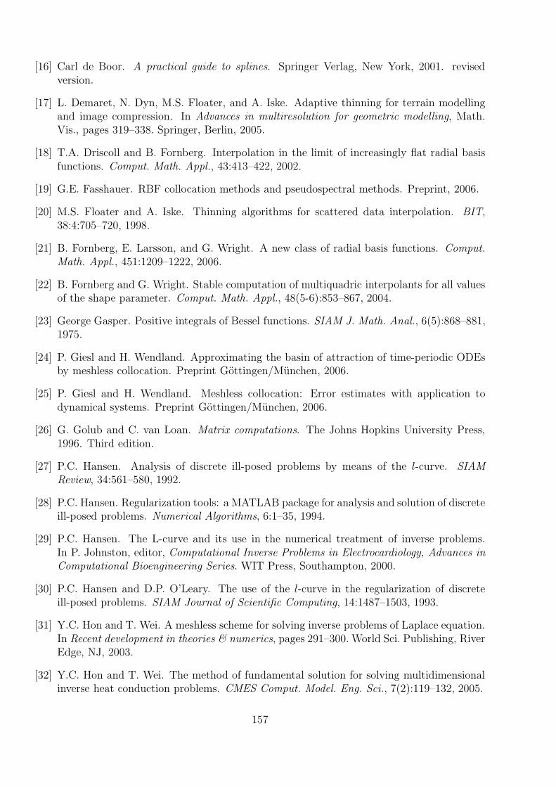
[16] Carl de Boor. A practical guide to splines. Springer Verlag, New York, 2001. revisedversion.

[17] L. Demaret, N. Dyn, M.S. Floater, and A. Iske. Adaptive thinning for terrain modellingand image compression. In Advances in multiresolution for geometric modelling, Math.Vis., pages 319–338. Springer, Berlin, 2005.

[18] T.A. Driscoll and B. Fornberg. Interpolation in the limit of increasingly flat radial basisfunctions. Comput. Math. Appl., 43:413–422, 2002.

[19] G.E. Fasshauer. RBF collocation methods and pseudospectral methods. Preprint, 2006.

[20] M.S. Floater and A. Iske. Thinning algorithms for scattered data interpolation. BIT,38:4:705–720, 1998.

[21] B. Fornberg, E. Larsson, and G. Wright. A new class of radial basis functions. Comput.Math. Appl., 451:1209–1222, 2006.

[22] B. Fornberg and G. Wright. Stable computation of multiquadric interpolants for all valuesof the shape parameter. Comput. Math. Appl., 48(5-6):853–867, 2004.

[23] George Gasper. Positive integrals of Bessel functions. SIAM J. Math. Anal., 6(5):868–881,1975.

[24] P. Giesl and H. Wendland. Approximating the basin of attraction of time-periodic ODEsby meshless collocation. Preprint Gottingen/Munchen, 2006.

[25] P. Giesl and H. Wendland. Meshless collocation: Error estimates with application todynamical systems. Preprint Gottingen/Munchen, 2006.

[26] G. Golub and C. van Loan. Matrix computations. The Johns Hopkins University Press,1996. Third edition.

[27] P.C. Hansen. Analysis of discrete ill-posed problems by means of the l-curve. SIAMReview, 34:561–580, 1992.

[28] P.C. Hansen. Regularization tools: a MATLAB package for analysis and solution of discreteill-posed problems. Numerical Algorithms, 6:1–35, 1994.

[29] P.C. Hansen. The L-curve and its use in the numerical treatment of inverse problems.In P. Johnston, editor, Computational Inverse Problems in Electrocardiology, Advances inComputational Bioengineering Series. WIT Press, Southampton, 2000.

[30] P.C. Hansen and D.P. O’Leary. The use of the l-curve in the regularization of discreteill-posed problems. SIAM Journal of Scientific Computing, 14:1487–1503, 1993.

[31] Y.C. Hon and T. Wei. A meshless scheme for solving inverse problems of Laplace equation.In Recent development in theories & numerics, pages 291–300. World Sci. Publishing, RiverEdge, NJ, 2003.

[32] Y.C. Hon and T. Wei. The method of fundamental solution for solving multidimensionalinverse heat conduction problems. CMES Comput. Model. Eng. Sci., 7(2):119–132, 2005.

157

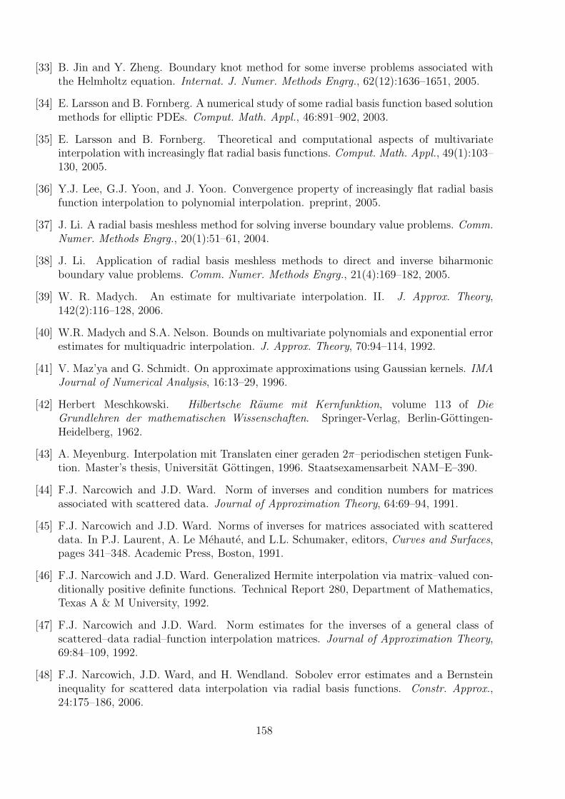
[33] B. Jin and Y. Zheng. Boundary knot method for some inverse problems associated withthe Helmholtz equation. Internat. J. Numer. Methods Engrg., 62(12):1636–1651, 2005.

[34] E. Larsson and B. Fornberg. A numerical study of some radial basis function based solutionmethods for elliptic PDEs. Comput. Math. Appl., 46:891–902, 2003.

[35] E. Larsson and B. Fornberg. Theoretical and computational aspects of multivariateinterpolation with increasingly flat radial basis functions. Comput. Math. Appl., 49(1):103–130, 2005.

[36] Y.J. Lee, G.J. Yoon, and J. Yoon. Convergence property of increasingly flat radial basisfunction interpolation to polynomial interpolation. preprint, 2005.

[37] J. Li. A radial basis meshless method for solving inverse boundary value problems. Comm.Numer. Methods Engrg., 20(1):51–61, 2004.

[38] J. Li. Application of radial basis meshless methods to direct and inverse biharmonicboundary value problems. Comm. Numer. Methods Engrg., 21(4):169–182, 2005.

[39] W. R. Madych. An estimate for multivariate interpolation. II. J. Approx. Theory,142(2):116–128, 2006.

[40] W.R. Madych and S.A. Nelson. Bounds on multivariate polynomials and exponential errorestimates for multiquadric interpolation. J. Approx. Theory, 70:94–114, 1992.

[41] V. Maz’ya and G. Schmidt. On approximate approximations using Gaussian kernels. IMAJournal of Numerical Analysis, 16:13–29, 1996.

[42] Herbert Meschkowski. Hilbertsche Raume mit Kernfunktion, volume 113 of DieGrundlehren der mathematischen Wissenschaften. Springer-Verlag, Berlin-Gottingen-Heidelberg, 1962.

[43] A. Meyenburg. Interpolation mit Translaten einer geraden 2π–periodischen stetigen Funk-tion. Master’s thesis, Universitat Gottingen, 1996. Staatsexamensarbeit NAM–E–390.

[44] F.J. Narcowich and J.D. Ward. Norm of inverses and condition numbers for matricesassociated with scattered data. Journal of Approximation Theory, 64:69–94, 1991.

[45] F.J. Narcowich and J.D. Ward. Norms of inverses for matrices associated with scattereddata. In P.J. Laurent, A. Le Mehaute, and L.L. Schumaker, editors, Curves and Surfaces,pages 341–348. Academic Press, Boston, 1991.

[46] F.J. Narcowich and J.D. Ward. Generalized Hermite interpolation via matrix–valued con-ditionally positive definite functions. Technical Report 280, Department of Mathematics,Texas A & M University, 1992.

[47] F.J. Narcowich and J.D. Ward. Norm estimates for the inverses of a general class ofscattered–data radial–function interpolation matrices. Journal of Approximation Theory,69:84–109, 1992.

[48] F.J. Narcowich, J.D. Ward, and H. Wendland. Sobolev error estimates and a Bernsteininequality for scattered data interpolation via radial basis functions. Constr. Approx.,24:175–186, 2006.

158

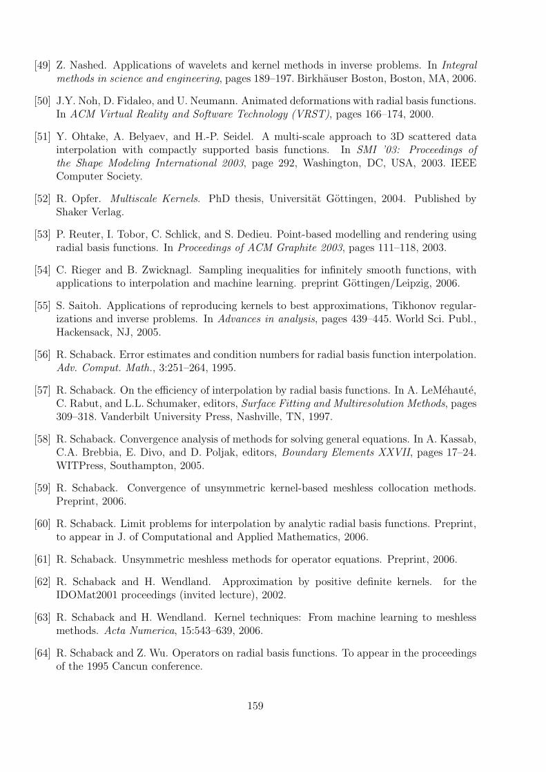
[49] Z. Nashed. Applications of wavelets and kernel methods in inverse problems. In Integralmethods in science and engineering, pages 189–197. Birkhauser Boston, Boston, MA, 2006.

[50] J.Y. Noh, D. Fidaleo, and U. Neumann. Animated deformations with radial basis functions.In ACM Virtual Reality and Software Technology (VRST), pages 166–174, 2000.

[51] Y. Ohtake, A. Belyaev, and H.-P. Seidel. A multi-scale approach to 3D scattered datainterpolation with compactly supported basis functions. In SMI ’03: Proceedings ofthe Shape Modeling International 2003, page 292, Washington, DC, USA, 2003. IEEEComputer Society.

[52] R. Opfer. Multiscale Kernels. PhD thesis, Universitat Gottingen, 2004. Published byShaker Verlag.

[53] P. Reuter, I. Tobor, C. Schlick, and S. Dedieu. Point-based modelling and rendering usingradial basis functions. In Proceedings of ACM Graphite 2003, pages 111–118, 2003.

[54] C. Rieger and B. Zwicknagl. Sampling inequalities for infinitely smooth functions, withapplications to interpolation and machine learning. preprint Gottingen/Leipzig, 2006.

[55] S. Saitoh. Applications of reproducing kernels to best approximations, Tikhonov regular-izations and inverse problems. In Advances in analysis, pages 439–445. World Sci. Publ.,Hackensack, NJ, 2005.

[56] R. Schaback. Error estimates and condition numbers for radial basis function interpolation.Adv. Comput. Math., 3:251–264, 1995.

[57] R. Schaback. On the efficiency of interpolation by radial basis functions. In A. LeMehaute,C. Rabut, and L.L. Schumaker, editors, Surface Fitting and Multiresolution Methods, pages309–318. Vanderbilt University Press, Nashville, TN, 1997.

[58] R. Schaback. Convergence analysis of methods for solving general equations. In A. Kassab,C.A. Brebbia, E. Divo, and D. Poljak, editors, Boundary Elements XXVII, pages 17–24.WITPress, Southampton, 2005.

[59] R. Schaback. Convergence of unsymmetric kernel-based meshless collocation methods.Preprint, 2006.

[60] R. Schaback. Limit problems for interpolation by analytic radial basis functions. Preprint,to appear in J. of Computational and Applied Mathematics, 2006.

[61] R. Schaback. Unsymmetric meshless methods for operator equations. Preprint, 2006.

[62] R. Schaback and H. Wendland. Approximation by positive definite kernels. for theIDOMat2001 proceedings (invited lecture), 2002.

[63] R. Schaback and H. Wendland. Kernel techniques: From machine learning to meshlessmethods. Acta Numerica, 15:543–639, 2006.

[64] R. Schaback and Z. Wu. Operators on radial basis functions. To appear in the proceedingsof the 1995 Cancun conference.

159

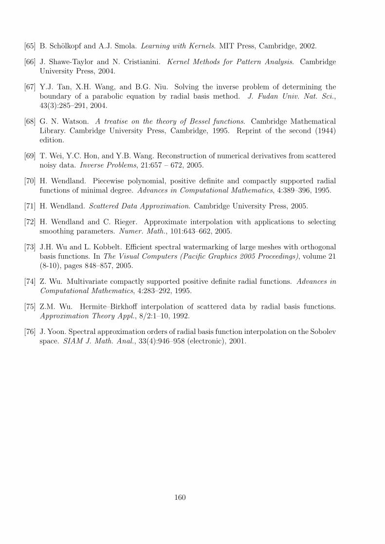
[65] B. Scholkopf and A.J. Smola. Learning with Kernels. MIT Press, Cambridge, 2002.

[66] J. Shawe-Taylor and N. Cristianini. Kernel Methods for Pattern Analysis. CambridgeUniversity Press, 2004.

[67] Y.J. Tan, X.H. Wang, and B.G. Niu. Solving the inverse problem of determining theboundary of a parabolic equation by radial basis method. J. Fudan Univ. Nat. Sci.,43(3):285–291, 2004.

[68] G. N. Watson. A treatise on the theory of Bessel functions. Cambridge MathematicalLibrary. Cambridge University Press, Cambridge, 1995. Reprint of the second (1944)edition.

[69] T. Wei, Y.C. Hon, and Y.B. Wang. Reconstruction of numerical derivatives from scatterednoisy data. Inverse Problems, 21:657 – 672, 2005.

[70] H. Wendland. Piecewise polynomial, positive definite and compactly supported radialfunctions of minimal degree. Advances in Computational Mathematics, 4:389–396, 1995.

[71] H. Wendland. Scattered Data Approximation. Cambridge University Press, 2005.

[72] H. Wendland and C. Rieger. Approximate interpolation with applications to selectingsmoothing parameters. Numer. Math., 101:643–662, 2005.

[73] J.H. Wu and L. Kobbelt. Efficient spectral watermarking of large meshes with orthogonalbasis functions. In The Visual Computers (Pacific Graphics 2005 Proceedings), volume 21(8-10), pages 848–857, 2005.

[74] Z. Wu. Multivariate compactly supported positive definite radial functions. Advances inComputational Mathematics, 4:283–292, 1995.

[75] Z.M. Wu. Hermite–Birkhoff interpolation of scattered data by radial basis functions.Approximation Theory Appl., 8/2:1–10, 1992.

[76] J. Yoon. Spectral approximation orders of radial basis function interpolation on the Sobolevspace. SIAM J. Math. Anal., 33(4):946–958 (electronic), 2001.

160

Index

L-curve method, 33IP k, 35IP–unisolvent, 43

additional conditions, 59analytic RBFs, 63angle, 129approximate approximation, 64autocorrelation function, 90

Banach space, 128band–limited, 98bandlimited functions, 99Beppo–Levi space, 56Bessel function, 151best approximation, 130bounded mapping, 128

cardinal, 26Cauchy-Schwarz inequality, 129closed subspace, 128complete, 128, 132conditional, 34conditionally positive definite, 43conditionally positive definite of order k, 42cone, 89cone axis, 80constraints, 59continuous mapping, 128convergent sequence, 128convex, 79convex combinations, 79convex cone, 5cross-validation, 67

dense, 128derivative approximation, 57distance, 10dual, 128, 134dual , 128dual norm, 9, 134dual space, 9

error analysis, 59error function, 69Euclidean, 129

Euclidean geometry, 129

feature , 3feature space, 3fill distance, 59, 70finite-volume methods, 59flat limit, 62Fourier Inversion Theorem, 144Fourier transform, 142Friedrich’s mollifier, 141functionals, 128

Gamma function, 150Gaussian, 3, 59, 63, 142general interpolation, 58generalized convolution, 6generalized Fourier transform, 148Gram matrix, 131

Hahn–Banach theorem, 75Hankel transform, 98Helmholtz equation, 99hermitian kernel, 1Hilbert space, 132Hilbert–Schmidt, 3

idempotent, 45, 132ill-posed problems, 67index set, 3inner product, 129interior cone condition, 80interpolation conditions , 37inverse problems, 67

kernel, 1, 136kernel function, 36kernel matrix, 4kernel methods, 67

Lagrange, 26Lagrange multipliers, 83Laplace transform, 103Lebesgue function, 74linear hull, 90localized, 75Lyapounov basins, 59

161

machine learning, 67Markov’s inequality, 74Matern kernels, 155Mercer, 3Mercer’s theorem, 5meshless methods, 57mixed interpolation, 58moment conditions, 43, 111monotone operator, 104moving least squares, 74moving least–squares, 81multiquadric, 59, 63multiquadrics, 111

native space, 11, 54, 67noise, 66nonstationary, 64normal equations, 82, 131normalized kernel, 51

operator norm, 128optimization, 30optimization method, 67orbital derivatives, 59order of polynomial, 35orthogonal, 129orthogonal complement, 132oversampling, 73

p, 57partition of unity, 81Plancherel equation, 146Poincare–Friedrichs, 85polyharmonic, 112polyharmonic spline, 62polynomial kernels, 90polynomial splines, 34polynomials, 35positive (semi–) definite,, 4positive definite function, 143power function, 27, 28, 50power kernel, 27Pre–Native Space, 47pre-Hilbert space, 129principal component analysis, 20projection theorem, 132projector, 45, 132

quasi–interpolation, 27

quasi–uniform, 61quasi–uniformity, 84

regularization, 30, 31, 67reproducing kernel, 11reproducing kernel Hilbert space, 12, 136reproduction equation, 8, 136reproduction formula, 36reproduction property, 36Riesz, 135Riesz representation theorem, 134

sampling operator, 74, 79scale parameter, 62scaling, 62seminorm, 129sensitivity to noise, 66separation distance, 60, 118sequence spaces, 130shape factor, 62Shepard approximation, 78, 81singular value decomposition, 20singular values, 20, 31singular-value decomposition, 31smoothness, 61Sobolev kernels, 155Sobolev space, 16spectral condition number, 31stability, 60stabilization, 66stable local polynomial reproduction, 77stationary, 64symmetric kernel, 1

tempered function, 148tempered radial functions, 101tempered test functions, 142thin–plate spline, 34, 112thin-plate spline, 62Tikhonov regularization, 33Tradeoff principle, 118trial functions, 25truncated power, 36truncated singular value decomposition, 32

Uncertainty Principle, 61, 118uniformity constant, 61

warping, 57

162

Weber–Schafheitlin integral, 106Weber-Schafheitlin integral, 155weight function, 81weights, 3

zero sequence, 128

163

Kernel–Based Meshless...

Documents

Transcript of Kernel–Based Meshless...