Int. Conference on Boundary and Interior LayersBAIL 2006

G. Lube, G. Rapin (Eds)c© University of Gottingen, Germany, 2006

On the implementation of the k − ε turbulence model in incompressible

flow solvers based on a finite element discretization

D. Kuzmin and O. Mierka

Institute of Applied Mathematics (LS III), University of DortmundVogelpothsweg 87, D-44227, Dortmund, Germany

kuzmin@math.uni-dortmund.de, omierka@math.uni-dortmund.de

1. Introduction

Turbulence plays an important role in many chemical engineering processes (fluid flow, massand heat transfer, chemical reactions) which are dominated by convective transport. Since thedirect numerical simulation (DNS) of turbulent flows is still prohibitively expensive, eddy vis-cosity models based on the Reynolds Averaged Navier-Stokes (RANS) equations are commonlyemployed in CFD codes. One of the most popular ones is the standard k − ε model which hasbeen in use since the 1970s. However, its practical implementation and, especially, the near-walltreatment has always been some somewhat of a mystery. Algorithmic details and employed‘tricks’ are rarely reported in the literature, so that a novice to this area of CFD research oftenneeds to reinvent the wheel. The numerical implementation of turbulence models involves manyalgorithmic components all of which may have a decisive influence on the quality of simula-tion results. In particular, a positivity-preserving discretization of the troublesome convectiveterms is an important prerequisite for the robustness of the numerical algorithm. This paperpresents a detailed numerical study of the k − ε model implemented in the open-source soft-ware package FeatFlow (http://www.featflow.de) using algebraic flux correction to enforcethe positivity constraint [1, 2]. Emphasis is laid on a new implementation of wall functions,whereby the boundary conditions for k and ε are prescribed in a weak sense. Furthermore,the advantages of Chien’s low-Reynolds number modification are explored. Two representativebenchmark problems are used to evaluate the performance of the proposed algorithms in 3D.

2. Implementation of the k − ε turbulence model

2..1. Mathematical model

In the framework of eddy viscosity models, the hydrodynamic behavior of a turbulent incom-pressible fluid is governed by the RANS equations for the velocity u and pressure p

∂u

∂t+ u · ∇u = −∇p + ∇ ·

(

(ν + νT )[∇u + ∇uT ])

, ∇ · u = 0, (1)

where ν depends only on the physical properties of the fluid, while νT is the turbulent eddyviscosity which is supposed to emulate the effect of unresolved velocity fluctuations u′.

If the standard k − ε model is employed, then νT = Cµk2

ε , where k is the turbulent kineticenergy and ε is the dissipation rate. Hence, the above PDE system is to be complemented bytwo additional convection-diffusion-reaction equations for computation of k and ε

∂k

∂t+ ∇ ·

(

ku − νT

σk∇k

)

= Pk − ε, (2)

∂ε

∂t+ ∇ ·

(

εu− νT

σε∇ε

)

=ε

k(C1Pk − C2ε), (3)

1

where Pk = νT2 |∇u + ∇uT |2 and ε are responsible for production and dissipation of turbulent

kinetic energy, respectively. The default values of the involved empirical constants are as follows:Cµ = 0.09, C1 = 1.44, C2 = 1.92, σk = 1.0, σε = 1.3. Last but not least, equations (1)–(3) areto be endowed with appropriate initial/boundary conditions which will be discussed later.

2..2. Iterative solution strategy

The discretization in space is performed by an unstructured grid finite element method. Theincompressible Navier-Stokes equations are discretized using the nonconforming Q1/Q0 elementpair, whereas standard Q1 elements are employed for k and ε. After an implicit time discretiza-tion by the Crank-Nicolson or backward Euler method, the nodal values of (v, p) and (k, ε) areupdated in a segregated fashion within an outer iteration loop (see below).

For our purposes, it is worthwhile to introduce an auxiliary parameter γ = ǫ/k, which makesit possible to decouple the transport equations (2)–(3) as follows [3]

∂k

∂t+ ∇ ·

(

ku − νT

σk∇k

)

+ γk = Pk, (4)

∂ε

∂t+ ∇ ·

(

εu− νT

σε∇ε

)

+ C2γε = γC1Pk. (5)

This representation provides a positivity-preserving linearization of the sink terms, whereby theparameters νT and γ are evaluated using the solution from the previous outer iteration [2, 4].

The iterative solution process is based on the following hierarchy of nested loops

For n=1,2,... main time-stepping loop tn −→ tn+1

For k=1,2,... outermost coupling loop

• Solve the incompressible Navier-Stokes equations

For l=1,2,... coupling of v and p

For m=1,2,... flux/defect correction

• Solve the transport equations of the k − ε model

For l=1,2,... coupling of k and ε

For m=1,2,... flux/defect correction

At each time step (one n−loop iteration), the governing equations are solved repeatedlywithin the outer k-loop which contains the two subordinate l-loops responsible for the coupling ofvariables within the corresponding subproblem. The embedded m-loops correspond to iterativeflux/defect correction for the involved convection-diffusion operators. Flux limiters of TVD typeare activated in the vicinity of steep gradients, where nonlinear artificial diffusion is required tosuppress nonphysical undershoots and overshoots. In the case of an implicit time discretization,subproblem (4)–(5) leads to a sequence of algebraic systems of the form [1, 2, 4]

A(u(k), γ(l), ν(k)T )∆u(m+1) = r(m), u(m+1) = u(m) + ω∆u(m+1), (6)

where r(m) is the defect vector and the superscripts refer to the loop in which the correspondingvariable is updated. The predicted values k(l+1) and ε(l+1) are used to recompute the lineariza-tion parameter γ(l+1) for the next outer iteration (if any). The associated eddy viscosity νT isbounded from below by a certain fraction of the laminar viscosity 0 < νmin ≤ ν and from above

2

by νmax = lmax

√k, where lmax is the maximum admissible mixing length (the size of the largest

eddies, e.g., the width of the domain). Specifically, we define the limited mixing length l∗ as

l∗ =

Cµk3/2

ε if Cµk3/2 < εlmax

lmax otherwise(7)

and calculate the turbulent eddy viscosity νT from the formula

νT = maxνmin, l∗√

k. (8)

The resulting value of νT is used to update the linearization parameter

γ = Cµk

νT. (9)

The above representation of νT and γ makes it possible to preclude division by zero and obtainbounded nonnegative coefficients without manipulating the actual values of k and ε.

2..2..1 Initial conditions

As a rule, it is rather difficult to devise a reasonable initial guess for a steady-state simulation orproper initial conditions for a dynamic one. If the velocity field is initialized by zero, it takes theflow some time to become fully turbulent. Therefore, we activate the k − ε model at a certaintime t∗ > 0 after the startup. During the ‘laminar’ initial phase (t ≤ t∗), a constant effectiveviscosity ν0 = O(ν) is prescribed. The values to be assigned to k and ε at t = t∗ are uniquelydefined by the choice of ν0 and of the default mixing length l0 ∈ [lmin, lmax] where the thresholdparameter lmin corresponds to the size of the smallest admissible eddies. We have

k0 =

(

ν0

l0

)2

, ε0 = Cµk

3/20

l0at t ≤ t∗. (10)

Alternatively, the initial values of k and ε can be estimated by means of a zero-equation (mix-ing length) turbulence model or computed using an extension of the inflow or wall boundaryconditions (see below) into the interior of the computational domain.

2..2..2 Boundary conditions

At the inflow boundary Γin we prescribe all velocity components and the values of k and ε:

u = g, k = cbc|u|2, ε = Cµk3/2

l0on Γin, (11)

where cbc ∈ [0.003, 0.01] is an empirical constant and |u| =√

u · u is the Euclidean norm of thevelocity. At the outlet Γout, the normal gradients of all variables are set equal to zero, whichcorresponds to the Neumann (‘do-nothing’) boundary condition:

n · [∇u + ∇uT ] = 0, n · ∇k = 0, n · ∇ε = 0 on Γout. (12)

In the finite element framework, these homogeneous boundary conditions imply that the surfaceintegrals resulting from integration by parts in the variational formulation vanish.

At an impervious solid wall Γw, the normal component of the velocity is set equal to zero

n · u = 0 on Γw (13)

whereas tangential slip is permitted in turbulent flow simulations. The practical implementationof the above no-penetration (‘free slip’) boundary condition is nontrivial if the boundary of the

3

computational domain is not aligned with the axes of the Cartesian coordinate system. In thiscase, condition (13) is imposed on a linear combination of several velocity components whereastheir boundary values are unknown. Therefore, standard implementation techniques based ona modification of the corresponding matrix rows cannot be used.

In order to set the normal velocity component equal to zero, we nullify the off-diagonal

entries of the preconditioner A(u(m)) = a(m)ij in the defect correction loop for the momentum

equation [2, 4]. This enables us to compute the boundary values of the vector u explicitly beforesolving a sequence of linear systems for the velocity components:

a(m)ij := 0, ∀j 6= i, u∗

i := u(m)i + r

(m)i /a

(m)ii for xi ∈ Γw. (14)

In the next step, we project the predicted values u∗i onto the tangent vector/plane and

constrain the corresponding entry of the defect vector r(m)i to be zero

u(m)i := u∗

i − (ni · u∗i )ni, r

(m)i := 0 for xi ∈ Γw. (15)

After this manipulation, the corrected values u(m)i act as Dirichlet boundary conditions for the

solution u(m+1)i at the end of the defect correction step. As an alternative to the implementation

technique of predictor-corrector type, the projection can be applied to the residual vector ratherthan to the nodal values of the velocity:

a(m)ij := 0, ∀j 6= i, r

(m)i := r

(m)i − (ni · r(m)

i )ni for xi ∈ Γw. (16)

For Cartesian geometries, the modifications to be performed affect just one velocity component(in the normal direction) as in the case of standard Dirichlet boundary conditions.

2..2..3 Wall functions

To complete the problem statement, we still need to prescribe the tangential stress as well asthe boundary conditions for k and ε on Γw. Note that the equations of the k − ε model areinvalid in the vicinity of the wall where the Reynolds number is rather low and viscous effects aredominant. In order to avoid the need for resolution of strong velocity gradients, wall functionsare typically applied at an internal boundary Γy located at a distance y from the solid wall Γw

n · [∇u + ∇uT ] = −u2τ

νT

u

|u| , k =u2

τ√

Cµ

, ε =u3

τ

κyon Γy, (17)

where κ = 0.41 is the von Karman constant. The above mentioned free-slip condition (13) isalso to be imposed on Γy rather than on Γw. Therefore, u is the tangential velocity which canbe used to compute the friction velocity uτ from the nonlinear equation

|u|uτ

=1

κlog y+ + β (18)

valid in the logarithmic layer, where the local Reynolds number y+ = uτyν is in the range

11.06 ≤ y+ ≤ 300. The empirical constant β equals 5.2 for smooth walls.Strictly speaking, a boundary layer of width y should be removed from the computational

domain Ω. However, it is supposed to be very thin, so that the equations can be solved in thewhole domain Ω with wall functions prescribed on the boundary part Γw rather than on Γy.Since the choice of y is rather arbitrary, it is worthwhile to define the boundary layer width byfixing y+, as proposed in [3, 5]. The implicitly defined y = νy+

uτis assumed to be the point where

the logarithmic layer meets the viscous sublayer so that y+ satisfies (18) as well as the linear

relation y+ = |u|uτ

. The corresponding parameter value y∗+ is given by

y∗+ =1

κlog y∗+ + β ≈ 11.06 on Γy. (19)

4

The use of y∗+ in the wall laws (17)-(19) yields an explicit relation for the friction velocity uτ

which is required to evaluate the tangential stress for the momentum equations [5]

n · [∇u + ∇uT ] = −u∗τ

νT

u

y∗+, where u∗

τ = max

C0.25µ

√k,

|u|y∗+

. (20)

This expression provides a natural boundary condition for the tangential velocity∫

Γw

νT (n · [∇u + ∇uT ] ·w) ds = −∫

Γw

u∗τ

y∗+(u · w) ds. (21)

Due to (17), the boundary value of the turbulent eddy viscosity is proportional to ν

νT = cµk2

ε= κuτy = κy+

∗ ν. (22)

Of course, the above relation is satisfied automatically if the boundary conditions for k andε are implemented in the strong sense as proposed in [2, 4]. However, the use of Dirichletboundary conditions means that the boundary values of k and ε depend solely on the frictionvelocity uτ = |u|

y∗+

which is proportional to the flow velocity at the wall. This results in a one-way

coupling of the boundary conditions which is rather unrealistic. In order to let k and ε ‘float’and influence the momentum equations via (20)-(21), the wall boundary conditions should beimplemented in a weak sense. To this end, let us compute the boundary values of νT fromequation (22) and invoke (17) to retrieve the normal derivatives of k and ε as follows [5]

n · ∇k = −∂k

∂y= 0, n · ∇ε = −∂ε

∂y=

u3τ

κy2=

1

νT

u5τ

y+ν. (23)

These natural boundary conditions are to be plugged into the surface integrals resulting fromintegration by parts in the variational formulation for equations (4) and (5)

∫

Γw

νT

σk(n · ∇k)w ds = 0,

∫

Γw

νT

σε(n · ∇ε)w ds =

∫

Γw

1

σε

u5τ

y+νw ds. (24)

Furthermore, it is commonly assumed that Pk = ε in the wall region, so that the correctboundary value of the production term must be computed from

Pk =u3

τ

κy=

u3τ

νT

|u|y∗+

, where uτ = C0.25µ

√k. (25)

The above implementation of wall functions is largely based on the publication of Grotjans andMenter [5] which should be consulted for further algorithmic details.

2..2..4 Chien’s Low-Reynolds k − ε modification

In the previous section, the implementation of the standard k−ε model was considered, wherebywall functions were prescribed on Γw in order to eliminate the need for a costly integrationto the wall. However, the validity of wall functions is limited to flat-plate boundary layersand developed flow conditions, whereas for accurate simulations of complex flows the modelshould be extended with appropriate Low-Reynolds modifications. Another reason for theirimplementation is that for turbulent flows characterized by rather low Reynolds numbers theremoved region could occupy a significant part of the domain and, therefore, play an importantrole. One of the most commonly used Low-Reynolds modifications is that proposed by Chien [6].It features nice numerical properties and comes with remarkably simple boundary conditions

u = 0, k = 0, ε = 0 on Γw, (26)

5

where the dissipation rate is redefined as ε = ε + 2νk/y2. Furthermore, the following dampingfunctions are introduced to provide a smooth transition from the laminar to the turbulent regime

fµ = 1 − exp(−0.0115y+), f2 = 1 − 0.22 exp

(

k2

6νε

)2

. (27)

The resulting generalization of equations (4)–(5) to the case of low Reynolds numbers reads

∂k

∂t+ ∇ ·

(

ku− νT

σk∇k

)

+

(

γ +2ν

y2

)

k = Pk, νT = Cµfµk2/ε, (28)

∂ε

∂t+ ∇ ·

(

εu− νT

σε∇ε

)

+

(

C2f2γ +2ν

y2exp(−0.5y+)

)

ε = γC1Pk. (29)

The new definition of the turbulent eddy viscosity is in accordance with the DNS results whichreveal that the ratio fµ = νT ε

Cµk2 is not a constant but a function approaching zero at the wall.

Note that the extra sink terms in (28) and (29) have positive coefficients and pose no hazardto positivity of the numerical solution. As before, the linearization parameter γ is recomputedin every outer iteration of the l−loop. The local Reynolds number y+ depending on the friction

velocity uτ (u(k)) is updated at the beginning of the k−loop as follows: uτ =

√

ν ∂vt∂n , where

n is the unit normal to the wall and vt is the tangential velocity at the nearest wall point.Moreover, the update of y+ requires knowing the distance to the wall. In the current imple-mentation, it is computed in a brute-force way as the distance to the nearest midpoint of aboundary edge/face projected onto the uniquely defined normal associated with this edge/face.Alternatively, the computation of the distance can be performed using one of the numerousredistancing/reinitialization algorithms developed in the framework of level set methods.

3. Numerical examples

3..1. Channel flow

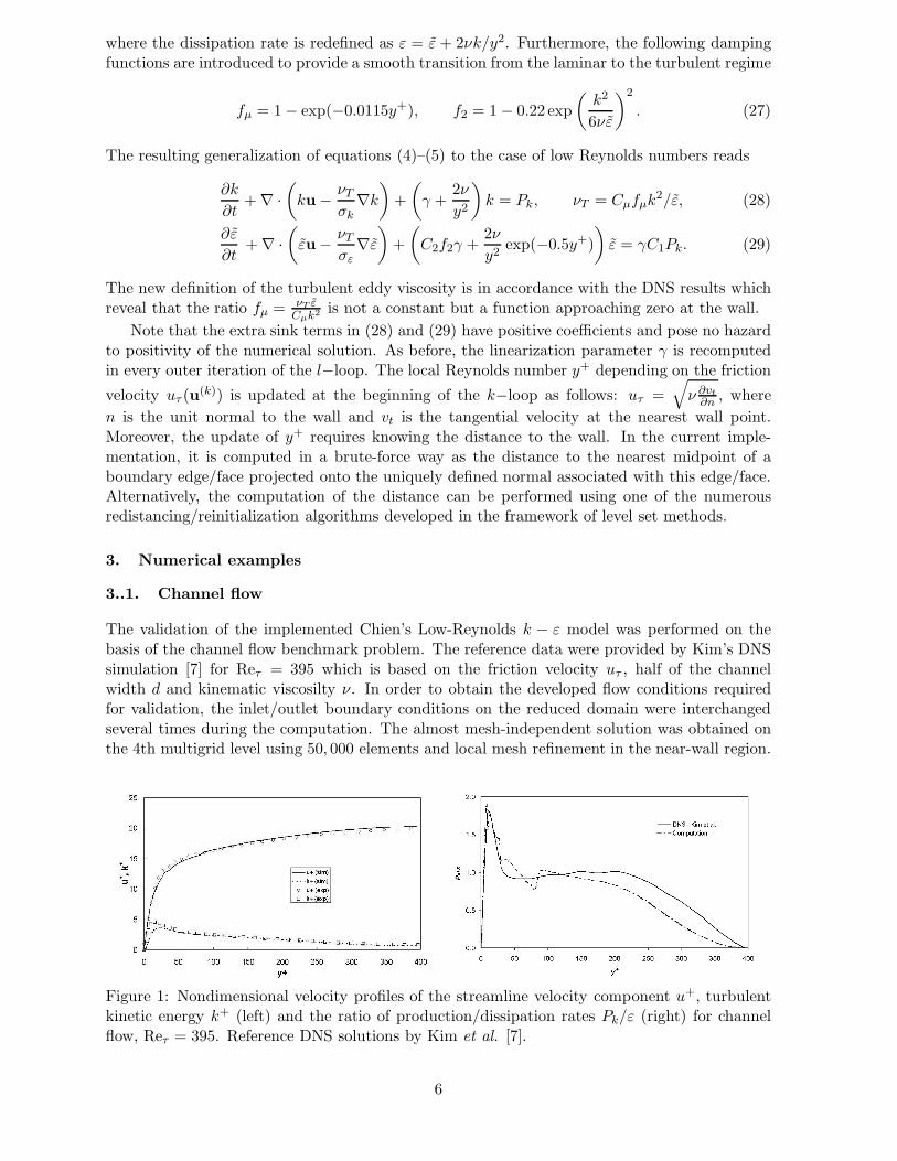
The validation of the implemented Chien’s Low-Reynolds k − ε model was performed on thebasis of the channel flow benchmark problem. The reference data were provided by Kim’s DNSsimulation [7] for Reτ = 395 which is based on the friction velocity uτ , half of the channelwidth d and kinematic viscosilty ν. In order to obtain the developed flow conditions requiredfor validation, the inlet/outlet boundary conditions on the reduced domain were interchangedseveral times during the computation. The almost mesh-independent solution was obtained onthe 4th multigrid level using 50, 000 elements and local mesh refinement in the near-wall region.

Figure 1: Nondimensional velocity profiles of the streamline velocity component u+, turbulentkinetic energy k+ (left) and the ratio of production/dissipation rates Pk/ε (right) for channelflow, Reτ = 395. Reference DNS solutions by Kim et al. [7].

6

The distance from the wall boundary to the nearest interior point corresponds to y+ ≈ 2. Theresulting profiles of the monitored nondimensional quantities (horizontal velocity componentvx, turbulent kinetic energy k as well as the ratio of its production and dissipation rates Pk/ε)displayed in Fig. 1 are in a good agreement with the reference data from [7].

3..2. Backward facing step

The second example deals with a 3D simulation of turbulent incompressible flow past a backwardfacing step using the k − ε model with three different wall boundary treatments (wall functionsimplemented using Dirichlet and Neumann boundary conditions vs. the Low-Reynolds numbermodification based on (26)-(29)). The problem is solved for the Reynolds number Re = 47, 625[8] as defined by the step height H, mean inflow velocity umean and kinematic viscoity ν. All sim-ulations were performed on the same computational mesh consisting of approximately 260, 000elements, see Fig. 2 (top). Local mesh refinement was employed in the vicinity of the walls andbehind the step. The numerical solutions presented in Fig. 2 are in a good agreement with thosepublished in the literature [8]. However, the influence of wall boundary conditions implementedin the strong or weak sense or by means of the Low-Reynolds modification is rather signifi-cant. The recirculation length LR = xr/H predicted by the Low-Reynolds number version andwall functions with Neumann boundary conditions (24) is underestimated (LR ≈ 5.4), whichis also the case for the computational results published in the literature (5.0 < LR < 6.5, see[5, 8, 9]). On the other hand, the implementation of wall functions in the strong sense yieldsLR ≈ 7.1 which matches the experimentally measured recirculation length LR ≈ 7.1, see [10].Unfortunately, this perfect agreement turns out to be a pure coincidence. The numerical solu-tions obtained using different kinds of boundary treatment are compared to one another and toexperimental data [10] in Fig. 3, where 6 different crossplane velocity distributions ux/(ux)max

are plotted at different distances from the step. These profiles indicate that the use of natu-ral boundary conditions (24) yields essentially the same results as the Low-Reynolds numberversion. In either case, the numerical solutions agree well with those presented in [5, 8, 9].

Figure 2: Computational mesh for the backward facing step problem (top) and steady-stateprofiles of the turbulent kinetic energy - ln k (left) and turbulent eddy viscosity - νT (right).From top to bottom: reference solution [7] vs. boundary treatment based on wall functions withDirichlet BC, wall functions with Neumann BC, and Chien’s Low-Reynolds number model.

7

Figure 3: Velocity profiles ux for 6 different distances x/H from the step computed using threedifferent kinds of near-wall treatment for the k − ε model.

References

[1] D. Kuzmin and M. Moller, Algebraic Flux Correction I. Scalar Conservation Laws. In: D.Kuzmin, R. Lohner and S. Turek (eds.) Flux-Corrected Transport: Principles, Algorithms,and Applications. Springer, 2005, 155-206.

[2] S. Turek and D. Kuzmin, Algebraic Flux Correction III. Incompressible Flow Problems.In: D. Kuzmin, R. Lohner and S. Turek (eds.) Flux-Corrected Transport: Principles, Algo-rithms, and Applications. Springer, 2005, 251-296.

[3] A. J. Lew, G. C. Buscaglia and P. M. Carrica, A Note on the Numerical Treatment of thek-epsilon Turbulence Model. Int. J. of Comp. Fluid Dyn. 14 (2001) 201–209.

[4] D. Kuzmin and S. Turek, Multidimensional FEM-TVD Paradigm for Convection-Do-minated Flows. In: Proceedings of the IV European Congress on Computational Methods inApplied Sciences and Engineering (ECCOMAS 2004), Volume II, ISBN 951-39-1869-6.

[5] H. Grotjans and F. Menter, Wall Functions for General Application CFD Codes. ECCO-MAS 98, Proceedings of the 4th European Computational Fluid Dynamics Conference,John Wiley & Sons, 1998, pp. 1112-1117.

[6] K.-Y. Chien, Predictions of Channel and Boundary-Layer Flows with a Low-Reynolds-Number Turbulence Model. AIAA J. 20 (1982) 33–38.

[7] J. Kim, P. Moin and R. D. Moser, Turbulence Statistics in Fully Developed Channel Flowat Low Reynolds Number. J. Fluid Mech. 177 (1987) 133–166.

[8] F. Ilinca, J.-F. Hetu and D. Pelletier, A Unified Finite Element Algorithm for Two-EquationModels of Turbulence. Comp. & Fluids 27-3 (1998) 291–310.

[9] S. Thangam, C. G. Speziale, Turbulent Flow Past a Backward-Facing Step: A CriticalEvaluation of Two-Equation Models, AIAA J. 30-5 (1992), 1314–1320.

[10] J. Kim, Investigation of Separation and Reattachment of Turbulent Shear Layer: Flow overa Backward Facing Step. PhD Thesis, Stanford University, 1978.

8