Noname manuscript No.(will be inserted by the editor)

(α, k)-anonymous data publishing

Raymond Chi-Wing Wong · Jiuyong Li ·Ada Wai-Chee Fu · Ke Wang

the date of receipt and acceptance should be inserted later

Abstract Privacy preservation is an important issue in the release of data for mining

purposes. The k-anonymity model has been introduced for protecting individual iden-

tification. Recent studies show that a more sophisticated model is necessary to protect

the association of individuals to sensitive information. In this paper, we propose an

(α, k)-anonymity model to protect both identifications and relationships to sensitive

information in data. We discuss the properties of (α, k)-anonymity model. We prove

that the optimal (α, k)-anonymity problem is NP-hard. We first present an optimal

global-recoding method for the (α, k)-anonymity problem. Next we propose two scal-

able local-recoding algorithms which are both more scalable and result in less data

Raymond Chi-Wing Wong

Department of Computer Science and Engineering

Hong Kong University of Science and Technology

Jiuyong Li

School of Computer and Information Sciences

University of South Australia

Ada Wai-Chee Fu

Department of Computer Science and Engineering

Chinese university of Hong Kong

Ke wang

Department of Computer Science

Simon Fraser University, Canada

2

distortion. The effectiveness and efficiency are shown by experiments. We also describe

how the model can be extended to more general cases.

Keywords: Privacy, Data Mining, anonymity, privacy preservation, data publishing

1 Introduction

Privacy preservation has become a major issue in many data mining applications.When

a data set is released to other parties for data mining, some privacy-preserving tech-

nique is often required to reduce the possibility of identifying sensitive information

about individuals. This is called the disclosure-control problem [8,28,13] in statistics

and has been studied for many years. Most statistical solutions concern more about

maintaining statistical invariant of data. The data mining community has been study-

ing this problem aiming at building strong privacy-preserving models and designing

efficient optimal and scalable heuristic solutions. The perturbing method [4,2,21] and

the k-anonymity model [23,22] are two major techniques for this goal. The k-anonymity

model has been extensively studied recently because of its relative conceptual simplicity

and effectiveness (e.g. [14,27,10,5,1,20]).

In this paper, we focus on a study on the k-anonymity property [23,22]. The k-

anonymity model assumes a quasi-identifier, which is a set of attributes that may serve

as an identifier in the data set. It is assumed that the dataset is a table and that each

tuple corresponds to an individual. A data set satisfies k-anonymity if there is either

zero or at least k occurrences for any quasi-identifier value. As a result, it is less likely

that any tuple in the released table can be linked to an individual and thus personal

privacy is preserved.

For example, we have a raw medical data set as in Table 1. Attributes job, birth

and postcode1 form the quasi-identifier. Two unique patient records 1 and 2 may be

re-identified easily since their combinations of job, birth and postcode are unique. The

table is generalized as a 2-anonymous table as in Table 2. This table makes the two

patients less likely to be re-identified.

1 We use a simplified postcode scheme in this paper. There are four single digits, representing

states, regions, cities and suburbs. Postcode 4350 indicates state-region-city-suburb.

3

Job Birth Postcode Illness

Cat1 1975 4350 HIV

Cat1 1955 4350 HIV

Cat1 1955 5432 flu

Cat1 1955 5432 fever

Cat2 1975 4350 flu

Cat2 1975 4350 fever

Table 1 Raw Medical Data Set

Job Birth Postcode Illness

Cat1 * 4350 HIV

Cat1 * 4350 HIV

Cat1 1955 5432 flu

Cat1 1955 5432 fever

Cat2 1975 4350 flu

Cat2 1975 4350 fever

Table 2 A 2-anonymous Data Set of Table 1

Job Birth Postcode Illness

* 1975 4350 HIV

* * 4350 HIV

Cat1 1955 5432 flu

Cat1 1955 5432 fever

* * 4350 flu

* 1975 4350 fever

Table 3 An Alternative 2-anonymous Data

Set of Table 1

Job Birth Postcode Illness

* * 4350 HIV

* * 4350 HIV

* * 5432 flu

* * 5432 fever

* * 4350 flu

* * 4350 fever

Table 4 A (0.5, 2)-anonymous Table of Ta-

ble 1 by Full-Domain Generalization

In the literature of privacy preserving, there are two main models. One model is

global recoding [23,16,5,22,14,27,10] while the other is local recoding [24,23,1,20,13,

12]. Assuming a conceptual hierarchy for each attribute, in global recoding, all values

of an attribute come from the same domain level in the hierarchy. For example, all

values in Birth date are in years, or all are in both months and years. One advantage

is that an anonymous view has uniform domains but it may lose more information.

For example, a global recoding of Table 1 may be Table 4 and it suffers from over-

generalization. With local recoding, values may be generalized to different levels in the

domain. For example, Table 2 is a 2-anonymous table by local recoding. In fact one can

say that local recoding is a more general model and global recoding is a special case

of local recoding. Note that, in the example, known values are replaced by unknown

values (*). This is called suppression, which is one special case of generalization, which

is in turn one of the ways of recoding.

4

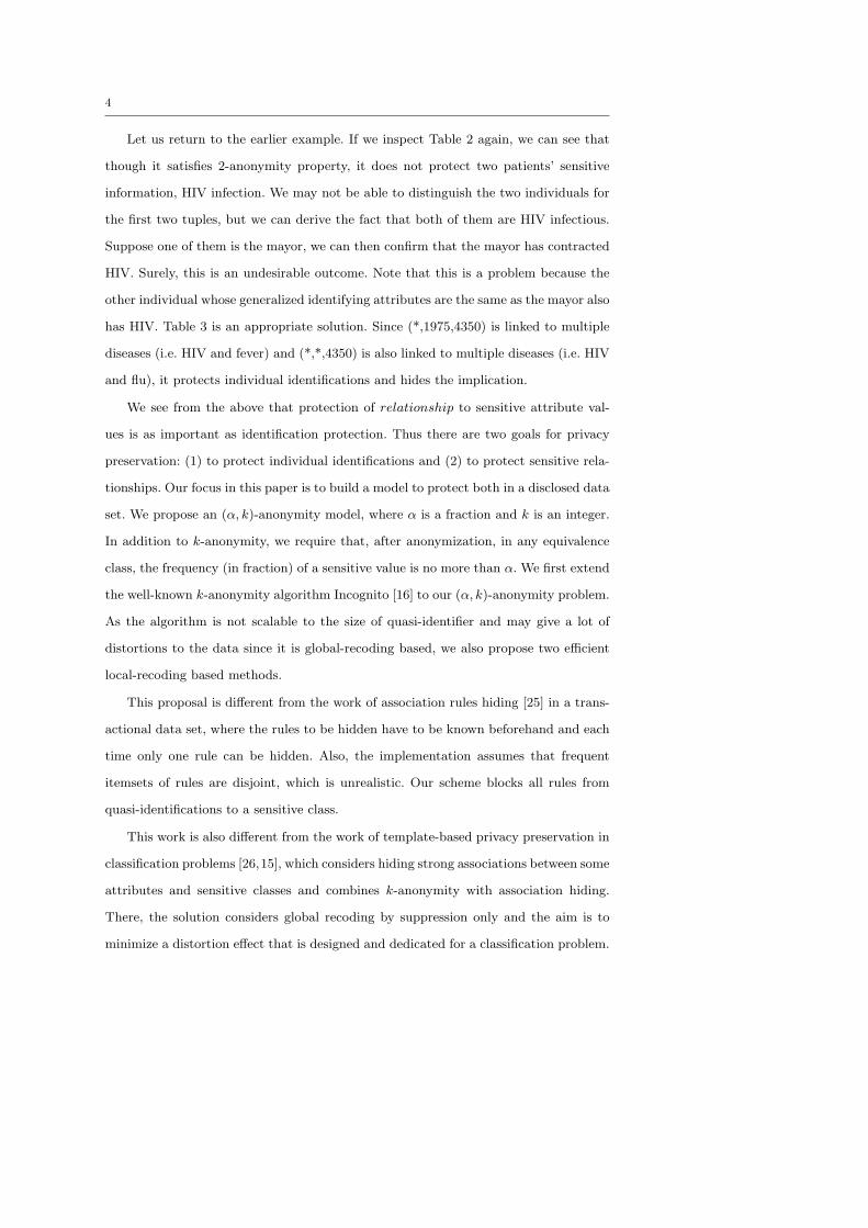
Let us return to the earlier example. If we inspect Table 2 again, we can see that

though it satisfies 2-anonymity property, it does not protect two patients’ sensitive

information, HIV infection. We may not be able to distinguish the two individuals for

the first two tuples, but we can derive the fact that both of them are HIV infectious.

Suppose one of them is the mayor, we can then confirm that the mayor has contracted

HIV. Surely, this is an undesirable outcome. Note that this is a problem because the

other individual whose generalized identifying attributes are the same as the mayor also

has HIV. Table 3 is an appropriate solution. Since (*,1975,4350) is linked to multiple

diseases (i.e. HIV and fever) and (*,*,4350) is also linked to multiple diseases (i.e. HIV

and flu), it protects individual identifications and hides the implication.

We see from the above that protection of relationship to sensitive attribute val-

ues is as important as identification protection. Thus there are two goals for privacy

preservation: (1) to protect individual identifications and (2) to protect sensitive rela-

tionships. Our focus in this paper is to build a model to protect both in a disclosed data

set. We propose an (α, k)-anonymity model, where α is a fraction and k is an integer.

In addition to k-anonymity, we require that, after anonymization, in any equivalence

class, the frequency (in fraction) of a sensitive value is no more than α. We first extend

the well-known k-anonymity algorithm Incognito [16] to our (α, k)-anonymity problem.

As the algorithm is not scalable to the size of quasi-identifier and may give a lot of

distortions to the data since it is global-recoding based, we also propose two efficient

local-recoding based methods.

This proposal is different from the work of association rules hiding [25] in a trans-

actional data set, where the rules to be hidden have to be known beforehand and each

time only one rule can be hidden. Also, the implementation assumes that frequent

itemsets of rules are disjoint, which is unrealistic. Our scheme blocks all rules from

quasi-identifications to a sensitive class.

This work is also different from the work of template-based privacy preservation in

classification problems [26,15], which considers hiding strong associations between some

attributes and sensitive classes and combines k-anonymity with association hiding.

There, the solution considers global recoding by suppression only and the aim is to

minimize a distortion effect that is designed and dedicated for a classification problem.

5

The model defined in this paper is more general in that we allow local recoding and that

we aim at minimizing the distortions of data modifications without any attachment to

a particular data mining method such as classification.

This work is proposed to handle the homogeneity attack as l-diversity model [19]

does. Homogeneity attack is possible when a group of individuals, whose identities are

indistinguishable in a published table, share the same sensitive value. In other words,

an attacker does not need to identify an individual from a group, but can learn his/her

sensitive information. We handle the problem in a different way from l-diversity model.

l-diversity model requires that the sensitive values of every identity undistinguishable

group in a published table has at least l different sensitive values. This gives a general

principle for handling the homogeneity attack, but l-diversity model suffers a major

problem in practice. l-diversity does not specify the protective strength in terms of

probability of leakage. Note that l-diversity does not mean that the probability of

knowing one’s sensitive value is less than 1/l when the distribution of sensitive values

is skewed. Also, it is quite difficult for users to set parameter l. In contrast, α in our

model is a probabilistic parameter and is intuitive to set. Furthermore, the proposed

algorithm in [19] is based on a global-recoding algorithm Incognito, which may generate

more distortion compared to a local recoding approach. We propose two local recoding

algorithms which can give low information loss.

It is worth mentioning other works [18,29,30,7] which are also related to us although

they are different from us. [18] proposed a privacy model called t-closeness. With this

model, the distribution in each A-group in T ∗ with respect to the sensitive attribute

is roughly equal to the distribution of the entire table T ∗. The difference between the

distribution in each A-group and the distribution of the entire table should be bounded

with a parameter t. However, similar to l-diversity, it is difficult for the users to set

parameter t since parameter t is not intuitive. [29] proposed a personalized privacy

model such that each individual can provide his/her preference on the protection of

his/her sensitive value. The above works study the problem for a one-time publication.

[30,7] proposed the problems for multiple-time publications. In this paper, we focus on

the one-time publication.

6

We propose to handle issues of k-anonymity with protection of some sensitive val-

ues. This is based on the fact that we could not protect too many sensitive values in

a data set. If we do, a published data set may be hardly useful because of too many

distortions have been done to the data set. Practically, not all sensitive information is

considered as privacy. For example, people care more about depression than virus in-

fection. We consider our proposed method as a practical enhancement of k-anonymity

with the consideration of the utility of published data.

Our Contributions:

– We propose a simple and effective model to protect both identifications and sensi-

tive associations in a disclosed data set. The model extends the k-anonymity model

to the (α, k)-anonymity model to limit the confidence of the implications from the

quasi-identifier to a sensitive value (attribute) to within α in order to protect the

sensitive information from being inferred by strong implications. We prove that the

optimal (α, k)-anonymity by local recoding is NP-hard.

– We extend Incognito[16], a global-recoding algorithm for the k-anonymity problem,

to solve this problem for (α, k)-anonymity. We also propose two local-recoding

algorithms, which are scalable and generate less distortion. In our experiment, we

show that, on average, the two local-recoding based algorithms performs about 4

times faster and gives about 3 times less distortions of the data set compared with

the extended Incognito algorithm.

2 Problem Definition

We assume that each attribute has a corresponding conceptual hierarchy or taxonomy.

A lower level domain in the hierarchy provides more details than a higher level domain.

For example, birth date in D/M/Y (e.g. 15/Mar/1970) is a lower level domain and

birth date in Y (e.g. 1970) is a higher level domain. We assume such hierarchies for

numerical attributes too. In particular, we have a hierarchical structure defined with

{value, interval, *}, where value is the raw numerical data, interval is the range of the

raw data and * is a symbol representing any values. Intervals can be determined by

users or a machine learning algorithm [9]. In a hierarchy domains with fewer values

7

are more general than domains with more values for an attribute. The most general

domain contains only one value. For example, 10-year interval level in birth domain

is more general than one-year level. The most general level of birth domain contains

value unknown (e.g. *). Generalization replaces lower level domain values with higher

level domain values. For example, birth D/M/Y is replaced by M/Y.

Let D be a data set or a table. A record of D is a tuple or a row. An attribute

defines all the possible values in a column. For a data set to be disclosed, any identifier

column (e.g. secure id and passport number) is definitely removed. However, some

attribute combinations after this removal may still identify some individuals.

Definition 1 (Quasi-identifier) A quasi-identifier is a minimum set of attributes of

D that may serve as identifications for some tuples in D.

For example, domain expert may decide that the attribute set {Job, Birth, Post-

code} in Tables 1- 4 is a quasi-identifier. The first goal of privacy preserving is to

remove all possible identifications in a disclosed table (according to the quasi-identifer)

so that individuals are not identifiable. We define an important concept, equivalence

class, which is fundamental to our (α, k)-anonymity model.

Definition 2 (Equivalence Class) Let Q be an attribute set. An equivalence class

of a table with respect to attribute set Q is a collection of all tuples in the table

containing identical values for attribute set Q.

For example, tuples 1 and 2 in Table 2 form an equivalence class with respect

to attribute set {Job, Birth, Postcode}. The size of an equivalence class indicates

the strength of identification protection of individuals in the equivalent class. If the

number of tuples in an equivalence class is greater, it will be more difficult to re-identify

individual.

Definition 3 (k-Anonymity Property) Let Q be an attribute set. A data set D is

k-anonymous with respect to attribute set Q if the size of every equivalence class with

respect to attribute set Q is k or more.

The k-anonymity model requires that every value set for the quasi-identifier at-

tribute set has a frequency of zero or at least k. For example, Table 1 does not satisfy

8

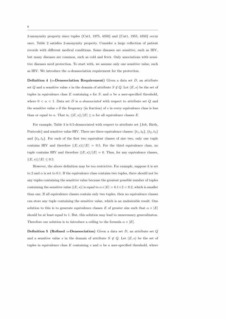
2-anonymity property since tuples {Cat1, 1975, 4350} and {Cat1, 1955, 4350} occur

once. Table 2 satisfies 2-anonymity property. Consider a large collection of patient

records with different medical conditions. Some diseases are sensitive, such as HIV,

but many diseases are common, such as cold and fever. Only associations with sensi-

tive diseases need protection. To start with, we assume only one sensitive value, such

as HIV. We introduce the α-deassociation requirement for the protection.

Definition 4 (α-Deassociation Requirement) Given a data set D, an attribute

set Q and a sensitive value s in the domain of attribute S 6∈ Q. Let (E, s) be the set of

tuples in equivalence class E containing s for S. and α be a user-specified threshold,

where 0 < α < 1. Data set D is α-deassociated with respect to attribute set Q and

the sensitive value s if the frequency (in fraction) of s in every equivalence class is less

than or equal to α. That is, |(E, s)|/|E| ≤ α for all equivalence classes E.

For example, Table 3 is 0.5-deassociated with respect to attribute set {Job, Birth,

Postcode} and sensitive value HIV. There are three equivalence classes: {t1, t6}, {t2, t5}and {t3, t4}. For each of the first two equivalent classes of size two, only one tuple

contains HIV and therefore |(E, s)|/|E| = 0.5. For the third equivalence class, no

tuple contains HIV and therefore |(E, s)|/|E| = 0. Thus, for any equivalence classes,

|(E, s)|/|E| ≤ 0.5.

However, the above definition may be too restrictive. For example, suppose k is set

to 2 and α is set to 0.1. If the equivalence class contains two tuples, there should not be

any tuples containing the sensitive value because the greatest possible number of tuples

containing the sensitive value |(E, s)| is equal to α×|E| = 0.1×2 = 0.2, which is smaller

than one. If all equivalence classes contain only two tuples, then no equivalence classes

can store any tuple containing the sensitive value, which is an undesirable result. One

solution to this is to generate equivalence classes E of greater size such that α × |E|should be at least equal to 1. But, this solution may lead to unnecessary generalizaton.

Therefore our solution is to introduce a ceiling to the formula α× |E|.

Definition 5 (Refined α-Deassociation) Given a data set D, an attribute set Q

and a sensitive value s in the domain of attribute S 6∈ Q. Let (E, s) be the set of

tuples in equivalence class E containing s and α be a user-specified threshold, where

9

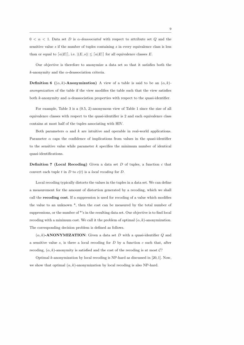
0 < α < 1. Data set D is α-deassociated with respect to attribute set Q and the

sensitive value s if the number of tuples containing s in every equivalence class is less

than or equal to dα|E|e, i.e. |(E, s)| ≤ dα|E|e for all equivalence classes E.

Our objective is therefore to anonymize a data set so that it satisfies both the

k-anonymity and the α-deassociation criteria.

Definition 6 ((α, k)-Anonymization) A view of a table is said to be an (α, k)-

anonymization of the table if the view modifies the table such that the view satisfies

both k-anonymity and α-deassociation properties with respect to the quasi-identifier.

For example, Table 3 is a (0.5, 2)-anonymous view of Table 1 since the size of all

equivalence classes with respect to the quasi-identifier is 2 and each equivalence class

contains at most half of the tuples associating with HIV.

Both parameters α and k are intuitive and operable in real-world applications.

Parameter α caps the confidence of implications from values in the quasi-identifier

to the sensitive value while parameter k specifies the minimum number of identical

quasi-identifications.

Definition 7 (Local Recoding) Given a data set D of tuples, a function c that

convert each tuple t in D to c(t) is a local recoding for D.

Local recoding typically distorts the values in the tuples in a data set. We can define

a measurement for the amount of distortion generated by a recoding, which we shall

call the recoding cost. If a suppression is used for recoding of a value which modifies

the value to an unknown *, then the cost can be measured by the total number of

suppressions, or the number of *’s in the resulting data set. Our objective is to find local

recoding with a minimum cost. We call it the problem of optimal (α, k)-anonymization.

The corresponding decision problem is defined as follows.

(α, k)-ANONYMIZATION: Given a data set D with a quasi-identifier Q and

a sensitive value s, is there a local recoding for D by a function c such that, after

recoding, (α, k)-anonymity is satisfied and the cost of the recoding is at most C?Optimal k-anonymization by local recoding is NP-hard as discussed in [20,1]. Now,

we show that optimal (α, k)-anonymization by local recoding is also NP-hard.

10

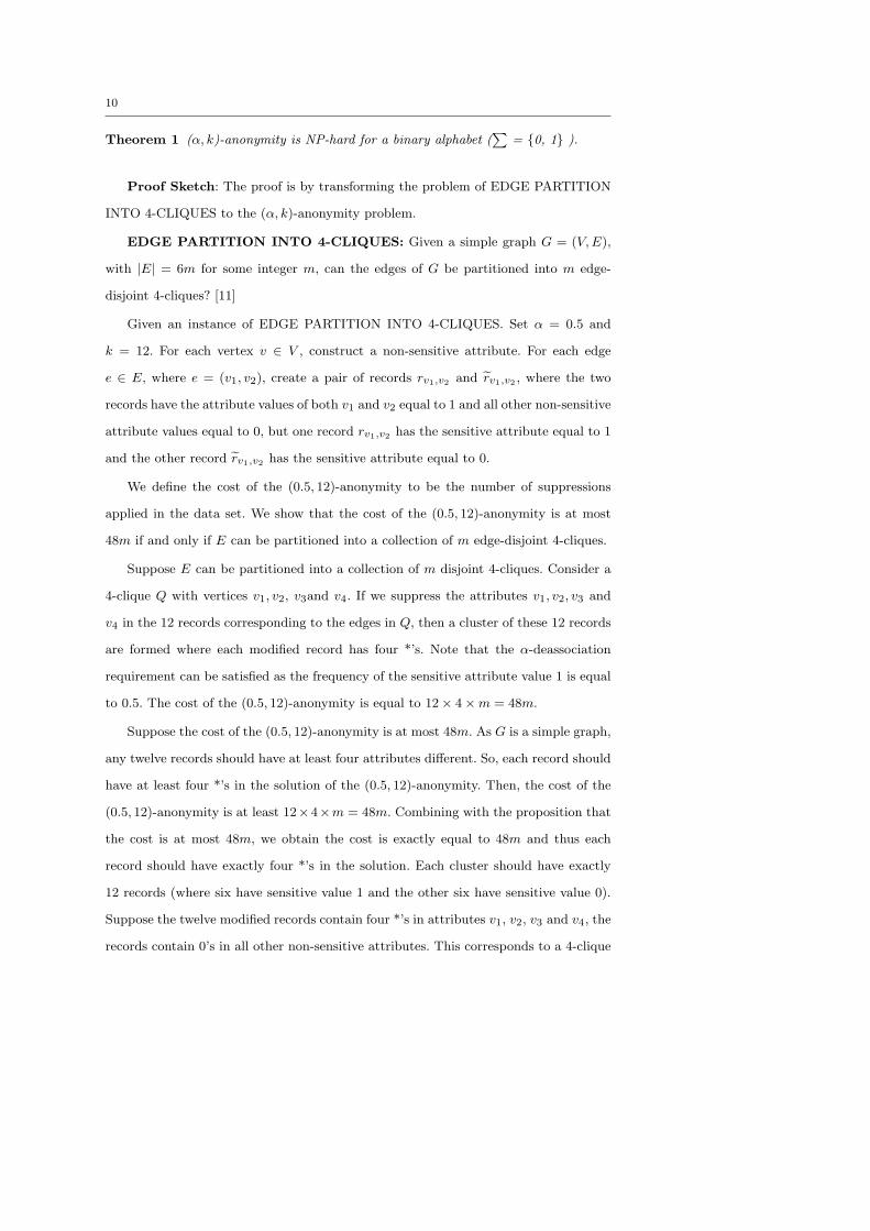
Theorem 1 (α, k)-anonymity is NP-hard for a binary alphabet (∑

= {0, 1} ).

Proof Sketch: The proof is by transforming the problem of EDGE PARTITION

INTO 4-CLIQUES to the (α, k)-anonymity problem.

EDGE PARTITION INTO 4-CLIQUES: Given a simple graph G = (V, E),

with |E| = 6m for some integer m, can the edges of G be partitioned into m edge-

disjoint 4-cliques? [11]

Given an instance of EDGE PARTITION INTO 4-CLIQUES. Set α = 0.5 and

k = 12. For each vertex v ∈ V , construct a non-sensitive attribute. For each edge

e ∈ E, where e = (v1, v2), create a pair of records rv1,v2 and r̃v1,v2 , where the two

records have the attribute values of both v1 and v2 equal to 1 and all other non-sensitive

attribute values equal to 0, but one record rv1,v2 has the sensitive attribute equal to 1

and the other record r̃v1,v2 has the sensitive attribute equal to 0.

We define the cost of the (0.5, 12)-anonymity to be the number of suppressions

applied in the data set. We show that the cost of the (0.5, 12)-anonymity is at most

48m if and only if E can be partitioned into a collection of m edge-disjoint 4-cliques.

Suppose E can be partitioned into a collection of m disjoint 4-cliques. Consider a

4-clique Q with vertices v1, v2, v3and v4. If we suppress the attributes v1, v2, v3 and

v4 in the 12 records corresponding to the edges in Q, then a cluster of these 12 records

are formed where each modified record has four *’s. Note that the α-deassociation

requirement can be satisfied as the frequency of the sensitive attribute value 1 is equal

to 0.5. The cost of the (0.5, 12)-anonymity is equal to 12× 4×m = 48m.

Suppose the cost of the (0.5, 12)-anonymity is at most 48m. As G is a simple graph,

any twelve records should have at least four attributes different. So, each record should

have at least four *’s in the solution of the (0.5, 12)-anonymity. Then, the cost of the

(0.5, 12)-anonymity is at least 12×4×m = 48m. Combining with the proposition that

the cost is at most 48m, we obtain the cost is exactly equal to 48m and thus each

record should have exactly four *’s in the solution. Each cluster should have exactly

12 records (where six have sensitive value 1 and the other six have sensitive value 0).

Suppose the twelve modified records contain four *’s in attributes v1, v2, v3 and v4, the

records contain 0’s in all other non-sensitive attributes. This corresponds to a 4-clique

11

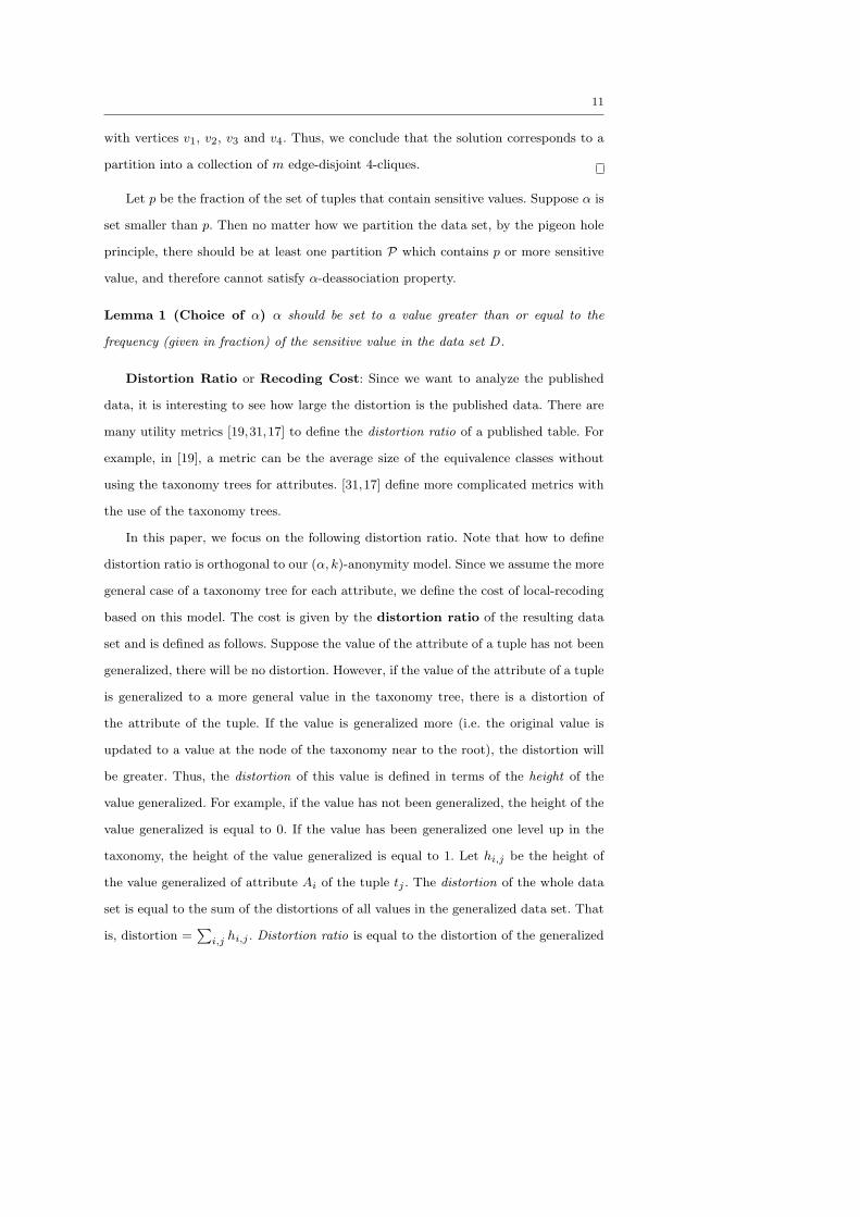
with vertices v1, v2, v3 and v4. Thus, we conclude that the solution corresponds to a

partition into a collection of m edge-disjoint 4-cliques.

Let p be the fraction of the set of tuples that contain sensitive values. Suppose α is

set smaller than p. Then no matter how we partition the data set, by the pigeon hole

principle, there should be at least one partition P which contains p or more sensitive

value, and therefore cannot satisfy α-deassociation property.

Lemma 1 (Choice of α) α should be set to a value greater than or equal to the

frequency (given in fraction) of the sensitive value in the data set D.

Distortion Ratio or Recoding Cost: Since we want to analyze the published

data, it is interesting to see how large the distortion is the published data. There are

many utility metrics [19,31,17] to define the distortion ratio of a published table. For

example, in [19], a metric can be the average size of the equivalence classes without

using the taxonomy trees for attributes. [31,17] define more complicated metrics with

the use of the taxonomy trees.

In this paper, we focus on the following distortion ratio. Note that how to define

distortion ratio is orthogonal to our (α, k)-anonymity model. Since we assume the more

general case of a taxonomy tree for each attribute, we define the cost of local-recoding

based on this model. The cost is given by the distortion ratio of the resulting data

set and is defined as follows. Suppose the value of the attribute of a tuple has not been

generalized, there will be no distortion. However, if the value of the attribute of a tuple

is generalized to a more general value in the taxonomy tree, there is a distortion of

the attribute of the tuple. If the value is generalized more (i.e. the original value is

updated to a value at the node of the taxonomy near to the root), the distortion will

be greater. Thus, the distortion of this value is defined in terms of the height of the

value generalized. For example, if the value has not been generalized, the height of the

value generalized is equal to 0. If the value has been generalized one level up in the

taxonomy, the height of the value generalized is equal to 1. Let hi,j be the height of

the value generalized of attribute Ai of the tuple tj . The distortion of the whole data

set is equal to the sum of the distortions of all values in the generalized data set. That

is, distortion =∑

i,j hi,j . Distortion ratio is equal to the distortion of the generalized

12

Gender Birth Postcode Sens

male May 1965 4351 n

male Jun 1965 4351 c

male Jul 1965 4361 n

male Aug 1965 4362 n

Table 5 A Data Set

data set divided by the distortion of the fully generalized data set, where the fully

generalized data set is one with all values of the attributes are generalized to the root

of the taxonomy.

3 Global-Recoding

In this section, we extend an existing global-recoding based algorithm called Incognito

[16] for the (α, k)-anonymous model. Incognito algorithm [16] is an optimal algorithm

for the k-anonymity problem. It has also been used in [19] for the l-diversity problem.

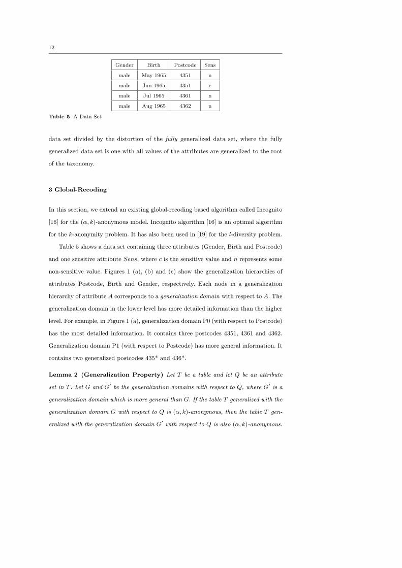
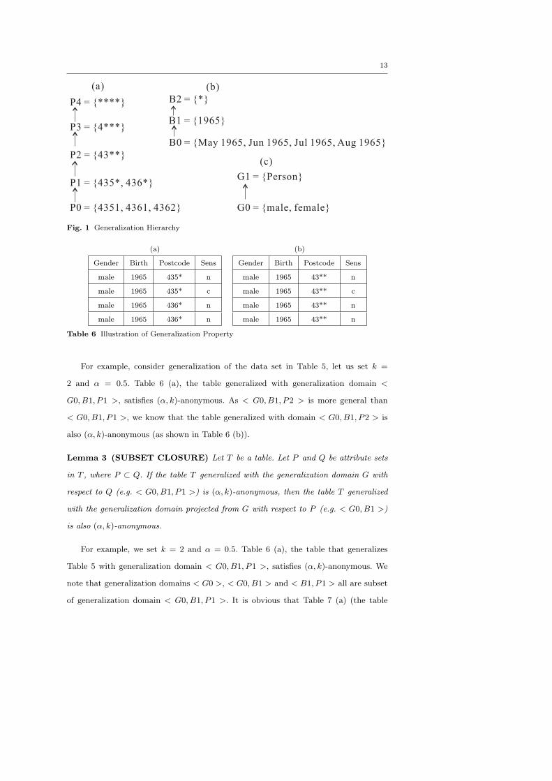
Table 5 shows a data set containing three attributes (Gender, Birth and Postcode)

and one sensitive attribute Sens, where c is the sensitive value and n represents some

non-sensitive value. Figures 1 (a), (b) and (c) show the generalization hierarchies of

attributes Postcode, Birth and Gender, respectively. Each node in a generalization

hierarchy of attribute A corresponds to a generalization domain with respect to A. The

generalization domain in the lower level has more detailed information than the higher

level. For example, in Figure 1 (a), generalization domain P0 (with respect to Postcode)

has the most detailed information. It contains three postcodes 4351, 4361 and 4362.

Generalization domain P1 (with respect to Postcode) has more general information. It

contains two generalized postcodes 435* and 436*.

Lemma 2 (Generalization Property) Let T be a table and let Q be an attribute

set in T . Let G and G′ be the generalization domains with respect to Q, where G′ is a

generalization domain which is more general than G. If the table T generalized with the

generalization domain G with respect to Q is (α, k)-anonymous, then the table T gen-

eralized with the generalization domain G′ with respect to Q is also (α, k)-anonymous.

13

P4 = {****}

P3 = {4***}

P2 = {43**}

P1 = {435*, 436*}

P0 = {4351, 4361, 4362}

B2 = {*}

B1 = {1965}

B0 = {May 1965, Jun 1965, Jul 1965, Aug 1965}

G0 = {male, female}

G1 = {Person}

(a) (b)

(c)

Fig. 1 Generalization Hierarchy

(a) (b)

Gender Birth Postcode Sens

male 1965 435* n

male 1965 435* c

male 1965 436* n

male 1965 436* n

Gender Birth Postcode Sens

male 1965 43** n

male 1965 43** c

male 1965 43** n

male 1965 43** n

Table 6 Illustration of Generalization Property

For example, consider generalization of the data set in Table 5, let us set k =

2 and α = 0.5. Table 6 (a), the table generalized with generalization domain <

G0, B1, P1 >, satisfies (α, k)-anonymous. As < G0, B1, P2 > is more general than

< G0, B1, P1 >, we know that the table generalized with domain < G0, B1, P2 > is

also (α, k)-anonymous (as shown in Table 6 (b)).

Lemma 3 (SUBSET CLOSURE) Let T be a table. Let P and Q be attribute sets

in T , where P ⊂ Q. If the table T generalized with the generalization domain G with

respect to Q (e.g. < G0, B1, P1 >) is (α, k)-anonymous, then the table T generalized

with the generalization domain projected from G with respect to P (e.g. < G0, B1 >)

is also (α, k)-anonymous.

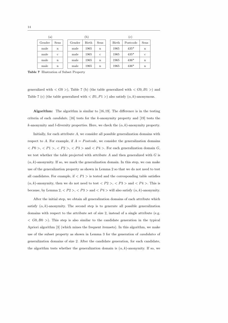
For example, we set k = 2 and α = 0.5. Table 6 (a), the table that generalizes

Table 5 with generalization domain < G0, B1, P1 >, satisfies (α, k)-anonymous. We

note that generalization domains < G0 >, < G0, B1 > and < B1, P1 > all are subset

of generalization domain < G0, B1, P1 >. It is obvious that Table 7 (a) (the table

14

(a) (b) (c)

Gender Sens

male n

male c

male n

male n

Gender Birth Sens

male 1965 n

male 1965 c

male 1965 n

male 1965 n

Birth Postcode Sens

1965 435* n

1965 435* c

1965 436* n

1965 436* n

Table 7 Illustration of Subset Property

generalized with < G0 >), Table 7 (b) (the table generalized with < G0, B1 >) and

Table 7 (c) (the table generalized with < B1, P1 >) also satisfy (α, k)-anonymous.

Algorithm: The algorithm is similar to [16,19]. The difference is in the testing

criteria of each candidate. [16] tests for the k-anonymity property and [19] tests the

k-anonymity and l-diversity properties. Here, we check the (α, k)-anonymity property.

Initially, for each attribute A, we consider all possible generalization domains with

respect to A. For example, if A = Postcode, we consider the generalization domains

< P0 >, < P1 >, < P2 >, < P3 > and < P4 >. For each generalization domain G,

we test whether the table projected with attribute A and then generalized with G is

(α, k)-anonymity. If so, we mark the generalization domain. In this step, we can make

use of the generalization property as shown in Lemma 2 so that we do not need to test

all candidates. For example, if < P1 > is tested and the corresponding table satisfies

(α, k)-anonymity, then we do not need to test < P2 >, < P3 > and < P4 >. This is

because, by Lemma 2, < P2 >, < P3 > and < P4 > will also satisfy (α, k)-anonymity.

After the initial step, we obtain all generalization domains of each attribute which

satisfy (α, k)-anonymity. The second step is to generate all possible generalization

domains with respect to the attribute set of size 2, instead of a single attribute (e.g.

< G0, B0 >). This step is also similar to the candidate generation in the typical

Apriori algorithm [3] (which mines the frequent itemsets). In this algorithm, we make

use of the subset property as shown in Lemma 3 for the generation of candidates of

generalization domains of size 2. After the candidate generation, for each candidate,

the algorithm tests whether the generalization domain is (α, k)-anonymity. If so, we

15

mark the generalization domain. Similar to the first step, the second step can also make

use of the generalization property for pruning.

The step repeats until all generalization domains of size |Q| is reached, where Q

is the quasi-identifier. Then, among all these domains of size |Q|, we choose one with

the minimum distortion as the final generalization domain G of the table. Next G is

applied to the given table to obtain an (α, k)-anonymous table, which is our output.

4 Local-Recoding

The extended Incognito algorithm is an exhaustive global recoding algorithm which is

not scalable and may generate excessive distortions to the data set. Here we propose

two scalable heuristic algorithms called Progressive Local Recoding (Section 4.1) and

Top-Down Approach (Section 4.2) for (α, k)-anonymization by local recoding.

4.1 Progressive Local Recoding

In this section, we present a scalable progressive local-recoding method for (α, k)-

anonymization. The first local-recoding method we propose is progressive because we

shall repeatedly pick an attribute and generalize the data set by going one level up its

taxonomy. The choice of the next attribute to be generalized is based on a heuristic

criterion. This process repeats until the table satisfies (α, k)-anonymity. In the process

of the generalization, some tuples will satisfy (α, k)-anonymity earlier than others. We

do not repeatedly generalize the chosen attribute of all tuples. Instead, we will remove

some tuples satisfying (α, k)-anonymity from the data set being processed in order to

avoid further distortion to these tuples, and to advance to a smaller data set in the

processing. In our method, there are two kinds of removal. The first removal is called

α-deassociated removal while the second removal is called further removal.

Criteria of Choosing Attribute - Entropy: A simple heuristic of choosing the

next attribute for generalization is choosing one with the most values. Among those

attributes with a similar number of values, one whose values are more evenly distributed

is chosen. It is intuitive that a generalization domain with more values is typically at

16

a lower level in the taxonomy and it is reasonable to move up the taxonomy. If the

values are skewed, then the attribute is close to a generalized state since most values

are already identical. Therefore we can gain more in terms of uniformity by picking an

attribute with values that are more evenly distributed.

Interestingly, entropy is a measurement that can capture both of the above criteria.

Let E be the entropy of an attribute Ai. E =∑∀v∈Ai

[−P (v) log2 P (v)], where P (v) is

the probability of value v occurring in attribute Ai. For example, for an attribute with

ten evenly distributed values, E = 10× (−(1/10) log2(1/10)) = 3.32. For an attribute

with two evenly distributed values, E = 2 × (−(1/2) log2(1/2)) = 1. For an attribute

with two unevenly distributed values, one has the frequency of 0.8 and the other has

the frequency of 0.2. E = −(4/5) log2(4/5) − (1/5) log2(1/5) = 0.722. We choose the

attribute with the highest entropy among all attributes to be generalized first.

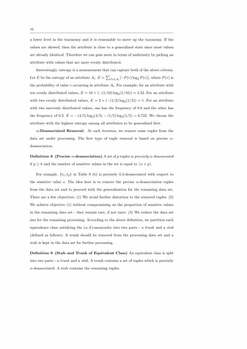
α-Deassociated Removal: At each iteration, we remove some tuples from the

data set under processing. The first type of tuple removal is based on precise α-

deassociation.

Definition 8 (Precise α-deassociation) A set of p tuples is precisely α-deassociated

if p ≥ k and the number of sensitive values in the set is equal to dα× pe.

For example, {t1, t2} in Table 9 (b) is precisely 0.5-deassociated with respect to

the sensitive value s. The idea here is to remove the precise α-deassociation tuples

from the data set and to proceed with the generalization for the remaining data set.

There are a few objectives: (1) We avoid further distortion to the removed tuples. (2)

We achieve objective (1) without compromising on the proportion of sensitive values

in the remaining data set - they remain rare, if not rarer. (3) We reduce the data set

size for the remaining processing. According to the above definition, we partition each

equivalence class satisfying the (α, k)-anonymity into two parts - a trunk and a stub

(defined as follows). A trunk should be removed from the processing data set and a

stub is kept in the data set for further processing.

Definition 9 (Stub and Trunk of Equivalent Class) An equivalent class is split

into two parts - a trunk and a stub. A trunk contains a set of tuples which is precisely

α-deassociated. A stub contains the remaining tuples.

17

(a) (b)

Gender Birth Postcode Sens

male May 1965 4351 n

male Jun 1965 4351 c

male Jul 1965 4351 n

male Aug 1965 4352 n

Gender Birth Postcode Sens

male 1965 435* n

male 1965 435* c

male 1965 435* n

male 1965 435* n

Table 8 A Full-Domain Generalization Solution

(a) (b)

Gender Birth Postcode Sens

male May 1965 4351 n

male Jun 1965 4351 c

male Jul 1965 4351 n

male Aug 1965 4352 n

Gender Birth Postcode Sens

male 1965 4351 n

male 1965 4351 c

male 1965 4351 n

male 1965 4352 n

(c)

Gender Birth Postcode Sens

male 1965 4351 n

male 1965 4351 c

male 1965 435* n

male 1965 435* n

Table 9 An Illustration of Our Approach

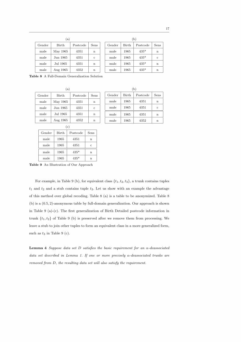
For example, in Table 9 (b), for equivalent class {t1, t2, t3}, a trunk contains tuples

t1 and t2 and a stub contains tuple t3. Let us show with an example the advantage

of this method over global recoding. Table 8 (a) is a table to be anonymized. Table 8

(b) is a (0.5, 2)-anonymous table by full-domain generalization. Our approach is shown

in Table 9 (a)-(c). The first generalization of Birth Detailed postcode information in

trunk {t1, t2} of Table 9 (b) is preserved after we remove them from processing. We

leave a stub to join other tuples to form an equivalent class in a more generalized form,

such as t3 in Table 9 (c).

Lemma 4 Suppose data set D satisfies the basic requirement for an α-deassociated

data set described in Lemma 1. If one or more precisely α-deassociated trunks are

removed from D, the resulting data set will also satisfy the requirement.

18

The proof of this lemma is trivial and is omitted here.

This lemma enables us to separate precisely α-deassociated trunks from a data set

knowing that the remaining data set can still be α-deassociated.

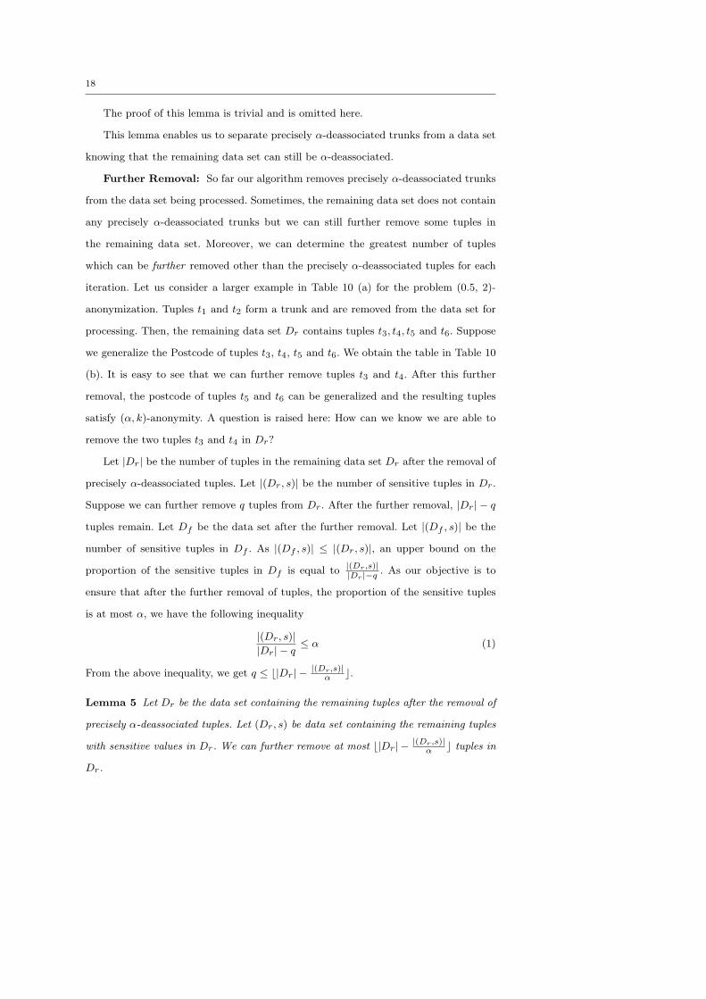
Further Removal: So far our algorithm removes precisely α-deassociated trunks

from the data set being processed. Sometimes, the remaining data set does not contain

any precisely α-deassociated trunks but we can still further remove some tuples in

the remaining data set. Moreover, we can determine the greatest number of tuples

which can be further removed other than the precisely α-deassociated tuples for each

iteration. Let us consider a larger example in Table 10 (a) for the problem (0.5, 2)-

anonymization. Tuples t1 and t2 form a trunk and are removed from the data set for

processing. Then, the remaining data set Dr contains tuples t3, t4, t5 and t6. Suppose

we generalize the Postcode of tuples t3, t4, t5 and t6. We obtain the table in Table 10

(b). It is easy to see that we can further remove tuples t3 and t4. After this further

removal, the postcode of tuples t5 and t6 can be generalized and the resulting tuples

satisfy (α, k)-anonymity. A question is raised here: How can we know we are able to

remove the two tuples t3 and t4 in Dr?

Let |Dr| be the number of tuples in the remaining data set Dr after the removal of

precisely α-deassociated tuples. Let |(Dr, s)| be the number of sensitive tuples in Dr.

Suppose we can further remove q tuples from Dr. After the further removal, |Dr| − q

tuples remain. Let Df be the data set after the further removal. Let |(Df , s)| be the

number of sensitive tuples in Df . As |(Df , s)| ≤ |(Dr, s)|, an upper bound on the

proportion of the sensitive tuples in Df is equal to|(Dr,s)||Dr|−q

. As our objective is to

ensure that after the further removal of tuples, the proportion of the sensitive tuples

is at most α, we have the following inequality

|(Dr, s)||Dr| − q

≤ α (1)

From the above inequality, we get q ≤ b|Dr| − |(Dr,s)|α c.

Lemma 5 Let Dr be the data set containing the remaining tuples after the removal of

precisely α-deassociated tuples. Let (Dr, s) be data set containing the remaining tuples

with sensitive values in Dr. We can further remove at most b|Dr| − |(Dr,s)|α c tuples in

Dr.

19

(a) (b)

Gender Birth Postcode Sens

male 1965 4351 n

male 1965 4351 c

male 1965 4351 n

male 1965 4352 n

male 1965 4363 n

male 1965 4374 c

Gender Birth Postcode Sens

male 1965 4351 n

male 1965 4351 c

male 1965 435* n

male 1965 435* n

male 1965 436* n

male 1965 437* c

Table 10 An Illustration of Further Removal

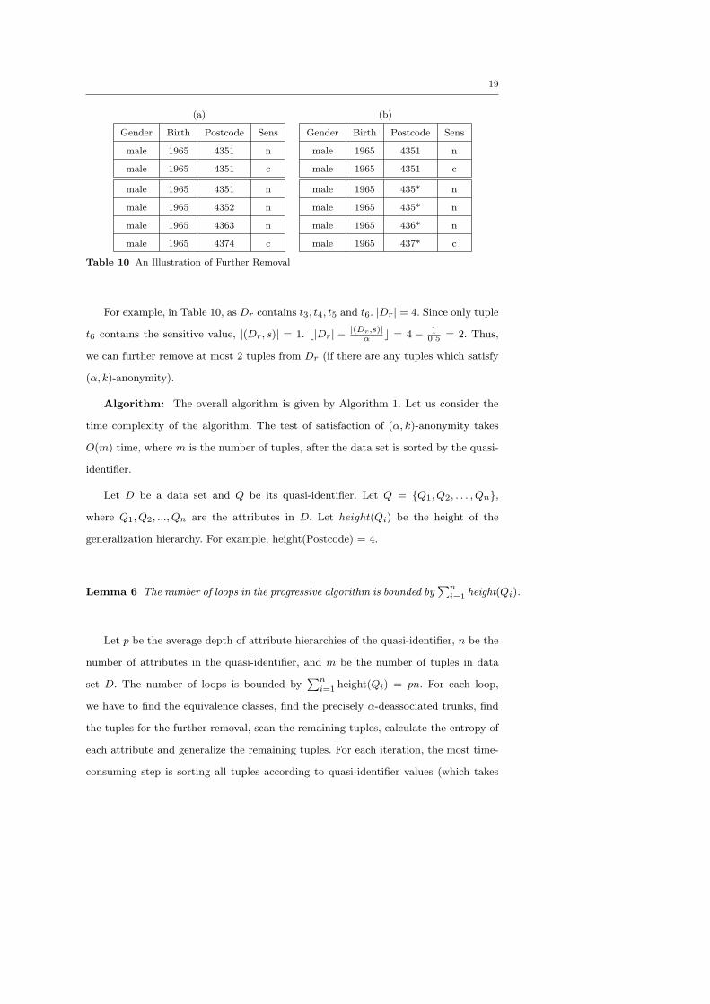
For example, in Table 10, as Dr contains t3, t4, t5 and t6. |Dr| = 4. Since only tuple

t6 contains the sensitive value, |(Dr, s)| = 1. b|Dr| − |(Dr,s)|α c = 4 − 1

0.5 = 2. Thus,

we can further remove at most 2 tuples from Dr (if there are any tuples which satisfy

(α, k)-anonymity).

Algorithm: The overall algorithm is given by Algorithm 1. Let us consider the

time complexity of the algorithm. The test of satisfaction of (α, k)-anonymity takes

O(m) time, where m is the number of tuples, after the data set is sorted by the quasi-

identifier.

Let D be a data set and Q be its quasi-identifier. Let Q = {Q1, Q2, . . . , Qn},where Q1, Q2, ..., Qn are the attributes in D. Let height(Qi) be the height of the

generalization hierarchy. For example, height(Postcode) = 4.

Lemma 6 The number of loops in the progressive algorithm is bounded by∑n

i=1 height(Qi).

Let p be the average depth of attribute hierarchies of the quasi-identifier, n be the

number of attributes in the quasi-identifier, and m be the number of tuples in data

set D. The number of loops is bounded by∑n

i=1 height(Qi) = pn. For each loop,

we have to find the equivalence classes, find the precisely α-deassociated trunks, find

the tuples for the further removal, scan the remaining tuples, calculate the entropy of

each attribute and generalize the remaining tuples. For each iteration, the most time-

consuming step is sorting all tuples according to quasi-identifier values (which takes

20

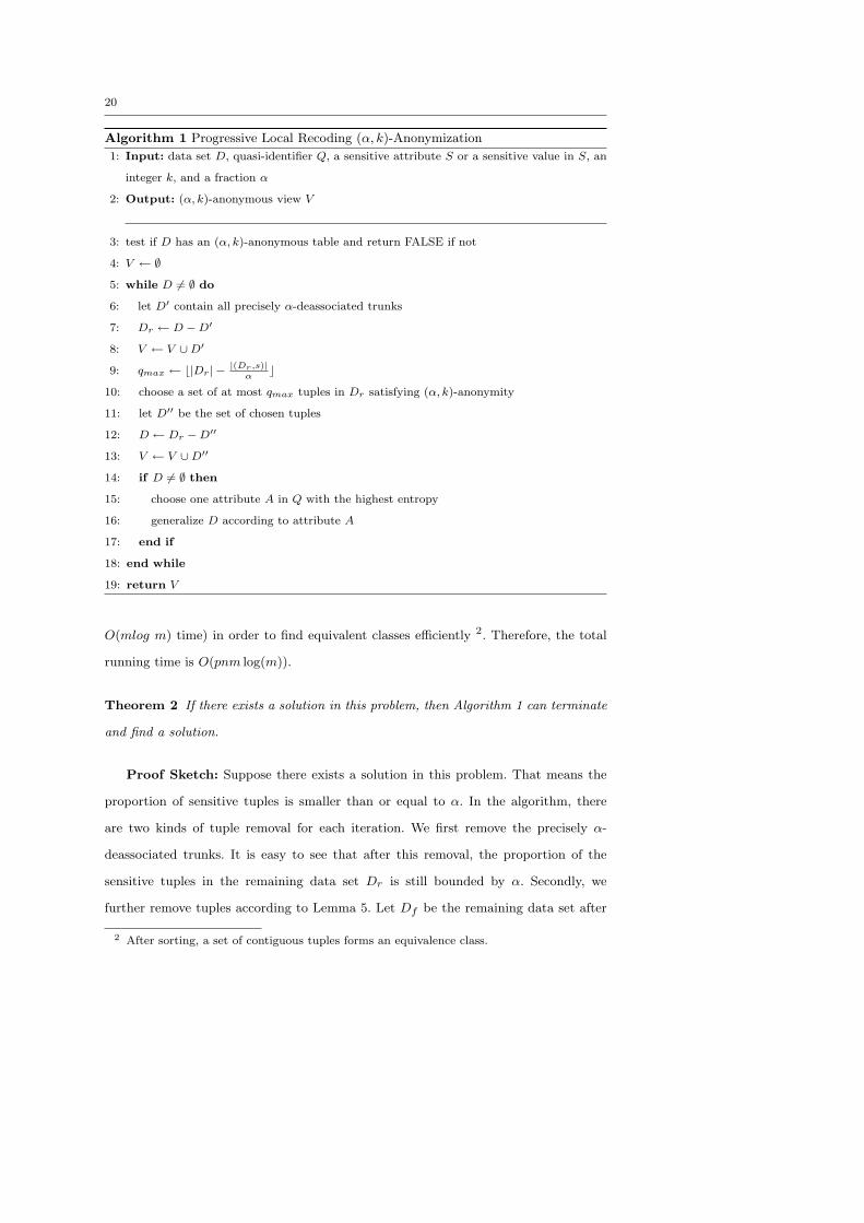
Algorithm 1 Progressive Local Recoding (α, k)-Anonymization

1: Input: data set D, quasi-identifier Q, a sensitive attribute S or a sensitive value in S, an

integer k, and a fraction α

2: Output: (α, k)-anonymous view V

3: test if D has an (α, k)-anonymous table and return FALSE if not

4: V ← ∅5: while D 6= ∅ do

6: let D′ contain all precisely α-deassociated trunks

7: Dr ← D −D′

8: V ← V ∪D′

9: qmax ← b|Dr| − |(Dr,s)|α

c10: choose a set of at most qmax tuples in Dr satisfying (α, k)-anonymity

11: let D′′ be the set of chosen tuples

12: D ← Dr −D′′

13: V ← V ∪D′′

14: if D 6= ∅ then

15: choose one attribute A in Q with the highest entropy

16: generalize D according to attribute A

17: end if

18: end while

19: return V

O(mlog m) time) in order to find equivalent classes efficiently 2. Therefore, the total

running time is O(pnm log(m)).

Theorem 2 If there exists a solution in this problem, then Algorithm 1 can terminate

and find a solution.

Proof Sketch: Suppose there exists a solution in this problem. That means the

proportion of sensitive tuples is smaller than or equal to α. In the algorithm, there

are two kinds of tuple removal for each iteration. We first remove the precisely α-

deassociated trunks. It is easy to see that after this removal, the proportion of the

sensitive tuples in the remaining data set Dr is still bounded by α. Secondly, we

further remove tuples according to Lemma 5. Let Df be the remaining data set after

2 After sorting, a set of contiguous tuples forms an equivalence class.

21

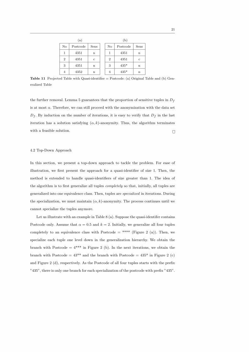
(a) (b)

No Postcode Sens

1 4351 n

2 4351 c

3 4351 n

4 4352 n

No Postcode Sens

1 4351 n

2 4351 c

3 435* n

4 435* n

Table 11 Projected Table with Quasi-identifier = Postcode: (a) Original Table and (b) Gen-

eralized Table

the further removal. Lemma 5 guarantees that the proportion of sensitive tuples in Df

is at most α. Therefore, we can still proceed with the anonymization with the data set

Df . By induction on the number of iterations, it is easy to verify that Df in the last

iteration has a solution satisfying (α, k)-anonymity. Thus, the algorithm terminates

with a feasible solution.

4.2 Top-Down Approach

In this section, we present a top-down approach to tackle the problem. For ease of

illustration, we first present the approach for a quasi-identifier of size 1. Then, the

method is extended to handle quasi-identifiers of size greater than 1. The idea of

the algorithm is to first generalize all tuples completely so that, initially, all tuples are

generalized into one equivalence class. Then, tuples are specialized in iterations. During

the specialization, we must maintain (α, k)-anonymity. The process continues until we

cannot specialize the tuples anymore.

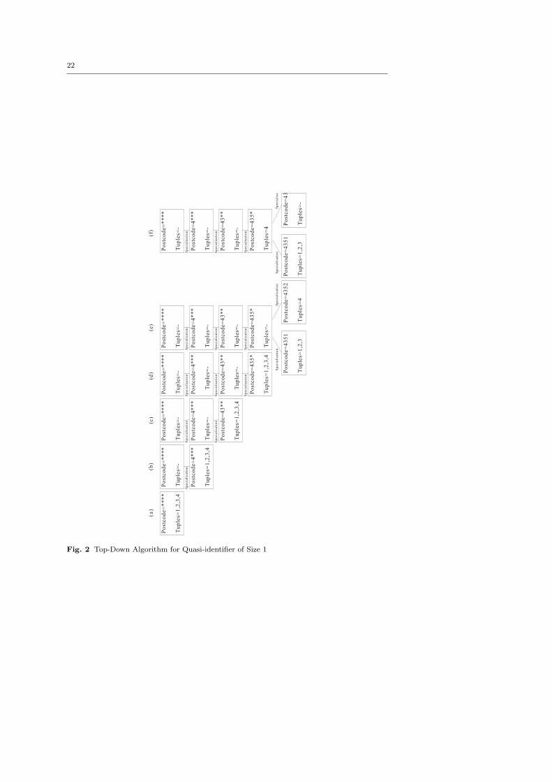
Let us illustrate with an example in Table 8 (a). Suppose the quasi-identifer contains

Postcode only. Assume that α = 0.5 and k = 2. Initially, we generalize all four tuples

completely to an equivalence class with Postcode = **** (Figure 2 (a)). Then, we

specialize each tuple one level down in the generalization hierarchy. We obtain the

branch with Postcode = 4*** in Figure 2 (b). In the next iterations, we obtain the

branch with Postcode = 43** and the branch with Postcode = 435* in Figure 2 (c)

and Figure 2 (d), respectively. As the Postcode of all four tuples starts with the prefix

”435”, there is only one branch for each specialization of the postcode with prefix ”435”.

22

Po

stco

de=

**

**

Tu

ple

s=1

,2,3

,4

Po

stco

de=

**

**

Tu

ple

s=-

Po

stco

de=

4*

**

Tu

ple

s=1

,2,3

,4

Sp

ecia

lisa

tio

n

Po

stco

de=

**

**

Tu

ple

s=-

Po

stco

de=

4*

**

Tu

ple

s=-

Sp

ecia

lisa

tio

n

Po

stco

de=

43

**

Tu

ple

s=1

,2,3

,4

Sp

ecia

lisa

tio

n

Po

stco

de=

**

**

Tu

ple

s=-

Po

stco

de=

4*

**

Tu

ple

s=-

Sp

ecia

lisa

tio

n

Po

stco

de=

43

**

Tu

ple

s=-

Sp

ecia

lisa

tio

n

Po

stco

de=

43

5*

Tu

ple

s=1

,2,3

,4

Sp

ecia

lisa

tio

n

Po

stco

de=

**

**

Tu

ple

s=-

Po

stco

de=

4*

**

Tu

ple

s=-

Sp

ecia

lisa

tio

n

Po

stco

de=

43

**

Tu

ple

s=-

Sp

ecia

lisa

tio

n

Po

stco

de=

43

5*

Tu

ple

s=-

Sp

ecia

lisa

tio

n

Po

stco

de=

43

51

Tu

ple

s=1

,2,3

Sp

ecia

lisa

tio

n

Po

stco

de=

43

52

Tu

ple

s=4

Sp

ecia

lisa

tio

n

Po

stco

de=

**

**

Tu

ple

s=-

Po

stco

de=

4*

**

Tu

ple

s=-

Sp

ecia

lisa

tio

n

Po

stco

de=

43

**

Tu

ple

s=-

Sp

ecia

lisa

tio

n

Po

stco

de=

43

5*

Tu

ple

s=4

Sp

ecia

lisa

tio

n

Po

stco

de=

43

51

Tu

ple

s=1

,2,3

Sp

ecia

lisa

tio

n

Po

stco

de=

43

52

Tu

ple

s=-

Sp

ecia

lisa

tio

n

Po

stco

de=

**

**

Tu

ple

s=-

Po

stco

de=

4*

**

Tu

ple

s=-

Sp

ecia

lisa

tio

n

Po

stco

de=

43

**

Tu

ple

s=-

Sp

ecia

lisa

tio

n

Po

stco

de=

43

5*

Tu

ple

s=3

,4

Sp

ecia

lisa

tio

n

Po

stco

de=

43

51

Tu

ple

s=1

,2

Sp

ecia

lisa

tio

n

Po

stco

de=

43

52

Tu

ple

s=-

Sp

ecia

lisa

tio

n

(a)

(b)

(c)

(d)

(e)

(f)

(g)

Fig. 2 Top-Down Algorithm for Quasi-identifier of Size 1

23

Next, we can further specialize the tuples into the two branches as shown Figure 2 (e).

Hence the specialization processing can be seen as the growth of a tree.

If each leaf node satisfies (α, k)-anonymity, then the specialization will be suc-

cessful. However, we may encounter some problematic leaf nodes that do not satisfy

(α, k)-anonymity. Then, all tuples in such leaf nodes will be pushed upwards in the

generalization hierarchy. In other words, those tuples cannot be specialized in this

process. They should be kept unspecialized in the parent node. For example, in Fig-

ure 2 (e), the leaf node with Postcode = 4352 contains only one tuple, which violates

(α, k)-anonymity, where k = 2. Thus, we have to move this tuple back to the parent

node with Postcode = 435*. See Figure 2 (f).

After the previous step, we move all tuples in problematic leaf nodes to the par-

ent node. However, if the collected tuples in the parent node do not satisfy (α, k)-

anonymity, we should further move some tuples from other leaf nodes L to the parent

node so that the parent node can satisfy (α, k)-anonymity while L also maintain the

(α, k)-anonymity. For instance, in Figure 2 (f), the parent node with Postcode = 435*

violates (α, k)-anonymity, where k = 2. Thus, we should move one tuples upwards in

the node B with Postcode = 4351 (which satisfies (α, k)-anonymity). In this example,

we move tuple 3 upwards to the parent node so that both the parent node and the

node B satisfy the (α, k)-anonymity.

Finally, in Figure 2 (g), we obtain a data set where the Postcode of tuples 3 and

4 are generalized to 435* and the Postcode of tuples 1 and 2 remains 4351. We call

the final allocation of tuples in Figure 2 (g) the final distribution of tuples after the

specialization. The results can be found in Table 11 (b).

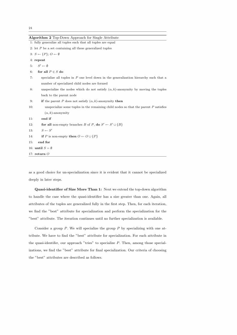
The pseudo-code of the algorithm is shown in Algorithm 2. In line 10 of Algorithm 2,

we have to un-specialize some tuples which have already satisfied the (α, k)-anonymity.

Which tuples should we select in order to produce a generalized data set with less dis-

tortion? We tackle this issue by the following additional steps. We further specializing

all tuples in all candidate nodes. We repeat the specialization process until we cannot

further specialize the tuples. Then, for each tuple t, we record the number of times of

specializations. If the tuple t has fewer times of specializations, it should be considered

24

Algorithm 2 Top-Down Approach for Single Attribute

1: fully generalize all tuples such that all tuples are equal

2: let P be a set containing all these generalized tuples

3: S ← {P}; O ← ∅4: repeat

5: S′ ← ∅6: for all P ∈ S do

7: specialize all tuples in P one level down in the generalization hierarchy such that a

number of specialized child nodes are formed

8: unspecialize the nodes which do not satisfy (α, k)-anonymity by moving the tuples

back to the parent node

9: if the parent P does not satisfy (α, k)-anonymity then

10: unspecialize some tuples in the remaining child nodes so that the parent P satisfies

(α, k)-anonymity

11: end if

12: for all non-empty branches B of P , do S′ ← S′ ∪ {B}13: S ← S′

14: if P is non-empty then O ← O ∪ {P}15: end for

16: until S = ∅17: return O

as a good choice for un-specialization since it is evident that it cannot be specialized

deeply in later steps.

Quasi-identifier of Size More Than 1: Next we extend the top-down algorithm

to handle the case where the quasi-identifier has a size greater than one. Again, all

attributes of the tuples are generalized fully in the first step. Then, for each iteration,

we find the ”best” attribute for specialization and perform the specialization for the

”best” attribute. The iteration continues until no further specialization is available.

Consider a group P . We will specialize the group P by specializing with one at-

tribute. We have to find the ”best” attribute for specialization. For each attribute in

the quasi-identifer, our approach ”tries” to specialize P . Then, among those special-

izations, we find the ”best” attribute for final specialization. Our criteria of choosing

the ”best” attributes are described as follows.

25

Postcode=****

Tuples=-

Postcode=4***

Tuples=1,2

Specialisation

Postcode=5***

Tuples=3,4

Specialisation

Birth=*

Tuples=3,4

Birth=1965

Tuples=1,2

Specialisation

Birth=1966

Tuples=-

Specialisation

(a) (b)

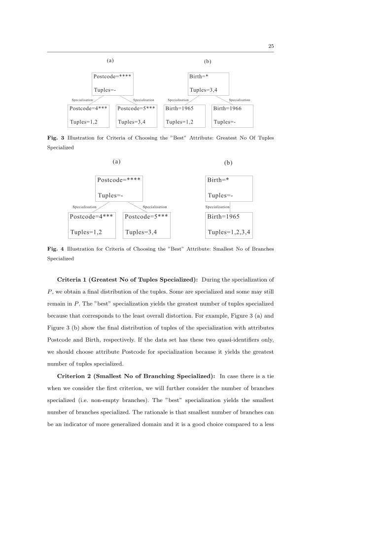
Fig. 3 Illustration for Criteria of Choosing the ”Best” Attribute: Greatest No Of Tuples

Specialized

Postcode=****

Tuples=-

Postcode=4***

Tuples=1,2

Specialisation

Postcode=5***

Tuples=3,4

Specialisation

Birth=*

Tuples=-

Birth=1965

Tuples=1,2,3,4

Specialisation

(a) (b)

Fig. 4 Illustration for Criteria of Choosing the ”Best” Attribute: Smallest No of Branches

Specialized

Criteria 1 (Greatest No of Tuples Specialized): During the specialization of

P , we obtain a final distribution of the tuples. Some are specialized and some may still

remain in P . The ”best” specialization yields the greatest number of tuples specialized

because that corresponds to the least overall distortion. For example, Figure 3 (a) and

Figure 3 (b) show the final distribution of tuples of the specialization with attributes

Postcode and Birth, respectively. If the data set has these two quasi-identifiers only,

we should choose attribute Postcode for specialization because it yields the greatest

number of tuples specialized.

Criterion 2 (Smallest No of Branching Specialized): In case there is a tie

when we consider the first criterion, we will further consider the number of branches

specialized (i.e. non-empty branches). The ”best” specialization yields the smallest

number of branches specialized. The rationale is that smallest number of branches can

be an indicator of more generalized domain and it is a good choice compared to a less

26

Attribute Distinct Values Generalizations Height

1 Age 74 5-, 10-, 20-year ranges 4

2 Work Class 7 Taxonomy Tree 3

3 Education 16 Taxonomy Tree 4

4 Martial Status 7 Taxonomy Tree 3

5 Occupation 14 Taxonomy Tree 2

6 Race 5 Taxonomy Tree 2

7 Sex 2 Suppression 1

8 Native Country 41 Taxonomy Tree 3

9 Salary Class 2 Suppression 1

Table 12 Description of Adult Data Set

generalized domain. For example, Figure 4 (a) and Figure 4 (b) shows the final distri-

bution of tuples of the specialization with attribute Postcode and Birth, respectively.

If the data set has these two quasi-identifiers only, we should choose attribute Birth

for specialization because it yields the smallest number of branches specialized.

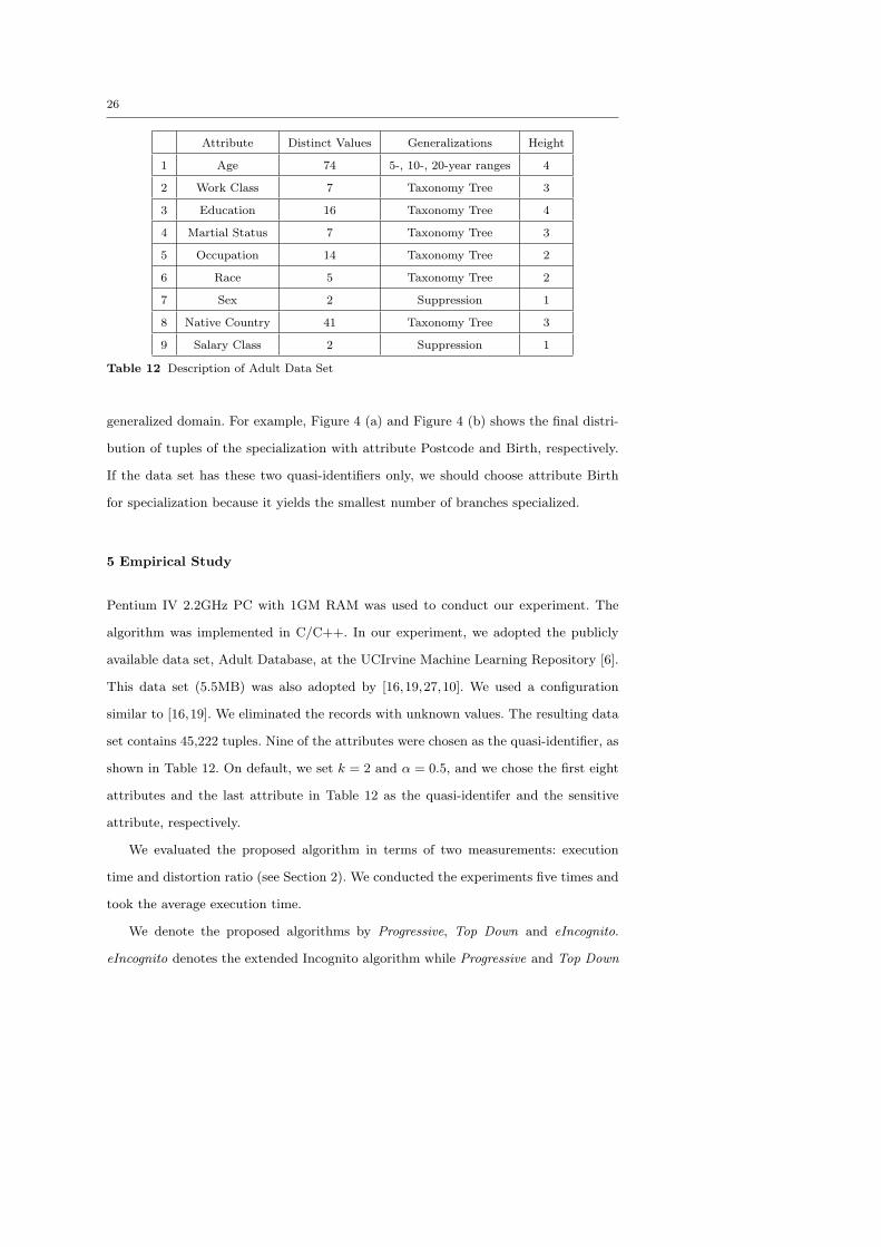
5 Empirical Study

Pentium IV 2.2GHz PC with 1GM RAM was used to conduct our experiment. The

algorithm was implemented in C/C++. In our experiment, we adopted the publicly

available data set, Adult Database, at the UCIrvine Machine Learning Repository [6].

This data set (5.5MB) was also adopted by [16,19,27,10]. We used a configuration

similar to [16,19]. We eliminated the records with unknown values. The resulting data

set contains 45,222 tuples. Nine of the attributes were chosen as the quasi-identifier, as

shown in Table 12. On default, we set k = 2 and α = 0.5, and we chose the first eight

attributes and the last attribute in Table 12 as the quasi-identifer and the sensitive

attribute, respectively.

We evaluated the proposed algorithm in terms of two measurements: execution

time and distortion ratio (see Section 2). We conducted the experiments five times and

took the average execution time.

We denote the proposed algorithms by Progressive, Top Down and eIncognito.

eIncognito denotes the extended Incognito algorithm while Progressive and Top Down

27

denote the local-recoding based progressive approach and the local-recoding based top-

down approach, respectively.

0

50

100

150

0 0.5 1

a

Exec

utionTime/s

0

50

100

150

0 5 10

Quasi-Identifier Size

ExecutionTime/s

Progressive

Top Down

eIncognito

(a) (b)

0

20

40

60

80

100

0 0.5 1

a

Distortion

Ratio/%

0

20

40

60

80

100

0 5 10

Quasi-Identifier Size

Distortion

Ratio/%

Progressive

Top Down

eIncognito

(c) (d)

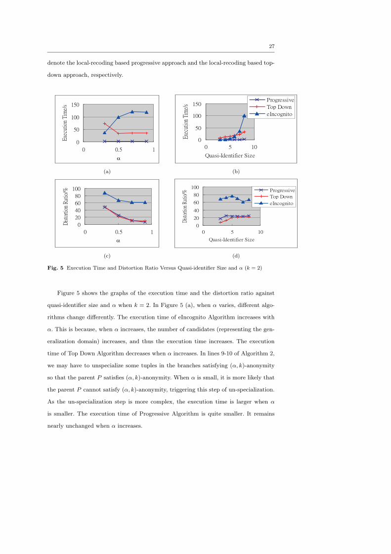
Fig. 5 Execution Time and Distortion Ratio Versus Quasi-identifier Size and α (k = 2)

Figure 5 shows the graphs of the execution time and the distortion ratio against

quasi-identifier size and α when k = 2. In Figure 5 (a), when α varies, different algo-

rithms change differently. The execution time of eIncognito Algorithm increases with

α. This is because, when α increases, the number of candidates (representing the gen-

eralization domain) increases, and thus the execution time increases. The execution

time of Top Down Algorithm decreases when α increases. In lines 9-10 of Algorithm 2,

we may have to unspecialize some tuples in the branches satisfying (α, k)-anonymity

so that the parent P satisfies (α, k)-anonymity. When α is small, it is more likely that

the parent P cannot satisfy (α, k)-anonymity, triggering this step of un-specialization.

As the un-specialization step is more complex, the execution time is larger when α

is smaller. The execution time of Progressive Algorithm is quite smaller. It remains

nearly unchanged when α increases.

28

0

20

40

60

80

100

0 0.5 1

a

Exec

utionTime/s

0

20

40

60

80

100

0 5 10

Quasi-Identifier Size

ExecutionTime/s

Progressive

Top Down

eIncognito

(a) (b)

0

20

40

60

80

100

0 0.5 1

a

Distortion

Ratio/%

0

20

40

60

80

100

0 5 10

Quasi-Identifier Size

Disto

rtion

Ratio

/%

Progressive

Top Down

eIncognito

(c) (d)

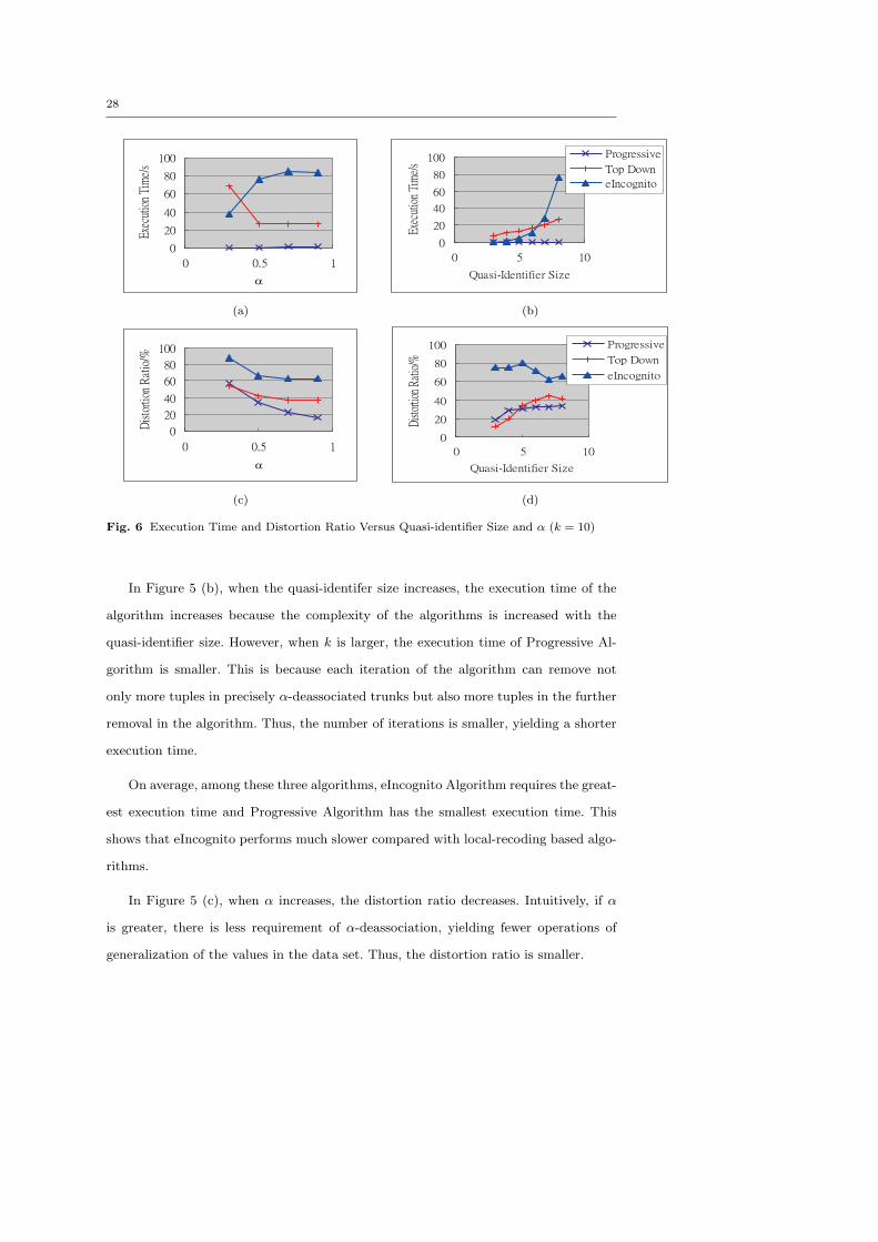
Fig. 6 Execution Time and Distortion Ratio Versus Quasi-identifier Size and α (k = 10)

In Figure 5 (b), when the quasi-identifer size increases, the execution time of the

algorithm increases because the complexity of the algorithms is increased with the

quasi-identifier size. However, when k is larger, the execution time of Progressive Al-

gorithm is smaller. This is because each iteration of the algorithm can remove not

only more tuples in precisely α-deassociated trunks but also more tuples in the further

removal in the algorithm. Thus, the number of iterations is smaller, yielding a shorter

execution time.

On average, among these three algorithms, eIncognito Algorithm requires the great-

est execution time and Progressive Algorithm has the smallest execution time. This

shows that eIncognito performs much slower compared with local-recoding based algo-

rithms.

In Figure 5 (c), when α increases, the distortion ratio decreases. Intuitively, if α

is greater, there is less requirement of α-deassociation, yielding fewer operations of

generalization of the values in the data set. Thus, the distortion ratio is smaller.

29

In Figure 5 (d), it is easy to see why the distortion ratio increases with the quasi-

identifier size. When the quasi-identifier contains more attributes, there is more chance

that the quasi-identifier of two tuples are different. In other words, there is more chance

that the tuples will be generalized. Thus, the distortion ratio is greater. When k is

larger, it is also obvious that the distortion ratio is greater because it is less likely that

the quasi-identifer of two tuples are equal.

On average, the local-recoding based algorithms (Progressive Algorithm and Top

Down Algorithm) result in about 3 times smaller distortion ratio compared with eIncog-

nito Algorithm. Also, the Progressive Algorithm and Top Down Algorithm generate

similar distortion ratio.

We have also conducted the experiments for k = 10, which is shown in Figure 6.

The results are also similar to the graphs for k = 2 (as in Figure 5). When k = 10 and

quasi-identifier size is large, the Top Down Algorithm gives a larger distortion ratio

than Progressive Algorithm. This can be explained by the fact that the Top Down

Algorithm considers the ”best” attributes independently among all attributes without

considering the relationship among attributes. Thus, when the quasi-identifier size (i.e.

the number of attributes) is larger, the performance is worse.

6 General (α, k)-anonymity model

In this section, we will extend the simple (α, k)-model to two different cases: (1) multiple

sensitive values in a single sensitive attribute (Section 6.1) and (2) multiple sensitive

values in multiple sensitive attributes (Section 6.2).

6.1 Multiple Sensitive Values

When there are two or more sensitive values and they are rare cases in a data set (e.g.

HIV and prostate cancer). We may combine them into one combined sensitive class

and the simple (α, k)-anonymity model is applicable. The inference confidence to each

individual sensitive value is smaller than or equal to the confidence to the combined

value, which is controlled by α.

30

Next we consider the case when all values in an attribute are sensitive and require

protection. It is possible to have an (α, k)-anonymity model to protect a sensitive

attribute when the attribute contains many values and no single value dominates the

attribute (which will be explained later). The salary attribute in employer table is an

example. When each equivalent class contains three salary scales with even distribution,

we have about 33% confidence to infer the salary scale of an individual in the equivalent

class.

Definition 10 (α-rare) Given an equivalence class E, an attribute X and an at-

tribute value x ∈ X. Let (E, x) be the set of tuples containing x in E and α be a

user-specified threshold, where 0 ≤ α ≤ 1. Equivalence class E is α-rare with respect

to attribute set X if the proportion of every attribute value of X in the data set is not

greater than α, i.e. |(E, x)|/|E| ≤ α for x ∈ X.

For example, in Table 3, if X = Illness, equivalent class {t3, t4} is 0.5-rare because

”flu” and ”fever” occur evenly in the equivalent class. If every equivalent class is α-rare

in the class, the data set is called α-deassociated.

Definition 11 (General α-deassociation property) Given a data set D, an at-

tribute set Q and a sensitive class attribute S. Let α be a user-specified threshold,

where 0 ≤ α ≤ 1. Data set D is said to satisfy general α-deassociation with respect to

an attribute set Q and a sensitive attribute S if, for any equivalent classes E ⊂ D, E

is α-rare with respect to S.

For example, Table 3 is 0.5-deassociated since all three equivalent classes, {t1, t6},{t2, t5} and {t3, t4}, are 0.5-rare with respect to attribute set Illness. When a data set

is α-deassociated with respect to a sensitive attribute, it is α-deassociated with respect

to every value in the attribute. Therefore, the upper bound of inference confidence

from the quasi-identifier to the sensitive attribute is α.

Definition 12 (General (α, k)-anonymity) Given an attribute set Q and a sensitive

class attribute S, a view of a table is said to be a general (α, k)-anonymization of the

table if the view modifies the table such that the view satisfies both k-anonymity and

general α-deassociation with respect to an attribute set Q and a sensitive attribute S.

31

The proposed algorithms in Sections 3 and 4 can be extended to the general (α, k)-

anonymity model. The global-recoding based algorithm depends on two major proper-

ties - the generalization property (Lemma 2) and the subset property (Lemma 3). Both

propoerties hold for the general (α, k)-anonymity. Thus, the global-recoding based al-

gorithm can be extended by modifying the step of testing of candidates with the general

model.

The progressive local-recoding algorithm contains three major components - (1)

Criteria of Choosing Attributes, (2) α-Deassociated Removal and (3) Further Removal.

(1) As the measurement for the criteria of choosing attribute is based on the quasi-

identifier but no sensitive attribute, this component can still be used directly. Although

we cannot apply (2), we can continue to use step (3), by modifying the bound of the

number of removal. Recall that we can further remove at most b|Dr|− |(Dr,s)|α c (Lemma

5) in the mode for a single sensitive value s. In the general mode, all sensitive values

should satisfy Equation (1). That is, the formula in Lemma 5 becomes b|Dr|− |(Dr,s)|α c

for all s ∈ S, where S is the sensitive attribute. As we make sure that all the sensitive

values in the sensitive attribute should satisfy the general (α, k)-anonymity, we should

remove at most mins∈S{b|Dr| − |(Dr,s)|α c}. After these modifications, the progressive

algorithm can handle the general model.

The top-down local-recoding algorithm can also be easily extended to the general

model by modifying the condition when testing the candidates.

6.2 Multiple Sensitive Attributes

In some cases, the table may contain multiple sensitive attributes. For example, in

addition to attribute Illness, there are some other sensitive attributes like Income in

the table. We can also easily extend our (α, k)-anonymity model in this case. Let S be

the set of sensitive attributes in the table. We can refine Definition 11 as follows.

Definition 13 (S-General α-deassociation property) Given a data set D, an

attribute set Q and a set S of sensitive attributes. Let α be a user-specified threshold,

where 0 ≤ α ≤ 1. Data set D is said to satisfy S-general α-deassociation with respect

32

to an attribute set Q and a set S if, for each S ∈ S, D satisfies general α-deassociation

with respect to Q and S.

Definition 14 (S-General (α, k)-anonymity) Given an attribute set Q and a set Sof sensitive attributes, a view of a table is said to be a S-general (α, k)-anonymization

of the table if the view modifies the table such that the view satisfies both k-anonymity

and S-general α-deassociation with respect to an attribute set Q and a set S.

Similarly, we can also adapt our algorithms as follows. Since the generalization

property and the subset property hold for the S-general (α, k)-anonymity, we can

modify the step of testing of candidates with this general model.

Similar to Section 6.1, in the progressive local-recoding algorithm, the first step

for “Criteria of Choosing Attributes” can still be used. For the third step, we should

remove at most mins∈S and S∈S{b|Dr| − |(Dr,s)|α c}.

Similarly, the top-down local-recoding algorithm can also be easily extended to the

general model by modifying the condition when testing the candidates.

7 Conclusion

The k-anonymity model protects identification information, but does not protect sen-

sitive relationships in a data set. In this paper, we propose the (α, k)-anonymity model

to protect both identifications and relationships in data. We discuss the properties of

the model. We prove that achieving optimal (α, k)-anonymity by local recoding is NP-

hard. We present an optimal global-recoding method and two efficient local-encoding

based algorithms to transform a data set to satisfy (α, k)-anonymity property. The

experiment shows that, on average, the two local-encoding based algorithms performs

about 4 times faster and gives about 3 times less distortions of the data set compared

with the global-recoding algorithm.

Acknowledgement

We are grateful to the anonymous reviewers for their constructive comments on this

paper. This research was supported in part by HKSAR RGC Direct Allocation Grant

33

DAG08/09.EG01 to Raymond Chi-Wing Wong, This research was supported by ARC

discovery grant DP0774450 to Jiuyong Li.

References

1. G. Aggarwal, T. Feder, K. Kenthapadi, R. Motwani, R. Panigrahy, D. Thomas, and A. Zhu.

Anonymizing tables. In ICDT, pages 246–258, 2005.

2. D. Agrawal and C. C. Aggarwal. On the design and quantification of privacy preserving

data mining algorithms. In PODS ’01: Proceedings of the twentieth ACM SIGMOD-

SIGACT-SIGART symposium on Principles of database systems, pages 247–255, New

York, NY, USA, 2001. ACM Press.

3. R. Agrawal and R. Srikant. Fast algorithms for mining association rules. In VLDB, 1994.

4. R. Agrawal and R. Srikant. Privacy-preserving data mining. In Proc. of the ACM SIGMOD

Conference on Management of Data, pages 439–450. ACM Press, May 2000.

5. R. Bayardo and R. Agrawal. Data privacy through optimal k-anonymization. In ICDE,

pages 217–228, 2005.

6. E. K. C. Blake and C. J. Merz. UCI repository of machine learning databases,

http://www.ics.uci.edu/∼mlearn/MLRepository.html, 1998.

7. Y. Bu, A. W.-C. Fu, R. C.-W. Wong, L. Chen, and J. Li. Privacy preserving serial data

publishing by role composition. In VLDB, 2008.

8. L. Cox. Suppression methodology and statistical disclosure control. J. American Statistical

Association, 75:377–385, 1980.

9. U. M. Fayyad and K. B. Irani. Multi-interval discretization of continuous-valued attributes

for classification learning. In Proceedings of the Thirteenth International Joint Confer-

ence on Artificial Intelligence (IJCAI-93), pages 1022–1027, San Francisco, 1993. Morgan

Kaufmann.

10. B. C. M. Fung, K. Wang, and P. S. Yu. Top-down specialization for information and

privacy preservation. In ICDE, pages 205–216, 2005.

11. I. Holyer. The np-completeness of some edge-partition problems. SIAM J. on Computing,

10(4):713–717, 1981.

12. A. Hundepool. The argus software in the casc-project: Casc project international work-

shop. In Privacy in Statistical Databases, volume 3050 of Lecture Notes in Computer

Science, pages 323–335, Barcelona, Spain, 2004. Springer.

13. A. Hundepool and L. Willenborg. µ-and τ - argus: software for statistical disclosure control.

In Third international seminar on statsitcal confidentiality, Bled, 1996.

14. V. S. Iyengar. Transforming data to satisfy privacy constraints. In KDD ’02: Proceedings

of the eighth ACM SIGKDD international conference on Knowledge discovery and data

mining, pages 279–288, 2002.

34

15. K. Wang, B. Fung and P. Yu, Handicapping attacker’s confidence: An alternative to k-

anonymization. In Knowledge and Information Systems: An International Journal, 11(3),

2007.

16. K. LeFevre, D. J. DeWitt, and R. Ramakrishnan. Incognito: Efficient full-domain k-

anonymity. In SIGMOD Conference, pages 49–60, 2005.

17. J. Li, R. C.-W. Wong, A. W.-C. Fu, and J. Pei. Achieving k-anonymity by clustering in

attribute hierarchical structures. In DaWaK, 2006.

18. N. Li and T. Li. t-closeness: Privacy beyond k-anonymity and l-diversity. In ICDE, 2007.

19. A. Machanavajjhala, J. Gehrke, and D. Kifer. l-diversity: privacy beyond k-anonymity. In

To appear in ICDE06, 2006.

20. A. Meyerson and R. Williams. On the complexity of optimal k-anonymity. In PODS,

pages 223–228, 2004.

21. S. Rizvi and J. Haritsa. Maintaining data privacy in association rule mining. In Proceed-

ings of the 28th Conference on Very Large Data Base (VLDB02), pages 682–693. VLDB

Endowment, 2002.

22. P. Samarati. Protecting respondents’ identities in microdata release. IEEE Transactions

on Knowledge and Data Engineering, 13(6):1010–1027, 2001.

23. L. Sweeney. Achieving k-anonymity privacy protection using generalization and sup-

pression. International journal on uncertainty, Fuzziness and knowldege based systems,

10(5):571 – 588, 2002.

24. L. Sweeney. k-anonymity: a model for protecting privacy. International journal on uncer-

tainty, Fuzziness and knowldege based systems, 10(5):557 – 570, 2002.

25. V. S. Verykios, A. K. Elmagarmid, E. Bertino, Y. Saygin, and E. Dasseni. Association rule

hiding. IEEE Transactions on Knowledge and Data Engineering, 16(4):434–447, 2004.

26. K. Wang, B. C. M. Fung, and P. S. Yu. Template-based privacy preservation in classifica-

tion problems. In To appear in ICDM05, 2005.

27. K. Wang, P. S. Yu, and S. Chakraborty. Bottom-up generalization: A data mining solution

to privacy protection. In ICDM, pages 249–256, 2004.

28. L. Willenborg and T. de Waal. Statistical disclosure control in practice. Lecture Notes in

Statistics, 111, 1996.

29. X. Xiao and Y. Tao. Personalized privacy preservation. In SIGMOD, 2006.

30. X. Xiao and Y. Tao. m-invariance: Towards privacy preserving re-publication of dynamic

datasets. In SIGMOD, 2007.

31. J. Xu, W. Wang, J. Pei, X. Wang, B. Shi, and A. Fu. Utility-based anonymization using

local recoding. In KDD, 2006.