J Intell Inf Syst (2009) 33:209–234DOI 10.1007/s10844-008-0075-2

(α, k)-anonymous data publishing

Raymond Wong · Jiuyong Li ·Ada Fu · Ke Wang

Received: 2 June 2008 / Revised: 25 November 2008 /Accepted: 25 November 2008 / Published online: 8 January 2009© Springer Science + Business Media, LLC 2008

Abstract Privacy preservation is an important issue in the release of data for miningpurposes. The k-anonymity model has been introduced for protecting individualidentification. Recent studies show that a more sophisticated model is necessaryto protect the association of individuals to sensitive information. In this paper, wepropose an (α, k)-anonymity model to protect both identifications and relationshipsto sensitive information in data. We discuss the properties of (α, k)-anonymity model.We prove that the optimal (α, k)-anonymity problem is NP-hard. We first present anoptimal global-recoding method for the (α, k)-anonymity problem. Next we proposetwo scalable local-recoding algorithms which are both more scalable and result in lessdata distortion. The effectiveness and efficiency are shown by experiments. We alsodescribe how the model can be extended to more general cases.

Keywords Privacy · Data mining · Anonymity ·Privacy preservation · Data publishing

R. WongDepartment of Computer Science and Engineering,Hong Kong University of Science and Technology,Kowloon, Hong Kong

J. Li (B)School of Computer and Information Sciences, University of South Australia,Mawson Lakes, South Australia, Australiae-mail: jiuyong.li@unisa.edu.au

A. FuDepartment of Computer Science and Engineering,Chinese University of Hong Kong,Shatin, Hong Kong

K. WangDepartment of Computer Science, Simon Fraser University,Burnaby, Canada

210 J Intell Inf Syst (2009) 33:209–234

1 Introduction

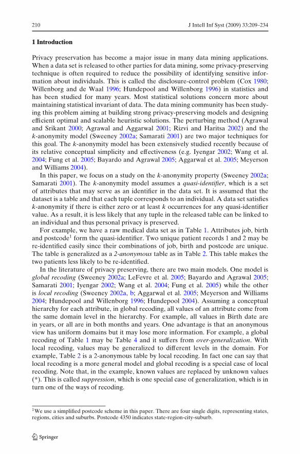
Privacy preservation has become a major issue in many data mining applications.When a data set is released to other parties for data mining, some privacy-preservingtechnique is often required to reduce the possibility of identifying sensitive infor-mation about individuals. This is called the disclosure-control problem (Cox 1980;Willenborg and de Waal 1996; Hundepool and Willenborg 1996) in statistics andhas been studied for many years. Most statistical solutions concern more aboutmaintaining statistical invariant of data. The data mining community has been study-ing this problem aiming at building strong privacy-preserving models and designingefficient optimal and scalable heuristic solutions. The perturbing method (Agrawaland Srikant 2000; Agrawal and Aggarwal 2001; Rizvi and Haritsa 2002) and thek-anonymity model (Sweeney 2002a; Samarati 2001) are two major techniques forthis goal. The k-anonymity model has been extensively studied recently because ofits relative conceptual simplicity and effectiveness (e.g. Iyengar 2002; Wang et al.2004; Fung et al. 2005; Bayardo and Agrawal 2005; Aggarwal et al. 2005; Meyersonand Williams 2004).

In this paper, we focus on a study on the k-anonymity property (Sweeney 2002a;Samarati 2001). The k-anonymity model assumes a quasi-identifier, which is a setof attributes that may serve as an identifier in the data set. It is assumed that thedataset is a table and that each tuple corresponds to an individual. A data set satisfiesk-anonymity if there is either zero or at least k occurrences for any quasi-identifiervalue. As a result, it is less likely that any tuple in the released table can be linked toan individual and thus personal privacy is preserved.

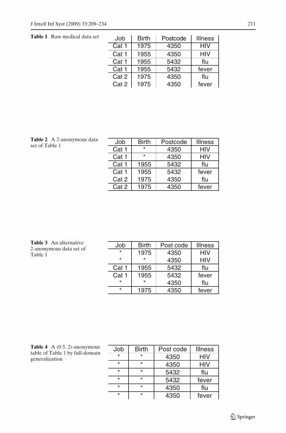
For example, we have a raw medical data set as in Table 1. Attributes job, birthand postcode1 form the quasi-identifier. Two unique patient records 1 and 2 may bere-identified easily since their combinations of job, birth and postcode are unique.The table is generalized as a 2-anonymous table as in Table 2. This table makes thetwo patients less likely to be re-identified.

In the literature of privacy preserving, there are two main models. One model isglobal recoding (Sweeney 2002a; LeFevre et al. 2005; Bayardo and Agrawal 2005;Samarati 2001; Iyengar 2002; Wang et al. 2004; Fung et al. 2005) while the otheris local recoding (Sweeney 2002a, b; Aggarwal et al. 2005; Meyerson and Williams2004; Hundepool and Willenborg 1996; Hundepool 2004). Assuming a conceptualhierarchy for each attribute, in global recoding, all values of an attribute come fromthe same domain level in the hierarchy. For example, all values in Birth date arein years, or all are in both months and years. One advantage is that an anonymousview has uniform domains but it may lose more information. For example, a globalrecoding of Table 1 may be Table 4 and it suffers from over-generalization. Withlocal recoding, values may be generalized to different levels in the domain. Forexample, Table 2 is a 2-anonymous table by local recoding. In fact one can say thatlocal recoding is a more general model and global recoding is a special case of localrecoding. Note that, in the example, known values are replaced by unknown values(*). This is called suppression, which is one special case of generalization, which is inturn one of the ways of recoding.

1We use a simplified postcode scheme in this paper. There are four single digits, representing states,regions, cities and suburbs. Postcode 4350 indicates state-region-city-suburb.

J Intell Inf Syst (2009) 33:209–234 211

Table 1 Raw medical data set Job Birth Postcode IllnessCat 1 1975 4350 HIVCat 1 1955 4350 HIVCat 1 1955 5432 fluCat 1 1955 5432 feverCat 2 1975 4350 fluCat 2 1975 4350 fever

Table 2 A 2-anonymous dataset of Table 1

Job Birth Postcode IllnessCat 1 * 4350 HIVCat 1 * 4350 HIVCat 1 1955 5432 fluCat 1 1955 5432 feverCat 2 1975 4350 fluCat 2 1975 4350 fever

Table 3 An alternative2-anonymous data set ofTable 1

Job Birth Post code Illness* 1975 4350 HIV* * 4350 HIV

Cat 1 1955 5432 fluCat 1 1955 5432 fever

* * 4350 flu* 1975 4350 fever

Table 4 A (0.5, 2)-anonymoustable of Table 1 by full-domaingeneralization

Job Birth Post code Illness* * 4350 HIV* * 4350 HIV* * 5432 flu* * 5432 fever* * 4350 flu* * 4350 fever

212 J Intell Inf Syst (2009) 33:209–234

Let us return to the earlier example. If we inspect Table 2 again, we can see thatthough it satisfies 2-anonymity property, it does not protect two patients’ sensitiveinformation, HIV infection. We may not be able to distinguish the two individualsfor the first two tuples, but we can derive the fact that both of them are HIVinfectious. Suppose one of them is the mayor, we can then confirm that the mayor hascontracted HIV. Surely, this is an undesirable outcome. Note that this is a problembecause the other individual whose generalized identifying attributes are the sameas the mayor also has HIV. Table 3 is an appropriate solution. Since (*,1975,4350)is linked to multiple diseases (i.e. HIV and fever) and (*,*,4350) is also linked tomultiple diseases (i.e. HIV and flu), it protects individual identifications and hidesthe implication.

We see from the above that protection of relationship to sensitive attribute valuesis as important as identification protection. Thus there are two goals for privacypreservation: (1) to protect individual identifications and (2) to protect sensitiverelationships. Our focus in this paper is to build a model to protect both in a discloseddata set. We propose an (α, k)-anonymity model, where α is a fraction and k is aninteger. In addition to k-anonymity, we require that, after anonymization, in anyequivalence class, the frequency (in fraction) of a sensitive value is no more than α.We first extend the well-known k-anonymity algorithm Incognito (LeFevre et al.2005) to our (α, k)-anonymity problem. As the algorithm is not scalable to the size ofquasi-identifier and may give a lot of distortions to the data since it is global-recodingbased, we also propose two efficient local-recoding based methods.

This proposal is different from the work of association rules hiding (Verykios et al.2004) in a transactional data set, where the rules to be hidden have to be knownbeforehand and each time only one rule can be hidden. Also, the implementationassumes that frequent itemsets of rules are disjoint, which is unrealistic. Our schemeblocks all rules from quasi-identifications to a sensitive class.

This work is also different from the work of template-based privacy preservationin classification problems (Wang et al. 2005, 2007), which considers hiding strong as-sociations between some attributes and sensitive classes and combines k-anonymitywith association hiding. There, the solution considers global recoding by suppressiononly and the aim is to minimize a distortion effect that is designed and dedicatedfor a classification problem. The model defined in this paper is more general inthat we allow local recoding and that we aim at minimizing the distortions of datamodifications without any attachment to a particular data mining method such asclassification.

This work is proposed to handle the homogeneity attack as l-diversitymodel (Machanavajjhala et al. 2006) does. Homogeneity attack is possible when agroup of individuals, whose identities are indistinguishable in a published table, sharethe same sensitive value. In other words, an attacker does not need to identify anindividual from a group, but can learn his/her sensitive information. We handle theproblem in a different way from l-diversity model. l-diversity model requires thatthe sensitive values of every identity undistinguishable group in a published tablehas at least l different sensitive values. This gives a general principle for handlingthe homogeneity attack, but l-diversity model suffers a major problem in practice.l-diversity does not specify the protective strength in terms of probability of leakage.Note that l-diversity does not mean that the probability of knowing one’s sensitivevalue is less than 1/ l when the distribution of sensitive values is skewed. Also,

J Intell Inf Syst (2009) 33:209–234 213

it is quite difficult for users to set parameter l. In contrast, α in our model is aprobabilistic parameter and is intuitive to set. Furthermore, the proposed algorithmin Machanavajjhala et al. (2006) is based on a global-recoding algorithm Incognito,which may generate more distortion compared to a local recoding approach. Wepropose two local recoding algorithms which can give low information loss.

It is worth mentioning other works (Li and Li 2007; Xiao and Tao 2006, 2007;Bu et al. 2008) which are also related to us although they are different from us.Li and Li (2007) proposed a privacy model called t-closeness. With this model,the distribution in each A-group in T∗ with respect to the sensitive attribute isroughly equal to the distribution of the entire table T∗. The difference betweenthe distribution in each A-group and the distribution of the entire table should bebounded with a parameter t. However, similar to l-diversity, it is difficult for the usersto set parameter t since parameter t is not intuitive. Xiao and Tao (2006) proposed apersonalized privacy model such that each individual can provide his/her preferenceon the protection of his/her sensitive value. The above works study the problemfor a one-time publication. Xiao and Tao (2007) and Bu et al. (2008) proposed theproblems for multiple-time publications. In this paper, we focus on the one-timepublication.

We propose to handle issues of k-anonymity with protection of some sensitivevalues. This is based on the fact that we could not protect too many sensitive valuesin a data set. If we do, a published data set may be hardly useful because of too manydistortions have been done to the data set. Practically, not all sensitive informationis considered as privacy. For example, people care more about depression thanvirus infection. We consider our proposed method as a practical enhancement ofk-anonymity with the consideration of the utility of published data.

Our Contributions:

– We propose a simple and effective model to protect both identifications andsensitive associations in a disclosed data set. The model extends the k-anonymitymodel to the (α, k)-anonymity model to limit the confidence of the implicationsfrom the quasi-identifier to a sensitive value (attribute) to within α in order toprotect the sensitive information from being inferred by strong implications. Weprove that the optimal (α, k)-anonymity by local recoding is NP-hard.

– We extend Incognito (LeFevre et al. 2005), a global-recoding algorithm for the k-anonymity problem, to solve this problem for (α, k)-anonymity. We also proposetwo local-recoding algorithms, which are scalable and generate less distortion.In our experiment, we show that, on average, the two local-recoding basedalgorithms performs about 4 times faster and gives about 3 times less distortionsof the data set compared with the extended Incognito algorithm.

2 Problem definition

We assume that each attribute has a corresponding conceptual hierarchy or taxon-omy. A lower level domain in the hierarchy provides more details than a higher leveldomain. For example, birth date in D/M/Y (e.g. 15/Mar/1970) is a lower level domainand birth date in Y (e.g. 1970) is a higher level domain. We assume such hierarchiesfor numerical attributes too. In particular, we have a hierarchical structure defined

214 J Intell Inf Syst (2009) 33:209–234

with {value, interval, *}, where value is the raw numerical data, interval is the range ofthe raw data and * is a symbol representing any values. Intervals can be determinedby users or a machine learning algorithm (Fayyad and Irani 1993). In a hierarchydomains with fewer values are more general than domains with more values for anattribute. The most general domain contains only one value. For example, 10-yearinterval level in birth domain is more general than one-year level. The most generallevel of birth domain contains value unknown (e.g. *). Generalization replaces lowerlevel domain values with higher level domain values. For example, birth D/M/Y isreplaced by M/Y.

Let D be a data set or a table. A record of D is a tuple or a row. An attributedefines all the possible values in a column. For a data set to be disclosed, any identifiercolumn (e.g. secure id and passport number) is definitely removed. However, someattribute combinations after this removal may still identify some individuals.

Definition 1 (Quasi-identifier) A quasi-identifier is a minimum set of attributes of Dthat may serve as identifications for some tuples in D.

For example, domain expert may decide that the attribute set {Job, Birth, Post-code} in Tables 1–4 is a quasi-identifier. The first goal of privacy preserving isto remove all possible identifications in a disclosed table (according to the quasi-identifer) so that individuals are not identifiable. We define an important concept,equivalence class, which is fundamental to our (α, k)-anonymity model.

Definition 2 (Equivalence Class) Let Q be an attribute set. An equivalence class of atable with respect to attribute set Q is a collection of all tuples in the table containingidentical values for attribute set Q.

For example, tuples 1 and 2 in Table 2 form an equivalence class with respectto attribute set {Job, Birth, Postcode}. The size of an equivalence class indicatesthe strength of identification protection of individuals in the equivalent class. If thenumber of tuples in an equivalence class is greater, it will be more difficult to re-identify individual.

Definition 3 (k-Anonymity Property) Let Q be an attribute set. A data set D isk-anonymous with respect to attribute set Q if the size of every equivalence classwith respect to attribute set Q is k or more.

The k-anonymity model requires that every value set for the quasi-identifierattribute set has a frequency of zero or at least k. For example, Table 1 does notsatisfy 2-anonymity property since tuples {Cat1, 1975, 4350} and {Cat1, 1955, 4350}occur once. Table 2 satisfies 2-anonymity property. Consider a large collection ofpatient records with different medical conditions. Some diseases are sensitive, suchas HIV, but many diseases are common, such as cold and fever. Only associationswith sensitive diseases need protection. To start with, we assume only one sensitivevalue, such as HIV. We introduce the α-deassociation requirement for the protection.

Definition 4 (α-Deassociation Requirement) Given a data set D, an attribute set Qand a sensitive value s in the domain of attribute S �∈ Q. Let (E, s) be the set oftuples in equivalence class E containing s for S. and α be a user-specified threshold,

J Intell Inf Syst (2009) 33:209–234 215

where 0 < α < 1. Data set D is α-deassociated with respect to attribute set Q and thesensitive value s if the frequency (in fraction) of s in every equivalence class is lessthan or equal to α. That is, |(E, s)|/|E| ≤ α for all equivalence classes E.

For example, Table 3 is 0.5-deassociated with respect to attribute set {Job, Birth,Postcode} and sensitive value HIV. There are three equivalence classes: {t1, t6}, {t2, t5}and {t3, t4}. For each of the first two equivalent classes of size two, only one tuplecontains HIV and therefore |(E, s)|/|E| = 0.5. For the third equivalence class, notuple contains HIV and therefore |(E, s)|/|E| = 0. Thus, for any equivalence classes,|(E, s)|/|E| ≤ 0.5.

However, the above definition may be too restrictive. For example, suppose k isset to 2 and α is set to 0.1. If the equivalence class contains two tuples, there shouldnot be any tuples containing the sensitive value because the greatest possible numberof tuples containing the sensitive value |(E, s)| is equal to α × |E| = 0.1 × 2 = 0.2,which is smaller than one. If all equivalence classes contain only two tuples, thenno equivalence classes can store any tuple containing the sensitive value, which isan undesirable result. One solution to this is to generate equivalence classes E ofgreater size such that α × |E| should be at least equal to 1. But, this solution maylead to unnecessary generalizaton. Therefore our solution is to introduce a ceiling tothe formula α × |E|.

Definition 5 (Refined α-Deassociation) Given a data set D, an attribute set Q anda sensitive value s in the domain of attribute S �∈ Q. Let (E, s) be the set of tuplesin equivalence class E containing s and α be a user-specified threshold, where 0 < α

< 1. Data set D is α-deassociated with respect to attribute set Q and the sensitivevalue s if the number of tuples containing s in every equivalence class is less than orequal to �α|E|�, i.e. |(E, s)| ≤ �α|E|� for all equivalence classes E.

Our objective is therefore to anonymize a data set so that it satisfies both thek-anonymity and the α-deassociation criteria.

Definition 6 ((α, k)-Anonymization) A view of a table is said to be an (α, k)-anonymization of the table if the view modifies the table such that the view satisfiesboth k-anonymity and α-deassociation properties with respect to the quasi-identifier.

For example, Table 3 is a (0.5, 2)-anonymous view of Table 1 since the size of allequivalence classes with respect to the quasi-identifier is 2 and each equivalence classcontains at most half of the tuples associating with HIV.

Both parameters α and k are intuitive and operable in real-world applications.Parameter α caps the confidence of implications from values in the quasi-identifierto the sensitive value while parameter k specifies the minimum number of identicalquasi-identifications.

Definition 7 (Local Recoding) Given a data set D of tuples, a function c that converteach tuple t in D to c(t) is a local recoding for D.

Local recoding typically distorts the values in the tuples in a data set. We candefine a measurement for the amount of distortion generated by a recoding, which

216 J Intell Inf Syst (2009) 33:209–234

we shall call the recoding cost. If a suppression is used for recoding of a value whichmodifies the value to an unknown *, then the cost can be measured by the totalnumber of suppressions, or the number of *’s in the resulting data set. Our objectiveis to find local recoding with a minimum cost. We call it the problem of optimal(α, k)-anonymization. The corresponding decision problem is defined as follows.

(α, k)-ANONYMIZATION: Given a data set D with a quasi-identifier Q anda sensitive value s, is there a local recoding for D by a function c such that, afterrecoding, (α, k)-anonymity is satisfied and the cost of the recoding is at most C?

Optimal k-anonymization by local recoding is NP-hard as discussed in Meyersonand Williams (2004) and Aggarwal et al. (2005). Now, we show that optimal (α, k)-anonymization by local recoding is also NP-hard.

Theorem 1 (α, k)-anonymity is NP-hard for a binary alphabet (∑ = {0, 1} ).

Proof Sketch The proof is by transforming the problem of EDGE PARTITIONINTO 4-CLIQUES to the (α, k)-anonymity problem.

Edge partition into 4-cliques: Given a simple graph G = (V, E), with |E| = 6m forsome integer m, can the edges of G be partitioned into m edge-disjoint 4-cliques?(Holyer 1981)

Given an instance of EDGE PARTITION INTO 4-CLIQUES. Set α = 0.5 andk = 12. For each vertex v ∈ V, construct a non-sensitive attribute. For each edgee ∈ E, where e = (v1, v2), create a pair of records rv1,v2 and r̃v1,v2 , where the tworecords have the attribute values of both v1 and v2 equal to 1 and all other non-sensitive attribute values equal to 0, but one record rv1,v2 has the sensitive attributeequal to 1 and the other record r̃v1,v2 has the sensitive attribute equal to 0.

We define the cost of the (0.5, 12)-anonymity to be the number of suppressionsapplied in the data set. We show that the cost of the (0.5, 12)-anonymity is at most48m if and only if E can be partitioned into a collection of m edge-disjoint 4-cliques.

Suppose E can be partitioned into a collection of m disjoint 4-cliques. Consider a4-clique Q with vertices v1, v2, v3and v4. If we suppress the attributes v1, v2, v3 and v4

in the 12 records corresponding to the edges in Q, then a cluster of these 12 recordsare formed where each modified record has four *’s. Note that the α-deassociationrequirement can be satisfied as the frequency of the sensitive attribute value 1 isequal to 0.5. The cost of the (0.5, 12)-anonymity is equal to 12 × 4 × m = 48m.

Suppose the cost of the (0.5, 12)-anonymity is at most 48m. As G is a simple graph,any twelve records should have at least four attributes different. So, each recordshould have at least four *’s in the solution of the (0.5, 12)-anonymity. Then, thecost of the (0.5, 12)-anonymity is at least 12 × 4 × m = 48m. Combining with theproposition that the cost is at most 48m, we obtain the cost is exactly equal to 48mand thus each record should have exactly four *’s in the solution. Each cluster shouldhave exactly 12 records (where six have sensitive value 1 and the other six havesensitive value 0). Suppose the twelve modified records contain four *’s in attributesv1, v2, v3 and v4, the records contain 0’s in all other non-sensitive attributes. Thiscorresponds to a 4-clique with vertices v1, v2, v3 and v4. Thus, we conclude that thesolution corresponds to a partition into a collection of m edge-disjoint 4-cliques. �

Let p be the fraction of the set of tuples that contain sensitive values. Suppose α isset smaller than p. Then no matter how we partition the data set, by the pigeon hole

J Intell Inf Syst (2009) 33:209–234 217

principle, there should be at least one partition P which contains p or more sensitivevalue, and therefore cannot satisfy α-deassociation property.

Lemma 1 (Choice of α) α should be set to a value greater than or equal to thefrequency (given in fraction) of the sensitive value in the data set D.

Distortion Ratio or Recoding Cost: Since we want to analyze the published data, itis interesting to see how large the distortion is the published data. There are manyutility metrics (Machanavajjhala et al. 2006; Xu et al. 2006; Li et al. 2006) to define thedistortion ratio of a published table. For example, in Machanavajjhala et al. (2006), ametric can be the average size of the equivalence classes without using the taxonomytrees for attributes. Xu et al. (2006) and Li et al. (2006) define more complicatedmetrics with the use of the taxonomy trees.

In this paper, we focus on the following distortion ratio. Note that how to definedistortion ratio is orthogonal to our (α, k)-anonymity model. Since we assume themore general case of a taxonomy tree for each attribute, we define the cost of local-recoding based on this model. The cost is given by the distortion ratio of the resultingdata set and is defined as follows. Suppose the value of the attribute of a tuplehas not been generalized, there will be no distortion. However, if the value of theattribute of a tuple is generalized to a more general value in the taxonomy tree,there is a distortion of the attribute of the tuple. If the value is generalized more (i.e.the original value is updated to a value at the node of the taxonomy near to theroot), the distortion will be greater. Thus, the distortion of this value is defined interms of the height of the value generalized. For example, if the value has not beengeneralized, the height of the value generalized is equal to 0. If the value has beengeneralized one level up in the taxonomy, the height of the value generalized is equalto 1. Let hi, j be the height of the value generalized of attribute Ai of the tuple t j. Thedistortion of the whole data set is equal to the sum of the distortions of all values inthe generalized data set. That is, distortion =

∑i, j hi, j. Distortion ratio is equal to the

distortion of the generalized data set divided by the distortion of the fully generalizeddata set, where the fully generalized data set is one with all values of the attributesare generalized to the root of the taxonomy.

3 Global-recoding

In this section, we extend an existing global-recoding based algorithm called Incog-nito (LeFevre et al. 2005) for the (α, k)-anonymous model. Incognito algorithm(LeFevre et al. 2005) is an optimal algorithm for the k-anonymity problem. It hasalso been used in Machanavajjhala et al. (2006) for the l-diversity problem.

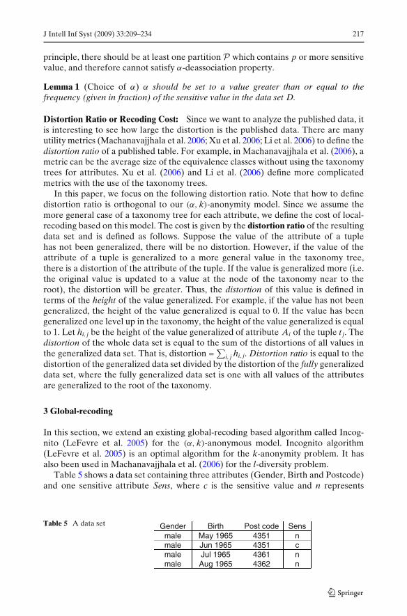
Table 5 shows a data set containing three attributes (Gender, Birth and Postcode)and one sensitive attribute Sens, where c is the sensitive value and n represents

Table 5 A data set Gender Birth Post code Sensmale May 1965 4351 nmale Jun 1965 4351 cmale Jul 1965 4361 nmale Aug 1965 4362 n

218 J Intell Inf Syst (2009) 33:209–234

P4 = {****}

P3 = {4***}

P2 = {43**}

P1 = {435*, 436*}

P0 = {4351, 4361, 4362}

B2 = {*}

B1 = {1965}

B0 = {May 1965, Jun 1965, Jul 1965, Aug 1965}

G0 = {male, female}

G1 = {Person}

(a) (b)

(c)

Fig. 1 Generalization hierarchy

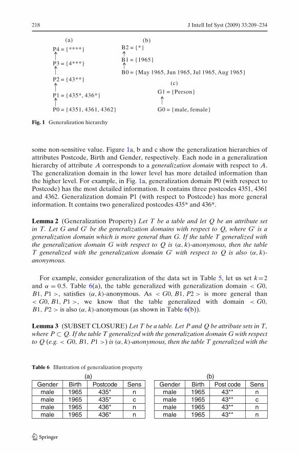
some non-sensitive value. Figure 1a, b and c show the generalization hierarchies ofattributes Postcode, Birth and Gender, respectively. Each node in a generalizationhierarchy of attribute A corresponds to a generalization domain with respect to A.The generalization domain in the lower level has more detailed information thanthe higher level. For example, in Fig. 1a, generalization domain P0 (with respect toPostcode) has the most detailed information. It contains three postcodes 4351, 4361and 4362. Generalization domain P1 (with respect to Postcode) has more generalinformation. It contains two generalized postcodes 435* and 436*.

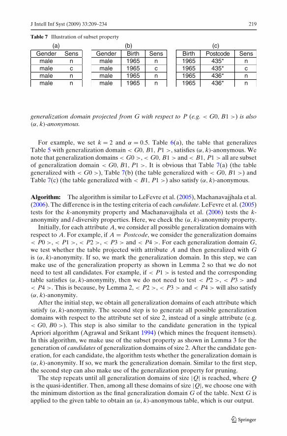
Lemma 2 (Generalization Property) Let T be a table and let Q be an attribute setin T. Let G and G′ be the generalization domains with respect to Q, where G′ is ageneralization domain which is more general than G. If the table T generalized withthe generalization domain G with respect to Q is (α, k)-anonymous, then the tableT generalized with the generalization domain G′ with respect to Q is also (α, k)-anonymous.

For example, consider generalization of the data set in Table 5, let us set k=2and α = 0.5. Table 6(a), the table generalized with generalization domain < G0,

B1, P1 >, satisfies (α, k)-anonymous. As < G0, B1, P2 > is more general than< G0, B1, P1 >, we know that the table generalized with domain < G0,

B1, P2 > is also (α, k)-anonymous (as shown in Table 6(b)).

Lemma 3 (SUBSET CLOSURE) Let T be a table. Let P and Q be attribute sets in T,where P ⊂ Q. If the table T generalized with the generalization domain G with respectto Q (e.g. < G0, B1, P1 >) is (α, k)-anonymous, then the table T generalized with the

Table 6 Illustration of generalization property

(a) (b)Gender Birth Postcode Sens

male 1965 435* nmale 1965 435* cmale 1965 436* nmale 1965 436* n

Gender Birth Post code Sensmale 1965 43** nmale 1965 43** cmale 1965 43** nmale 1965 43** n

J Intell Inf Syst (2009) 33:209–234 219

Table 7 Illustration of subset property

(a) (b) (c)Gender Sens

male nmale cmale nmale n

Gender Birth Sensmale 1965 nmale 1965 cmale 1965 nmale 1965 n

Birth Postcode Sens1965 435* n1965 435* c1965 436* n1965 436* n

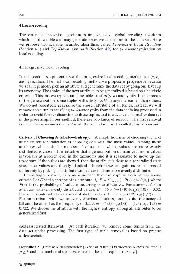
generalization domain projected from G with respect to P (e.g. < G0, B1 >) is also(α, k)-anonymous.

For example, we set k = 2 and α = 0.5. Table 6(a), the table that generalizesTable 5 with generalization domain < G0, B1, P1 >, satisfies (α, k)-anonymous. Wenote that generalization domains < G0 >, < G0, B1 > and < B1, P1 > all are subsetof generalization domain < G0, B1, P1 >. It is obvious that Table 7(a) (the tablegeneralized with < G0 >), Table 7(b) (the table generalized with < G0, B1 >) andTable 7(c) (the table generalized with < B1, P1 >) also satisfy (α, k)-anonymous.

Algorithm: The algorithm is similar to LeFevre et al. (2005), Machanavajjhala et al.(2006). The difference is in the testing criteria of each candidate. LeFevre et al. (2005)tests for the k-anonymity property and Machanavajjhala et al. (2006) tests the k-anonymity and l-diversity properties. Here, we check the (α, k)-anonymity property.

Initially, for each attribute A, we consider all possible generalization domains withrespect to A. For example, if A = Postcode, we consider the generalization domains< P0 >, < P1 >, < P2 >, < P3 > and < P4 >. For each generalization domain G,we test whether the table projected with attribute A and then generalized with Gis (α, k)-anonymity. If so, we mark the generalization domain. In this step, we canmake use of the generalization property as shown in Lemma 2 so that we do notneed to test all candidates. For example, if < P1 > is tested and the correspondingtable satisfies (α, k)-anonymity, then we do not need to test < P2 >, < P3 > and< P4 >. This is because, by Lemma 2, < P2 >, < P3 > and < P4 > will also satisfy(α, k)-anonymity.

After the initial step, we obtain all generalization domains of each attribute whichsatisfy (α, k)-anonymity. The second step is to generate all possible generalizationdomains with respect to the attribute set of size 2, instead of a single attribute (e.g.< G0, B0 >). This step is also similar to the candidate generation in the typicalApriori algorithm (Agrawal and Srikant 1994) (which mines the frequent itemsets).In this algorithm, we make use of the subset property as shown in Lemma 3 for thegeneration of candidates of generalization domains of size 2. After the candidate gen-eration, for each candidate, the algorithm tests whether the generalization domain is(α, k)-anonymity. If so, we mark the generalization domain. Similar to the first step,the second step can also make use of the generalization property for pruning.

The step repeats until all generalization domains of size |Q| is reached, where Qis the quasi-identifier. Then, among all these domains of size |Q|, we choose one withthe minimum distortion as the final generalization domain G of the table. Next G isapplied to the given table to obtain an (α, k)-anonymous table, which is our output.

220 J Intell Inf Syst (2009) 33:209–234

4 Local-recoding

The extended Incognito algorithm is an exhaustive global recoding algorithmwhich is not scalable and may generate excessive distortions to the data set. Herewe propose two scalable heuristic algorithms called Progressive Local Recoding(Section 4.1) and Top-Down Approach (Section 4.2) for (α, k)-anonymization bylocal recoding.

4.1 Progressive local recoding

In this section, we present a scalable progressive local-recoding method for (α, k)-anonymization. The first local-recoding method we propose is progressive becausewe shall repeatedly pick an attribute and generalize the data set by going one level upits taxonomy. The choice of the next attribute to be generalized is based on a heuristiccriterion. This process repeats until the table satisfies (α, k)-anonymity. In the processof the generalization, some tuples will satisfy (α, k)-anonymity earlier than others.We do not repeatedly generalize the chosen attribute of all tuples. Instead, we willremove some tuples satisfying (α, k)-anonymity from the data set being processed inorder to avoid further distortion to these tuples, and to advance to a smaller data setin the processing. In our method, there are two kinds of removal. The first removalis called α-deassociated removal while the second removal is called further removal.

Criteria of Choosing Attribute—Entropy: A simple heuristic of choosing the nextattribute for generalization is choosing one with the most values. Among thoseattributes with a similar number of values, one whose values are more evenlydistributed is chosen. It is intuitive that a generalization domain with more valuesis typically at a lower level in the taxonomy and it is reasonable to move up thetaxonomy. If the values are skewed, then the attribute is close to a generalized statesince most values are already identical. Therefore we can gain more in terms ofuniformity by picking an attribute with values that are more evenly distributed.

Interestingly, entropy is a measurement that can capture both of the abovecriteria. Let E be the entropy of an attribute Ai. E = ∑

∀v∈Ai[−P(v) log2 P(v)], where

P(v) is the probability of value v occurring in attribute Ai. For example, for anattribute with ten evenly distributed values, E = 10 × (−(1/10) log2(1/10)) = 3.32.For an attribute with two evenly distributed values, E = 2 × (−(1/2) log2(1/2)) = 1.For an attribute with two unevenly distributed values, one has the frequency of0.8 and the other has the frequency of 0.2. E = −(4/5) log2(4/5) − (1/5) log2(1/5) =0.722. We choose the attribute with the highest entropy among all attributes to begeneralized first.

α-Deassociated Removal: At each iteration, we remove some tuples from thedata set under processing. The first type of tuple removal is based on preciseα-deassociation.

Definition 8 (Precise α-deassociation) A set of p tuples is precisely α-deassociated ifp ≥ k and the number of sensitive values in the set is equal to �α × p�.

J Intell Inf Syst (2009) 33:209–234 221

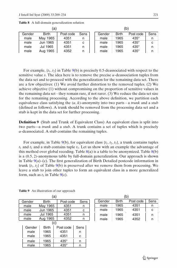
Table 8 A full-domain generalization solution

(a) (b)Gender Birth Post code Sens

male May 1965 4351 nmale Jun 1965 4351 cmale Jul 1965 4351 nmale Aug 1965 4352 n

Gender Birth Post code Sensmale 1965 435* nmale 1965 435* cmale 1965 435* nmale 1965 435* n

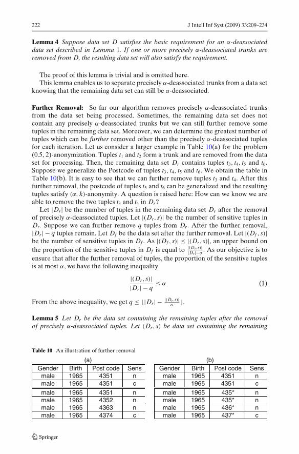
For example, {t1, t2} in Table 9(b) is precisely 0.5-deassociated with respect to thesensitive value s. The idea here is to remove the precise α-deassociation tuples fromthe data set and to proceed with the generalization for the remaining data set. Thereare a few objectives: (1) We avoid further distortion to the removed tuples. (2) Weachieve objective (1) without compromising on the proportion of sensitive values inthe remaining data set - they remain rare, if not rarer. (3) We reduce the data set sizefor the remaining processing. According to the above definition, we partition eachequivalence class satisfying the (α, k)-anonymity into two parts - a trunk and a stub(defined as follows). A trunk should be removed from the processing data set and astub is kept in the data set for further processing.

Definition 9 (Stub and Trunk of Equivalent Class) An equivalent class is split intotwo parts—a trunk and a stub. A trunk contains a set of tuples which is preciselyα-deassociated. A stub contains the remaining tuples.

For example, in Table 9(b), for equivalent class {t1, t2, t3}, a trunk contains tuplest1 and t2 and a stub contains tuple t3. Let us show with an example the advantage ofthis method over global recoding. Table 8(a) is a table to be anonymized. Table 8(b)is a (0.5, 2)-anonymous table by full-domain generalization. Our approach is shownin Table 9(a)–(c). The first generalization of Birth Detailed postcode information intrunk {t1, t2} of Table 9(b) is preserved after we remove them from processing. Weleave a stub to join other tuples to form an equivalent class in a more generalizedform, such as t3 in Table 9(c).

Table 9 An illustration of our approach

(a) (b)Gender Birth Post code Sens

male May 1965 4351 nmale Jun 1965 4351 cmale Jul 1965 4351 nmale Aug 1965 4352 n

Gender Birth Post code Sensmale 1965 4351 nmale 1965 4351 c

male 1965 4351 nmale 1965 4352 n

(c)Gender Birth Post code Sens

male 1965 4351 nmale 1965 4351 c

male 1965 435* nmale 1965 435* n

222 J Intell Inf Syst (2009) 33:209–234

Lemma 4 Suppose data set D satisfies the basic requirement for an α-deassociateddata set described in Lemma 1. If one or more precisely α-deassociated trunks areremoved from D, the resulting data set will also satisfy the requirement.

The proof of this lemma is trivial and is omitted here.This lemma enables us to separate precisely α-deassociated trunks from a data set

knowing that the remaining data set can still be α-deassociated.

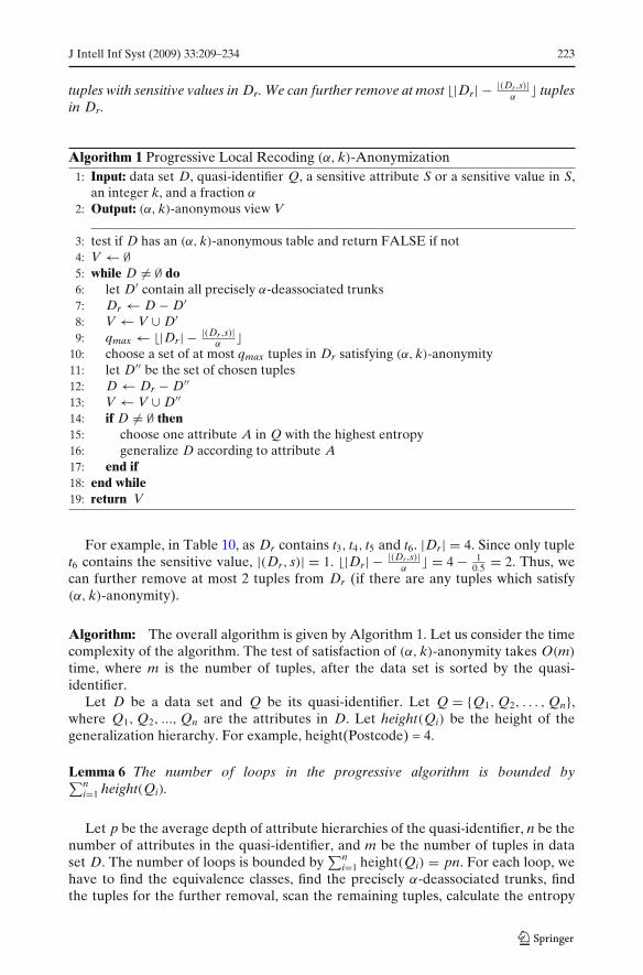
Further Removal: So far our algorithm removes precisely α-deassociated trunksfrom the data set being processed. Sometimes, the remaining data set does notcontain any precisely α-deassociated trunks but we can still further remove sometuples in the remaining data set. Moreover, we can determine the greatest number oftuples which can be further removed other than the precisely α-deassociated tuplesfor each iteration. Let us consider a larger example in Table 10(a) for the problem(0.5, 2)-anonymization. Tuples t1 and t2 form a trunk and are removed from the dataset for processing. Then, the remaining data set Dr contains tuples t3, t4, t5 and t6.Suppose we generalize the Postcode of tuples t3, t4, t5 and t6. We obtain the table inTable 10(b). It is easy to see that we can further remove tuples t3 and t4. After thisfurther removal, the postcode of tuples t5 and t6 can be generalized and the resultingtuples satisfy (α, k)-anonymity. A question is raised here: How can we know we areable to remove the two tuples t3 and t4 in Dr?

Let |Dr| be the number of tuples in the remaining data set Dr after the removalof precisely α-deassociated tuples. Let |(Dr, s)| be the number of sensitive tuples inDr. Suppose we can further remove q tuples from Dr. After the further removal,|Dr| − q tuples remain. Let Df be the data set after the further removal. Let |(Df , s)|be the number of sensitive tuples in Df . As |(Df , s)| ≤ |(Dr, s)|, an upper bound onthe proportion of the sensitive tuples in Df is equal to |(Dr,s)|

|Dr |−q . As our objective is toensure that after the further removal of tuples, the proportion of the sensitive tuplesis at most α, we have the following inequality

|(Dr, s)||Dr| − q

≤ α (1)

From the above inequality, we get q ≤ �|Dr| − |(Dr,s)|α

�.

Lemma 5 Let Dr be the data set containing the remaining tuples after the removalof precisely α-deassociated tuples. Let (Dr, s) be data set containing the remaining

Table 10 An illustration of further removal

(a) (b)Gender Birth Post code Sens

male 1965 4351 nmale 1965 4351 c

male 1965 4351 nmale 1965 4352 nmale 1965 4363 nmale 1965 4374 c

Gender Birth Post code Sensmale 1965 4351 nmale 1965 4351 c

male 1965 435* nmale 1965 435* nmale 1965 436* nmale 1965 437* c

J Intell Inf Syst (2009) 33:209–234 223

tuples with sensitive values in Dr. We can further remove at most �|Dr| − |(Dr,s)|α

� tuplesin Dr.

Algorithm 1 Progressive Local Recoding (α, k)-Anonymization1: Input: data set D, quasi-identifier Q, a sensitive attribute S or a sensitive value in S,

an integer k, and a fraction α

2: Output: (α, k)-anonymous view V

3: test if D has an (α, k)-anonymous table and return FALSE if not4: V ← ∅5: while D �= ∅ do6: let D′ contain all precisely α-deassociated trunks7: Dr ← D − D′8: V ← V ∪ D′9: qmax ← �|Dr| − |(Dr,s)|

α�

10: choose a set of at most qmax tuples in Dr satisfying (α, k)-anonymity11: let D′′ be the set of chosen tuples12: D ← Dr − D′′13: V ← V ∪ D′′14: if D �= ∅ then15: choose one attribute A in Q with the highest entropy16: generalize D according to attribute A17: end if18: end while19: return V

For example, in Table 10, as Dr contains t3, t4, t5 and t6. |Dr| = 4. Since only tuplet6 contains the sensitive value, |(Dr, s)| = 1. �|Dr| − |(Dr,s)|

α� = 4 − 1

0.5 = 2. Thus, wecan further remove at most 2 tuples from Dr (if there are any tuples which satisfy(α, k)-anonymity).

Algorithm: The overall algorithm is given by Algorithm 1. Let us consider the timecomplexity of the algorithm. The test of satisfaction of (α, k)-anonymity takes O(m)

time, where m is the number of tuples, after the data set is sorted by the quasi-identifier.

Let D be a data set and Q be its quasi-identifier. Let Q = {Q1, Q2, . . . , Qn},where Q1, Q2, ..., Qn are the attributes in D. Let height(Qi) be the height of thegeneralization hierarchy. For example, height(Postcode) = 4.

Lemma 6 The number of loops in the progressive algorithm is bounded by∑ni=1 height(Qi).

Let p be the average depth of attribute hierarchies of the quasi-identifier, n be thenumber of attributes in the quasi-identifier, and m be the number of tuples in dataset D. The number of loops is bounded by

∑ni=1 height(Qi) = pn. For each loop, we

have to find the equivalence classes, find the precisely α-deassociated trunks, findthe tuples for the further removal, scan the remaining tuples, calculate the entropy

224 J Intell Inf Syst (2009) 33:209–234

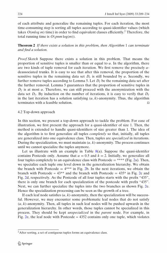
of each attribute and generalize the remaining tuples. For each iteration, the mosttime-consuming step is sorting all tuples according to quasi-identifier values (whichtakes O(mlog m) time) in order to find equivalent classes efficiently.2 Therefore, thetotal running time is O(pnm log(m)).

Theorem 2 If there exists a solution in this problem, then Algorithm 1 can terminateand find a solution.

Proof Sketch Suppose there exists a solution in this problem. That means theproportion of sensitive tuples is smaller than or equal to α. In the algorithm, thereare two kinds of tuple removal for each iteration. We first remove the precisely α-deassociated trunks. It is easy to see that after this removal, the proportion of thesensitive tuples in the remaining data set Dr is still bounded by α. Secondly, wefurther remove tuples according to Lemma 5. Let Df be the remaining data set afterthe further removal. Lemma 5 guarantees that the proportion of sensitive tuples inDf is at most α. Therefore, we can still proceed with the anonymization with thedata set Df . By induction on the number of iterations, it is easy to verify that Df

in the last iteration has a solution satisfying (α, k)-anonymity. Thus, the algorithmterminates with a feasible solution. �

4.2 Top-down approach

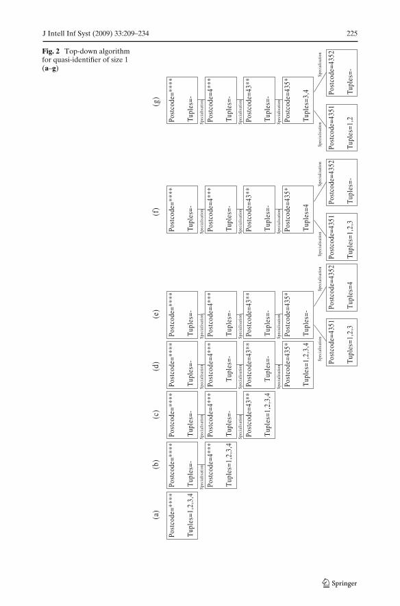
In this section, we present a top-down approach to tackle the problem. For ease ofillustration, we first present the approach for a quasi-identifier of size 1. Then, themethod is extended to handle quasi-identifiers of size greater than 1. The idea ofthe algorithm is to first generalize all tuples completely so that, initially, all tuplesare generalized into one equivalence class. Then, tuples are specialized in iterations.During the specialization, we must maintain (α, k)-anonymity. The process continuesuntil we cannot specialize the tuples anymore.

Let us illustrate with an example in Table 8(a). Suppose the quasi-identifercontains Postcode only. Assume that α = 0.5 and k = 2. Initially, we generalize allfour tuples completely to an equivalence class with Postcode = **** (Fig. 2a). Then,we specialize each tuple one level down in the generalization hierarchy. We obtainthe branch with Postcode = 4*** in Fig. 2b. In the next iterations, we obtain thebranch with Postcode = 43** and the branch with Postcode = 435* in Fig. 2c andFig. 2d, respectively. As the Postcode of all four tuples starts with the prefix “435”,there is only one branch for each specialization of the postcode with prefix “435”.Next, we can further specialize the tuples into the two branches as shown Fig. 2e.Hence the specialization processing can be seen as the growth of a tree.

If each leaf node satisfies (α, k)-anonymity, then the specialization will be success-ful. However, we may encounter some problematic leaf nodes that do not satisfy(α, k)-anonymity. Then, all tuples in such leaf nodes will be pushed upwards in thegeneralization hierarchy. In other words, those tuples cannot be specialized in thisprocess. They should be kept unspecialized in the parent node. For example, inFig. 2e, the leaf node with Postcode = 4352 contains only one tuple, which violates

2After sorting, a set of contiguous tuples forms an equivalence class.

J Intell Inf Syst (2009) 33:209–234 225

Fig. 2 Top-down algorithmfor quasi-identifier of size 1(a–g)

Post

code

=***

*

Tup

les=

1,2,

3,4

Post

code

=***

*

Tup

les=

-

Post

code

=4**

*

Tup

les=

1,2,

3,4

Spec

ialis

atio

n

Post

code

=***

*

Tup

les=

-

Post

code

=4**

*

Tup

les=

-

Spec

ialis

atio

n

Post

code

=43*

*

Tup

les=

1,2,

3,4

Spec

ialis

atio

n

Post

code

=***

*

Tup

les=

-

Post

code

=4**

*

Tup

les=

-

Spec

ialis

atio

n

Post

code

=43*

*

Tup

les=

-

Spec

ialis

atio

n

Post

code

=435

*

Tup

les=

1,2,

3,4

Spec

ialis

atio

n

Post

code

=***

*

Tup

les=

-

Post

code

=4**

*

Tup

les=

-

Spec

ialis

atio

n

Post

code

=43*

*

Tup

les=

-

Spec

ialis

atio

n

Post

code

=435

*

Tup

les=

-

Spec

ialis

atio

n

Post

code

=435

1

Tup

les=

1,2,

3

Spec

ialis

atio

n

Post

code

=435

2

Tup

les=

4

Spec

ialis

atio

n

Post

code

=***

*

Tupl

es=-

Post

code

=4**

*

Tupl

es=-

Spec

ialis

atio

n

Post

code

=43*

*

Tup

les=

-

Spec

ialis

atio

n

Post

code

=435

*

Tup

les=

4

Spec

ialis

atio

n

Post

code

=435

1

Tup

les=

1,2,

3

Spec

ialis

atio

n

Post

code

=435

2

Tup

les=

-

Spec

ialis

atio

n

Post

code

=***

*

Tupl

es=-

Post

code

=4**

*

Tupl

es=-

Spec

ialis

atio

n

Post

code

=43*

*

Tupl

es=-

Spec

ialis

atio

n

Post

code

=435

*

Tupl

es=3

,4

Spec

ialis

atio

n

Post

code

=435

1

Tupl

es=1

,2

Spec

ialis

atio

n

Post

code

=435

2

Tupl

es=-Sp

ecia

lisat

ion

(a)

(b)

(c)

(d)

(e)

(f)

(g)

226 J Intell Inf Syst (2009) 33:209–234

Table 11 Projected table withquasi-identifier = postcode: (a)Original table and (b)Generalized table

(a) (b)No Post code Sens1 4351 n2 4351 c3 4351 n4 4352 n

No Post code Sens1 4351 n2 4351 c3 435* n4 435* n

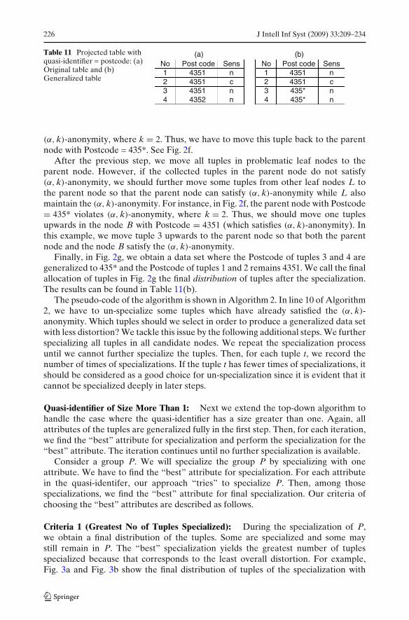
(α, k)-anonymity, where k = 2. Thus, we have to move this tuple back to the parentnode with Postcode = 435*. See Fig. 2f.

After the previous step, we move all tuples in problematic leaf nodes to theparent node. However, if the collected tuples in the parent node do not satisfy(α, k)-anonymity, we should further move some tuples from other leaf nodes L tothe parent node so that the parent node can satisfy (α, k)-anonymity while L alsomaintain the (α, k)-anonymity. For instance, in Fig. 2f, the parent node with Postcode= 435* violates (α, k)-anonymity, where k = 2. Thus, we should move one tuplesupwards in the node B with Postcode = 4351 (which satisfies (α, k)-anonymity). Inthis example, we move tuple 3 upwards to the parent node so that both the parentnode and the node B satisfy the (α, k)-anonymity.

Finally, in Fig. 2g, we obtain a data set where the Postcode of tuples 3 and 4 aregeneralized to 435* and the Postcode of tuples 1 and 2 remains 4351. We call the finalallocation of tuples in Fig. 2g the final distribution of tuples after the specialization.The results can be found in Table 11(b).

The pseudo-code of the algorithm is shown in Algorithm 2. In line 10 of Algorithm2, we have to un-specialize some tuples which have already satisfied the (α, k)-anonymity. Which tuples should we select in order to produce a generalized data setwith less distortion? We tackle this issue by the following additional steps. We furtherspecializing all tuples in all candidate nodes. We repeat the specialization processuntil we cannot further specialize the tuples. Then, for each tuple t, we record thenumber of times of specializations. If the tuple t has fewer times of specializations, itshould be considered as a good choice for un-specialization since it is evident that itcannot be specialized deeply in later steps.

Quasi-identifier of Size More Than 1: Next we extend the top-down algorithm tohandle the case where the quasi-identifier has a size greater than one. Again, allattributes of the tuples are generalized fully in the first step. Then, for each iteration,we find the “best” attribute for specialization and perform the specialization for the“best” attribute. The iteration continues until no further specialization is available.

Consider a group P. We will specialize the group P by specializing with oneattribute. We have to find the “best” attribute for specialization. For each attributein the quasi-identifer, our approach “tries” to specialize P. Then, among thosespecializations, we find the “best” attribute for final specialization. Our criteria ofchoosing the “best” attributes are described as follows.

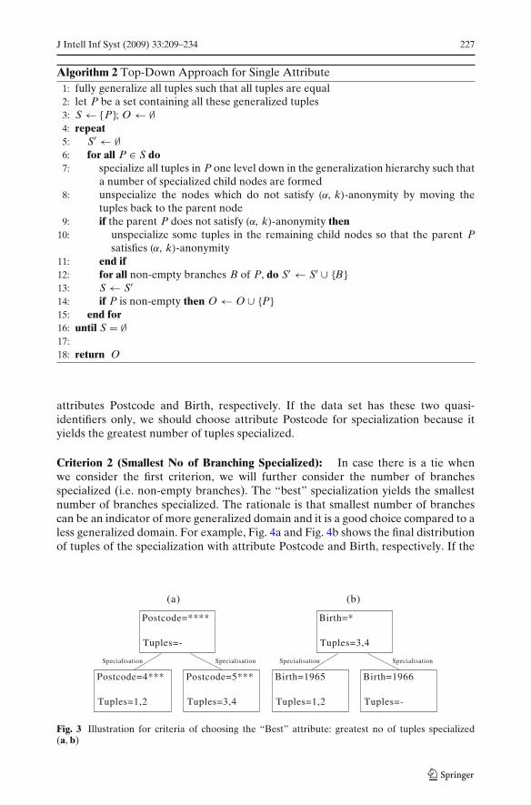
Criteria 1 (Greatest No of Tuples Specialized): During the specialization of P,we obtain a final distribution of the tuples. Some are specialized and some maystill remain in P. The “best” specialization yields the greatest number of tuplesspecialized because that corresponds to the least overall distortion. For example,Fig. 3a and Fig. 3b show the final distribution of tuples of the specialization with

J Intell Inf Syst (2009) 33:209–234 227

Algorithm 2 Top-Down Approach for Single Attribute1: fully generalize all tuples such that all tuples are equal2: let P be a set containing all these generalized tuples3: S {P}; O4: repeat5: S6: for all P S do7: specialize all tuples in P one level down in the generalization hierarchy such that

a number of specialized child nodes are formed8: unspecialize the nodes which do not satisfy ( , k)-anonymity by moving the

tuples back to the parent node9: if the parent P does not satisfy ( , k)-anonymity then

10: unspecialize some tuples in the remaining child nodes so that the parent Psatisfies ( , k)-anonymity

11: end if12: for all non-empty branches B of P, do S S {B}13: S S14: if P is non-empty then O O {P}15: end for16: until S17:18: return O

attributes Postcode and Birth, respectively. If the data set has these two quasi-identifiers only, we should choose attribute Postcode for specialization because ityields the greatest number of tuples specialized.

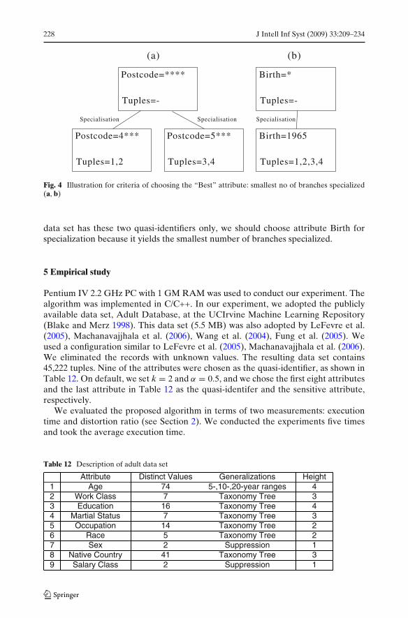
Criterion 2 (Smallest No of Branching Specialized): In case there is a tie whenwe consider the first criterion, we will further consider the number of branchesspecialized (i.e. non-empty branches). The “best” specialization yields the smallestnumber of branches specialized. The rationale is that smallest number of branchescan be an indicator of more generalized domain and it is a good choice compared to aless generalized domain. For example, Fig. 4a and Fig. 4b shows the final distributionof tuples of the specialization with attribute Postcode and Birth, respectively. If the

Postcode=****

Tuples=-

Postcode=4***

Tuples=1,2

Specialisation

Postcode=5***

Tuples=3,4

Specialisation

Birth=*

Tuples=3,4

Birth=1965

Tuples=1,2

Specialisation

Birth=1966

Tuples=-

Specialisation

(a) (b)

Fig. 3 Illustration for criteria of choosing the “Best” attribute: greatest no of tuples specialized(a, b)

228 J Intell Inf Syst (2009) 33:209–234

Postcode=****

Tuples=-

Postcode=4***

Tuples=1,2

Specialisation

Postcode=5***

Tuples=3,4

Specialisation

Birth=*

Tuples=-

Birth=1965

Tuples=1,2,3,4

Specialisation

(a) (b)

Fig. 4 Illustration for criteria of choosing the “Best” attribute: smallest no of branches specialized(a, b)

data set has these two quasi-identifiers only, we should choose attribute Birth forspecialization because it yields the smallest number of branches specialized.

5 Empirical study

Pentium IV 2.2 GHz PC with 1 GM RAM was used to conduct our experiment. Thealgorithm was implemented in C/C++. In our experiment, we adopted the publiclyavailable data set, Adult Database, at the UCIrvine Machine Learning Repository(Blake and Merz 1998). This data set (5.5 MB) was also adopted by LeFevre et al.(2005), Machanavajjhala et al. (2006), Wang et al. (2004), Fung et al. (2005). Weused a configuration similar to LeFevre et al. (2005), Machanavajjhala et al. (2006).We eliminated the records with unknown values. The resulting data set contains45,222 tuples. Nine of the attributes were chosen as the quasi-identifier, as shown inTable 12. On default, we set k = 2 and α = 0.5, and we chose the first eight attributesand the last attribute in Table 12 as the quasi-identifer and the sensitive attribute,respectively.

We evaluated the proposed algorithm in terms of two measurements: executiontime and distortion ratio (see Section 2). We conducted the experiments five timesand took the average execution time.

Table 12 Description of adult data set

Attribute Distinct Values Generalizations Height1 Age 74 5-,10-,20-year ranges 42 Work Class 7 Taxonomy Tree 33 Education 16 Taxonomy Tree 44 Martial Status 7 Taxonomy Tree 35 Occupation 14 Taxonomy Tree 26 Race 5 Taxonomy Tree 27 Sex 2 Suppression 18 Native Country 41 Taxonomy Tree 39 Salary Class 2 Suppression 1

J Intell Inf Syst (2009) 33:209–234 229

We denote the proposed algorithms by Progressive, Top Down and eIncognito.eIncognito denotes the extended Incognito algorithm while Progressive and TopDown denote the local-recoding based progressive approach and the local-recodingbased top-down approach, respectively.

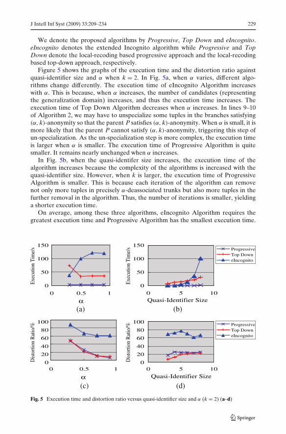
Figure 5 shows the graphs of the execution time and the distortion ratio againstquasi-identifier size and α when k = 2. In Fig. 5a, when α varies, different algo-rithms change differently. The execution time of eIncognito Algorithm increaseswith α. This is because, when α increases, the number of candidates (representingthe generalization domain) increases, and thus the execution time increases. Theexecution time of Top Down Algorithm decreases when α increases. In lines 9–10of Algorithm 2, we may have to unspecialize some tuples in the branches satisfying(α, k)-anonymity so that the parent P satisfies (α, k)-anonymity. When α is small, it ismore likely that the parent P cannot satisfy (α, k)-anonymity, triggering this step ofun-specialization. As the un-specialization step is more complex, the execution timeis larger when α is smaller. The execution time of Progressive Algorithm is quitesmaller. It remains nearly unchanged when α increases.

In Fig. 5b, when the quasi-identifer size increases, the execution time of thealgorithm increases because the complexity of the algorithms is increased with thequasi-identifier size. However, when k is larger, the execution time of ProgressiveAlgorithm is smaller. This is because each iteration of the algorithm can removenot only more tuples in precisely α-deassociated trunks but also more tuples in thefurther removal in the algorithm. Thus, the number of iterations is smaller, yieldinga shorter execution time.

On average, among these three algorithms, eIncognito Algorithm requires thegreatest execution time and Progressive Algorithm has the smallest execution time.

(a) (b)

(c) (d)

Fig. 5 Execution time and distortion ratio versus quasi-identifier size and α (k = 2) (a–d)

230 J Intell Inf Syst (2009) 33:209–234

This shows that eIncognito performs much slower compared with local-recodingbased algorithms.

In Fig. 5c, when α increases, the distortion ratio decreases. Intuitively, if α isgreater, there is less requirement of α-deassociation, yielding fewer operations ofgeneralization of the values in the data set. Thus, the distortion ratio is smaller.

In Fig. 5d, it is easy to see why the distortion ratio increases with the quasi-identifier size. When the quasi-identifier contains more attributes, there is morechance that the quasi-identifier of two tuples are different. In other words, there ismore chance that the tuples will be generalized. Thus, the distortion ratio is greater.When k is larger, it is also obvious that the distortion ratio is greater because it is lesslikely that the quasi-identifer of two tuples are equal.

On average, the local-recoding based algorithms (Progressive Algorithm and TopDown Algorithm) result in about 3 times smaller distortion ratio compared witheIncognito Algorithm. Also, the Progressive Algorithm and Top Down Algorithmgenerate similar distortion ratio.

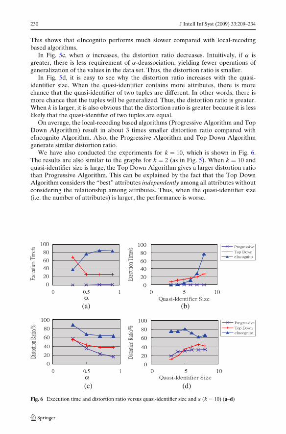
We have also conducted the experiments for k = 10, which is shown in Fig. 6.The results are also similar to the graphs for k = 2 (as in Fig. 5). When k = 10 andquasi-identifier size is large, the Top Down Algorithm gives a larger distortion ratiothan Progressive Algorithm. This can be explained by the fact that the Top DownAlgorithm considers the “best” attributes independently among all attributes withoutconsidering the relationship among attributes. Thus, when the quasi-identifier size(i.e. the number of attributes) is larger, the performance is worse.

(a) (b)

(c) (d)

Fig. 6 Execution time and distortion ratio versus quasi-identifier size and α (k = 10) (a–d)

J Intell Inf Syst (2009) 33:209–234 231

6 General (α, k)-anonymity model

In this section, we will extend the simple (α, k)-model to two different cases: (1)multiple sensitive values in a single sensitive attribute (Section 6.1) and (2) multiplesensitive values in multiple sensitive attributes (Section 6.2).

6.1 Multiple sensitive values

When there are two or more sensitive values and they are rare cases in a data set(e.g. HIV and prostate cancer). We may combine them into one combined sensitiveclass and the simple (α, k)-anonymity model is applicable. The inference confidenceto each individual sensitive value is smaller than or equal to the confidence to thecombined value, which is controlled by α.

Next we consider the case when all values in an attribute are sensitive and requireprotection. It is possible to have an (α, k)-anonymity model to protect a sensitiveattribute when the attribute contains many values and no single value dominatesthe attribute (which will be explained later). The salary attribute in employer tableis an example. When each equivalent class contains three salary scales with evendistribution, we have about 33% confidence to infer the salary scale of an individualin the equivalent class.

Definition 10 (α-rare) Given an equivalence class E, an attribute X and an attributevalue x ∈ X. Let (E, x) be the set of tuples containing x in E and α be a user-specifiedthreshold, where 0 ≤ α ≤ 1. Equivalence class E is α-rare with respect to attribute setX if the proportion of every attribute value of X in the data set is not greater than α,i.e. |(E, x)|/|E| ≤ α for x ∈ X.

For example, in Table 3, if X = Illness, equivalent class {t3, t4} is 0.5-rare because“flu” and “fever” occur evenly in the equivalent class. If every equivalent class isα-rare in the class, the data set is called α-deassociated.

Definition 11 (General α-deassociation property) Given a data set D, an attributeset Q and a sensitive class attribute S. Let α be a user-specified threshold, where0 ≤ α ≤ 1. Data set D is said to satisfy general α-deassociation with respect to anattribute set Q and a sensitive attribute S if, for any equivalent classes E ⊂ D, E isα-rare with respect to S.

For example, Table 3 is 0.5-deassociated since all three equivalent classes, {t1, t6},{t2, t5} and {t3, t4}, are 0.5-rare with respect to attribute set Illness. When a data set isα-deassociated with respect to a sensitive attribute, it is α-deassociated with respectto every value in the attribute. Therefore, the upper bound of inference confidencefrom the quasi-identifier to the sensitive attribute is α.

Definition 12 (General (α, k)-anonymity) Given an attribute set Q and a sensitiveclass attribute S, a view of a table is said to be a general (α, k)-anonymization of thetable if the view modifies the table such that the view satisfies both k-anonymity andgeneral α-deassociation with respect to an attribute set Q and a sensitive attribute S.

232 J Intell Inf Syst (2009) 33:209–234

The proposed algorithms in Sections 3 and 4 can be extended to the general (α, k)-anonymity model. The global-recoding based algorithm depends on two major prop-erties - the generalization property (Lemma 2) and the subset property (Lemma 3).Both propoerties hold for the general (α, k)-anonymity. Thus, the global-recodingbased algorithm can be extended by modifying the step of testing of candidates withthe general model.

The progressive local-recoding algorithm contains three major components -(1) Criteria of Choosing Attributes, (2) α-Deassociated Removal and (3) FurtherRemoval. (1) As the measurement for the criteria of choosing attribute is basedon the quasi-identifier but no sensitive attribute, this component can still be useddirectly. Although we cannot apply (2), we can continue to use step (3), by modifyingthe bound of the number of removal. Recall that we can further remove at most�|Dr| − |(Dr,s)|

α� (Lemma 5) in the mode for a single sensitive value s. In the general

mode, all sensitive values should satisfy Eq. 1. That is, the formula in Lemma 5becomes �|Dr| − |(Dr,s)|

α� for all s ∈ S, where S is the sensitive attribute. As we make

sure that all the sensitive values in the sensitive attribute should satisfy the general(α, k)-anonymity, we should remove at most mins∈S{�|Dr| − |(Dr,s)|

α�}. After these

modifications, the progressive algorithm can handle the general model.The top-down local-recoding algorithm can also be easily extended to the general

model by modifying the condition when testing the candidates.

6.2 Multiple sensitive attributes

In some cases, the table may contain multiple sensitive attributes. For example, inaddition to attribute Illness, there are some other sensitive attributes like Income inthe table. We can also easily extend our (α, k)-anonymity model in this case. Let Sbe the set of sensitive attributes in the table. We can refine Definition 11 as follows.

Definition 13 (S-General α-deassociation property) Given a data set D, an attributeset Q and a set S of sensitive attributes. Let α be a user-specified threshold, where0 ≤ α ≤ 1. Data set D is said to satisfy S-general α-deassociation with respect to anattribute set Q and a set S if, for each S ∈ S , D satisfies general α-deassociation withrespect to Q and S.

Definition 14 (S-General (α, k)-anonymity) Given an attribute set Q and a set S ofsensitive attributes, a view of a table is said to be a S-general (α, k)-anonymization ofthe table if the view modifies the table such that the view satisfies both k-anonymityand S-general α-deassociation with respect to an attribute set Q and a set S .

Similarly, we can also adapt our algorithms as follows. Since the generalizationproperty and the subset property hold for the S-general (α, k)-anonymity, we canmodify the step of testing of candidates with this general model.

Similar to Section 6.1, in the progressive local-recoding algorithm, the first stepfor “Criteria of Choosing Attributes” can still be used. For the third step, we shouldremove at most mins∈S and S∈S{�|Dr| − |(Dr,s)|

α�}.

Similarly, the top-down local-recoding algorithm can also be easily extended tothe general model by modifying the condition when testing the candidates.

J Intell Inf Syst (2009) 33:209–234 233

7 Conclusion

The k-anonymity model protects identification information, but does not protectsensitive relationships in a data set. In this paper, we propose the (α, k)-anonymitymodel to protect both identifications and relationships in data. We discuss theproperties of the model. We prove that achieving optimal (α, k)-anonymity bylocal recoding is NP-hard. We present an optimal global-recoding method andtwo efficient local-encoding based algorithms to transform a data set to satisfy(α, k)-anonymity property. The experiment shows that, on average, the two local-encoding based algorithms performs about 4 times faster and gives about 3 times lessdistortions of the data set compared with the global-recoding algorithm.

Acknowledgements We are grateful to the anonymous reviewers for their constructive commentson this paper. This research was supported in part by HKSAR RGC Direct Allocation GrantDAG08/09.EG01 to Raymond Chi-Wing Wong, This research was supported by ARC discoverygrant DP0774450 to Jiuyong Li.

References

Aggarwal, G., Feder, T., Kenthapadi, K., Motwani, R., Panigrahy, R., Thomas, D., et al. (2005).Anonymizing tables. In ICDT (pp. 246–258).

Agrawal, D., & Aggarwal, C. C. (2001). On the design and quantification of privacy preservingdata mining algorithms. In PODS ’01: Proceedings of the twentieth ACM SIGMOD-SIGACT-SIGART symposium on Principles of database systems (pp. 247–255). New York: ACM.

Agrawal, R., & Srikant, R. (1994). Fast algorithms for mining association rules. In VLDB.Agrawal, R., & Srikant, R. (2000). Privacy-preserving data mining. In Proc. of the ACM SIGMOD

conference on management of data (pp. 439–450). New York: ACM.Bayardo, R., & Agrawal, R. (2005). Data privacy through optimal k-anonymization. In ICDE

(pp. 217–228).Blake, E. K. C., & Merz, C. J. (1998). UCI repository of machine learning databases.

http://www.ics.uci.edu/∼mlearn/MLRepository.html.Bu, Y., Fu, A. W.-C., Wong, R. C.-W., Chen, L., & Li, J. (2008). Privacy preserving serial data

publishing by role composition. In VLDB.Cox, L. (1980). Suppression methodology and statistical disclosure control. Journal of the American

Statistical Association, 75, 377–385.Fayyad, U. M., & Irani, K. B. (1993). Multi-interval discretization of continuous-valued attributes for

classification learning. In Proceedings of the thirteenth international joint conference on artificialintelligence (IJCAI-93) (pp. 1022–1027). San Francisco: Morgan Kaufmann.

Fung, B. C. M., Wang, K., & Yu, P. S. (2005). Top-down specialization for information and privacypreservation. In ICDE (pp. 205–216).

Holyer, I. (1981). The np-completeness of some edge-partition problems. SIAM Journal on Comput-ing, 10(4), 713–717.

Hundepool, A. (2004). The argus software in the casc-project: Casc project international workshop.In Privacy in statistical databases. Lecture notes in computer science (Vol. 3050, pp. 323–335).Barcelona: Springer.

Hundepool, A., & Willenborg, L. (1996). μ-and τ - argus: Software for statistical disclosure control.In Third international seminar on statsitcal confidentiality, Bled.

Iyengar, V. S. (2002). Transforming data to satisfy privacy constraints. In KDD ’02: Proceedingsof the eighth ACM SIGKDD international conference on Knowledge discovery and data mining(pp. 279–288).

LeFevre, K., DeWitt, D. J., & Ramakrishnan, R. (2005). Incognito: Efficient full-domaink-anonymity. In SIGMOD conference (pp. 49–60).

Li, J., Wong, R. C.-W., Fu, A. W.-C., & Pei, J. (2006). Achieving k-anonymity by clustering inattribute hierarchical structures. In DaWaK.

Li, N., & Li, T. (2007). t-closeness: Privacy beyond k-anonymity and l-diversity. In ICDE.

234 J Intell Inf Syst (2009) 33:209–234

Machanavajjhala, A., Gehrke, J., & Kifer, D. (2006). l-diversity: Privacy beyond k-anonymity. InICDE06.

Meyerson, A., & Williams, R. (2004). On the complexity of optimal k-anonymity. In PODS(pp. 223–228).

Rizvi, S., & Haritsa, J. (2002). Maintaining data privacy in association rule mining. In Proceedings ofthe 28th conference on very large data base (VLDB02) (pp. 682–693). VLDB Endowment.

Samarati, P. (2001). Protecting respondents’ identities in microdata release. IEEE Transactions onKnowledge and Data Engineering, 13(6), 1010–1027.

Sweeney, L. (2002a). Achieving k-anonymity privacy protection using generalization and suppres-sion. International Journal on Uncertainty, Fuzziness and Knowldege Based Systems, 10(5),571–588.

Sweeney, L. (2002b). k-anonymity: A model for protecting privacy. International Journal on Uncer-tainty, Fuzziness and Knowldeg Based Systems, 10(5), 557–570.

Verykios, V. S., Elmagarmid, A. K., Bertino, E., Saygin, Y., & Dasseni, E. (2004). Association rulehiding. IEEE Transactions on Knowledge and Data Engineering, 16(4), 434–447.

Wang, K., Fung, B. C. M., & Yu, P. S. (2005). Template-based privacy preservation in classificationproblems. In ICDM05.

Wang, K., Fung, B., & Yu, P. (2007). Handicapping attacker’s confidence: An alternative tok-anonymization. Knowledge and Information Systems: An International Journal, 11(3), 345–368.

Wang, K., Yu, P. S., & Chakraborty, S. (2004). Bottom-up generalization: A data mining solution toprivacy protection. In ICDM (pp. 249–256).

Willenborg, L., & de Waal, T. (1996). Statistical disclosure control in practice. Lecture Notes inStatistics, 111.

Xiao, X., & Tao, Y. (2006). Personalized privacy preservation. In SIGMOD.Xiao, X., & Tao, Y. (2007). m-invariance: Towards privacy preserving re-publication of dynamic

datasets. In SIGMOD.Xu, J., Wang, W., Pei, J., Wang, X., Shi, B., & Fu, A. (2006). Utility-based anonymization using local

recoding. In KDD.