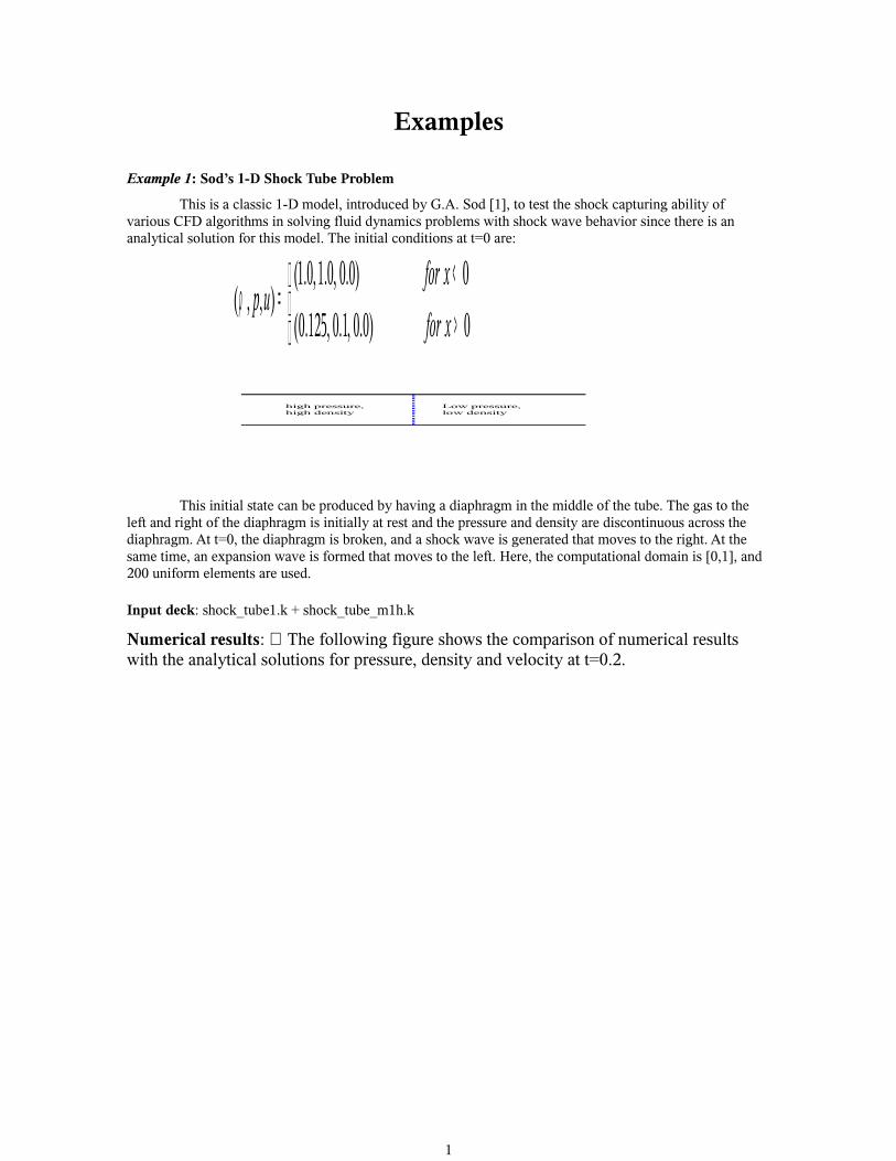
Examples

Example 1: Sod’s 1-D Shock Tube Problem

This is a classic 1-D model, introduced by G.A. Sod [1], to test the shock capturing ability of various CFD algorithms in solving fluid dynamics problems with shock wave behavior since there is an analytical solution for this model. The initial conditions at t=0 are:

><

=0)0.0,1.0,125.0(

0)0.0,0.1,0.1(),,(

xfor

xforupρ

Low pressure, low density

high pressure, high density

This initial state can be produced by having a diaphragm in the middle of the tube. The gas to the left and right of the diaphragm is initially at rest and the pressure and density are discontinuous across the diaphragm. At t=0, the diaphragm is broken, and a shock wave is generated that moves to the right. At the same time, an expansion wave is formed that moves to the left. Here, the computational domain is [0,1], and 200 uniform elements are used.

Input deck: shock_tube1.k + shock_tube_m1h.k

Numerical results: The following figure shows the comparison of numerical results with the analytical solutions for pressure, density and velocity at t=0.2.

1

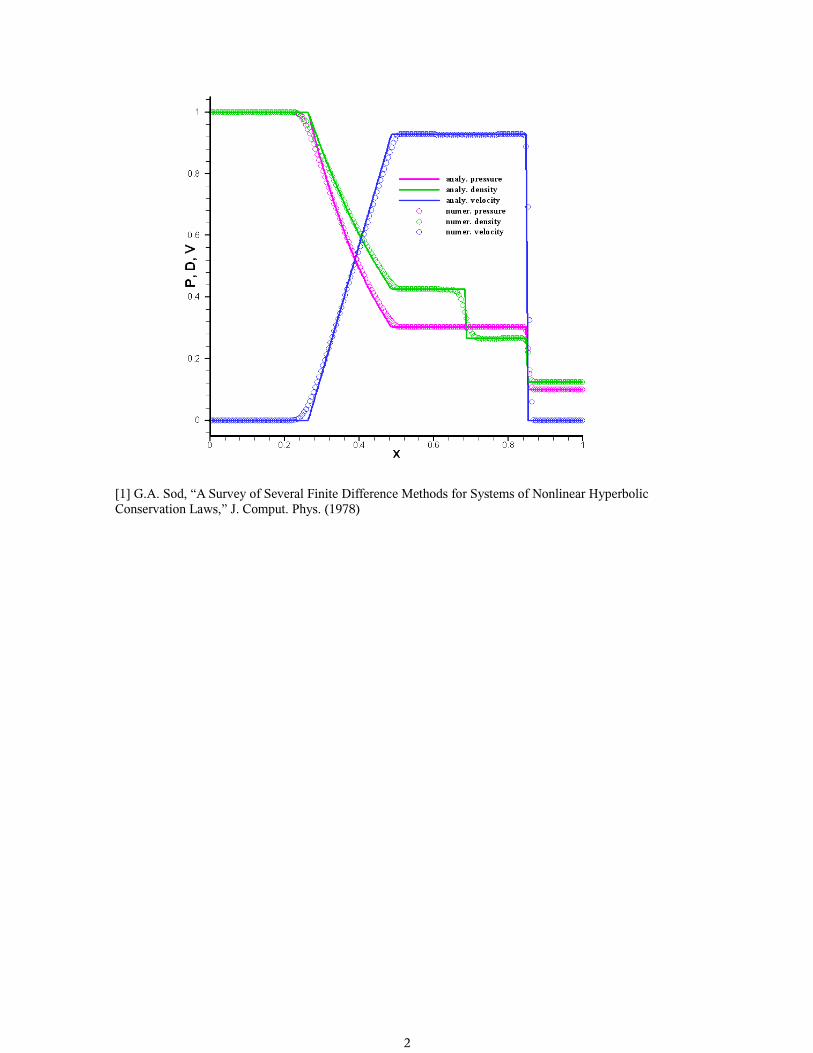
[1] G.A. Sod, “A Survey of Several Finite Difference Methods for Systems of Nonlinear Hyperbolic Conservation Laws,” J. Comput. Phys. (1978)

2

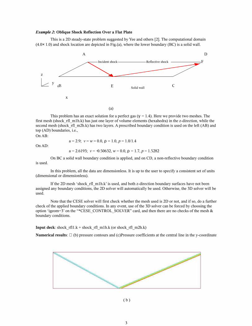
Example 2: Oblique Shock Reflection Over a Flat Plate

This is a 2D steady-state problem suggested by Yee and others [2]. The computational domain (4.0× 1.0) and shock location are depicted in Fig.(a), where the lower boundary (BC) is a solid wall.

(a)

This problem has an exact solution for a perfect gas (γ = 1.4). Here we provide two meshes. The first mesh (shock_rfl_m1h.k) has just one layer of volume elements (hexahedra) in the z-direction, while the second mesh (shock_rfl_m2h.k) has two layers. A prescribed boundary condition is used on the left (AB) and top (AD) boundaries, i.e.,On AB:

u = 2.9; v = w = 0.0, ρ = 1.0, p = 1.0/1.4On AD:

u = 2.6193; v = −0.50632, w = 0.0, ρ = 1.7, p = 1.5282

On BC a solid wall boundary condition is applied, and on CD, a non-reflective boundary condition is used.

In this problem, all the data are dimensionless. It is up to the user to specify a consistent set of units (dimensional or dimensionless).

If the 2D mesh ‘shock_rfl_m1h.k’ is used, and both z-direction boundary surfaces have not been assigned any boundary conditions, the 2D solver will automatically be used. Otherwise, the 3D solver will be used.

Note that the CESE solver will first check whether the mesh used is 2D or not, and if so, do a further check of the applied boundary conditions. In any event, use of the 3D solver can be forced by choosing the option ‘igeom=3’ on the “*CESE_CONTROL_SOLVER” card, and then there are no checks of the mesh & boundary conditions.

Input deck: shock_rfl1.k + shock_rfl_m1h.k (or shock_rfl_m2h.k)

Numerical results: (b) pressure contours and (c)Pressure coefficients at the central line in the y-coordinate

( b )

Solid wall

Reflective shockIncident shock

A D

F

CEB

x

z

y

3

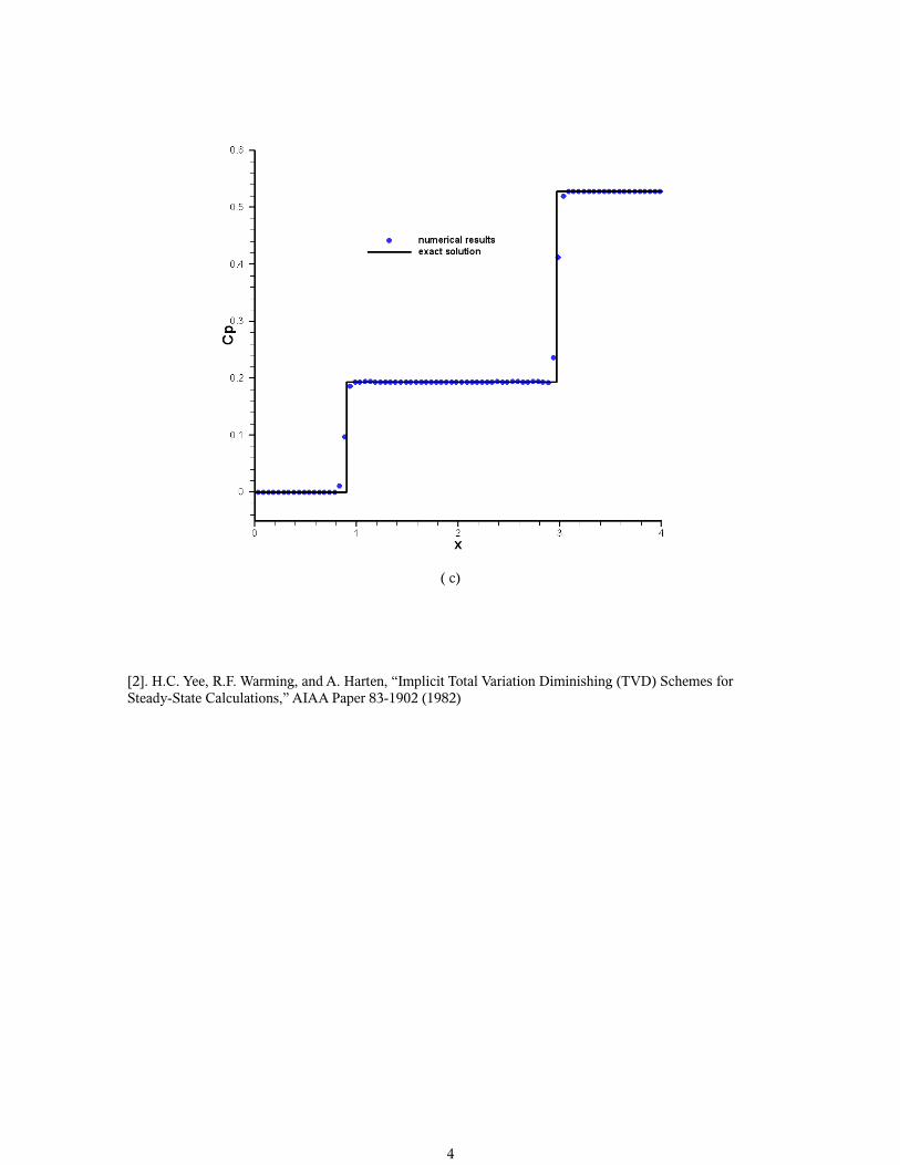
( c)

[2]. H.C. Yee, R.F. Warming, and A. Harten, “Implicit Total Variation Diminishing (TVD) Schemes for Steady-State Calculations,” AIAA Paper 83-1902 (1982)

4

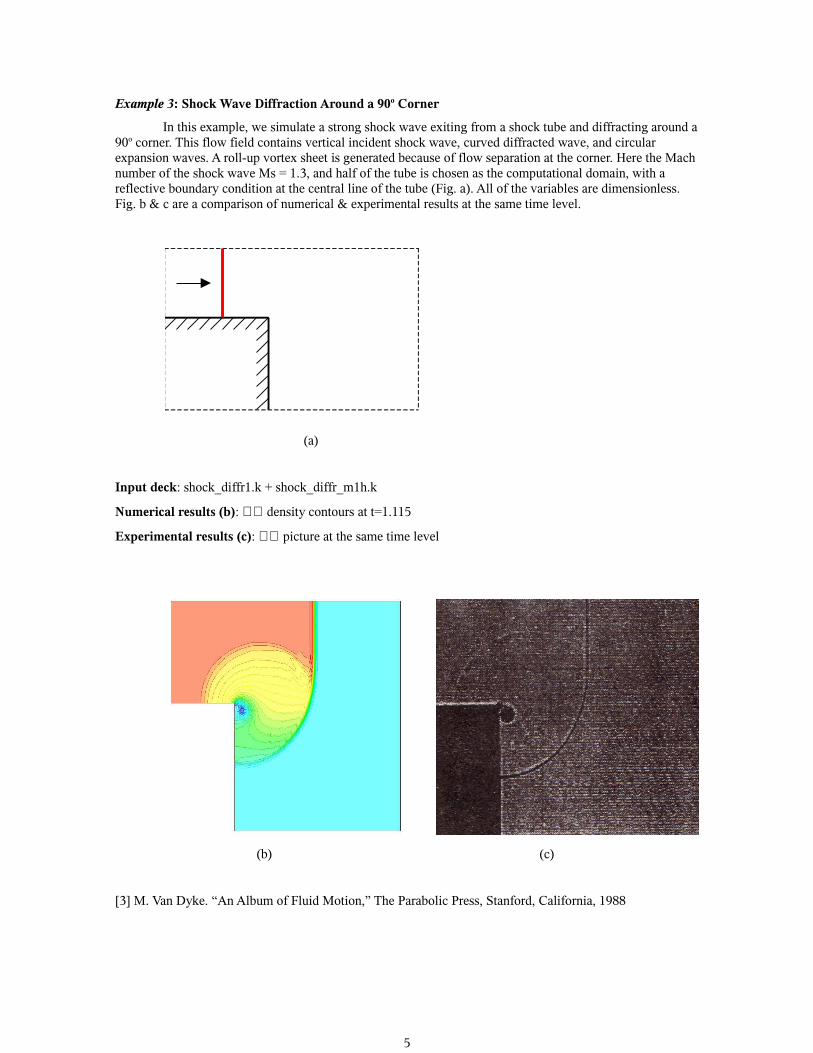
Example 3: Shock Wave Diffraction Around a 90o Corner

In this example, we simulate a strong shock wave exiting from a shock tube and diffracting around a 90o corner. This flow field contains vertical incident shock wave, curved diffracted wave, and circular expansion waves. A roll-up vortex sheet is generated because of flow separation at the corner. Here the Mach number of the shock wave Ms = 1.3, and half of the tube is chosen as the computational domain, with a reflective boundary condition at the central line of the tube (Fig. a). All of the variables are dimensionless. Fig. b & c are a comparison of numerical & experimental results at the same time level.

(a)

Input deck: shock_diffr1.k + shock_diffr_m1h.k

Numerical results (b): density contours at t=1.115

Experimental results (c): picture at the same time level

(b) (c)

[3] M. Van Dyke. “An Album of Fluid Motion,” The Parabolic Press, Stanford, California, 1988

5

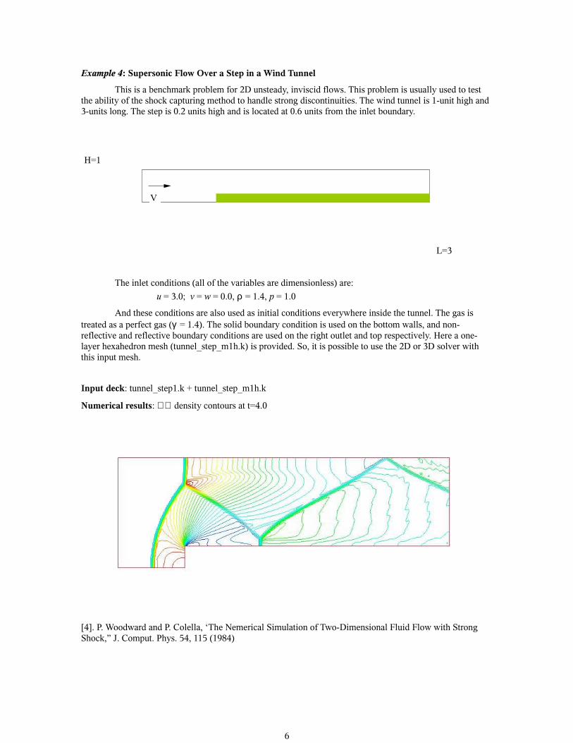
Example 4: Supersonic Flow Over a Step in a Wind Tunnel

This is a benchmark problem for 2D unsteady, inviscid flows. This problem is usually used to test the ability of the shock capturing method to handle strong discontinuities. The wind tunnel is 1-unit high and 3-units long. The step is 0.2 units high and is located at 0.6 units from the inlet boundary.

The inlet conditions (all of the variables are dimensionless) are:

u = 3.0; v = w = 0.0, ρ = 1.4, p = 1.0

And these conditions are also used as initial conditions everywhere inside the tunnel. The gas is treated as a perfect gas (γ = 1.4). The solid boundary condition is used on the bottom walls, and non-reflective and reflective boundary conditions are used on the right outlet and top respectively. Here a one-layer hexahedron mesh (tunnel_step_m1h.k) is provided. So, it is possible to use the 2D or 3D solver with this input mesh.

Input deck: tunnel_step1.k + tunnel_step_m1h.k

Numerical results: density contours at t=4.0

[4]. P. Woodward and P. Colella, ‘The Nemerical Simulation of Two-Dimensional Fluid Flow with Strong Shock,” J. Comput. Phys. 54, 115 (1984)

6

H=1

L=3

V

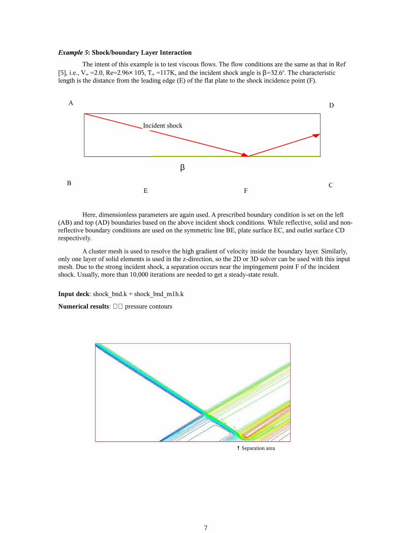
Example 5: Shock/boundary Layer Interaction

The intent of this example is to test viscous flows. The flow conditions are the same as that in Ref [5], i.e., V∞ =2.0, Re=2.96× 105, T∞ =117K, and the incident shock angle is β=32.6o. The characteristic length is the distance from the leading edge (E) of the flat plate to the shock incidence point (F).

Here, dimensionless parameters are again used. A prescribed boundary condition is set on the left (AB) and top (AD) boundaries based on the above incident shock conditions. While reflective, solid and non-reflective boundary conditions are used on the symmetric line BE, plate surface EC, and outlet surface CD respectively.

A cluster mesh is used to resolve the high gradient of velocity inside the boundary layer. Similarly, only one layer of solid elements is used in the z-direction, so the 2D or 3D solver can be used with this input mesh. Due to the strong incident shock, a separation occurs near the impingement point F of the incident shock. Usually, more than 10,000 iterations are needed to get a steady-state result.

Input deck: shock_bnd.k + shock_bnd_m1h.k

Numerical results: pressure contours

7

β

Incident shock

FE

D

B C

A

↑ Separation area

[5]. Hakkinen, R.J., Greber, I., Trilling, L. and Abarbanel, S.S., “The Interaction of an Oblique Shock Wave with a Laminar Boundary Layer,” NASA Memo 2-18-59W, 1959.

8

0 0.5 1 1.5x

­1

0

1

2

3

4

CfX

1000

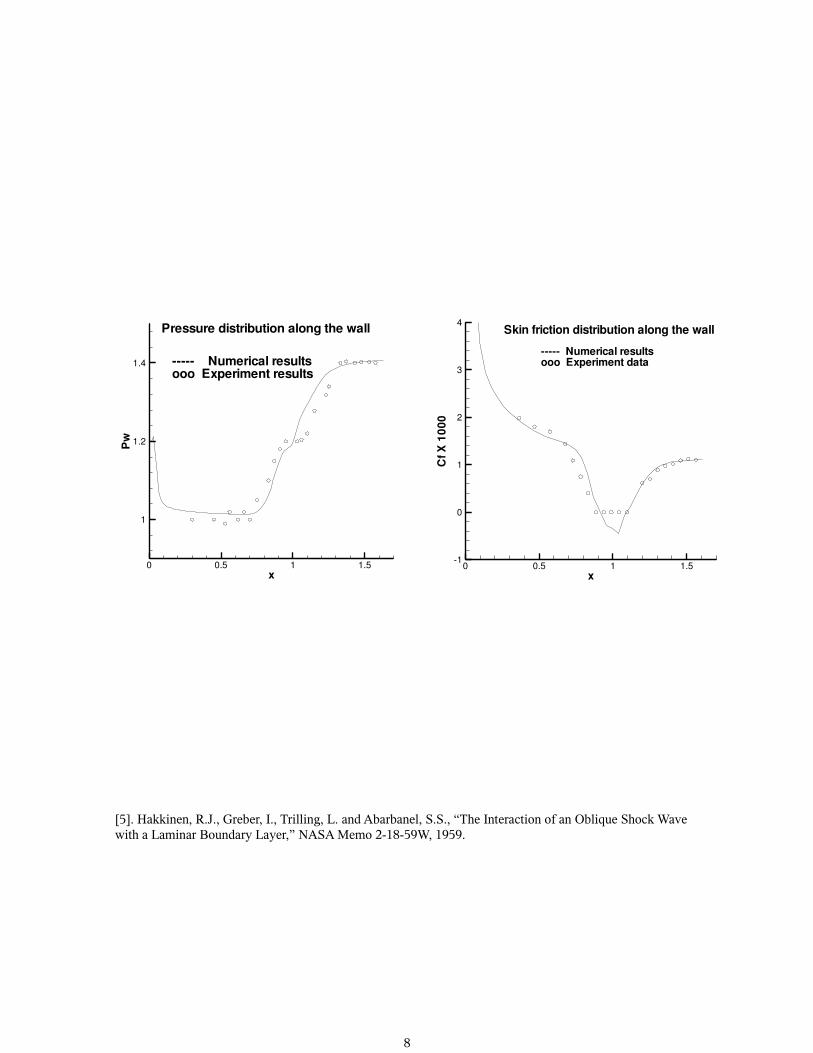
Skin friction distribution along the wall

­­­­­ Numerical resultsooo Experiment data

0 0.5 1 1.5x

1

1.2

1.4

Pw

Pressure distribution along the wall

­­­­­ Numerical resultsooo Experiment results

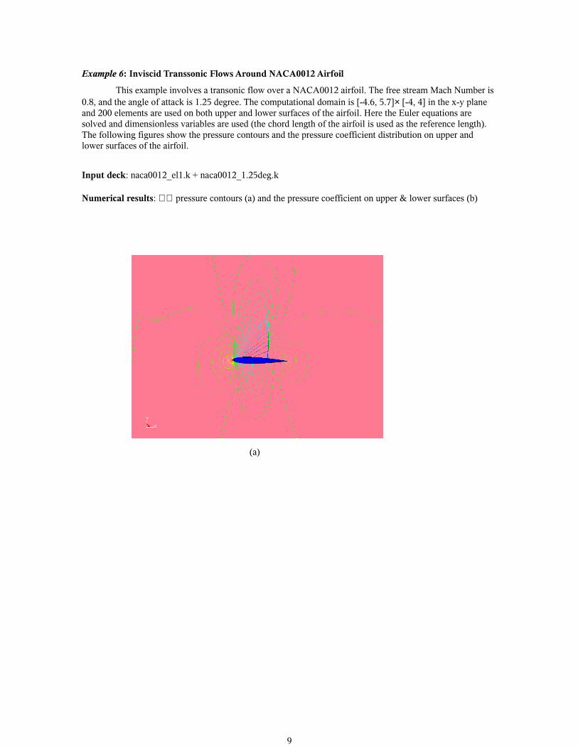
Example 6: Inviscid Transsonic Flows Around NACA0012 Airfoil

This example involves a transonic flow over a NACA0012 airfoil. The free stream Mach Number is 0.8, and the angle of attack is 1.25 degree. The computational domain is [-4.6, 5.7]× [-4, 4] in the x-y plane and 200 elements are used on both upper and lower surfaces of the airfoil. Here the Euler equations are solved and dimensionless variables are used (the chord length of the airfoil is used as the reference length). The following figures show the pressure contours and the pressure coefficient distribution on upper and lower surfaces of the airfoil.

Input deck: naca0012_el1.k + naca0012_1.25deg.k

Numerical results: pressure contours (a) and the pressure coefficient on upper & lower surfaces (b)

(a)

9

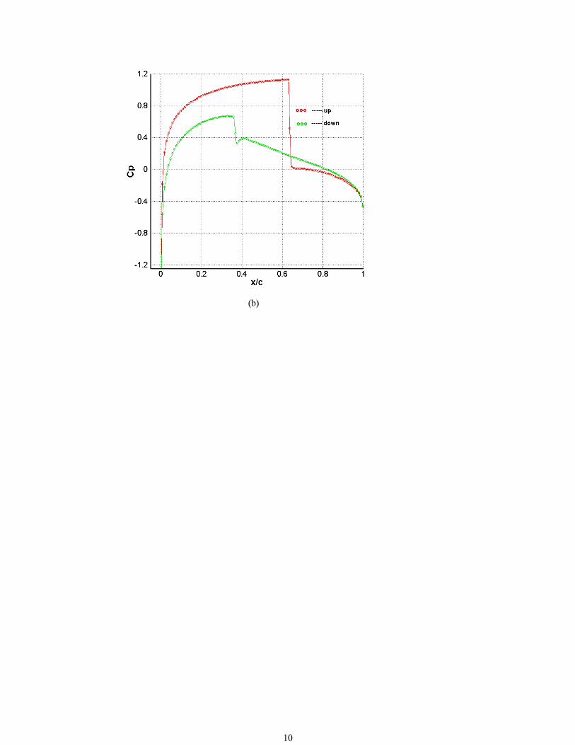
(b)

10

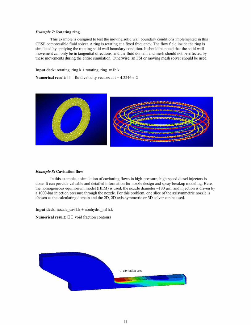
Example 7: Rotating ring

This example is designed to test the moving solid wall boundary conditions implemented in this CESE compressible fluid solver. A ring is rotating at a fixed frequency. The flow field inside the ring is simulated by applying the rotating solid wall boundary condition. It should be noted that the solid wall movement can only be in tangential directions, and the fluid domain and mesh should not be affected by these movements during the entire simulation. Otherwise, an FSI or moving mesh solver should be used.

Input deck: rotating_ring.k + rotating_ring_m1h.k

Numerical result: fluid velocity vectors at t = 4.2246 e-2

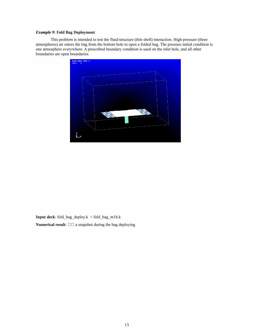
Example 8: Cavitation flow

In this example, a simulation of cavitating flows in high-pressure, high-speed diesel injectors is done. It can provide valuable and detailed information for nozzle design and spray breakup modeling. Here, the homogeneous equilibrium model (HEM) is used, the nozzle diameter =180 µm, and injection is driven by a 1000-bar injection pressure through the nozzle. For this problem, one slice of the axisymmetric nozzle is chosen as the calculating domain and the 2D, 2D axis-symmetric or 3D solver can be used.

Input deck: nozzle_cav1.k + nonhydro_m1h.k

Numerical result: void fraction contours

11

↓ cavitation area

12

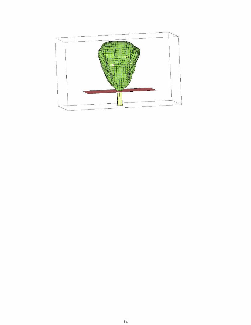
Example 9: Fold Bag Deployment

This problem is intended to test the fluid/structure (thin shell) interaction. High-pressure (three atmospheres) air enters the bag from the bottom hole to open a folded bag. The pressure initial condition is one atmosphere everywhere. A prescribed boundary condition is used on the inlet hole, and all other boundaries are open boundaries.

Input deck: fold_bag_deploy.k + fold_bag_m1h.k

Numerical result: a snapshot during the bag deploying

13

14

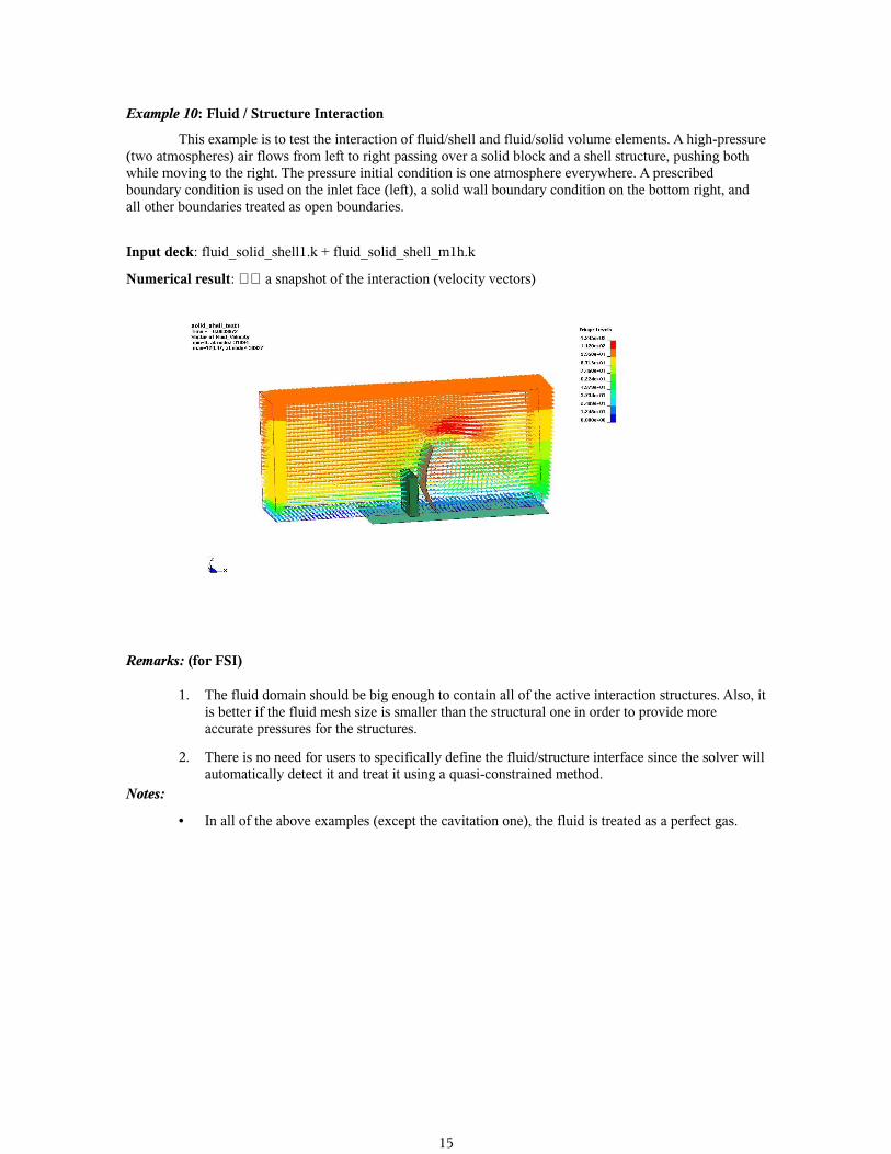
Example 10: Fluid / Structure Interaction

This example is to test the interaction of fluid/shell and fluid/solid volume elements. A high-pressure (two atmospheres) air flows from left to right passing over a solid block and a shell structure, pushing both while moving to the right. The pressure initial condition is one atmosphere everywhere. A prescribed boundary condition is used on the inlet face (left), a solid wall boundary condition on the bottom right, and all other boundaries treated as open boundaries.

Input deck: fluid_solid_shell1.k + fluid_solid_shell_m1h.k

Numerical result: a snapshot of the interaction (velocity vectors)

Remarks: (for FSI)

1. The fluid domain should be big enough to contain all of the active interaction structures. Also, it is better if the fluid mesh size is smaller than the structural one in order to provide more accurate pressures for the structures.

2. There is no need for users to specifically define the fluid/structure interface since the solver will automatically detect it and treat it using a quasi-constrained method.

Notes:

• In all of the above examples (except the cavitation one), the fluid is treated as a perfect gas.

15