Journal of Wind Engineering & Industrial Aerodynamics 177 (2018) 293–305

Contents lists available at ScienceDirect

Journal of Wind Engineering & Industrial Aerodynamics

journal homepage: www.elsevier.com/locate/jweia

Numerical study of turbulent flow fields around of a row of trees and anisolated building by using modified k-ε model and LES model

Yihong Qi *, Takeshi Ishihara

Department of Civil Engineering, School of Engineering, The University of Tokyo, Tokyo, Japan

A R T I C L E I N F O

Keywords:Turbulent flow fields over urban elementsModified k�ε modelLES modelValidation metricsVortex coresQuadrant analysis

* Corresponding author.E-mail address: qi@bridge.t.u-tokyo.ac.jp (Y. Qi)

https://doi.org/10.1016/j.jweia.2018.04.007Received 12 July 2017; Received in revised form 1

0167-6105/© 2018 Elsevier Ltd. All rights reserved

A B S T R A C T

Turbulent flow fields over two typical urban elements, a row of trees with low packing density and an isolatedbuilding with high packing density, are investigated by a modified k� ε model and a LES model. The applicabilityof these two models is evaluated by the validation metrics. Instantaneous flow fields are visualized by vortex coresand examined by quadrant analysis. In the wake region of the row of trees, predicted mean wind speed by themodified k� ε model shows favourable agreement with the measured data, but turbulent kinetic energy isunderestimated since the modified k� εmodel is not capable of simulating organized motions. In the wake regionof the isolated building, both predicted mean wind speed and turbulent kinetic energy by the modified k� εmodel are slightly underestimated due to lack of the vortex shedding in the simulation. On the other hand, LESmodel well predicts both mean wind speed and turbulent kinetic energy since all large vortices are directlyresolved by LES model.

1. Introduction

With increasing requirement on renewable energy, wind turbines areinstalled in or near the urban and suburban areas, where the local windcondition is strongly affected by surrounding trees and buildings. Pre-diction of mean wind speed and turbulence are important, because meanwind speed is directly related to potential wind energy, while turbulenceresults in fluctuating wind load on the structure components and affectsthe fatigue life of wind turbine. Therefore, accurate prediction of tur-bulent flow fields around trees and buildings is necessary not only fordesigning of wind turbine but also for maintenance of wind turbines (IEC61400-2, 2006).

With the aim of providing accurate prediction of turbulent flow fieldin the urban area, modelling of the effect of surface roughness is a keyfactor. Surface roughness trees and buildings are dominant and model-ling them is necessary. As to modelling buildings, the rigid wall approachwas applied by many researches (Gousseau et al. (2011), Blocken et al.(2012), Philips et al. (2013) and Cheng and Porte-Agel (Cheng andPort�e-Agel, 2015), Mochida et al. (2002), Tominaga et al. (2008) andGousseau et al. (2013)), in which detailed geometry information of eachbuilding are used and wall functions are applied for the boundary con-dition of building surface. However, this approach requires large efforton grid generation and calculation, and its application is therefore

.

October 2017; Accepted 9 April

.

limited to a small area. On modelling vegetation, the canopy model is theonly choice, which considers the fluid force and, turbulence generationand dissipation due to obstacles by introducing source terms into themomentum equation and turbulence transportation equations. Re-searches on canopy model with Reynolds average turbulence model(RANS) for vegetation and unban canopies have been carried out byWilson (1988), Green (1992), Liu et al. (1996), Aumond et al. (2013),Suzuki et al. (2002) and Iwata et al. (2004), Maruyama (1993), Salimet al. (2015). However, conventional canopy models have a limitationthat they can only be applicable to the canopy with a low packing den-sity. Moreover, Mochida et al. (2008) provided a detailed comparison ofvarious RANSmodels for the simulation of the wind flow through the rowof trees, but the organized motions around them and the reason of dis-crepancies between predicted and measured turbulent flow fields shouldbe further demonstrated. Enoki et al. (2009) and Enoki and Ishihara(2012) proposed a generalized canopy model which is able to considerthe effect of the vegetation and buildings simultaneously. The general-ized canopy model together with a modified k� ε model has beenapplied for wind prediction of a single building as well as a real urbanarea. Comparing with rigid wall approach, the canopy model relax therequirement of geometry in the region close to obstacles, and it allowsless computational grid. Furthermore, a simple grid system can be used inany size of urban areas. However, there are still some discrepancies

2018

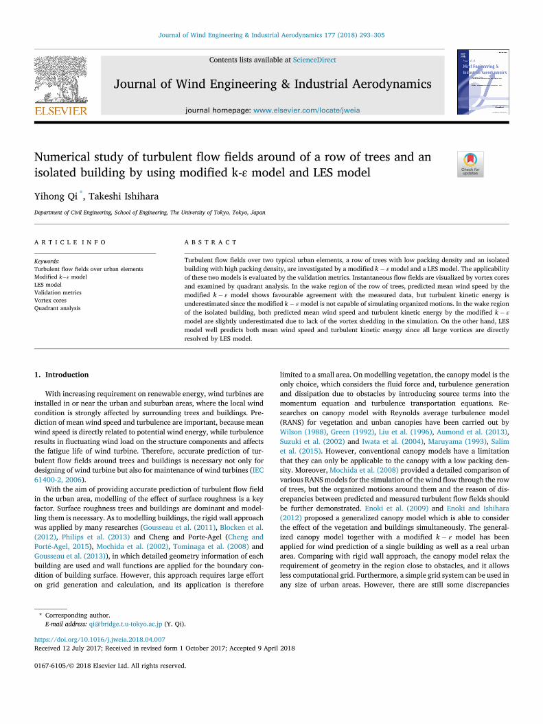
Table 1Parameters in the conventional and the generalized canopy models.

Type of obstacles Conventionalcanopy model

Generalized canopy model

Vegetation (Wilson,1988)

fu;i ¼ �12ρCD;t at jujui

Cf ¼ CD;t

γ0 ¼ at l0l0 ¼ 10�3ðmÞ

Buildings(Maruyama,1993)

fu;i ¼ �12ρCD;bab jujui

Cf ¼ CD;b=ð1� γbÞ3 ¼

1ð1� γbÞ3

min�1:531� γb

;2:75ð1� γbÞ�

γb ¼ Vb=Vgrid γ0 ¼ γb

ab ¼ Sb4ð1� γbÞVgrid

l0 ¼ 4Vb=Sb ðmÞ

Y. Qi, T. Ishihara Journal of Wind Engineering & Industrial Aerodynamics 177 (2018) 293–305

between predicted and measured flow field and the reasons should beinvestigated. Moreover, accuracy of the LES model with the generalizedcanopy model has not been evaluated yet.

LES models are also used with rigid wall approach to predict unsteadyflow fields over buildings (Rodi (1997), Yoshie et al., 2007, 2011 and Xieand Castro (2006)). They attributed the good performance of LES modelto predict periodic vortex shedding and highlighted the importance ofinflow turbulence on the accuracy of simulation using LES model. Onmodelling trees, some efforts were also made by using LES model (Yanget al. (2006), Bailey and Stoll (2013), Mueller et al. (2014) and Lopeset al. (2013)). However, accurate prediction with LES model depends onseveral issues, such as turbulent inflow condition and grid resolution.Therefore, a comparison between RANS and LES models for canopy flowswith low and high packing densities is necessary to clarify the applica-bility of each turbulence model.

In this study, the numerical methods are given in section 2, includinggoverning equations, fluid force and turbulence models, boundary con-dition and numerical schemes used in the simulations, as well as analysismethods applied in the discussion. In section 3, two typical urban ele-ments are discussed. At first, the experiment in each case is brieflydescribed, then turbulent flow fields are investigated and applicability ofthese two models is evaluated by the validation metrics. Instantaneousflow fields are visualized by vortex cores and examined by the quadrantanalysis. Finally, conclusions are shown in section 4 based on abovediscussions.

2. Numerical method

2.1. Governing equations

For the analysis of the flow field with obstacles inside, two differentapproaches are used. The governing equations are constructed for thefluid part only in one approach, and for the flow field averaged over thecomputational grid in the other approach. In this study, the latterapproach is used. The averaged continuity and momentum equations forincompressible flow with considering the effect of the buildings andvegetation are given by:

∂ðρuiÞ∂xi

¼ 0 (1)

∂ðρuiÞ∂t þ ∂

�ρujui

�∂xj

¼ �∂p∂xi

þ ∂∂xj

�μ�∂ui∂xj

þ ∂uj∂xi

��þ ∂τij

∂xjþ fu;i (2)

where ui is the wind velocity in the ith direction (u1 ¼ u; u2 ¼ v and u3 ¼w). p is pressure, ρ is density of the fluid, μ is the molecular viscosity andfu;i is the fluid force per unit grid volume due to obstacles which isdescribed in section 2.2. The overbar indicates time averagedmean valuein the simulation with the modified k� ε model, while it indicates theresolved value in the simulation with LES model. τij is introduced toconsider difference between uiuj and uiuj, i.e.,

τij ¼ �ρ�uiuj � uiuj

(3)

Although the expression of τij in Eq. (3) is the same for the modifiedk� ε model and the LES model, its meaning is different in the twomodels. τij in the modified k� ε model is time-averaged Reynolds stressand stands for effect from vortex to mean flow field, while τij in LES in-dicates the subgrid-scale Reynolds stress and accounts for contributionfrom unresolved smaller vortex to large size vortex.

2.2. Fuid force model

The generalized canopy model derived by Enoki and Ishihara (2012)is applied in this study and the fluid force in the momentum equations is:

294

fu;i ¼ � Fu;i

Vgrid¼ �1

2ρCf

γ0l0jujui (4)

where, fu;i is the fluid force in the volume of grid, Vgrid. juj is the absolutevalue of mean wind speed per unit volume, Cf is the equivalent dragcoefficient, l0 is defined as the representative length scale of obstaclesand γ0 is the packing density. Canopy parameters for vegetation andbuildings are summarized in Table 1, where CD;t and at are the dragcoefficient and the leaf area density of vegetation respectively, CD;b, Vb

and Sb are the drag coefficient, the total volume and the total side surfaceof buildings.

2.3. Turbulence model

For the closure of the governing equations, τij has to be modelled. Inthe modified k� ε model, τij is approximated by the linear turbulenceviscosity model, i.e.,

τij ¼ �ρu0iu

0j ¼ 2μtSij �

23ρkδij (5)

where δij is the Kronecker delta. Turbulence viscosity μt and rate-of-straintensor Sij are expressed as:

μt ¼ Cμρk2

ε(6)

Sij ¼ 12

�∂ui∂xj

þ ∂uj∂xi

�(7)

In the modified k� ε model, two additional equations are used tocalculate the turbulent kinetic energy, k, and the dissipation rate, ε.

∂ρk∂t þ ∂ρujk

∂xj¼ ∂

∂xj

��μþ μt

σk

�∂k∂xj

���23ρkδij

∂ui∂xj

� Pk

�� ρεþ fk (8)

∂ρε∂t þ ∂ρujε

∂xj¼ ∂

∂xj

��μþ μt

σε

�∂ε∂xj

�� Cε1

ε

k

�23ρkδij

∂ui∂xj

� Pk

�� Cε2

ρε2

kþ fε

(9)

Parameters in the above equations are the same as those used in thestandard k� εmodel, i.e., Cμ ¼ 0:09, σk ¼ 1:0, Cε ¼ 1:3, Cε1 ¼ 1:44 andCε2 ¼ 1:92. In order to settle overestimation of turbulent kinetic energyat stagnation point, turbulence source term Pk is estimated by Kato andLaunder model (Kato, 1993). The source terms for turbulent kinetic en-ergy and its dissipation rate are introduced to consider the promotingprocess of energy cascade in canopy layer. The model proposed by Enokiand Ishihara (Enoki et al., 2009; Enoki and Ishihara, 2012) is adoptedand can be expressed as:

fk ¼ 12βpρCf a

u3 � 12βdρCf a

uk (10)

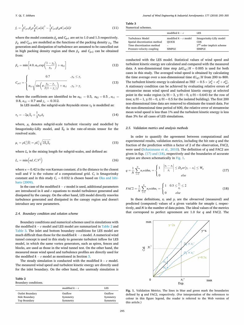
Table 3Numerical schemes.

modified k� ε LES

Turbulence Model modified k� ε model Smagorinsky-Lilly modelSpatial discretization method QUICK CDSTime discretization method – 2nd order implicit schemePressure-velocity coupling SIMPLE SIMPLE

Y. Qi, T. Ishihara Journal of Wind Engineering & Industrial Aerodynamics 177 (2018) 293–305

fε ¼ 12Cpε1βpρ

ε

kCf a

u3 � 12Cpε2βdρCf a

uε (11)

where the model constants βp and Cpε1 are set to 1.0 and 1.5 respectively.βd and Cpε2 are modelled as the functions of the packing density γ0. Thegeneration and dissipation of turbulence are assumed to be cancelled outin high packing density region and then βd and Cpε2 can be obtainedfrom:

βd ¼ min�4:0; αk1exp

�1� γ0γ0

�þ αk2

�(12)

Cpε2 ¼

8>><>>:

0:7 ; γ0 � γc

αε1

ffiffiffiffiffiffiffiffiffiffiffiffiffiffiffiffiffiffiffiffiffiffiffiffiffiffiffiffiffiffiffiffiffiffiffiffiffiffiffiffiffiffiffiffiffiffisin

�π

γ0 � γc2ð1� γcÞ

�þ αε2

s; γ0 > γc

(13)

where the coefficients are identified to be αk1 ¼ 0:5, αk2 ¼ 0:5 , αε1 ¼0:8, αε2 ¼ 0:7 and γc ¼ 0:312.

In LES model, the subgrid-scale Reynolds stress τij is modelled as:

τij ¼ �2μtSij þ13τkkδij (14)

where, μt denotes subgrid-scale turbulent viscosity and modelled bySmagorinsky-Lilly model, and Sij is the rate-of-strain tensor for theresolved scale.

μt ¼ ρL2s jSj ¼ ρL2

s

ffiffiffiffiffiffiffiffiffiffiffiffi2SijSij

q(15)

where Ls is the mixing length for subgrid-scales, and defined as:

Ls ¼ min�κd;CsV

13

(16)

where κ¼ 0.42 is the von Karman constant. d is the distance to the closestwall and V is the volume of a computational grid. Cs is Smagorinskyconstant and in this study Cs ¼ 0:032 is chosen based on Oka and Ishi-hara (2009).

In the case of the modified k� εmodel is used, additional parametersare introduced in k and ε equations to model turbulence generated anddissipated by the canopy. On the other hand, LES model directly resovlesturbulence generated and dissipated in the canopy region and doesn'tintroduce any new parameters.

2.4. Boundary condition and solution scheme

Boundary conditions and numerical schemes used in simulations withthe modified k� ε model and LES model are summarized in Table 2 andTable 3. The inlet and bottom boundary conditions for LES model aremuch difficult than those for the modified k� εmodel. A numerical windtunnel concept is used in this study to generate turbulent inflow for LESmodel, in which the same vortex generators, such as spires, fences andblocks, are used as those in the wind tunnel test. On the other hand, themeasured mean wind speed and turbulence profiles are directly used forthe modified k� ε model as mentioned in Section 3.

The steady simulation is conducted with the modified k� ε model.The measured wind speed and turbulent kinetic energy are directly usedfor the inlet boundary. On the other hand, the unsteady simulation is

Table 2Boundary conditions.

modified k� ε LES

Outlet Boundary Outflow OutflowSide Boundary Symmetry SymmetryTop Boundary Symmetry Symmetry

295

conducted with the LES model. Statistical values of wind speed andturbulent kinetic energy are calculated and compared with the measureddata. A non-dimensional time step ΔtUref =H ¼ 0:005 is used for bothcases in this study. The averaged wind speed is obtained by calculatingthe time average over a non-dimensional time tUref =H from 200 to 800.The turbulent kinetic energy is calculated as TKE ¼ 0:5� ½σ2u þ σ2v þ σ2w�.A stationary condition can be achieved by evaluating relative errors ofstreamwise mean wind speed and turbulent kinetic energy at selectedpoint in the wake region (x/H¼ 3, y/H¼ 0, z/H¼ 0.643 for the row oftree; x/H¼ 1, y/H¼ 0, z/H¼ 0.5 for the isolated building). The first 200non-dimensional time data are removed to eliminate the transit data. Forthe non-dimensional time period of 600, the relative error of streamwisemean wind speed is less than 1% and the turbulent kinetic energy is lessthan 3% for all cases of LES simulations.

2.5. Validation metrics and analysis methods

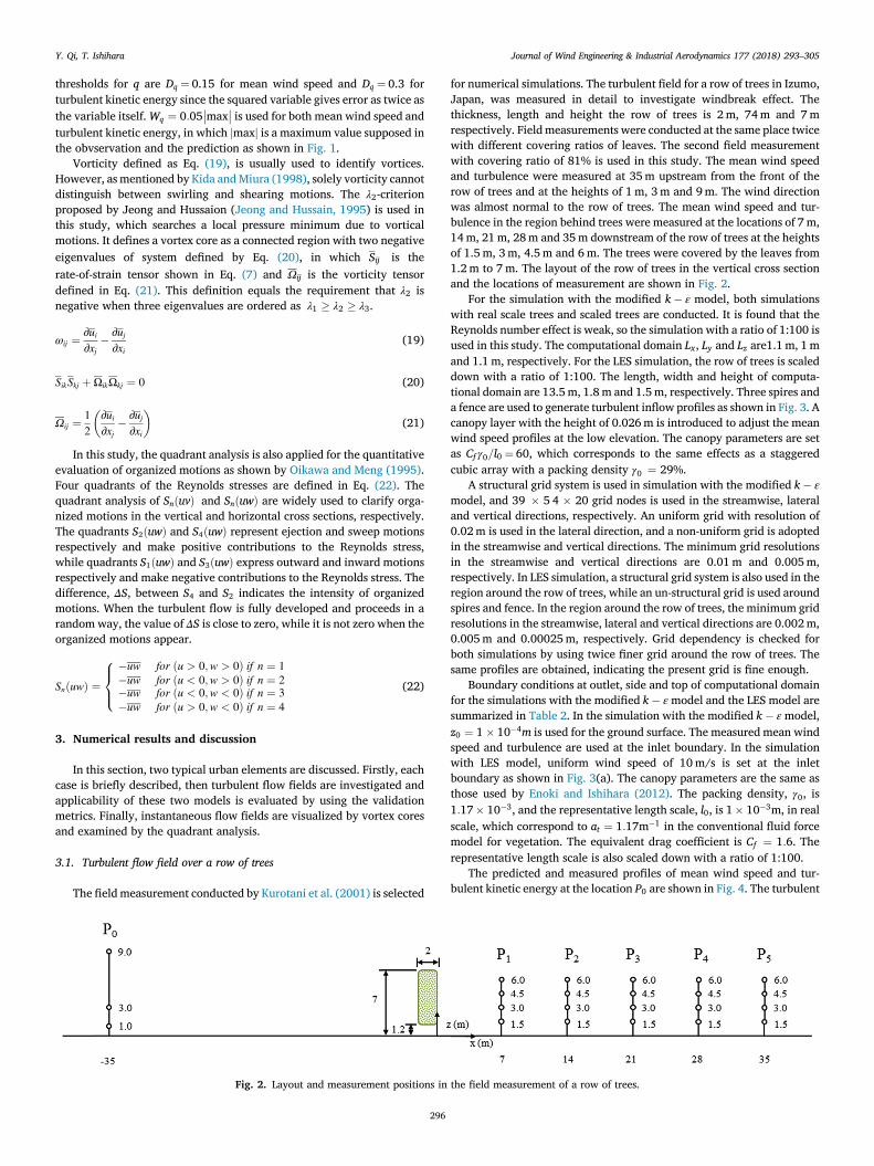
In order to quantify the agreement between computational andexperimental results, validation metrics, including the hit rate q and thefraction of the prediction within a factor of 2 of the observation, FAC2,were used (Schatzmann et al., 2010). The definition of q and FAC2 aregiven in Eqs. (17) and (18), respectively and the boundaries of accurateregion are shown schematically in Fig. 1.

q ¼ 1N

XNi¼1

niwithni ¼8<: 1

yi � xixi

� Dqoryi � xi

� Wq

0 else

(17)

FAC2 ¼ 1N

XNi¼1

niwithni ¼8<:

1 0:5 � yixi� 2

0 else(18)

In these definitions, xi and yi are the obvserved (measured) andpredicted (computed) values of a given variable for smaple i, respec-tively, and N is the number of data points. The ideal values of the metricsthat correspond to perfect agreement are 1.0 for q and FAC2. The

Fig. 1. Validation Metrics. The lines in blue and green mark the boundariesdefined by q and FAC2, respectively. (For interpretation of the references tocolour in this figure legend, the reader is referred to the Web version ofthis article.)

Y. Qi, T. Ishihara Journal of Wind Engineering & Industrial Aerodynamics 177 (2018) 293–305

thresholds for q are Dq ¼ 0.15 for mean wind speed and Dq ¼ 0.3 forturbulent kinetic energy since the squared variable gives error as twice asthe variable itself.Wq ¼ 0:05

max is used for both mean wind speed and

turbulent kinetic energy, in which jmaxj is a maximum value supposed inthe obvservation and the prediction as shown in Fig. 1.

Vorticity defined as Eq. (19), is usually used to identify vortices.However, as mentioned by Kida andMiura (1998), solely vorticity cannotdistinguish between swirling and shearing motions. The λ2-criterionproposed by Jeong and Hussaion (Jeong and Hussain, 1995) is used inthis study, which searches a local pressure minimum due to vorticalmotions. It defines a vortex core as a connected region with two negativeeigenvalues of system defined by Eq. (20), in which Sij is therate-of-strain tensor shown in Eq. (7) and Ωij is the vorticity tensordefined in Eq. (21). This definition equals the requirement that λ2 isnegative when three eigenvalues are ordered as λ1 � λ2 � λ3.

ωij ¼ ∂ui∂xj

� ∂uj∂xi

(19)

SikSkj þ ΩikΩkj ¼ 0 (20)

Ωij ¼ 12

�∂ui∂xj

� ∂uj∂xi

�(21)

In this study, the quadrant analysis is also applied for the quantitativeevaluation of organized motions as shown by Oikawa and Meng (1995).Four quadrants of the Reynolds stresses are defined in Eq. (22). Thequadrant analysis of SnðuvÞ and SnðuwÞ are widely used to clarify orga-nized motions in the vertical and horizontal cross sections, respectively.The quadrants S2ðuwÞ and S4ðuwÞ represent ejection and sweep motionsrespectively and make positive contributions to the Reynolds stress,while quadrants S1ðuwÞ and S3ðuwÞ express outward and inward motionsrespectively and make negative contributions to the Reynolds stress. Thedifference, ΔS, between S4 and S2 indicates the intensity of organizedmotions. When the turbulent flow is fully developed and proceeds in arandomway, the value of ΔS is close to zero, while it is not zero when theorganized motions appear.

SnðuwÞ ¼�uw�uw

for ðu > 0;w > 0Þ if n ¼ 1for ðu < 0;w > 0Þ if n ¼ 2

�uw�uw

for ðu < 0;w < 0Þ if n ¼ 3for ðu > 0;w < 0Þ if n ¼ 4

8><>: (22)

3. Numerical results and discussion

In this section, two typical urban elements are discussed. Firstly, eachcase is briefly described, then turbulent flow fields are investigated andapplicability of these two models is evaluated by using the validationmetrics. Finally, instantaneous flow fields are visualized by vortex coresand examined by the quadrant analysis.

3.1. Turbulent flow field over a row of trees

The field measurement conducted by Kurotani et al. (2001) is selected

Fig. 2. Layout and measurement positions in

296

for numerical simulations. The turbulent field for a row of trees in Izumo,Japan, was measured in detail to investigate windbreak effect. Thethickness, length and height the row of trees is 2 m, 74m and 7mrespectively. Fieldmeasurements were conducted at the same place twicewith different covering ratios of leaves. The second field measurementwith covering ratio of 81% is used in this study. The mean wind speedand turbulence were measured at 35m upstream from the front of therow of trees and at the heights of 1 m, 3m and 9m. The wind directionwas almost normal to the row of trees. The mean wind speed and tur-bulence in the region behind trees were measured at the locations of 7m,14m, 21m, 28m and 35m downstream of the row of trees at the heightsof 1.5 m, 3m, 4.5m and 6m. The trees were covered by the leaves from1.2m to 7m. The layout of the row of trees in the vertical cross sectionand the locations of measurement are shown in Fig. 2.

For the simulation with the modified k� ε model, both simulationswith real scale trees and scaled trees are conducted. It is found that theReynolds number effect is weak, so the simulation with a ratio of 1:100 isused in this study. The computational domain Lx, Ly and Lz are1.1m, 1mand 1.1m, respectively. For the LES simulation, the row of trees is scaleddown with a ratio of 1:100. The length, width and height of computa-tional domain are 13.5m, 1.8 m and 1.5m, respectively. Three spires anda fence are used to generate turbulent inflow profiles as shown in Fig. 3. Acanopy layer with the height of 0.026m is introduced to adjust the meanwind speed profiles at the low elevation. The canopy parameters are setas Cf γ0=l0 ¼ 60, which corresponds to the same effects as a staggeredcubic array with a packing density γ0 ¼ 29%.

A structural grid system is used in simulation with the modified k� εmodel, and 39 � 5 4 � 20 grid nodes is used in the streamwise, lateraland vertical directions, respectively. An uniform grid with resolution of0.02m is used in the lateral direction, and a non-uniform grid is adoptedin the streamwise and vertical directions. The minimum grid resolutionsin the streamwise and vertical directions are 0.01m and 0.005m,respectively. In LES simulation, a structural grid system is also used in theregion around the row of trees, while an un-structural grid is used aroundspires and fence. In the region around the row of trees, the minimum gridresolutions in the streamwise, lateral and vertical directions are 0.002m,0.005m and 0.00025m, respectively. Grid dependency is checked forboth simulations by using twice finer grid around the row of trees. Thesame profiles are obtained, indicating the present grid is fine enough.

Boundary conditions at outlet, side and top of computational domainfor the simulations with the modified k� εmodel and the LES model aresummarized in Table 2. In the simulation with the modified k� εmodel,z0 ¼ 1� 10�4m is used for the ground surface. The measured mean windspeed and turbulence are used at the inlet boundary. In the simulationwith LES model, uniform wind speed of 10m/s is set at the inletboundary as shown in Fig. 3(a). The canopy parameters are the same asthose used by Enoki and Ishihara (2012). The packing density, γ0, is1:17� 10�3, and the representative length scale, l0, is 1� 10�3m, in realscale, which correspond to at ¼ 1:17m�1 in the conventional fluid forcemodel for vegetation. The equivalent drag coefficient is Cf ¼ 1:6. Therepresentative length scale is also scaled down with a ratio of 1:100.

The predicted and measured profiles of mean wind speed and tur-bulent kinetic energy at the location P0 are shown in Fig. 4. The turbulent

the field measurement of a row of trees.

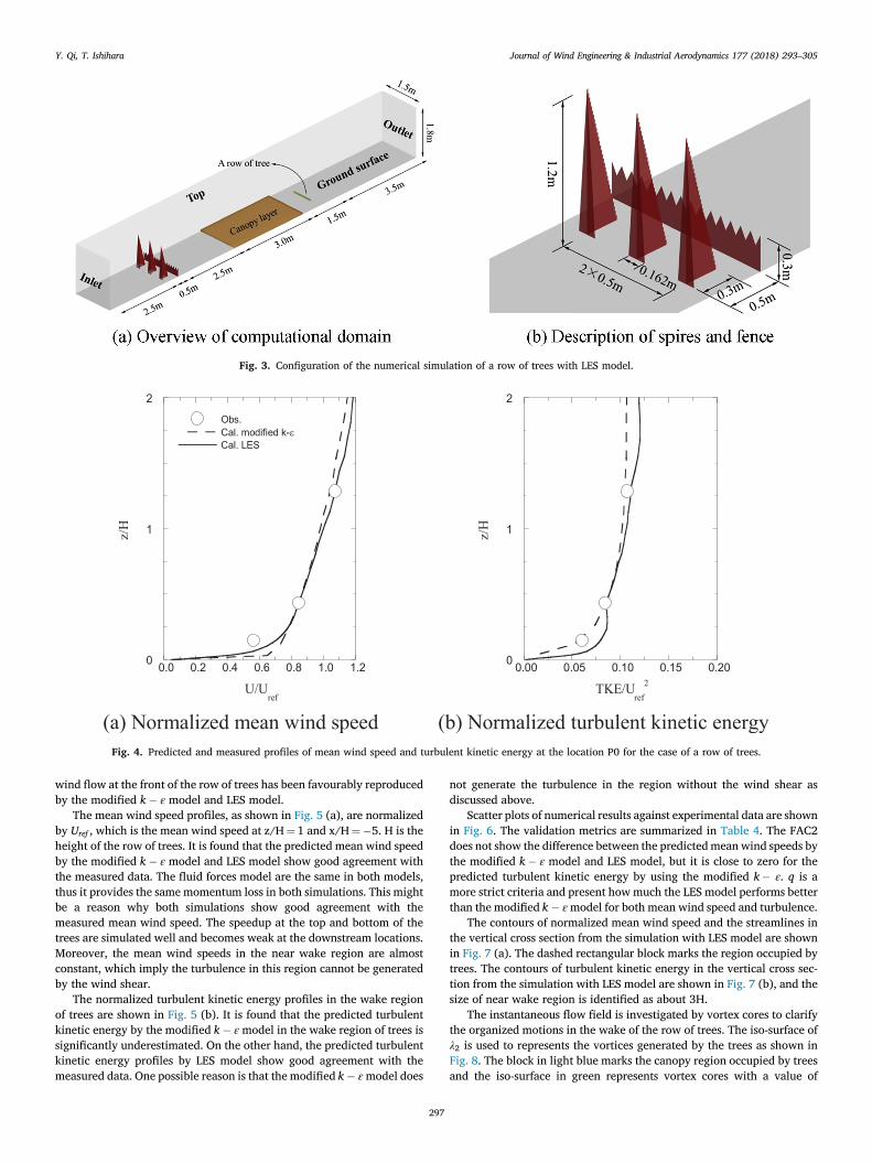
Fig. 3. Configuration of the numerical simulation of a row of trees with LES model.

Fig. 4. Predicted and measured profiles of mean wind speed and turbulent kinetic energy at the location P0 for the case of a row of trees.

Y. Qi, T. Ishihara Journal of Wind Engineering & Industrial Aerodynamics 177 (2018) 293–305

wind flow at the front of the row of trees has been favourably reproducedby the modified k� ε model and LES model.

The mean wind speed profiles, as shown in Fig. 5 (a), are normalizedby Uref , which is the mean wind speed at z/H¼ 1 and x/H¼�5. H is theheight of the row of trees. It is found that the predicted mean wind speedby the modified k� ε model and LES model show good agreement withthe measured data. The fluid forces model are the same in both models,thus it provides the same momentum loss in both simulations. This mightbe a reason why both simulations show good agreement with themeasured mean wind speed. The speedup at the top and bottom of thetrees are simulated well and becomes weak at the downstream locations.Moreover, the mean wind speeds in the near wake region are almostconstant, which imply the turbulence in this region cannot be generatedby the wind shear.

The normalized turbulent kinetic energy profiles in the wake regionof trees are shown in Fig. 5 (b). It is found that the predicted turbulentkinetic energy by the modified k� ε model in the wake region of trees issignificantly underestimated. On the other hand, the predicted turbulentkinetic energy profiles by LES model show good agreement with themeasured data. One possible reason is that the modified k� εmodel does

297

not generate the turbulence in the region without the wind shear asdiscussed above.

Scatter plots of numerical results against experimental data are shownin Fig. 6. The validation metrics are summarized in Table 4. The FAC2does not show the difference between the predictedmean wind speeds bythe modified k� ε model and LES model, but it is close to zero for thepredicted turbulent kinetic energy by using the modified k� ε. q is amore strict criteria and present how much the LES model performs betterthan the modified k� εmodel for both mean wind speed and turbulence.

The contours of normalized mean wind speed and the streamlines inthe vertical cross section from the simulation with LES model are shownin Fig. 7 (a). The dashed rectangular block marks the region occupied bytrees. The contours of turbulent kinetic energy in the vertical cross sec-tion from the simulation with LES model are shown in Fig. 7 (b), and thesize of near wake region is identified as about 3H.

The instantaneous flow field is investigated by vortex cores to clarifythe organized motions in the wake of the row of trees. The iso-surface ofλ2 is used to represents the vortices generated by the trees as shown inFig. 8. The block in light blue marks the canopy region occupied by treesand the iso-surface in green represents vortex cores with a value of

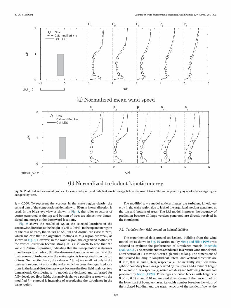
Fig. 5. Predicted and measured profiles of mean wind speed and turbulent kinetic energy behind the row of trees. The rectangular in gray marks the canopy regionoccupied by trees.

Y. Qi, T. Ishihara Journal of Wind Engineering & Industrial Aerodynamics 177 (2018) 293–305

λ2 ¼ -2000. To represent the vortices in the wake region clearly, thecentral part of the computational domain with 50m in lateral direction isused. In the bird's eye view as shown in Fig. 8, the roller structures ofvortex generated at the top and bottom of trees are almost two dimen-sional and merge at the downward locations.

Fig. 9 shows the results of ΔS at the selected locations in thestreamwise direction at the height of z/H¼ 0.643. In the upstream regionof the row of trees, the values of ΔSðuwÞ and ΔSðuvÞ are close to zero,which indicate that the organized motions in this region are weak, asshown in Fig. 8. However, in the wake region, the organized motions inthe vertical direction become strong. It is also worth to note that thevalue of ΔSðuwÞ is positive, indicating that the sweep motion is strongerthan the ejection motion, thus the downwardmotion is dominant and themain source of turbulence in the wake region is transported from the topof tress. On the other hand, the values of ΔSðuvÞ are small not only in theupstream region but also in the wake, which express the organized mo-tions in the lateral direction are weak because the flow field is almost twodimensional. Considering k� ε models are designed and calibrated forfully developed flow fields, this analysis shows a possible reason why themodified k� ε model is incapable of reproducing the turbulence in thewake region.

298

The modified k� ε model underestimates the turbulent kinetic en-ergy in the wake region due to lack of the organized motions generated atthe top and bottom of trees. The LES model improves the accuracy ofprediction because all large vortices generated are directly resolved inthe simulation.

3.2. Turbulent flow field around an isolated building

The experimental data around an isolated building from the windtunnel test as shown in Fig. 10 carried out by Meng and Hibi (1998) wasselected to evaluate the performance of turbulence models (Mochidaet al., 2002). The experiment was conducted in a return wind tunnel witha test section of 1.1m wide, 0.9 m high and 7m long. The dimensions ofthe isolated building in longitudinal, lateral and vertical directions are0.08m, 0.08m and 0.16m, respectively. The neutrally stratified atmo-spheric boundary layer was generated by five spires and a fence of height0.6 m and 0.1m respectively, which are designed following the methodproposed by Irwin (1979). Three types of cubic blocks with heights of0.06m, 0.02m and 0.01m, are used downstream of the fence to adjustthe lower part of boundary layer. Reynolds number based on the width ofthe isolated building and the mean velocity of the incident flow at the

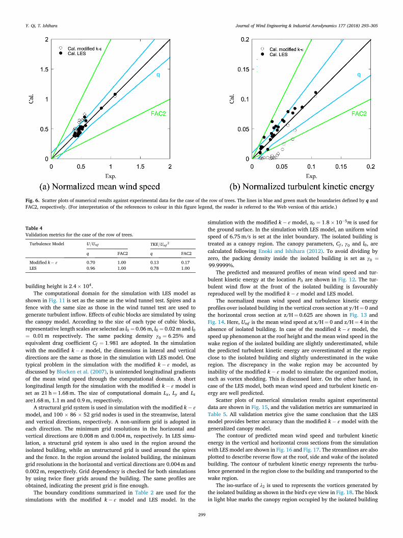
Fig. 6. Scatter plots of numerical results against experimental data for the case of the row of trees. The lines in blue and green mark the boundaries defined by q andFAC2, respectively. (For interpretation of the references to colour in this figure legend, the reader is referred to the Web version of this article.)

Table 4Validation metrics for the case of the row of trees.

Turbulence Model U=Uref TKE=Uref2

q FAC2 q FAC2

Modified k� ε 0.70 1.00 0.13 0.17LES 0.96 1.00 0.78 1.00

Y. Qi, T. Ishihara Journal of Wind Engineering & Industrial Aerodynamics 177 (2018) 293–305

building height is 2:4� 104.The computational domain for the simulation with LES model as

shown in Fig. 11 is set as the same as the wind tunnel test. Spires and afence with the same size as those in the wind tunnel test are used togenerate turbulent inflow. Effects of cubic blocks are simulated by usingthe canopy model. According to the size of each type of cubic blocks,representative length scales are selected as l0 ¼ 0.06m, l0 ¼ 0.02m and l0¼ 0.01m respectively. The same packing density γ0 ¼ 6:25% andequivalent drag coefficient Cf ¼ 1:981 are adopted. In the simulationwith the modified k� ε model, the dimensions in lateral and verticaldirections are the same as those in the simulation with LES model. Onetypical problem in the simulation with the modified k� ε model, asdiscussed by Blocken et al. (2007), is unintended longitudinal gradientsof the mean wind speed through the computational domain. A shortlongitudinal length for the simulation with the modified k� ε model isset as 21 h¼ 1.68m. The size of computational domain Lx, Ly and Lzare1.68m, 1.1m and 0.9m, respectively.

A structural grid system is used in simulation with the modified k� εmodel, and 100 � 86 � 52 grid nodes is used in the streamwise, lateraland vertical directions, respectively. A non-uniform grid is adopted ineach direction. The minimum grid resolutions in the horizontal andvertical directions are 0.008m and 0.004m, respectively. In LES simu-lation, a structural grid system is also used in the region around theisolated building, while an unstructured grid is used around the spiresand the fence. In the region around the isolated building, the minimumgrid resolutions in the horizontal and vertical directions are 0.004m and0.002m, respectively. Grid dependency is checked for both simulationsby using twice finer grids around the building. The same profiles areobtained, indicating the present grid is fine enough.

The boundary conditions summarized in Table 2 are used for thesimulations with the modified k� ε model and LES model. In the

299

simulation with the modified k� ε model, z0 ¼ 1:8� 10�5m is used forthe ground surface. In the simulation with LES model, an uniform windspeed of 6.75m/s is set at the inlet boundary. The isolated building istreated as a canopy region. The canopy parameters, Cf , γ0 and l0, arecalculated following Enoki and Ishihara (2012). To avoid dividing byzero, the packing density inside the isolated building is set as γ0 ¼99:9999%.

The predicted and measured profiles of mean wind speed and tur-bulent kinetic energy at the location P0 are shown in Fig. 12. The tur-bulent wind flow at the front of the isolated building is favourablyreproduced well by the modified k� ε model and LES model.

The normalized mean wind speed and turbulence kinetic energyprofiles over isolated building in the vertical cross section at y/H¼ 0 andthe horizontal cross section at z/H¼ 0.625 are shown in Fig. 13 andFig. 14. Here, Uref is the mean wind speed at x/H¼ 0 and z/H¼ 4 in theabsence of isolated building. In case of the modified k� ε model, thespeed up phenomenon at the roof height and the mean wind speed in thewake region of the isolated building are slightly underestimated, whilethe predicted turbulent kinetic energy are overestimated at the regionclose to the isolated building and slightly underestimated in the wakeregion. The discrepancy in the wake region may be accounted byinability of the modified k� ε model to simulate the organized motion,such as vortex shedding. This is discussed later. On the other hand, incase of the LES model, both mean wind speed and turbulent kinetic en-ergy are well predicted.

Scatter plots of numerical simulation results against experimentaldata are shown in Fig. 15, and the validation metrics are summarized inTable 5. All validation metrics give the same conclusion that the LESmodel provides better accuracy than the modified k� ε model with thegeneralized canopy model.

The contour of predicted mean wind speed and turbulent kineticenergy in the vertical and horizontal cross sections from the simulationwith LES model are shown in Fig. 16 and Fig. 17. The streamlines are alsoplotted to describe reverse flow at the roof, side and wake of the isolatedbuilding. The contour of turbulent kinetic energy represents the turbu-lence generated in the region close to the building and transported to thewake region.

The iso-surface of λ2 is used to represents the vortices generated bythe isolated building as shown in the bird's eye view in Fig. 18. The blockin light blue marks the canopy region occupied by the isolated building

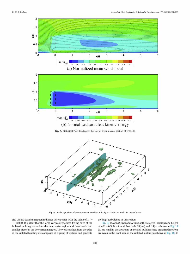
Fig. 7. Statistical Flow fields over the row of trees in cross section of y/H¼ 0.

Fig. 8. Bird's eye view of instantaneous vortices with λ2 ¼ �2000 around the row of trees.

Y. Qi, T. Ishihara Journal of Wind Engineering & Industrial Aerodynamics 177 (2018) 293–305

and the iso-surface in green indicates vortex cores with the value of λ2 ¼� 10000. It is clear that the large vortices generated by the edge of theisolated building move into the near wake region and then break intosmaller pieces in the downstream region. The vortices shed from the edgeof the isolated building are composed of a group of vortices and generate

300

the high turbulence in this region.Fig. 19 shows ΔSðuwÞ and ΔSðuvÞ at the selected locations and height

of z/H¼ 0.5. It is found that both ΔSðuwÞ and ΔSðuvÞ shown in Fig. 19(a) are small in the upstream of isolated building since organized motionsare weak in the front area of the isolated building as shown in Fig. 18. In

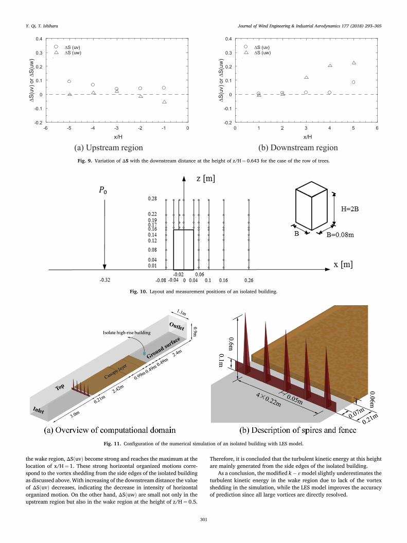
Fig. 11. Configuration of the numerical simulation of an isolated building with LES model.

Fig. 10. Layout and measurement positions of an isolated building.

Fig. 9. Variation of ΔS with the downstream distance at the height of z/H¼ 0.643 for the case of the row of trees.

Y. Qi, T. Ishihara Journal of Wind Engineering & Industrial Aerodynamics 177 (2018) 293–305

the wake region, ΔSðuvÞ become strong and reaches the maximum at thelocation of x/H¼ 1. These strong horizontal organized motions corre-spond to the vortex shedding from the side edges of the isolated buildingas discussed above. With increasing of the downstream distance the valueof ΔSðuvÞ decreases, indicating the decrease in intensity of horizontalorganized motion. On the other hand, ΔSðuwÞ are small not only in theupstream region but also in the wake region at the height of z/H¼ 0.5.

301

Therefore, it is concluded that the turbulent kinetic energy at this heightare mainly generated from the side edges of the isolated building.

As a conclusion, the modified k� εmodel slightly underestimates theturbulent kinetic energy in the wake region due to lack of the vortexshedding in the simulation, while the LES model improves the accuracyof prediction since all large vortices are directly resolved.

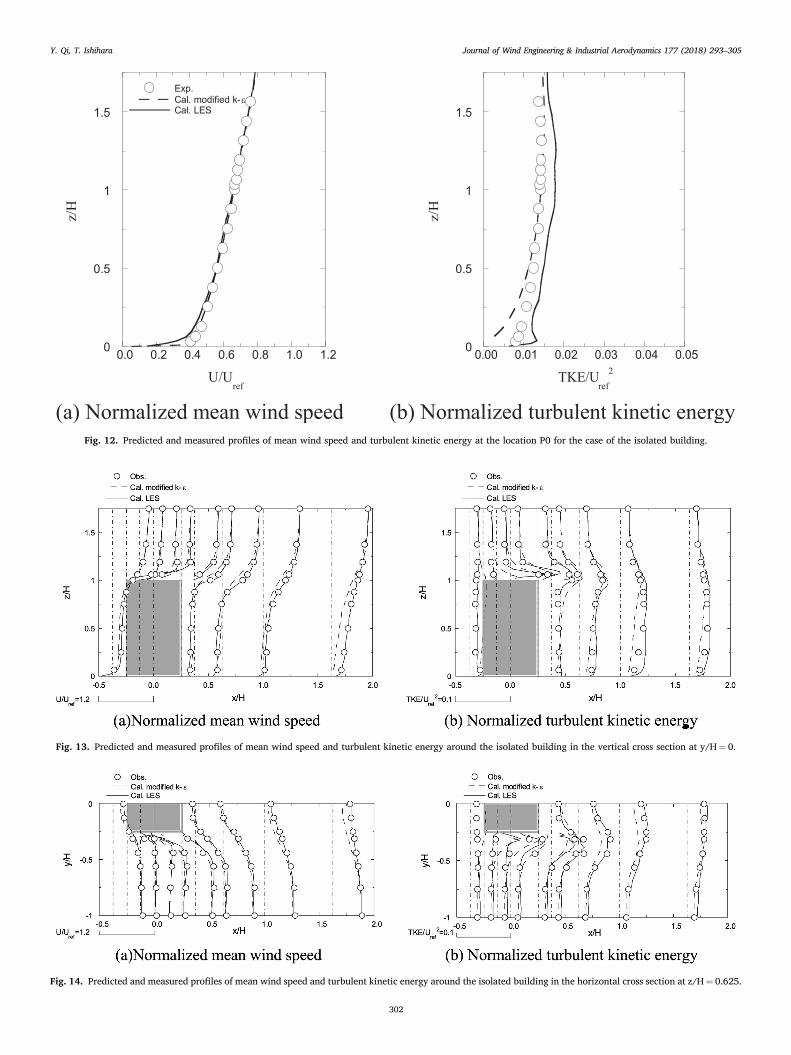
Fig. 14. Predicted and measured profiles of mean wind speed and turbulent kinetic energy around the isolated building in the horizontal cross section at z/H¼ 0.625.

Fig. 13. Predicted and measured profiles of mean wind speed and turbulent kinetic energy around the isolated building in the vertical cross section at y/H¼ 0.

Fig. 12. Predicted and measured profiles of mean wind speed and turbulent kinetic energy at the location P0 for the case of the isolated building.

Y. Qi, T. Ishihara Journal of Wind Engineering & Industrial Aerodynamics 177 (2018) 293–305

302

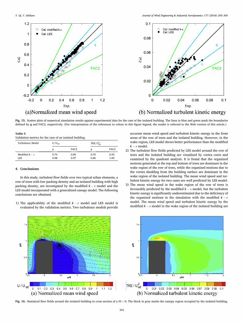
Fig. 15. Scatter plots of numerical simulation results against experimental data for the case of the isolated building. The lines in blue and green mark the boundariesdefined by q and FAC2, respectively. (For interpretation of the references to colour in this figure legend, the reader is referred to the Web version of this article.)

Table 5Validation metrics for the case of an isolated building.

Turbulence Model U=Uref TKE=U2ref

q FAC2 q FAC2

Modified k� ε 0.74 0.89 0.70 0.92LES 0.98 0.97 0.86 1.00

Y. Qi, T. Ishihara Journal of Wind Engineering & Industrial Aerodynamics 177 (2018) 293–305

4. Conclusions

In this study, turbulent flow fields over two typical urban elements, arow of trees with low packing density and an isolated building with highpacking density, are investigated by the modified k� ε model and theLES model incorporated with a generalized canopy model. The followingconclusions are obtained.

1) The applicability of the modified k� ε model and LES model isevaluated by the validation metrics. Two turbulence models provide

Fig. 16. Statistical flow fields around the isolated building in cross section of y/H¼

303

accurate mean wind speed and turbulent kinetic energy in the frontareas of the row of trees and the isolated building. However, in thewake region, LES model shows better performance than the modifiedk� ε model.

2) The turbulent flow fields predicted by LES model around the row oftrees and the isolated building are visualized by vortex cores andexamined by the quadrant analysis. It is found that the organizedmotions generated at the top and bottom of trees are dominant in thewake region of the row of trees, while the organized motions due tothe vortex shedding from the building surface are dominant in thewake region of the isolated building. The mean wind speed and tur-bulent kinetic energy for two cases are well predicted by LES model.

3) The mean wind speed in the wake region of the row of trees isfavourably predicted by the modified k� ε model, but the turbulentkinetic energy is significantly underestimated due to the deficiency ofthe organized motions in the simulation with the modified k� εmodel. The mean wind speed and turbulent kinetic energy by themodified k� ε model in the wake region of the isolated building are

0. The block in gray marks the canopy region occupied by the isolated building.

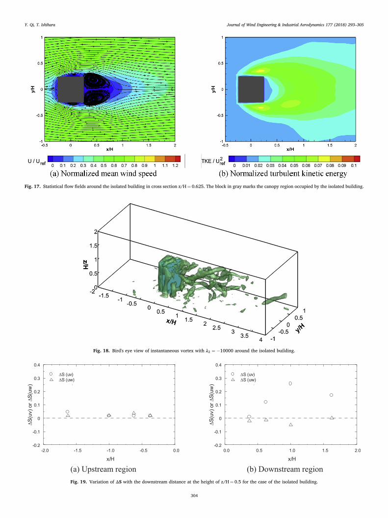
Fig. 18. Bird's eye view of instantaneous vortex with λ2 ¼ �10000 around the isolated building.

Fig. 19. Variation of ΔS with the downstream distance at the height of z/H¼ 0.5 for the case of the isolated building.

Fig. 17. Statistical flow fields around the isolated building in cross section z/H¼ 0.625. The block in gray marks the canopy region occupied by the isolated building.

Y. Qi, T. Ishihara Journal of Wind Engineering & Industrial Aerodynamics 177 (2018) 293–305

304

Y. Qi, T. Ishihara Journal of Wind Engineering & Industrial Aerodynamics 177 (2018) 293–305

also slightly underestimated due to lack of the vortex shedding in thewake region.

References

Aumond, P., Masson, V., Lac, C., Gauvreau, B., Dupont, S., Berengier, M., 2013. Includingthe drag effects of canopies: real case large-eddy simulation studies. Boundary-LayerMeteorol. 146 (1), 65–80.

Bailey, B.N., Stoll, R., 2013. Turbulence in sparse, organized vegetative canopies: a large-eddy simulation study. Boundary-Layer Meteorol. 147 (3), 369–400.

Blocken, B., Stathopoulos, T., Carmeliet, J., 2007. CFD simulation of the atmosphericboundary layer: wall function problems. Atmos. Environ. 41 (2), 238–252.

Blocken, B., Janssen, W., van Hooff, T., 2012. CFD simulation for pedestrian wind comfortand wind safety in urban areas: general decision framework and case study for theEindhoven University campus. Environ. Model. Software 30, 15–34.

Cheng, W.-C., Port�e-Agel, F., 2015. Adjustment of turbulent boundary-layer flow toidealized urban surfaces: a large-eddy simulation study. Boundary-Layer Meteorol.155 (2), 249–270.

Enoki, K., Ishihara, T., 2012. A generalized canopy model and its application to theprediction of urban wind climate. J. Jpn. Soci. Civ. Eng. Ser. A1 (Struct. Eng. Earthq.Eng) 68 (1), 28–47 (In Japanese).

Enoki, K., Ishihara, T., Yamaguchi, A., 2009. A generalized canopy model for the windprediction in the forest and the urban area. In: Proc. Of EWEC 2009.

Gousseau, P., Blocken, B., Stathopoulos, T., Van Heijst, G., 2011. CFD simulation of near-field pollutant dispersion on a high-resolution grid: a case study by LES and RANS fora building group in downtown Montreal. Atmos. Environ. 45 (2), 428–438.

Gousseau, P., Blocken, B., Van Heijst, G., 2013. Quality assessment of large-eddysimulation of wind flow around a high-rise building: validation and solutionverification. Comput. Fluids 79, 120–133.

Green, S., 1992. Modelling turbulent air flow in a stand of widely-spaced trees. Phoenics J5 (3), 294–312.

IEC 61400-2, I., 2006. Wind Turbines–part 2: Design Requirements for Small WindTurbines.

Irwin, H., 1979. Design and use of spires for natural wind simulation. National ResearchCouncil, Canada. LTR-LA-233.

Iwata, T., Kimura, A., Mochida, A., Yoshino, H., 2004. Optimization of tree canopy modelfor CFD prediction of wind environment at pedestran level. In: Proceedings ofNational Symposium on Wind Engineering (In Japanese).

Jeong, J., Hussain, F., 1995. On the identification of a vortex. J. Fluid Mech. 285, 69–94.Kato, M., 1993. The modeling of turbulent flow around stationary and vibrating square

cylinders. In: Ninth Symposium on Turbulent Shear Flows, 1993.Kida, S., Miura, H., 1998. Identification and analysis of vortical structures. Eur. J. Mech. B

Fluid 17 (4), 471–488.Kurotani, Y., Kiyota, N., Kobayashi, S., 2001. Windbreak effect of tsuijimatsu in Izumo:

Part 2. In: Proceedings of Architectural Institute of Japan, pp. 745–746.Liu, J., Chen, J., Black, T., Novak, M., 1996. E-εmodelling of turbulent air flow downwind

of a model forest edge. Boundary-Layer Meteorol. 77 (1), 21–44.

305

Lopes, A.S., Palma, J., Lopes, J.V., 2013. Improving a two-equation turbulence model forcanopy flows using large-eddy simulation. Boundary-Layer Meteorol. 149 (2),231–257.

Maruyama, T., 1993. Optimization of roughness parameters for staggered arrayed cubicblocks using experimental data. J. Wind Eng. Ind. Aerod. 46, 165–171.

Meng, Y., Hibi, K., 1998. Turbulent measurements of the flow field around a high-risebuilding. J. Wind Eng. 1998 (76), 55–64 (In Japanese).

Mochida, A., Tominaga, Y., Murakami, S., Yoshie, R., Ishihara, T., Ooka, R., 2002.Comparison of various k-ε models and DSM applied to flow around a high-risebuilding - report on AIJ cooperative project for CFD prediction of wind environment.Wind Struct. 5 (2–4), 227–244.

Mochida, A., Tabata, Y., Iwata, T., Yoshino, H., 2008. Examining tree canopy models forCFD prediction of wind environment at pedestrian level. J. Wind Eng. Ind. Aerod. 96(10), 1667–1677.

Mueller, E., Mell, W., Simeoni, A., 2014. Large eddy simulation of forest canopy flow forwildland fire modeling. Can. J. For. Res. 44 (12), 1534–1544.

Oikawa, S., Meng, Y., 1995. Turbulence characteristics and organized motion in asuburban roughness sublayer. Boundary-Layer Meteorol. 74 (3), 289–312.

Oka, S., Ishihara, T., 2009. Numerical study of aerodynamic characteristics of a squareprism in a uniform flow. J. Wind Eng. Ind. Aerod. 97 (11), 548–559.

Philips, D., Rossi, R., Iaccarino, G., 2013. Large-eddy simulation of passive scalardispersion in an urban-like canopy. J. Fluid Mech. 723, 404–428.

Rodi, W., 1997. Comparison of LES and RANS calculations of the flow around bluffbodies. J. Wind Eng. Ind. Aerod. 69, 55–75.

Salim, M.H., Schlünzen, K.H., Grawe, D., 2015. Including trees in the numericalsimulations of the wind flow in urban areas: should we care? J. Wind Eng. Ind. Aerod.144, 84–95.

Schatzmann, M., Olesen, H., Franke, J., 2010. COST 732 Model Evaluation Case Studies:Approach and Results, 121 pp. COST Office Brussels, ISBN, p. 3–00.

Suzuki, J., Yoshida, S., Ooka, R., Kurotani, Y., 2002. Study on windbreak effect ofTsujimatsu in Izumo using CFD analysis. In: Summaries of Technical Papers of AnnulMeeting Architectural Institute of Japan 2002 (In Japanese).

Tominaga, Y., Mochida, A., Murakami, S., Sawaki, S., 2008. Comparison of variousrevised k–εmodels and LES applied to flow around a high-rise building model with 1:1: 2 shape placed within the surface boundary layer. J. Wind Eng. Ind. Aerod. 96 (4),389–411.

Wilson, J., 1988. A second-order closure model for flow through vegetation. Boundary-Layer Meteorol. 42 (4), 371–392.

Xie, Z., Castro, I.P., 2006. LES and RANS for turbulent flow over arrays of wall-mountedobstacles. Flow, Turbul. Combust. 76 (3), 291–312.

Yang, B., Raupach, M.R., Shaw, R.H., Paw U, K.T., Morse, A.P., 2006. Large-eddysimulation of turbulent flow across a forest edge. Part I: flow statistics. Boundary-Layer Meteorol. 120 (3), 377–412.

Yoshie, R., Mochida, A., Tominaga, Y., Kataoka, H., Harimoto, K., Nozu, T., Shirasawa, T.,2007. Cooperative project for CFD prediction of pedestrian wind environment in theArchitectural Institute of Japan. J. Wind Eng. Ind. Aerod. 95 (9), 1551–1578.

Yoshie, R., Jiang, G., Shirasawa, T., Chung, J., 2011. CFD simulations of gas dispersionaround high-rise building in non-isothermal boundary layer. J. Wind Eng. Ind. Aerod.99 (4), 279–288.