Island biogeography

Key concepts

• Colonization-extinction balance

• Island-biogeography theory

Introduction

At the end of the last chapter, it was suggested that another mecha-

nism for the maintenance of α-diversity is the phenomenon of colonization-

extinction balance. Colonization-extinction balance refers to the fact

that the number of species at a site changes only through colonization

(or – much more rarely – local speciation), which results in an increase

in the number of species, and extinction, which results in a decrease in

the number of species. If the processes of colonization and extinction

are “balanced” then the number of species will be at an equilibrium.

Colonization-extinction balance is not a local mechanism per se be-

cause it reflects the combination of a local process (extinction) and a

process that depends on the state of surrounding ecosystems as well

(colonization). Thus, colonization-extinction balance is a process that

links α- and γ-diversity.

Figure 1: The Theory of IslandBiogeography by Robert MacArthurand E.O. Wilson.

Island biogeography theory

The process of colonization-extinction balance first received wide at-

tention in association with the development of island biogeography

theory by Robert MacArthur and E.O. Wilson. Island biogeography

theory aims to explain why islands have the number of species that

they do, both in relation to the mainland and in relation to other is-

lands. This model made both quantitative and qualitative predictions

about both the accumulation of species on an island over time and the

equilibrium number of species. It therefore generated a tremendous

amount of empirical work in the following decades to test and refine

the theory for use in specific contexts.

2

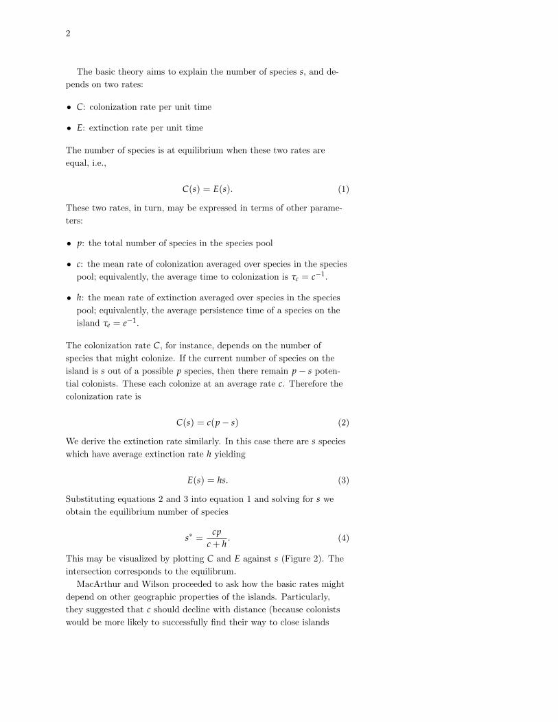
The basic theory aims to explain the number of species s, and de-

pends on two rates:

• C: colonization rate per unit time

• E: extinction rate per unit time

The number of species is at equilibrium when these two rates are

equal, i.e.,

C(s) = E(s). (1)

These two rates, in turn, may be expressed in terms of other parame-

ters:

• p: the total number of species in the species pool

• c: the mean rate of colonization averaged over species in the species

pool; equivalently, the average time to colonization is τc = c−1.

• h: the mean rate of extinction averaged over species in the species

pool; equivalently, the average persistence time of a species on the

island τe = e−1.

The colonization rate C, for instance, depends on the number of

species that might colonize. If the current number of species on the

island is s out of a possible p species, then there remain p − s poten-

tial colonists. These each colonize at an average rate c. Therefore the

colonization rate is

C(s) = c(p − s) (2)

We derive the extinction rate similarly. In this case there are s species

which have average extinction rate h yielding

E(s) = hs. (3)

Substituting equations 2 and 3 into equation 1 and solving for s we

obtain the equilibrium number of species

s∗ =cp

c + h. (4)

This may be visualized by plotting C and E against s (Figure 2). The

intersection corresponds to the equilibrum.

MacArthur and Wilson proceeded to ask how the basic rates might

depend on other geographic properties of the islands. Particularly,

they suggested that c should decline with distance (because colonists

would be more likely to successfully find their way to close islands

3

0 20 40 60 80 100

02

46

810

Species

Col

oniz

atio

n ra

te

02

46

810

Ext

inct

ion

rate

Figure 2: The basic model of island

biogeography predicts that speciesnumber on islands is determined by

the balance of colonization (black)

and extinction (blue). The equilib-rium (s∗ = 50) is indicated by the

vertical dashed line. Parameters of

this model are h = 0.1, c = 0.1, andp = 100.

than distant islands) and that e should decline with island size (be-

cause larger islands would support larger populations less vulnerable

to extinction). Including these factors requires introducing a few more

parameters:

• d: the distance of the island from the mainland (the presumed

source of colonists)

• a: the area of the island

• φ: a fit parameter governing the distance decay of colonization rate

• ε: a fit parameter governing the effect of area on extinction

For colonization, we suppose that the rate c(p − s) is the maximum

rate that applies in the extreme case where an island is directly adja-

cent to the mainland. For other islands, this must be discounted by

a factor that depends on the distance, i.e. we multiple c(p − s) by a

quantity that is one when d = 0 but approaches zero as d gets large.

Here, we assume this factor is an exponential decay, as if potential

colonists are “falling off” at a constant rate φ the further the island is

from the mainland. Accordingly, our new colonization rate is

C(s) = c(p − s)e−φd. (5)

For extinction, we derive a similar quantity. However, in this case

rather than thinking of an attrition process we refer to theoretical re-

sults showing that demographic fluctuations cause density-dependent

4

populations near their carrying capacities to have logarithms of ex-

tinction time proportional to carrying capacity (k). Assuming carrying

capacity is proportional to island area (k ∝ a), we have

E(s) = se−εa. (6)

In this case, the extinction rate goes to zero as the area gets large

(ecologically plausible if fluctuations are due to demographic fluctua-

tions, but not major disturbances like hurricanes). Additionally, the

total extinction rate diverges (goes to ∞) as area goes to zero, which

is also ecologically plausible: an island of area zero cannot support

even one species! Thus, we no longer have need for the variable h. As

before, we solve for the equilibium number of species:

s∗ =cpeεa

ceεa + eφd . (7)

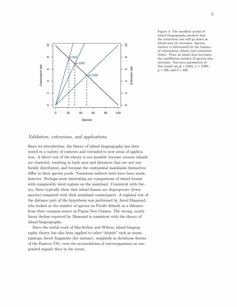
One qualitative prediction of this model is that the number of species

on islands will be directly proportional to p, the size of the species

pool on the associated mainland. Other predictions are perhaps eas-

ier to see graphically (Figures 3 and 4). First, concerning distance

to mainland, as the distance increases (different black lines in Figure

3), the equilibrium number of species declines. By contrast, the equi-

librium number of species increases with area (different blue lines in

Figure 4).

0 20 40 60 80 100

02

46

810

Species

Col

oniz

atio

n ra

te

02

46

810

Ext

inct

ion

rate

d=10,000

d=2000d=100

Figure 3: The modified model of is-

land biogeography predicts that thecolonization rate will go down as dis-

tance to the mainland (d) increases.

Species number is determined by thebalance of colonization (black) and

extinction (blue). Thus, as distance

to mainland increases, the equilibriumnumber of species decreases. Non-

distance parameters of this model are

φ = 0.0001, ε = 0.001, p = 100, anda = 2300.

5

0 20 40 60 80 100

02

46

810

Species

Col

oniz

atio

n ra

te

02

46

810

Ext

inct

ion

rate

a=2300

a=1000

a=500

Figure 4: The modified model of

island biogeography predicts thatthe extinction rate will go down as

island area (a) increases. Species

number is determined by the balanceof colonization (black) and extinction

(blue). Thus, as island area increases,

the equilibrium number of species alsoincreases. Non-area parameters of

this model are φ = 0.001, ε = 0.001,

p = 100, and d = 100.

Validation, extensions, and applications

Since its introduction, the theory of island biogeography has been

tested in a variety of contexts and extended to new areas of applica-

tion. A direct test of the theory is not possible because oceanic islands

are clustered, resulting in both area and distances that are not uni-

formly distributed, and because the continental mainlands themselves

differ in their species pools. Numerous indirect tests have been made,

however. Perhaps most interesting are comparisons of island faunas

with comparably sized regions on the mainland. Consistent with the-

ory, these typically show that island faunas are depauperate (fewer

species) compared with their mainland counterparts. A regional test of

the distance part of the hypothesis was performed by Jared Diamond,

who looked at the number of species on Pacific Islands as a distance

from their common source in Papua New Guinea. The strong, nearly

linear decline reported by Diamond is consistent with the theory of

island biogeography.

Since the initial work of MacArthur and Wilson, island biogeog-

raphy theory has also been applied to other “islands” such as moun-

taintops, forest fragments (for instance, songbirds in deciduous forests

of the Eastern US), even the accumulation of microorganisms on sus-

pended organic flocs in the ocean.

6

Homework

1. Derive equation 6 from the arguments in the paragraph preceding

it in the text.

2. Sketch the equilibrium number of species given by the island bio-

geography theory (i.e., equation 7) as (i) a function of area, and (ii)

a function of distance from the mainland.

Regional species diversity

Key concepts

• Two principles of species-area relationships

• Species area curve

Introduction

The previous chapter introduced MacArthur and Wilson’s theory of is-

land biogeography as an explanation for the maintenance of α-diversity

as a result of the interplay between a local process (extinction) and

a regional process (colonization). One feature of that theory was

that the equilibrium number of species on an oceanic island would

increase with the area of that island. Martin1 investigated this pat- 1 Jl Martin. Impoverishment ofisland bird communities in a Finnish

archipelago. Ornis Scandinavica, 14

(1):66–77, 1983

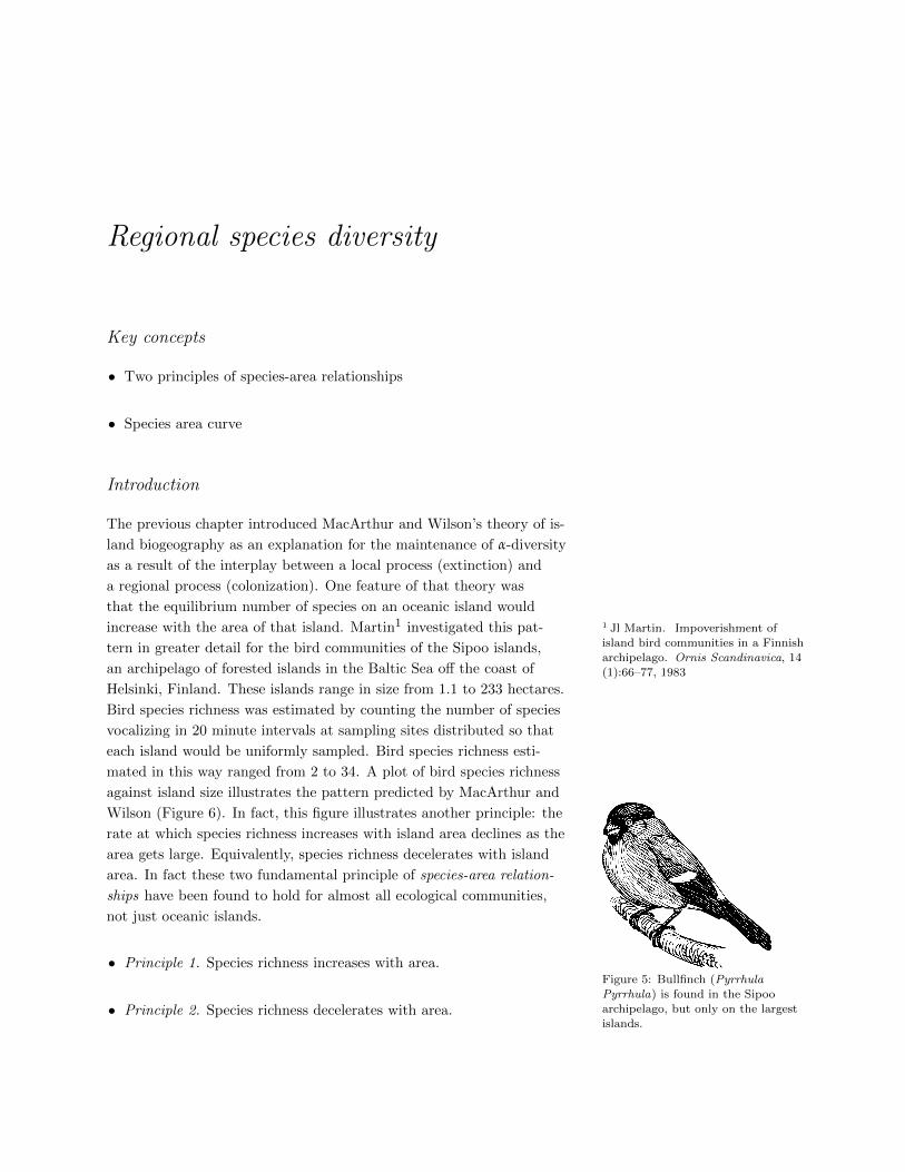
tern in greater detail for the bird communities of the Sipoo islands,

an archipelago of forested islands in the Baltic Sea off the coast of

Helsinki, Finland. These islands range in size from 1.1 to 233 hectares.

Bird species richness was estimated by counting the number of species

vocalizing in 20 minute intervals at sampling sites distributed so that

each island would be uniformly sampled. Bird species richness esti-

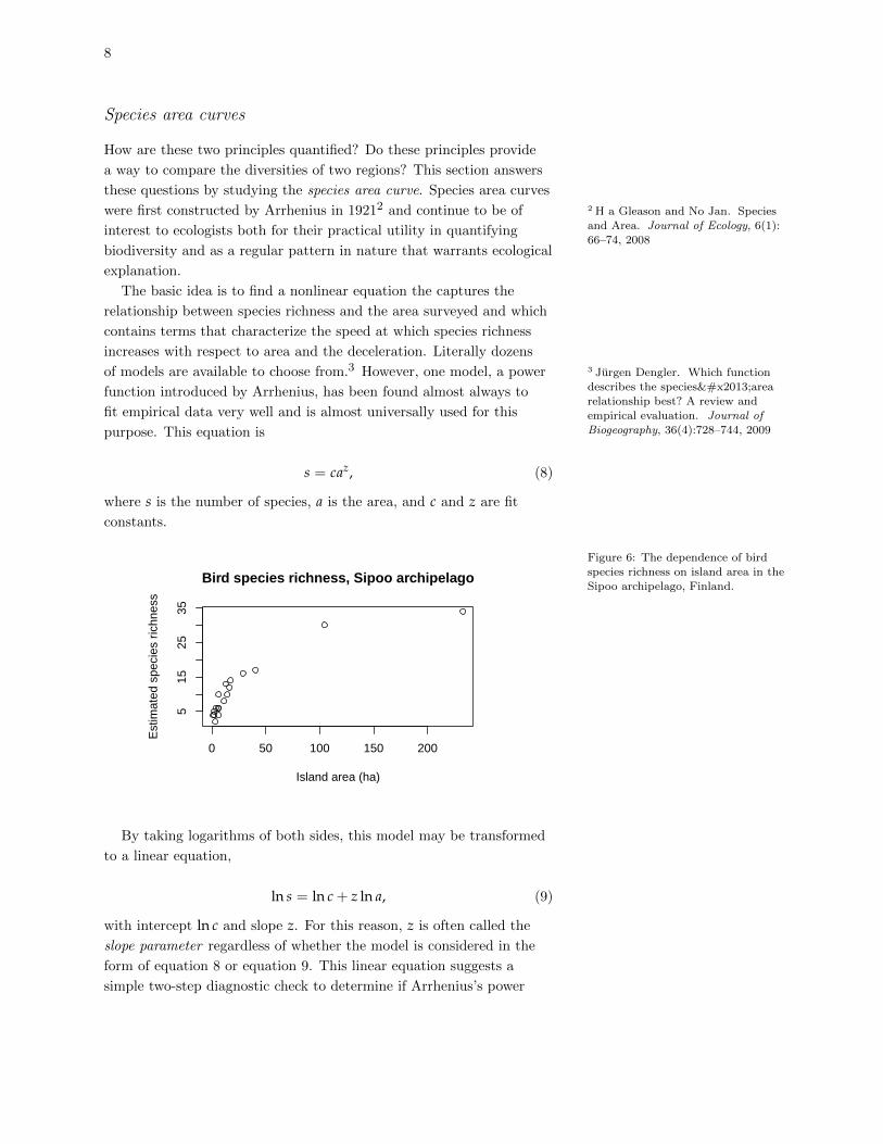
mated in this way ranged from 2 to 34. A plot of bird species richness

against island size illustrates the pattern predicted by MacArthur and

Wilson (Figure 6). In fact, this figure illustrates another principle: the

rate at which species richness increases with island area declines as the

area gets large. Equivalently, species richness decelerates with island

area. In fact these two fundamental principle of species-area relation-

ships have been found to hold for almost all ecological communities,

not just oceanic islands.

Figure 5: Bullfinch (Pyrrhula

Pyrrhula) is found in the Sipooarchipelago, but only on the largest

islands.

• Principle 1. Species richness increases with area.

• Principle 2. Species richness decelerates with area.

8

Species area curves

How are these two principles quantified? Do these principles provide

a way to compare the diversities of two regions? This section answers

these questions by studying the species area curve. Species area curves

were first constructed by Arrhenius in 19212 and continue to be of 2 H a Gleason and No Jan. Species

and Area. Journal of Ecology, 6(1):66–74, 2008

interest to ecologists both for their practical utility in quantifying

biodiversity and as a regular pattern in nature that warrants ecological

explanation.

The basic idea is to find a nonlinear equation the captures the

relationship between species richness and the area surveyed and which

contains terms that characterize the speed at which species richness

increases with respect to area and the deceleration. Literally dozens

of models are available to choose from.3 However, one model, a power 3 Jurgen Dengler. Which functiondescribes the species–area

relationship best? A review and

empirical evaluation. Journal ofBiogeography, 36(4):728–744, 2009

function introduced by Arrhenius, has been found almost always to

fit empirical data very well and is almost universally used for this

purpose. This equation is

s = caz, (8)

where s is the number of species, a is the area, and c and z are fit

constants.

0 50 100 150 200

515

2535

Bird species richness, Sipoo archipelago

Island area (ha)

Est

imat

ed s

peci

es r

ichn

ess

Figure 6: The dependence of birdspecies richness on island area in the

Sipoo archipelago, Finland.

By taking logarithms of both sides, this model may be transformed

to a linear equation,

ln s = ln c + z ln a, (9)

with intercept ln c and slope z. For this reason, z is often called the

slope parameter regardless of whether the model is considered in the

form of equation 8 or equation 9. This linear equation suggests a

simple two-step diagnostic check to determine if Arrhenius’s power

9

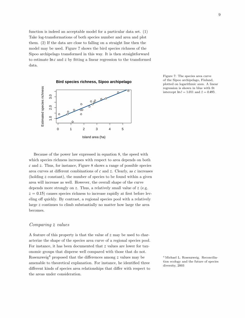
function is indeed an acceptable model for a particular data set. (1)

Take log-transformations of both species number and area and plot

them. (2) If the data are close to falling on a straight line then the

model may be used. Figure 7 shows the bird species richness of the

Sipoo archipelago transformed in this way. It is then straightforward

to estimate ln c and z by fitting a linear regression to the transformed

data.

0 1 2 3 4 5

1.0

2.0

3.0

Bird species richness, Sipoo archipelago

Island area (ha)

Est

imat

ed s

peci

es r

ichn

ess

Figure 7: The species area curveof the Sipoo archipelago, Finland,

plotted on logarithmic axes. A linear

regression is shown in blue with fitintercept ln c = 1.011 and z = 0.493.

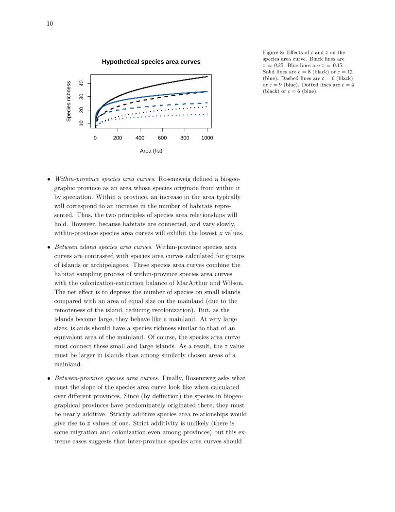
Because of the power law expressed in equation 8, the speed with

which species richness increases with respect to area depends on both

c and z. Thus, for instance, Figure 8 shows a range of possible species

area curves at different combinations of c and z. Clearly, as c increases

(holding z constant), the number of species to be found within a given

area will increase as well. However, the overall shape of the curve

depends more strongly on z. Thus, a relatively small value of z (e.g.

z = 0.15) causes species richness to increase rapidly at first before lev-

eling off quickly. By contrast, a regional species pool with a relatively

large z continues to climb substantially no matter how large the area

becomes.

Comparing z values

A feature of this property is that the value of z may be used to char-

acterize the shape of the species area curve of a regional species pool.

For instance, it has been documented that z values are lower for tax-

onomic groups that disperse well compared with those that do not.

Rosenzweig4 proposed that the differences among z values may be 4 Michael L. Rosenzweig. Reconcilia-tion ecology and the future of species

diversity, 2003amenable to theoretical explanation. For instance, he identified three

different kinds of species area relationships that differ with respect to

the areas under consideration.

10

0 200 400 600 800 1000

1020

3040

Hypothetical species area curves

Area (ha)

Spe

cies

ric

hnes

s

Figure 8: Effects of c and z on the

species area curve. Black lines arez = 0.25. Blue lines are z = 0.15.

Solid lines are c = 8 (black) or c = 12(blue). Dashed lines are c = 6 (black)or c = 9 (blue). Dotted lines are c = 4(black) or c = 6 (blue).

• Within-province species area curves. Rosenzweig defined a biogeo-

graphic province as an area whose species originate from within it

by speciation. Within a province, an increase in the area typically

will correspond to an increase in the number of habitats repre-

sented. Thus, the two principles of species area relationships will

hold. However, because habitats are connected, and vary slowly,

within-province species area curves will exhibit the lowest x values.

• Between island species area curves. Within-province species area

curves are contrasted with species area curves calculated for groups

of islands or archipelagoes. These species area curves combine the

habitat sampling process of within-province species area curves

with the colonization-extinction balance of MacArthur and Wilson.

The net effect is to depress the number of species on small islands

compared with an area of equal size on the mainland (due to the

remoteness of the island, reducing recolonization). But, as the

islands become large, they behave like a mainland. At very large

sizes, islands should have a species richness similar to that of an

equivalent area of the mainland. Of course, the species area curve

must connect these small and large islands. As a result, the z value

must be larger in islands than among similarly chosen areas of a

mainland.

• Between-province species area curves. Finally, Rosenzweg asks what

must the slope of the species area curve look like when calculated

over different provinces. Since (by definition) the species in biogeo-

graphical provinces have predominately originated there, they must

be nearly additive. Strictly additive species area relationships would

give rise to z values of one. Strict additivity is unlikely (there is

some migration and colonization even among provinces) but this ex-

treme cases suggests that inter-province species area curves should

11

have the largest z values.

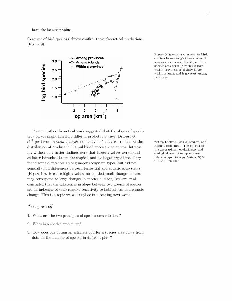
Censuses of bird species richness confirm these thoeretical predictions

(Figure 9).

Figure 9: Species area curves for birdsconfirm Rosenzweig’s three classes of

species area curves. The slope of the

species area curve (z value) is leastwithin provinces, is slightly larger

within islands, and is greatest among

provinces.

This and other theoretical work suggested that the slopes of species

area curves might therefore differ in predictable ways. Drakare et

al.5 performed a meta-analysis (an analyis-of-analyses) to look at the 5 Stina Drakare, Jack J. Lennon, andHelmut Hillebrand. The imprint of

the geographical, evolutionary and

ecological context on species-arearelationships. Ecology Letters, 9(2):

215–227, feb 2006

distribution of z values in 794 published species area curves. Interest-

ingly, their only major findings were that larger z values were found

at lower latitudes (i.e. in the tropics) and by larger organisms. They

found some differences among major ecosystem types, but did not

generally find differences between terrestrial and aquatic ecosystems

(Figure 10). Because high z values means that small changes in area

may correspond to large changes in species number, Drakare et al.

concluded that the differences in slope between two groups of species

are an indicator of their relative sensitivity to habitat loss and climate

change. This is a topic we will explore in a reading next week.

Test yourself

1. What are the two principles of species area relations?

2. What is a species area curve?

3. How does one obtain an estimate of z for a species area curve from

data on the number of species in different plots?

12

Figure 10: Meta-analysis of Drakareet al. shows the effects of latitude and

body size on the z values of species

area curves.

Bibliography

Stina Drakare, Jack J. Lennon, and Helmut Hillebrand. The imprint of

the geographical, evolutionary and ecological context on species-area

relationships. Ecology Letters, 9(2):215–227, feb 2006.

H a Gleason and No Jan. Species and Area. Journal of Ecology, 6(1):

66–74, 2008.

Jurgen Dengler. Which function describes the species–area

relationship best? A review and empirical evaluation. Journal of

Biogeography, 36(4):728–744, 2009.

Jl Martin. Impoverishment of island bird communities in a Finnish

archipelago. Ornis Scandinavica, 14(1):66–77, 1983.

Michael L. Rosenzweig. Reconciliation ecology and the future of

species diversity, 2003.

Chapter version: October 13, 2016