
Introduction to Statistics at DTUuniguld.dk/wp-content/guld/DTU/Statistik//2017-bog-eng.pdf ·...
416
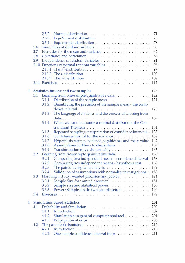
Introduction to Statistics at DTU 2017 Spring ¯ x Density n = 1 X ∼ N(0, 1) ¯ x Density n = 5 X ∼ U(0, 1) ¯ x n = 30 Density X ∼ Exp(1) ¯ X ∼ N μ, σ √ n
Transcript of Introduction to Statistics at DTUuniguld.dk/wp-content/guld/DTU/Statistik//2017-bog-eng.pdf ·...

Introduction to Statisticsat DTU
2017 Spring
x
Den
sity
x
Den
sity
n = 1
X ∼ N(0, 1)
x
Den
sity
x
Den
sity
x
Den
sity
x
Den
sity
n = 5
X ∼ U(0, 1)
x
Den
sity
x
Den
sity
x
Den
sity
x
n = 30
Den
sity
X ∼ Exp(1)
x
Den
sity
x
Den
sity
X ∼ N(
µ, σ√n
)
Chapter 0
Contents
1 Introduction, descriptive statistics, R and data visualization 11.1 What is Statistics - a primer . . . . . . . . . . . . . . . . . . . . . . 11.2 Statistics at DTU Compute . . . . . . . . . . . . . . . . . . . . . . . 31.3 Statistics - why, what, how? . . . . . . . . . . . . . . . . . . . . . . 41.4 Summary statistics . . . . . . . . . . . . . . . . . . . . . . . . . . . 8
1.4.1 Measures of centrality . . . . . . . . . . . . . . . . . . . . . 91.4.2 Measures of variability . . . . . . . . . . . . . . . . . . . . . 131.4.3 Measures of relation: correlation and covariance . . . . . . 16
1.5 Introduction to R and RStudio . . . . . . . . . . . . . . . . . . . . . 201.5.1 Console and scripts . . . . . . . . . . . . . . . . . . . . . . . 211.5.2 Assignments and vectors . . . . . . . . . . . . . . . . . . . 211.5.3 Descriptive statistics . . . . . . . . . . . . . . . . . . . . . . 221.5.4 Use of R in the course and at the exam . . . . . . . . . . . . 24
1.6 Plotting, graphics - data visualisation . . . . . . . . . . . . . . . . 261.6.1 Frequency distributions and the histogram . . . . . . . . . 261.6.2 Cumulative distributions . . . . . . . . . . . . . . . . . . . 281.6.3 The box plot and the modified box plot . . . . . . . . . . . 291.6.4 The Scatter plot . . . . . . . . . . . . . . . . . . . . . . . . . 351.6.5 Bar plots and Pie charts . . . . . . . . . . . . . . . . . . . . 361.6.6 More plots in R? . . . . . . . . . . . . . . . . . . . . . . . . 38
1.7 Exercises . . . . . . . . . . . . . . . . . . . . . . . . . . . . . . . . . 39
2 Probability and simulation 422.1 Random variable . . . . . . . . . . . . . . . . . . . . . . . . . . . . 422.2 Discrete random variables . . . . . . . . . . . . . . . . . . . . . . . 45
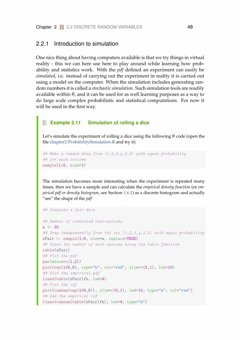
2.2.1 Introduction to simulation . . . . . . . . . . . . . . . . . . . 482.2.2 Mean and variance . . . . . . . . . . . . . . . . . . . . . . . 51
2.3 Discrete distributions . . . . . . . . . . . . . . . . . . . . . . . . . . 582.3.1 Binomial distribution . . . . . . . . . . . . . . . . . . . . . . 582.3.2 Hypergeometric distribution . . . . . . . . . . . . . . . . . 612.3.3 Poisson distribution . . . . . . . . . . . . . . . . . . . . . . 63
2.4 Continuous random variables . . . . . . . . . . . . . . . . . . . . . 672.4.1 Mean and Variance . . . . . . . . . . . . . . . . . . . . . . . 69
2.5 Continuous distributions . . . . . . . . . . . . . . . . . . . . . . . . 702.5.1 Uniform distribution . . . . . . . . . . . . . . . . . . . . . . 70
2.5.2 Normal distribution . . . . . . . . . . . . . . . . . . . . . . 712.5.3 Log-Normal distribution . . . . . . . . . . . . . . . . . . . . 782.5.4 Exponential distribution . . . . . . . . . . . . . . . . . . . . 78
2.6 Simulation of random variables . . . . . . . . . . . . . . . . . . . . 822.7 Identities for the mean and variance . . . . . . . . . . . . . . . . . 852.8 Covariance and correlation . . . . . . . . . . . . . . . . . . . . . . 882.9 Independence of random variables . . . . . . . . . . . . . . . . . . 912.10 Functions of normal random variables . . . . . . . . . . . . . . . . 96
2.10.1 The χ2-distribution . . . . . . . . . . . . . . . . . . . . . . . 972.10.2 The t-distribution . . . . . . . . . . . . . . . . . . . . . . . . 1022.10.3 The F-distribution . . . . . . . . . . . . . . . . . . . . . . . 108
2.11 Exercises . . . . . . . . . . . . . . . . . . . . . . . . . . . . . . . . . 112
3 Statistics for one and two samples 1223.1 Learning from one-sample quantitative data . . . . . . . . . . . . 122
3.1.1 Distribution of the sample mean . . . . . . . . . . . . . . . 1243.1.2 Quantifying the precision of the sample mean - the confi-
dence interval . . . . . . . . . . . . . . . . . . . . . . . . . . 1293.1.3 The language of statistics and the process of learning from
data . . . . . . . . . . . . . . . . . . . . . . . . . . . . . . . . 1323.1.4 When we cannot assume a normal distribution: the Cen-
tral Limit Theorem . . . . . . . . . . . . . . . . . . . . . . . 1343.1.5 Repeated sampling interpretation of confidence intervals . 1373.1.6 Confidence interval for the variance . . . . . . . . . . . . . 1383.1.7 Hypothesis testing, evidence, significance and the p-value 1423.1.8 Assumptions and how to check them . . . . . . . . . . . . 1573.1.9 Transformation towards normality . . . . . . . . . . . . . . 163
3.2 Learning from two-sample quantitative data . . . . . . . . . . . . 1673.2.1 Comparing two independent means - confidence Interval 1683.2.2 Comparing two independent means - hypothesis test . . . 1693.2.3 The paired design and analysis . . . . . . . . . . . . . . . . 1793.2.4 Validation of assumptions with normality investigations . 183
3.3 Planning a study: wanted precision and power . . . . . . . . . . . 1843.3.1 Sample Size for wanted precision . . . . . . . . . . . . . . . 1843.3.2 Sample size and statistical power . . . . . . . . . . . . . . . 1853.3.3 Power/Sample size in two-sample setup . . . . . . . . . . 190
3.4 Exercises . . . . . . . . . . . . . . . . . . . . . . . . . . . . . . . . . 192
4 Simulation Based Statistics 2024.1 Probability and Simulation . . . . . . . . . . . . . . . . . . . . . . . 202
4.1.1 Introduction . . . . . . . . . . . . . . . . . . . . . . . . . . . 2024.1.2 Simulation as a general computational tool . . . . . . . . . 2044.1.3 Propagation of error . . . . . . . . . . . . . . . . . . . . . . 206
4.2 The parametric bootstrap . . . . . . . . . . . . . . . . . . . . . . . 2104.2.1 Introduction . . . . . . . . . . . . . . . . . . . . . . . . . . . 2104.2.2 One-sample confidence interval for µ . . . . . . . . . . . . 211
4.2.3 One-sample confidence interval for any feature assumingany distribution . . . . . . . . . . . . . . . . . . . . . . . . . 213
4.2.4 Two-sample confidence intervals assuming any distribu-tions . . . . . . . . . . . . . . . . . . . . . . . . . . . . . . . 217
4.3 The non-parametric bootstrap . . . . . . . . . . . . . . . . . . . . . 2224.3.1 Introduction . . . . . . . . . . . . . . . . . . . . . . . . . . . 2224.3.2 One-sample confidence interval for µ . . . . . . . . . . . . 2224.3.3 One-sample confidence interval for any feature . . . . . . 2244.3.4 Two-sample confidence intervals . . . . . . . . . . . . . . . 225
4.4 Bootstrapping – a further perspective . . . . . . . . . . . . . . . . 2294.4.1 Non-parametric bootstrapping with the boot-package . . 230
4.5 Exercises . . . . . . . . . . . . . . . . . . . . . . . . . . . . . . . . . 239
5 Simple Linear regression 2445.1 Linear regression and least squares . . . . . . . . . . . . . . . . . . 2445.2 Parameter estimates and estimators . . . . . . . . . . . . . . . . . 247
5.2.1 Estimators are central . . . . . . . . . . . . . . . . . . . . . 2525.3 Variance of estimators . . . . . . . . . . . . . . . . . . . . . . . . . 2535.4 Distribution and testing of parameters . . . . . . . . . . . . . . . . 260
5.4.1 Confidence and prediction intervals for the line . . . . . . 2645.5 Matrix formulation of simple linear regression . . . . . . . . . . . 2675.6 Correlation . . . . . . . . . . . . . . . . . . . . . . . . . . . . . . . . 270
5.6.1 Inference on the sample correlation coefficient . . . . . . . 2715.6.2 Correlation and regression . . . . . . . . . . . . . . . . . . 272
5.7 Model validation . . . . . . . . . . . . . . . . . . . . . . . . . . . . 2745.8 Exercises . . . . . . . . . . . . . . . . . . . . . . . . . . . . . . . . . 278
6 Multiple Linear Regression 2856.1 Parameter estimation . . . . . . . . . . . . . . . . . . . . . . . . . . 287
6.1.1 Confidence and prediction intervals for the line . . . . . . 2926.2 Curvilinear regression . . . . . . . . . . . . . . . . . . . . . . . . . 2966.3 Collinearity . . . . . . . . . . . . . . . . . . . . . . . . . . . . . . . 2996.4 Residual analysis . . . . . . . . . . . . . . . . . . . . . . . . . . . . 3016.5 Linear regression in R . . . . . . . . . . . . . . . . . . . . . . . . . . 3046.6 Matrix formulation . . . . . . . . . . . . . . . . . . . . . . . . . . . 305
6.6.1 Confidence and prediction intervals for the line . . . . . . 3076.7 Exercises . . . . . . . . . . . . . . . . . . . . . . . . . . . . . . . . . 308
7 Inference for Proportions 3127.1 Categorical data . . . . . . . . . . . . . . . . . . . . . . . . . . . . . 3127.2 Estimation of single proportions . . . . . . . . . . . . . . . . . . . 312
7.2.1 Testing hypotheses . . . . . . . . . . . . . . . . . . . . . . . 3177.2.2 Sample size determination . . . . . . . . . . . . . . . . . . 320
7.3 Comparing proportions in two populations . . . . . . . . . . . . . 3217.4 Comparing several proportions . . . . . . . . . . . . . . . . . . . . 3267.5 Analysis of Contingency Tables . . . . . . . . . . . . . . . . . . . . 331
7.5.1 Comparing several groups . . . . . . . . . . . . . . . . . . 3317.5.2 Independence between the two categorical variables . . . 335
7.6 Exercises . . . . . . . . . . . . . . . . . . . . . . . . . . . . . . . . . 339
8 Comparing means of multiple groups - ANOVA 3438.1 Introduction . . . . . . . . . . . . . . . . . . . . . . . . . . . . . . . 3438.2 One-way ANOVA . . . . . . . . . . . . . . . . . . . . . . . . . . . . 344
8.2.1 Data structure and model . . . . . . . . . . . . . . . . . . . 3448.2.2 Decomposition of variability, the ANOVA table . . . . . . 3478.2.3 Post hoc comparisons . . . . . . . . . . . . . . . . . . . . . 3548.2.4 Model control . . . . . . . . . . . . . . . . . . . . . . . . . . 3588.2.5 A complete worked through example: plastic types for
lamps . . . . . . . . . . . . . . . . . . . . . . . . . . . . . . . 3608.3 Two-way ANOVA . . . . . . . . . . . . . . . . . . . . . . . . . . . . 364
8.3.1 Data structure and model . . . . . . . . . . . . . . . . . . . 3648.3.2 Decomposition of variability and the ANOVA table . . . . 3678.3.3 Post hoc comparisons . . . . . . . . . . . . . . . . . . . . . 3708.3.4 Model control . . . . . . . . . . . . . . . . . . . . . . . . . . 3728.3.5 A complete worked through example: Car tires . . . . . . 374
8.4 Perspective . . . . . . . . . . . . . . . . . . . . . . . . . . . . . . . . 3778.5 Exercises . . . . . . . . . . . . . . . . . . . . . . . . . . . . . . . . . 379
Glossaries 389
Acronyms 393
A Collection of formulas and R commands 394A.1 Introduction, descriptive statistics, R and data visualization . . . 394A.2 Probability and Simulation . . . . . . . . . . . . . . . . . . . . . . . 396
A.2.1 Distributions . . . . . . . . . . . . . . . . . . . . . . . . . . 398A.3 Statistics for one and two samples . . . . . . . . . . . . . . . . . . 402A.4 Simulation based statistics . . . . . . . . . . . . . . . . . . . . . . . 404A.5 Simple linear regression . . . . . . . . . . . . . . . . . . . . . . . . 405A.6 Multiple linear regression . . . . . . . . . . . . . . . . . . . . . . . 407A.7 Inference for proportions . . . . . . . . . . . . . . . . . . . . . . . . 408A.8 Comparing means of multiple groups - ANOVA . . . . . . . . . . 409
The plot on the front page is an illustration of the Central Limit Theorem (CLT). Toput it shortly, it states that when sampling a population: as the sample size increases,then the mean of the sample converges to a normal distribution – no matter the distri-bution of the population. The thumb rule is that the normal distribution can be usedfor the sample mean when the sample size n is above 30 observations (n is the numberobservations in the sample). The plot is created by simulating 100000 sample meansX = ∑n
i=1 Xi (where Xi is an observation from a distribution) and plotting their his-togram with the CLT distribution on top (the red linie). The upper is for the normal, themid is for the uniform and the lower is for the exponential distribution. We can thus see

that as n increase, then the distribution of the simulated sample means x approachesthe distribution stated by the CLT (it is the normal distribution X ∼ N
(µ, σ√
n
), where
µ is the mean and σ is the standard deviation of the population), see more in Section3.1.4.

Chapter 1 1
Chapter 1
Introduction, descriptive statistics, Rand data visualization
This is the first chapter in the eight-chapter DTU Introduction to Statistics book.It consists of eight chapters:
1. Introduction, descriptive statistics, R and data visualization
2. Probability and simulation
3. Statistical analysis of one and two sample data
4. Statistics by simulation
5. Simple linear regression
6. Multiple linear regression
7. Analysis of categorical data
8. Analysis of variance (analysis of multigroup data)
In this first chapter the idea of statistics is introduced together with some of thebasic summary statistics and data visualization methods. The software usedthroughout the book for working with statistics, probability and data analysis isthe open source environment R. An introduction to R is included in this chapter.
1.1 What is Statistics - a primer
To catch your attention we will start out trying to give an impression of theimportance of statistics in modern science and engineering.

Chapter 1 1.1 WHAT IS STATISTICS - A PRIMER 2
In the well respected New England Journal of medicine a millenium editorial onthe development of medical research in a thousand years was written:
EDITORIAL: Looking Back on the Millennium in Medicine, N Engl J Med, 342:42-49, January 6, 2000, NEJM200001063420108.
They came up with a list of 11 points summarizing the most important devel-opments for the health of mankind in a millenium:
• Elucidation of human anatomy and physiology
• Discovery of cells and their substructures
• Elucidation of the chemistry of life
• Application of statistics to medicine
• Development of anesthesia
• Discovery of the eelation of microbes to disease
• Elucidation of inheritance and genetics
• Knowledge of the immune system
• Development of body imaging
• Discovery of antimicrobial agents
• Development of molecular pharmacotherapy
The reason for showing the list here is pretty obvious: one of the points is Ap-plication of Statistics to Medicine! Considering the other points on the list, andwhat the state of medical knowledge was around 1000 years ago, it is obviouslya very impressive list of developments. The reasons for statistics to be on thislist are several and we mention two very important historical landmarks here.Quoting the paper:
"One of the earliest clinical trials took place in 1747, when James Lind treated 12scorbutic ship passengers with cider, an elixir of vitriol, vinegar, sea water, orangesand lemons, or an electuary recommended by the ship’s surgeon. The success of thecitrus-containing treatment eventually led the British Admiralty to mandate the provi-sion of lime juice to all sailors, thereby eliminating scurvy from the navy." (See alsoJames_Lind).
Still today, clinical trials, including the statistical analysis of the outcomes, aretaking place in massive numbers. The medical industry needs to do this inorder to find out if their new developed drugs are working and to provide doc-umentation to have them accepted for the World markets. The medical industryis probably the sector recruiting the highest number of statisticians among allsectors. Another quote from the paper:

Chapter 1 1.2 STATISTICS AT DTU COMPUTE 3
"The origin of modern epidemiology is often traced to 1854, when John Snow demon-strated the transmission of cholera from contaminated water by analyzing disease ratesamong citizens served by the Broad Street Pump in London’s Golden Square. He ar-rested the further spread of the disease by removing the pump handle from the pollutedwell." (See also John_Snow_(physician)).
Still today, epidemiology, both human and veterinarian, maintains to be an ex-tremely important field of research (and still using a lot of statistics). An im-portant topic, for instance, is the spread of diseases in populations, e.g. virusspreads like Ebola and others.
Actually, today more numbers/data than ever are being collected and the amountsare still increasing exponentially. One example is Internet data, that internetcompanies like Google, Facebook, IBM and others are using extensively. Aquote from New York Times, 5. August 2009, from the article titled “For To-day’s Graduate, Just One Word: Statistics” is:
“I keep saying that the sexy job in the next 10 years will be statisticians," said HalVarian, chief economist at Google. ‘and I’m not kidding.’ ”
The article ends with the following quote:
“The key is to let computers do what they are good at, which is trawling these massivedata sets for something that is mathematically odd,” said Daniel Gruhl, an I.B.M. re-searcher whose recent work includes mining medical data to improve treatment. “Andthat makes it easier for humans to do what they are good at - explain those anomalies.”
1.2 Statistics at DTU Compute
At DTU Compute at the Technical University of Denmark statistics is used,taught and researched mainly within four research sections:
• Statistics and Data Analysis
• Dynamical Systems
• Image Analysis & Computer Graphics
• Cognitive Systems
Each of these sections have their own focus area within statistics, modellingand data analysis. On the master level it is an important option within DTUCompute studies to specialize in statistics of some kind on the joint master pro-gramme in Mathematical Modelling and Computation (MMC). And a Statisti-cian is a wellknown profession in industry, research and public sector institu-tions.

Chapter 1 1.3 STATISTICS - WHY, WHAT, HOW? 4
The high relevance of the topic of statistics and data analysis today is also il-lustrated by the extensive list of ongoing research projects involving many anddiverse industrial partners within these four sections. Neither society nor in-dustry can cope with all the available data without using highly specialized per-sons in statistical techniques, nor can they cope and be internationally compet-itive without constinuosly further developing these methodologies in researchprojects. Statistics is and will continue to be a relevant, viable and dynamicfield. And the amount of experts in the field continues to be small comparedto the demand for experts, hence obtaining skills in statistics is for sure a wisecareer choice for an engineer. Still for any engineer not specialising in statistics,a basic level of statistics understanding and data handling ability is crucial forthe ability to navigate in modern society and business, which will be heavilyinfluenced by data of many kinds in the future.
1.3 Statistics - why, what, how?
Often in society and media, the word statistics is used simply as the name fora summary of some numbers, also called data, by means of a summary tableand/or plot. We also embrace this basic notion of statistics, but will call suchbasic data summaries descriptive statistics or explorative statistics. The meaningof statistics goes beyond this and will rather mean “how to learn from data in aninsightful way and how to use data for clever decision making”, in short we call thisinferential statistics. This could be on the national/societal level, and could berelated to any kind of topic, such as e.g. health, economy or environment, wheredata is collected and used for learning and decision making. For example:
• Cancer registries
• Health registries in general
• Nutritional databases
• Climate data
• Macro economic data (Unemployment rates, GNP etc. )
• etc.
The latter is the type of data that historically gave name to the word statistics. Itoriginates from the Latin ‘statisticum collegium’ (state advisor) and the Italianword ‘statista’ (statesman/politician). The word was brought to Denmark bythe Gottfried Achenwall from Germany in 1749 and originally described theprocessing of data for the state, see also History_of_statistics.
Or it could be for industrial and business applications:
Chapter 1 1.3 STATISTICS - WHY, WHAT, HOW? 5
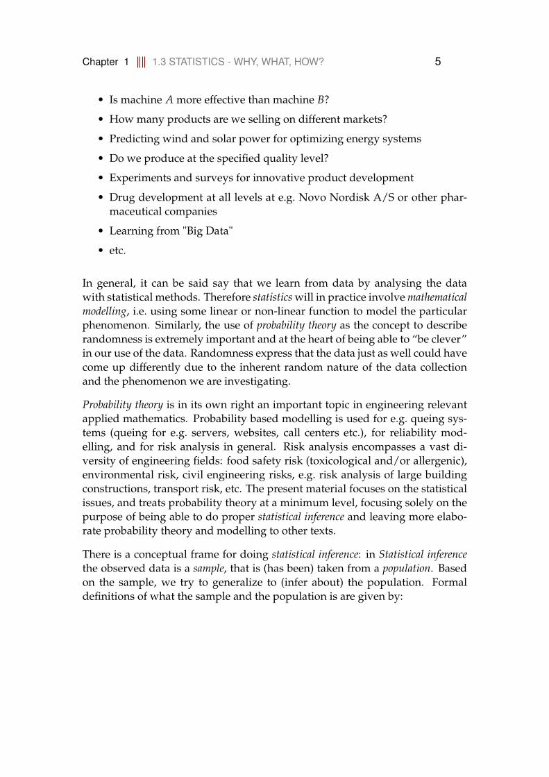
• Is machine A more effective than machine B?
• How many products are we selling on different markets?
• Predicting wind and solar power for optimizing energy systems
• Do we produce at the specified quality level?
• Experiments and surveys for innovative product development
• Drug development at all levels at e.g. Novo Nordisk A/S or other phar-maceutical companies
• Learning from "Big Data"
• etc.
In general, it can be said say that we learn from data by analysing the datawith statistical methods. Therefore statistics will in practice involve mathematicalmodelling, i.e. using some linear or non-linear function to model the particularphenomenon. Similarly, the use of probability theory as the concept to describerandomness is extremely important and at the heart of being able to “be clever”in our use of the data. Randomness express that the data just as well could havecome up differently due to the inherent random nature of the data collectionand the phenomenon we are investigating.
Probability theory is in its own right an important topic in engineering relevantapplied mathematics. Probability based modelling is used for e.g. queing sys-tems (queing for e.g. servers, websites, call centers etc.), for reliability mod-elling, and for risk analysis in general. Risk analysis encompasses a vast di-versity of engineering fields: food safety risk (toxicological and/or allergenic),environmental risk, civil engineering risks, e.g. risk analysis of large buildingconstructions, transport risk, etc. The present material focuses on the statisticalissues, and treats probability theory at a minimum level, focusing solely on thepurpose of being able to do proper statistical inference and leaving more elabo-rate probability theory and modelling to other texts.
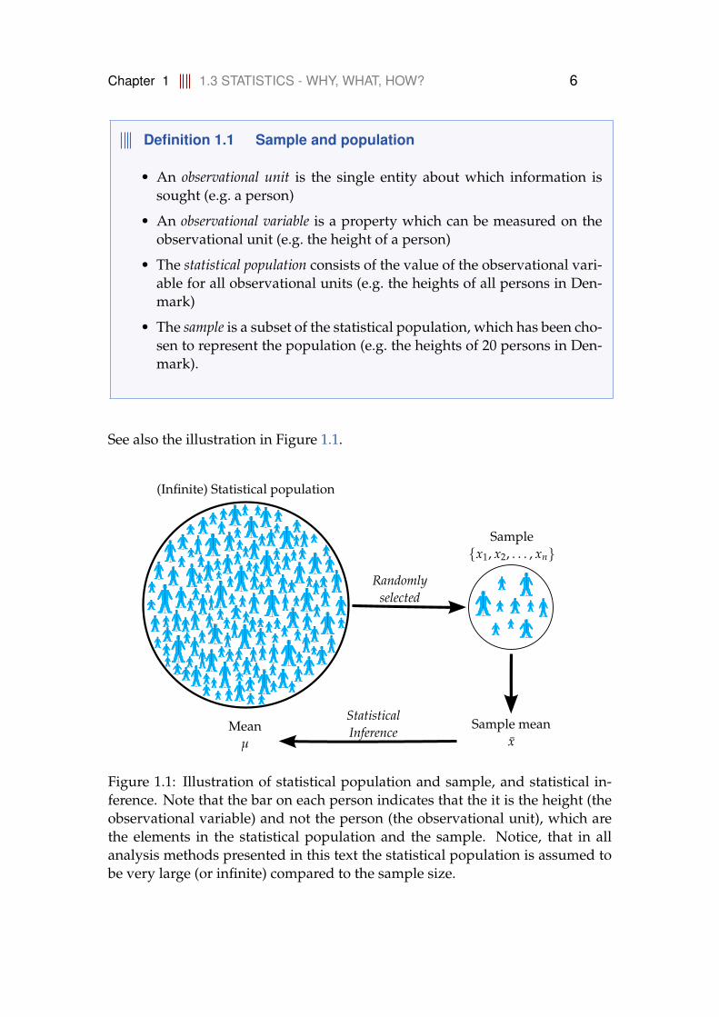
There is a conceptual frame for doing statistical inference: in Statistical inferencethe observed data is a sample, that is (has been) taken from a population. Basedon the sample, we try to generalize to (infer about) the population. Formaldefinitions of what the sample and the population is are given by:
Chapter 1 1.3 STATISTICS - WHY, WHAT, HOW? 6
Definition 1.1 Sample and population
• An observational unit is the single entity about which information issought (e.g. a person)
• An observational variable is a property which can be measured on theobservational unit (e.g. the height of a person)
• The statistical population consists of the value of the observational vari-able for all observational units (e.g. the heights of all persons in Den-mark)
• The sample is a subset of the statistical population, which has been cho-sen to represent the population (e.g. the heights of 20 persons in Den-mark).
See also the illustration in Figure 1.1.
Randomlyselected
(Infinite) Statistical population
Sample meanx
Meanµ
Sample{x1, x2, . . . , xn}
StatisticalInference
Figure 1.1: Illustration of statistical population and sample, and statistical in-ference. Note that the bar on each person indicates that the it is the height (theobservational variable) and not the person (the observational unit), which arethe elements in the statistical population and the sample. Notice, that in allanalysis methods presented in this text the statistical population is assumed tobe very large (or infinite) compared to the sample size.

Chapter 1 1.3 STATISTICS - WHY, WHAT, HOW? 7
This is all a bit abstract at this point. And likely adding to the potential confu-sion about this is the fact that the words population and sample will have a “lessprecise” meaning when used in everyday language. When they are used in astatistical context the meaning is very specific, as given by the definition above.Let us consider a simple example:
Example 1.2
The following study is carried out (actual data collection): the height of 20 personsin Denmark is measured. This will give us 20 values x1, . . . , x20 in cm. The sampleis then simply these 20 values. The statistical population is the height values of allpeople in Denmark. The observational unit is a person.
The meaning of sample in statistics is clearly different from how a chemist ormedical doctor would use the word, where a sample would be the actual sub-stance in e.g. the petri dish. Within this book, when using the word sample, thenit is always in the statistical meaning i.e. a set of values taken from a statisticalpopulation.
With regards to the meaning of population within statistics the difference to theeveryday meaning is less obvious: but note that the statistical population in theexample is defined to be the height values of persons, not actually the persons.Had we measured the weights instead the statistical population would be quitedifferent. Also later we will realize that statistical populations in engineeringcontexts can refer to many other things than populations as in a group of or-ganisms, hence stretching the use of the word beyond the everyday meaning.From this point: population will be used instead of statistical population in orderto simplify the text.
The population in a given situation will be linked with the actual study and/orexperiment carried out - the data collection procedure sometimes also denotedthe data generating process. For the sample to represent relevant informationabout the population it should be representative for that population. In the ex-ample, had we only measured male heights, the population we can say any-thing about would be the male height population only, not the entire heightpopulation.
A way to achieve a representative sample is that each observation (i.e. eachvalue) selected from the population, is randomly and independently selected ofeach other, and then the sample is called a random sample.

Chapter 1 1.4 SUMMARY STATISTICS 8
1.4 Summary statistics
The descriptive part of studying data maintains to be an important part of statis-tics. This means that it is recommended to study the given data, the sample, bymeans of descriptive statistics as a first step, even though the purpose of a fullstatistical analysis is to eventually perform some of the new inferential toolstaught in this book, that will go beyond the pure descriptive part. The aims ofthe initial descriptive part are several, and when moving to more complex datasettings later in the book, it will be even more clear how the initial descriptivepart serves as a way to prepare for and guide yourself in the subsequent moreformal inferential statistical analysis.
The initial part is also called an explorative analysis of the data. We use a numberof summary statistics to summarize and describe a sample consisting of one ortwo variables:
• Measures of centrality:
– Mean
– Median
– Quantiles
• Measures of “spread”:
– Variance
– Standard deviation
– Coefficient of variation
– Inter Quartile Range (IQR)
• Measures of relation (between two variables):
– Covariance
– Correlation
One important point to notice is that these statistics can only be calculated forthe sample and not for the population - we simply don’t know all the valuesin the population! But we want to learn about the population from the sample.For example when we have a random sample from a population we say that thesample mean (x) is an estimate of the mean of the population, often then denotedµ, as illustrated in Figure 1.1.
Chapter 1 1.4 SUMMARY STATISTICS 9
Remark 1.3
Notice, that we put ’sample’ in front of the name of the statistic, when it iscalculated for the sample, but we don’t put ’population’ in front when werefer to it for the population (e.g. we can think of the mean as the true mean).
HOWEVER we don’t put sample in front of the name every time it shouldbe there! This is to keep the text simpler and since traditionally this is notstrictly done, for example the median is rarely called the sample median,even though it makes perfect sense to distinguish between the sample me-dian and the median (i.e. the population median). Further, it should beclear from the context if the statistic refers to the sample or the population,when it is not clear then we distinguish in the text. Most of the way we dodistinguish strictly for the mean, standard deviation, variance, covariance andcorrelation.
1.4.1 Measures of centrality
The sample mean is a key number that indicates the centre of gravity or center-ing of the sample. Given a sample of n observations x1, . . . , xn, it is defined asfollows:
Definition 1.4 Sample mean
The sample mean is the sum of observations divided by the number of ob-servations
x =1n
n
∑i=1
xi. (1-1)
Sometimes this is refered to as the average.
The median is also a key number indicating the center of sample (note that tobe strict we should call it ’sample median’, see Remark 1.3 above). In somecases, for example in the case of extreme values or skewed distributions, themedian can be preferable to the mean. The median is the observation in themiddle of the sample (in sorted order). One may express the ordered observa-tions as x(1), . . . , x(n), where then x(1) is the smallest of all x1, . . . , xn (also called
Chapter 1 1.4 SUMMARY STATISTICS 10
the minimum) and x(n) is the largest of all x1, . . . , xn (also called the maximum).
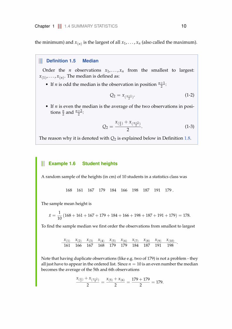
Definition 1.5 Median
Order the n observations x1, . . . , xn from the smallest to largest:x(1), . . . , x(n). The median is defined as:
• If n is odd the median is the observation in position n+12 :
Q2 = x( n+12 ). (1-2)
• If n is even the median is the average of the two observations in posi-tions n
2 and n+22 :
Q2 =x( n
2 )+ x( n+2
2 )
2. (1-3)
The reason why it is denoted with Q2 is explained below in Definition 1.8.
Example 1.6 Student heights
A random sample of the heights (in cm) of 10 students in a statistics class was
168 161 167 179 184 166 198 187 191 179 .
The sample mean height is
x =110
(168 + 161 + 167 + 179 + 184 + 166 + 198 + 187 + 191 + 179) = 178.
To find the sample median we first order the observations from smallest to largest
x(1) x(2) x(3) x(4) x(5) x(6) x(7) x(8) x(9) x(10)
161 166 167 168 179 179 184 187 191 198.
Note that having duplicate observations (like e.g. two of 179) is not a problem - theyall just have to appear in the ordered list. Since n = 10 is an even number the medianbecomes the average of the 5th and 6th observations
x( n2 )+ x( n+2
2 )
2=
x(5) + x(6)2
=179 + 179
2= 179.
Chapter 1 1.4 SUMMARY STATISTICS 11
As an illustration, let’s look at the results if the sample did not include the 198 cmheight, hence for n = 9
x =19(168 + 161 + 167 + 179 + 184 + 166 + 187 + 191 + 179) = 175.78.
then the median would have been
x( n+12 ) = x(5) = 179.
This illustrates the robustness of the median compared to the sample mean: thesample mean changes a lot more by the inclusion/exclusion of a single “extreme”measurement. Similarly, it is clear that the median does not depend at all on theactual values of the most extreme ones.
The median is the point that divides the observations into two halves. It is ofcourse possible to find other points that divide into other proportions, they arecalled quantiles or percentiles (note, that this is actually the sample quantile orsample percentile, see Remark 1.3).
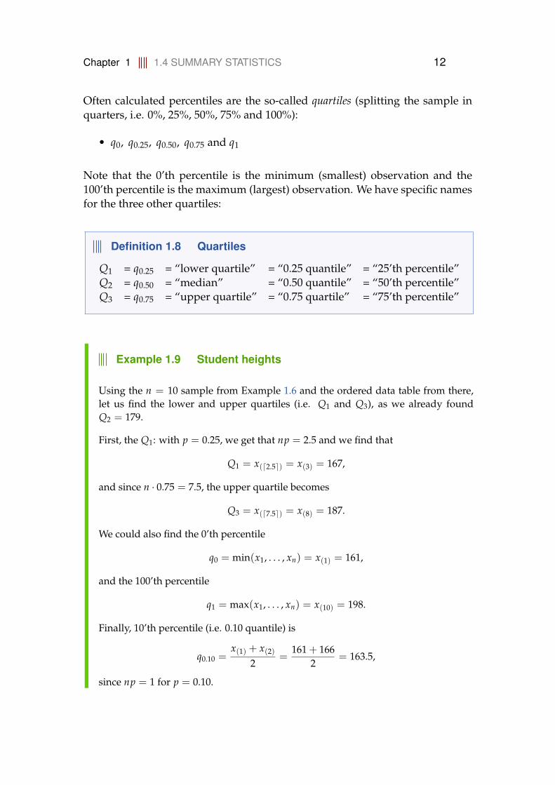
Definition 1.7 Quantiles and percentiles
The p quantile also called the 100p% quantile or 100p’th percentile, can bedefined by the following procedure: a
1. Order the n observations from smallest to largest: x(1), . . . , x(n)
2. Compute pn
3. If pn is an integer: average the pn’th and (pn + 1)’th ordered observa-tions. Then the p quantile is
qp =(
x(np) + x(np+1)
)/2 (1-4)
4. If pn is a noninteger: take the “next one” in the ordered list. Then thep’th quantile is
qp = x(dnpe), (1-5)
where dnpe is the ceiling of np, that is, the smallest integer larger thannp
aThere exist several other formal definitions. To obtain this definition of quan-tiles/percentiles in R use quantile(. . . , type=2). Using the default in R is also a perfectlyvalid approach - just a different one.
Chapter 1 1.4 SUMMARY STATISTICS 12
Often calculated percentiles are the so-called quartiles (splitting the sample inquarters, i.e. 0%, 25%, 50%, 75% and 100%):
• q0, q0.25, q0.50, q0.75 and q1
Note that the 0’th percentile is the minimum (smallest) observation and the100’th percentile is the maximum (largest) observation. We have specific namesfor the three other quartiles:
Definition 1.8 Quartiles
Q1 = q0.25 = “lower quartile” = “0.25 quantile” = “25’th percentile”Q2 = q0.50 = “median” = “0.50 quantile” = “50’th percentile”Q3 = q0.75 = “upper quartile” = “0.75 quartile” = “75’th percentile”
Example 1.9 Student heights
Using the n = 10 sample from Example 1.6 and the ordered data table from there,let us find the lower and upper quartiles (i.e. Q1 and Q3), as we already foundQ2 = 179.
First, the Q1: with p = 0.25, we get that np = 2.5 and we find that
Q1 = x(d2.5e) = x(3) = 167,
and since n · 0.75 = 7.5, the upper quartile becomes
Q3 = x(d7.5e) = x(8) = 187.
We could also find the 0’th percentile
q0 = min(x1, . . . , xn) = x(1) = 161,
and the 100’th percentile
q1 = max(x1, . . . , xn) = x(10) = 198.
Finally, 10’th percentile (i.e. 0.10 quantile) is
q0.10 =x(1) + x(2)
2=
161 + 1662
= 163.5,
since np = 1 for p = 0.10.
Chapter 1 1.4 SUMMARY STATISTICS 13
1.4.2 Measures of variability
A crucial aspect to understand when dealing with statistics is the concept ofvariability - the obvious fact that not everyone in a population, nor in a sample,will be exactly the same. If that was the case they would all equal the meanof the population or sample. But different phenomena will have different de-grees of variation: An adult (non dwarf) height population will maybe spreadfrom around 150 cm up to around 210 cm with very few exceptions. A kitchenscale measurement error population might span from −5 g to +5 g. We need away to quantify the degree of variability in a population and in a sample. Themost commonly used measure of sample variability is the sample variance orits square root, called the sample standard deviation:
Definition 1.10 Sample variance
The sample variance of a sample x1, . . . , xn is the sum of squared differencesfrom the sample mean divided by n− 1
s2 =1
n− 1
n
∑i=1
(xi − x)2. (1-6)
Definition 1.11 Sample standard deviation
The sample standard deviation is the square root of the sample variance
s =√
s2 =
√1
n− 1
n
∑i=1
(xi − x)2. (1-7)
The sample standard deviation and the sample variance are key numbers ofabsolute variation. If it is of interest to compare variation between differentsamples, it might be a good idea to use a relative measure - most obvious is thecoefficient of variation:
Chapter 1 1.4 SUMMARY STATISTICS 14
Definition 1.12 Coefficient of variation
The coefficient of variation is the sample standard deviation seen relative tothe sample mean
V =sx
. (1-8)
We interpret the standard deviation as the average absolute deviation from the meanor simply: the average level of differences, and this is by far the most used measureof spread. Two (relevant) questions are often asked at this point (it is perfectlyfine if you didn’t wonder about them by now and you might skip the answersand return to them later):
Remark 1.13
Question: Why not actually compute directly what the interpretation isstating, which would be: 1
n ∑ni=1 |xi − x|?
Answer: This is indeed an alternative, called the mean absolute deviation, thatone could use. The reason for most often measuring “mean deviation”NOT by the Mean Absolute Deviation statistic, but rather by the samplestandard deviation s, is the so-called theoretical statistical properties ofthe sample variance s2. This is a bit early in the material for going intodetails about this, but in short: inferential statistics is heavily basedon probability considerations, and it turns out that it is theoreticallymuch easier to put probabilities related to the sample variance s2 onexplicit mathematical formulas than probabilities related to most otheralternative measures of variability. Further, in many cases this choiceis in fact also the optimal choice in many ways.
Chapter 1 1.4 SUMMARY STATISTICS 15
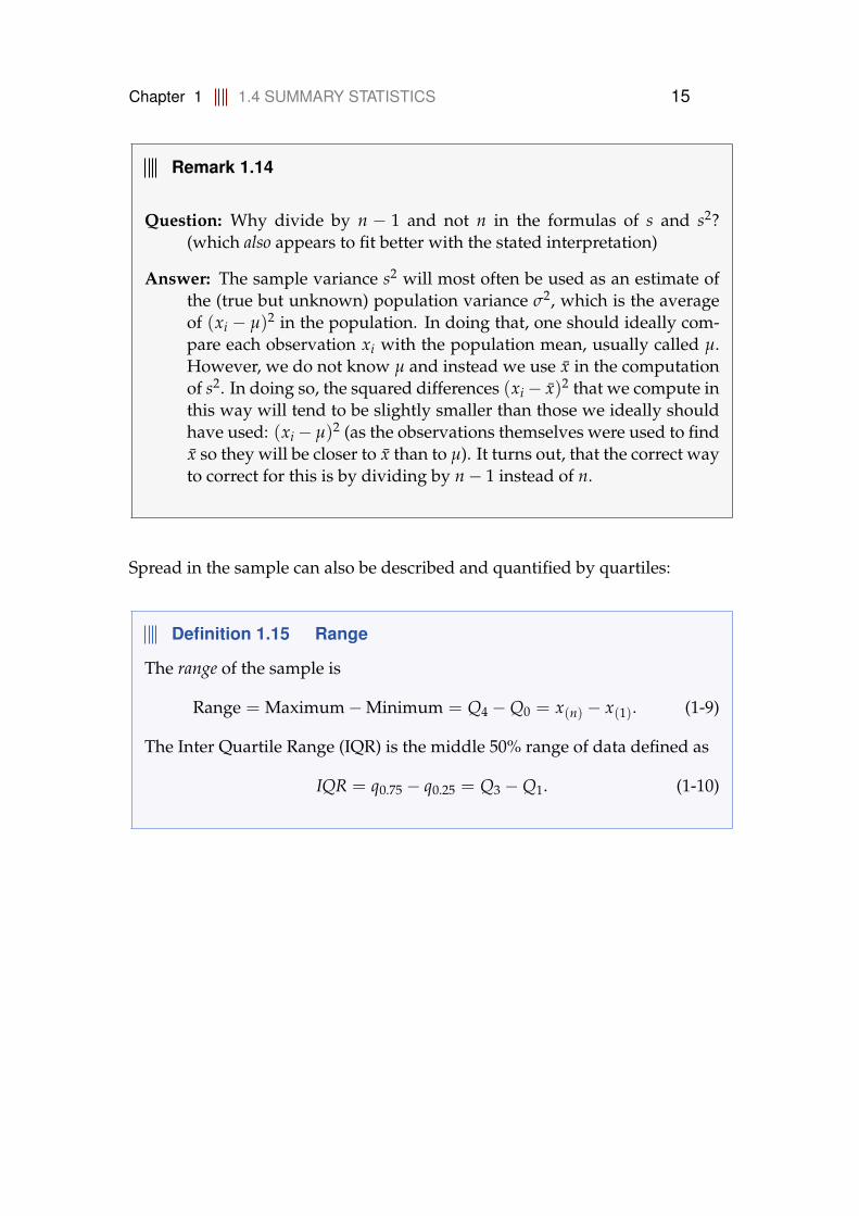
Remark 1.14
Question: Why divide by n − 1 and not n in the formulas of s and s2?(which also appears to fit better with the stated interpretation)
Answer: The sample variance s2 will most often be used as an estimate ofthe (true but unknown) population variance σ2, which is the averageof (xi − µ)2 in the population. In doing that, one should ideally com-pare each observation xi with the population mean, usually called µ.However, we do not know µ and instead we use x in the computationof s2. In doing so, the squared differences (xi− x)2 that we compute inthis way will tend to be slightly smaller than those we ideally shouldhave used: (xi− µ)2 (as the observations themselves were used to findx so they will be closer to x than to µ). It turns out, that the correct wayto correct for this is by dividing by n− 1 instead of n.
Spread in the sample can also be described and quantified by quartiles:
Definition 1.15 Range
The range of the sample is
Range = Maximum−Minimum = Q4 −Q0 = x(n) − x(1). (1-9)
The Inter Quartile Range (IQR) is the middle 50% range of data defined as
IQR = q0.75 − q0.25 = Q3 −Q1. (1-10)
Chapter 1 1.4 SUMMARY STATISTICS 16
Example 1.16 Student heights
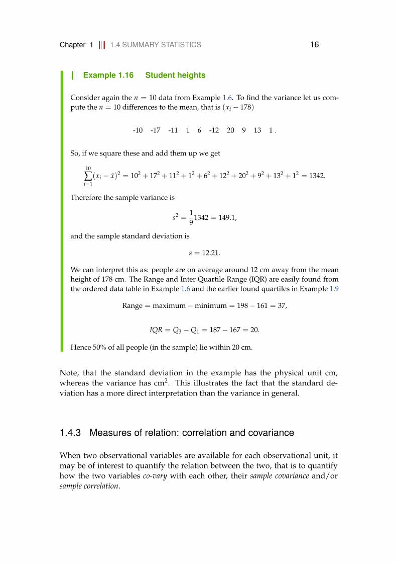
Consider again the n = 10 data from Example 1.6. To find the variance let us com-pute the n = 10 differences to the mean, that is (xi − 178)
-10 -17 -11 1 6 -12 20 9 13 1 .
So, if we square these and add them up we get
10
∑i=1
(xi − x)2 = 102 + 172 + 112 + 12 + 62 + 122 + 202 + 92 + 132 + 12 = 1342.
Therefore the sample variance is
s2 =19
1342 = 149.1,
and the sample standard deviation is
s = 12.21.
We can interpret this as: people are on average around 12 cm away from the meanheight of 178 cm. The Range and Inter Quartile Range (IQR) are easily found fromthe ordered data table in Example 1.6 and the earlier found quartiles in Example 1.9
Range = maximum−minimum = 198− 161 = 37,
IQR = Q3 −Q1 = 187− 167 = 20.
Hence 50% of all people (in the sample) lie within 20 cm.
Note, that the standard deviation in the example has the physical unit cm,whereas the variance has cm2. This illustrates the fact that the standard de-viation has a more direct interpretation than the variance in general.
1.4.3 Measures of relation: correlation and covariance
When two observational variables are available for each observational unit, itmay be of interest to quantify the relation between the two, that is to quantifyhow the two variables co-vary with each other, their sample covariance and/orsample correlation.

Chapter 1 1.4 SUMMARY STATISTICS 17
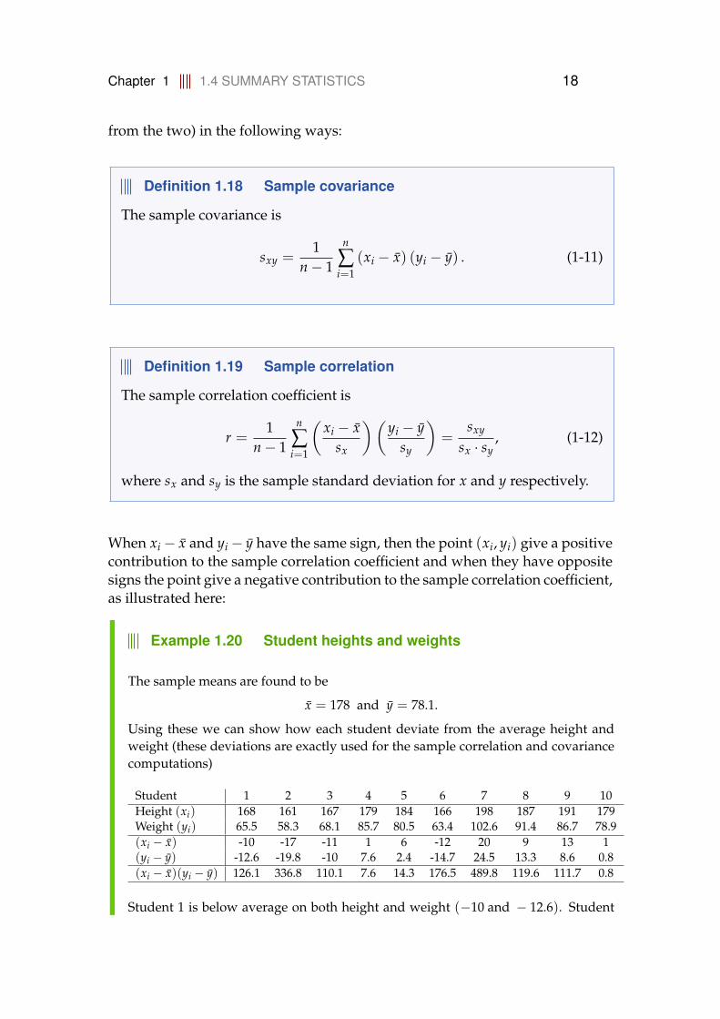
Example 1.17 Student heights and weights
In addition to the previously given student heights we also have their weights (inkg) available
Heights (xi) 168 161 167 179 184 166 198 187 191 179Weights (yi) 65.5 58.3 68.1 85.7 80.5 63.4 102.6 91.4 86.7 78.9
.
The relation between weights and heights can be illustrated by the so-called scatter-plot, cf. Section 1.6.4, where e.g. weights are plotted versus heights:
160 170 180 190
6070
8090
100
Height
Wei
ght
1
2
3
45
6
7
89
10
x = 178
y = 78.1
Each point in the plot corresponds to one student - here illustrated by using theobservation number as plot symbol. The (expected) relation is pretty clear now -different wordings could be used for what we see:
• Weights and heights are related to each other
• Higher students tend to weigh more than smaller students
• There is an increasing pattern from left to right in the "point cloud”
• If the point cloud is seen as an (approximate) ellipse, then the ellipse clearly ishorizontally upwards ”tilted”.
• Weights and heights are (positively) correlated to each other
The sample covariance and sample correlation coefficients are a summary statis-tics that can be calculated for two (related) sets of observations. They quantifythe (linear) strength of the relation between the two. They are calculated bycombining the two sets of observations (and the means and standard deviations
Chapter 1 1.4 SUMMARY STATISTICS 18
from the two) in the following ways:
Definition 1.18 Sample covariance
The sample covariance is
sxy =1
n− 1
n
∑i=1
(xi − x) (yi − y) . (1-11)
Definition 1.19 Sample correlation
The sample correlation coefficient is
r =1
n− 1
n
∑i=1
(xi − x
sx
)(yi − y
sy
)=
sxy
sx · sy, (1-12)
where sx and sy is the sample standard deviation for x and y respectively.
When xi− x and yi− y have the same sign, then the point (xi, yi) give a positivecontribution to the sample correlation coefficient and when they have oppositesigns the point give a negative contribution to the sample correlation coefficient,as illustrated here:
Example 1.20 Student heights and weights
The sample means are found to be
x = 178 and y = 78.1.
Using these we can show how each student deviate from the average height andweight (these deviations are exactly used for the sample correlation and covariancecomputations)
Student 1 2 3 4 5 6 7 8 9 10Height (xi) 168 161 167 179 184 166 198 187 191 179Weight (yi) 65.5 58.3 68.1 85.7 80.5 63.4 102.6 91.4 86.7 78.9(xi − x) -10 -17 -11 1 6 -12 20 9 13 1(yi − y) -12.6 -19.8 -10 7.6 2.4 -14.7 24.5 13.3 8.6 0.8(xi − x)(yi − y) 126.1 336.8 110.1 7.6 14.3 176.5 489.8 119.6 111.7 0.8
Student 1 is below average on both height and weight (−10 and − 12.6). Student

Chapter 1 1.4 SUMMARY STATISTICS 19
10 is above average on both height and weight (+1 and + 0.8).s
The sample covariance is then given by the sum of the 10 numbers in the last row ofthe table
sxy =19(126.1 + 336.8 + 110.1 + 7.6 + 14.3 + 176.5 + 489.8 + 119.6 + 111.7 + 0.8)
=19· 1493.3
= 165.9
And the sample correlation is then found from this number and the standard devia-tions
sx = 12.21 and sy = 14.07.
(the details of the sy computation is not shown). Thus we get the sample correlationas
r =165.9
12.21 · 14.07= 0.97.
Note how all 10 contributions to the sample covariance are positive in the ex-ample case - in line with the fact that all observations are found in the firstand third quadrants of the scatter plot (where the quadrants are defined by thesample means of x and y). Observations in second and fourth quadrant wouldcontribute with negative numbers to the sum, hence such observations wouldbe from students with below average on one feature while above average on theother. Then it is clear that: had all students been like that, then the covarianceand the correlation would have been negative, in line with a negative (down-wards) trend in the relation.
We can state (without proofs) a number of properties of the sample correlationr:
Remark 1.21 Properties of the sample correlation, r
• r is always between −1 and 1: −1 ≤ r ≤ 1
• r measures the degree of linear relation between x and y
• r = ±1 if and only if all points in the scatterplot are exactly on a line
• r > 0 if and only if the general trend in the scatterplot is positive
• r < 0 if and only if the general trend in the scatterplot is negative

Chapter 1 1.5 INTRODUCTION TO R AND RSTUDIO 20
The sample correlation coefficient measures the degree of linear relation be-tween x and y, which imply that we might fail to detect non-linear relationships,illustrated in the following plot of four different point clouds and their samplecorrelations:
0.0 0.2 0.4 0.6 0.8 1.0
0.0
0.4
0.8
1.2
r ≈ 0.95
x
y
0.0 0.2 0.4 0.6 0.8 1.0-2
-10
1
r ≈ −0.5
x
y
0.0 0.2 0.4 0.6 0.8 1.0
-3-2
-10
12
r ≈ 0
x
y
0.0 0.2 0.4 0.6 0.8 1.0
0.0
0.4
0.8
r ≈ 0
x
y
The sample correlation in both the bottom plots are close to zero, but as we seefrom the plot this number itself doesn’t imply that there no relation between yand x - which clearly is the case in the bottom right and highly non-linear case.
Sample covariances and correlation are closely related to the topic of linear re-gression, treated in Chapter 5 and 6 , where we will treat in more detail how wecan find the line that could be added to such scatterplots to describe the relationbetween x and y in a different (but related) way, as well as the statistical analysisused for this.
1.5 Introduction to R and RStudio
The program R is an open source software for statistics that you can downloadto your own laptop for free. Go to http://mirrors.dotsrc.org/cran/ and se-

Chapter 1 1.5 INTRODUCTION TO R AND RSTUDIO 21
lect your platform (Windows, Mac or Linux) and follow instructions to install.
RStudio is a free and open source integrated development environment (IDE)for R. You can run it on your desktop (Windows, Mac or Linux) or even overthe web using RStudio Server. It works as (an extended) alternative to running Rin the basic way through a terminal. This will be used in the course. Downloadit from http://www.rstudio.com/ and follow installation instructions. To usethe software, you only need to open RStudio (R will then be used by RStudio forcarrying out the calculations).
1.5.1 Console and scripts
Once you have opened RStudio, you will see a number of different windows.One of them is the console. Here you can write commands and execute them byhitting Enter. For instance:
> ## Add two numbers in the console> 2+3
[1] 5
In the console you cannot go back and change previous com-mands and neither can you save your work for later. To do thisyou need to write a script. Go to File->New->R Script. In thescript you can write a line and execute it in the console by hittingCtrl+Enter (Windows) or Cmd+Enter (Mac). You can also markseveral lines and execute them all at the same time.
1.5.2 Assignments and vectors
If you want to assign a value to a variable, you can use = or <-. The latter is thepreferred by R-users, so for instance:
> ## Assign the value 3 to y> y <- 3
It is often useful to assign a set of values to a variable like a vector. This is donewith the function c (short for concatenate):

Chapter 1 1.5 INTRODUCTION TO R AND RSTUDIO 22
## Concatenate numbers to a vectorx <- c(1, 4, 6, 2)x
[1] 1 4 6 2
Use the colon :, if you need a sequence, e.g. 1 to 10:
> ## A sequence from 1 to 10> x <- 1:10> x
[1] 1 2 3 4 5 6 7 8 9 10
You can also make a sequence with a specific stepsize different from 1
> ## Sequence with specified steps> x <- seq(0, 1, by=0.1)> x
[1] 0.0 0.1 0.2 0.3 0.4 0.5 0.6 0.7 0.8 0.9 1.0
If you are in doubt of how to use a certain function, the help page can be openedby typing ? followed by the function, e.g. ?seq.
If you know Matlab then this document Hiebeler-matlabR.pdf canbe very helpful.
1.5.3 Descriptive statistics
All the summary statistics measures presented in Section 1.4 can be found asfunctions or part of functions in R:
• mean(x) - mean value of the vector x
• var(x) - variance
• sd(x) - standard deviation
• median(x) - median

Chapter 1 1.5 INTRODUCTION TO R AND RSTUDIO 23
• quantile(x,p) - finds the pth quantile. p can consist of several differentvalues, e.g. quantile(x,c(0.25,0.75)) or quantile(x,c(0.25,0.75), type=2)
• cov(x, y) - the covariance of the vectors x and y
• cor(x, y) - the correlation
Please again note that the words quantiles and percentiles are used interchange-ably - they are essentially synonyms meaning exactly the same, even though theformal distinction has been clarified earlier.
Example 1.22 Summary statistics in R
Consider again the n = 10 data from Example 1.6. We can read these data into Rand compute the sample mean and sample median as follows:
## Sample Mean and Medianx <- c(168, 161, 167, 179, 184, 166, 198, 187, 191, 179)mean(x)
[1] 178
median(x)
[1] 179
The sample variance and sample standard deviation are found as follows:
## Sample variance and standard deviationvar(x)
[1] 149.1
sqrt(var(x))
[1] 12.21
sd(x)
[1] 12.21
The sample quartiles can be found by using the quantile function as follows:
Chapter 1 1.5 INTRODUCTION TO R AND RSTUDIO 24
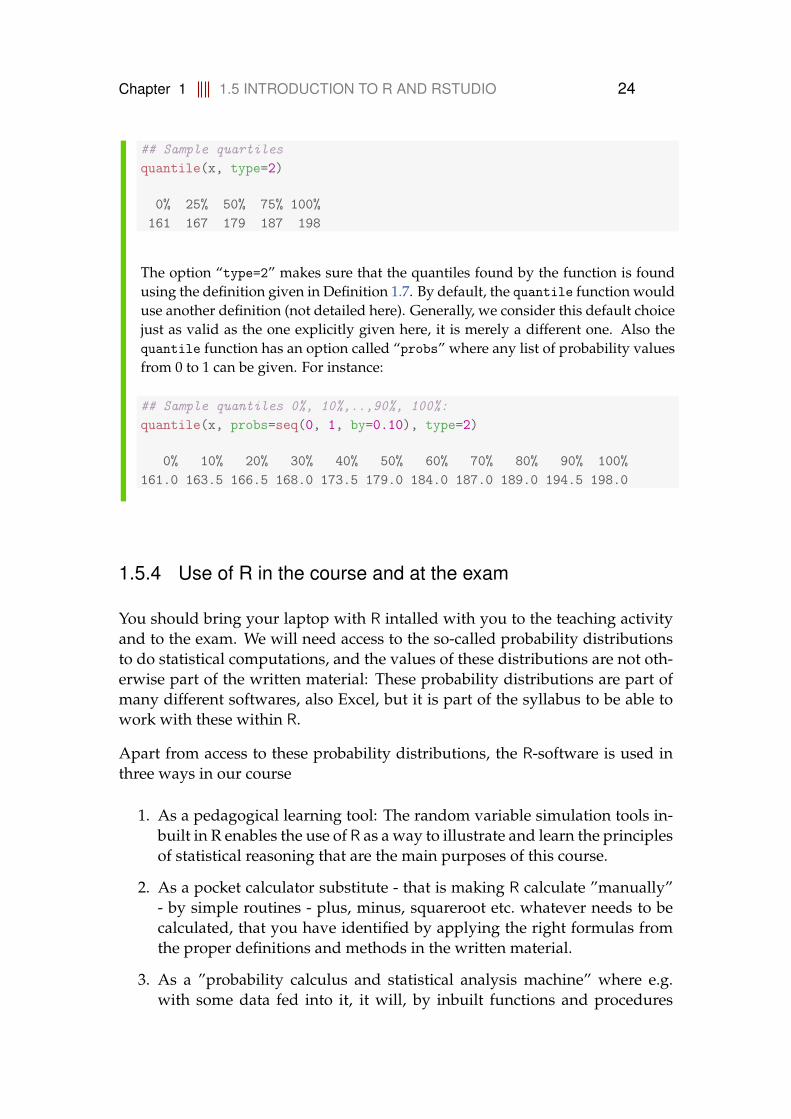
## Sample quartilesquantile(x, type=2)
0% 25% 50% 75% 100%161 167 179 187 198
The option “type=2” makes sure that the quantiles found by the function is foundusing the definition given in Definition 1.7. By default, the quantile function woulduse another definition (not detailed here). Generally, we consider this default choicejust as valid as the one explicitly given here, it is merely a different one. Also thequantile function has an option called “probs” where any list of probability valuesfrom 0 to 1 can be given. For instance:
## Sample quantiles 0%, 10%,..,90%, 100%:quantile(x, probs=seq(0, 1, by=0.10), type=2)
0% 10% 20% 30% 40% 50% 60% 70% 80% 90% 100%161.0 163.5 166.5 168.0 173.5 179.0 184.0 187.0 189.0 194.5 198.0
1.5.4 Use of R in the course and at the exam
You should bring your laptop with R intalled with you to the teaching activityand to the exam. We will need access to the so-called probability distributionsto do statistical computations, and the values of these distributions are not oth-erwise part of the written material: These probability distributions are part ofmany different softwares, also Excel, but it is part of the syllabus to be able towork with these within R.
Apart from access to these probability distributions, the R-software is used inthree ways in our course
1. As a pedagogical learning tool: The random variable simulation tools in-built in R enables the use of R as a way to illustrate and learn the principlesof statistical reasoning that are the main purposes of this course.
2. As a pocket calculator substitute - that is making R calculate ”manually”- by simple routines - plus, minus, squareroot etc. whatever needs to becalculated, that you have identified by applying the right formulas fromthe proper definitions and methods in the written material.
3. As a ”probability calculus and statistical analysis machine” where e.g.with some data fed into it, it will, by inbuilt functions and procedures
Chapter 1 1.5 INTRODUCTION TO R AND RSTUDIO 25
do all relevant computations for you and present the final results in someoverview tables and plots.
We will see and present all three types of applications of R during the course.For the first type, the aim is not to learn how to use the given R-code itselfbut rather to learn from the insights that the code together with the results ofapplying it is providing. It will be stated clearly whenever an R-example is ofthis type. Types 2 and 3 are specific tools that should be learned as a part of thecourse and represent tools that are explicitly relevant in your future engineeringactivity. It is clear that at some point one would love to just do the last kindof applications. However, it must be stressed that even though the program isable to calculate things for the user, understanding the details of the calculationsmust NOT be forgotten - understanding the methods and knowing the formulasis an important part of the syllabus, and will be checked at the exam.
Remark 1.23 BRING and USE pen and paper PRIOR to R
For many of the exercises that you are asked to do it will not be possible tojust directly identify what R-command(s) should be used to find the results.The exercises are often to be seen as what could be termed “problem math-ematics” exercises. So, it is recommended to also bring and use pen andpaper to work with the exercises to be able to subsequently know how tofinally finish them by some R-calculations.(If you adjusted yourself to somedigitial version of ”pen-and-paper”, then this is fine of course.)
Remark 1.24 R is not a substitute for your brain activity in thiscourse!
The software R should be seen as the most fantastic and easy computa-tional companion that we can have for doing statistical computations thatwe could have done ”manually”, if we wanted to spend the time doingit. All definitions, formulas, methods, theorems etc. in the written mate-rial should be known by the student, as should also certain R-routines andfunctions.
A good question to ask yourself each time that you apply en inbuilt R-functionis: ”Would I know how to make this computation ”manually”?”. There are fewexceptions to this requirement in the course, but only a few. And for these thequestion would be: ”Do I really understand what R is computing for me now?”

Chapter 1 1.6 PLOTTING, GRAPHICS - DATA VISUALISATION 26
1.6 Plotting, graphics - data visualisation
A really important part of working with data analysis is the visualisation of theraw data, as well as the results of the statistical analysis – the combination ofthe two leads to reliable results. Let us focus on the first part now, which canbe seen as being part of the explorative descriptive analysis also mentioned inSection 1.4. Depending on the data at hand different types of plots and graphicscould be relevant. One can distinguish between quantitative vs. categorical data.We will touch on the following type of basic plots:
• Quantitative data:
– Frequency plots and histograms
– box plots
– cumulative distribution
– Scatter plot (xy plot)
• Categorical data:
– Bar charts
– Pie charts
1.6.1 Frequency distributions and the histogram
The frequency distribution is the count of occurrences of values in the samplefor different classes using some classification, for example in intervals or bysome other property. It is nicely depicted by the histogram, which is a bar-plotof the occurrences in each classes.

Chapter 1 1.6 PLOTTING, GRAPHICS - DATA VISUALISATION 27
Example 1.25 Histogram in R
Consider again the n = 10 sample from Example 1.6.
## A histogram of the heightshist(x)
x
Freq
uenc
y
160 170 180 190 200
01
23
4
The default histogram uses equidistant interval widths (the same width for allintervals) and depicts the raw frequencies/counts in each interval. One maychange the scale into showing what we will learn to be densities by dividing theraw counts by n and the interval width, i.e.
"Interval count"n · ("Interval width")
.
By plotting the densities a density histogram also called the empirical densitythe area of all the bars add up to 1:
Chapter 1 1.6 PLOTTING, GRAPHICS - DATA VISUALISATION 28
Example 1.26 Empirical density in R
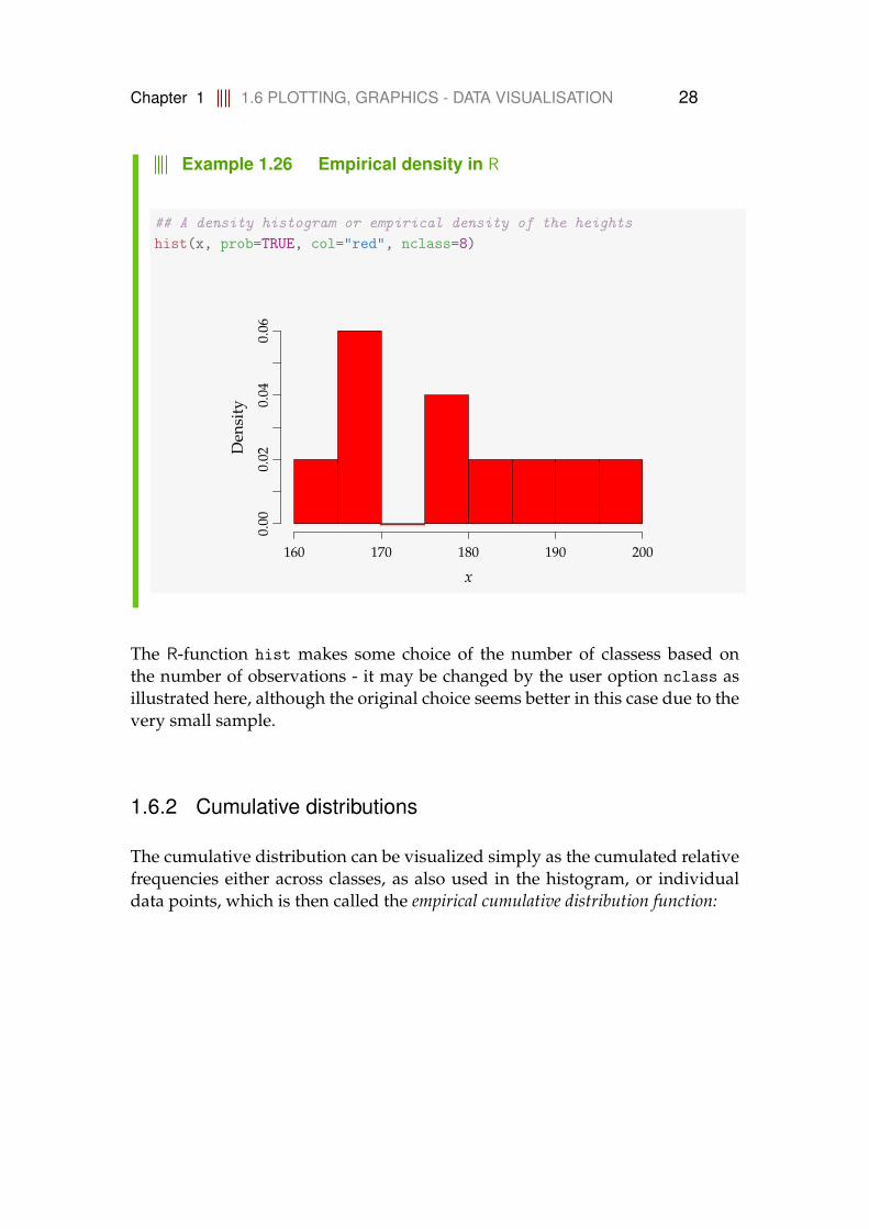
## A density histogram or empirical density of the heightshist(x, prob=TRUE, col="red", nclass=8)
x
Den
sity
160 170 180 190 200
0.00
0.02
0.04
0.06
The R-function hist makes some choice of the number of classess based onthe number of observations - it may be changed by the user option nclass asillustrated here, although the original choice seems better in this case due to thevery small sample.
1.6.2 Cumulative distributions
The cumulative distribution can be visualized simply as the cumulated relativefrequencies either across classes, as also used in the histogram, or individualdata points, which is then called the empirical cumulative distribution function:

Chapter 1 1.6 PLOTTING, GRAPHICS - DATA VISUALISATION 29
Example 1.27 Cumulative distribution plot in R
## Empirical cumulative distribution plotplot(ecdf(x), verticals=TRUE)
160 170 180 190 200
0.0
0.2
0.4
0.6
0.8
1.0
x
F(x)
The empirical cumulative distribution function Fn is a step function with jumpsi/n at observation values, where i is the number of identical(tied) observationsat that value.
For observations (x1, x2, . . . , xn), Fn(x) is the fraction of observations less orequal to x, that mathematically can be expressed as
Fn(x) = ∑j where xj≤x
1n
. (1-13)
1.6.3 The box plot and the modified box plot
The so-called box plot in its basic form depicts the five quartiles (min, Q1, me-dian, Q3, max) with a box from Q1 to Q3 emphasizing the Inter Quartile Range(IQR):

Chapter 1 1.6 PLOTTING, GRAPHICS - DATA VISUALISATION 30
Example 1.28 Box plot in R
## A basic box plot of the heights (range=0 makes it "basic")boxplot(x, range=0, col="red", main="Basic box plot")## Add the blue texttext(1.3, quantile(x), c("Minimum","Q1","Median","Q3","Maximum"),
col="blue")
160
170
180
190
Basic box plot
Minimum
Q1
Median
Q3
Maximum
In the modified box plot the whiskers only extend to the min. and max. obser-vation if they are not too far away from the box: defined to be 1.5× IQR. Obser-vations further away are considered as extreme observations and will be plottedindividually - hence the whiskers extend from the smallest to the largest obser-vation within a distance of 1.5× IQR of the box (defined as either 1.5× IQRlarger than Q3 or 1.5× IQR smaller than Q1).
Chapter 1 1.6 PLOTTING, GRAPHICS - DATA VISUALISATION 31
Example 1.29 Box plot in R
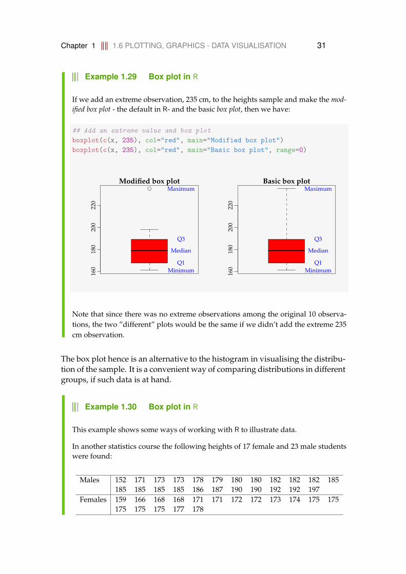
If we add an extreme observation, 235 cm, to the heights sample and make the mod-ified box plot - the default in R- and the basic box plot, then we have:
## Add an extreme value and box plotboxplot(c(x, 235), col="red", main="Modified box plot")boxplot(c(x, 235), col="red", main="Basic box plot", range=0)
160
180
200
220
Modified box plot
MinimumQ1
Median
Q3
Maximum
160
180
200
220
Basic box plot
MinimumQ1
Median
Q3
Maximum
Note that since there was no extreme observations among the original 10 observa-tions, the two ”different” plots would be the same if we didn’t add the extreme 235cm observation.
The box plot hence is an alternative to the histogram in visualising the distribu-tion of the sample. It is a convenient way of comparing distributions in differentgroups, if such data is at hand.
Example 1.30 Box plot in R
This example shows some ways of working with R to illustrate data.
In another statistics course the following heights of 17 female and 23 male studentswere found:
Males 152 171 173 173 178 179 180 180 182 182 182 185185 185 185 185 186 187 190 190 192 192 197
Females 159 166 168 168 171 171 172 172 173 174 175 175175 175 175 177 178
Chapter 1 1.6 PLOTTING, GRAPHICS - DATA VISUALISATION 32
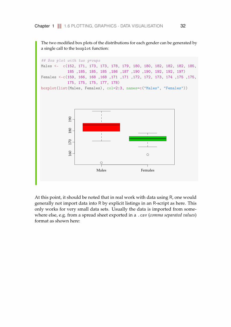
The two modified box plots of the distributions for each gender can be generated bya single call to the boxplot function:
## Box plot with two groupsMales <- c(152, 171, 173, 173, 178, 179, 180, 180, 182, 182, 182, 185,
185 ,185, 185, 185 ,186 ,187 ,190 ,190, 192, 192, 197)Females <-c(159, 166, 168 ,168 ,171 ,171 ,172, 172, 173, 174 ,175 ,175,
175, 175, 175, 177, 178)boxplot(list(Males, Females), col=2:3, names=c("Males", "Females"))
Males Females
160
170
180
190
At this point, it should be noted that in real work with data using R, one wouldgenerally not import data into R by explicit listings in an R-script as here. Thisonly works for very small data sets. Usually the data is imported from some-where else, e.g. from a spread sheet exported in a .csv (comma separated values)format as shown here:

Chapter 1 1.6 PLOTTING, GRAPHICS - DATA VISUALISATION 33
Example 1.31 Read and explore data in R
The gender grouped student heights data used in Example 1.30 is avail-able as a .csv-file via http://www2.compute.dtu.dk/courses/introstat/data/studentheights.csv. The structure of the data file, as it would appear in a spreadsheet program (e.g. LibreOffice Calc or Excel) is two columns and 40+1 rows includ-ing a header row:
1 Height Gender2 152 male3 171 male4 173 male. . .. . .24 197 male25 159 female26 166 female27 168 female. . .. . .39 175 female40 177 female41 178 female
The data can now be imported into R with the read.table function:
## Read the data (note that per default sep="," but here semicolon)studentheights <- read.table("studentheights.csv", sep=";", dec=".",
header=TRUE)
The resulting object studentheights is now a so-called data.frame, which is theclass used for such tables in R. There are some ways of getting a quick look at whatkind of data is really in a data set:

Chapter 1 1.6 PLOTTING, GRAPHICS - DATA VISUALISATION 34
## Have a look at the first 6 rows of the datahead(studentheights)
Height Gender1 152 male2 171 male3 173 male4 173 male5 178 male6 179 male
## Get an overviewstr(studentheights)
'data.frame': 40 obs. of 2 variables:$ Height: int 152 171 173 173 178 179 180 180 182 182 ...$ Gender: Factor w/ 2 levels "female","male": 2 2 2 2 2 2 2 2 2 2 ...
## Get a summary of each column/variable in the datasummary(studentheights)
Height GenderMin. :152.0 female:171st Qu.:172.8 male :23Median :177.5Mean :177.93rd Qu.:185.0Max. :197.0
For quantitative variables we get the quartiles and the mean from summary. Forcategorical variables we see (some of) the category frequencies . A data structure likethis is commonly encountered (and often the only needed) for statistical analysis.The gender grouped box plot can now be generated by:

Chapter 1 1.6 PLOTTING, GRAPHICS - DATA VISUALISATION 35
## Box plot for each genderboxplot(Height ~ Gender, data=studentheights, col=2:3)
female male
160
170
180
190
The R-syntax Height ~ Gender with the tilde symbol “~” is one that we will use alot in various contexts such as plotting and model fitting. In this context it can beunderstood as “Height is plotted as a function of Gender”.
1.6.4 The Scatter plot
The scatter plot can be used for two quantitative variables. It is simply onevariable plotted versus the other using some plotting symbol.
Example 1.32 Explore data included in R
Now we will use a data set available as part of R itself. Both base R and many addonR-packages include data sets, which can be used for testing and practicing. Here wewill use the mtcars data set. If you write:
## See information about the mtcars data?mtcars
you will be able to read the following as part of the help info:
“The data was extracted from the 1974 Motor Trend US magazine, and comprises fuel con-sumption and 10 aspects of automobile design and performance for 32 automobiles (1973-74
Chapter 1 1.6 PLOTTING, GRAPHICS - DATA VISUALISATION 36
models). A data frame with 32 observations on 11 variables. Source: Henderson and Velle-man (1981), Building multiple regression models interactively. Biometrics, 37, 391-411.”
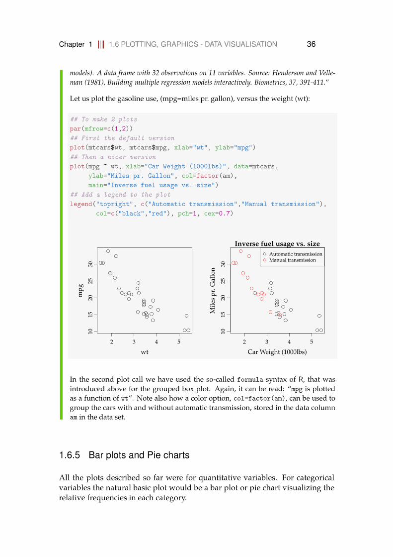
Let us plot the gasoline use, (mpg=miles pr. gallon), versus the weight (wt):
## To make 2 plotspar(mfrow=c(1,2))## First the default versionplot(mtcars$wt, mtcars$mpg, xlab="wt", ylab="mpg")## Then a nicer versionplot(mpg ~ wt, xlab="Car Weight (1000lbs)", data=mtcars,
ylab="Miles pr. Gallon", col=factor(am),main="Inverse fuel usage vs. size")
## Add a legend to the plotlegend("topright", c("Automatic transmission","Manual transmission"),
col=c("black","red"), pch=1, cex=0.7)
2 3 4 5
1015
2025
30
wt
mpg
2 3 4 5
1015
2025
30
Inverse fuel usage vs. size
Car Weight (1000lbs)
Mile
spr
.Gal
lon
Automatic transmissionManual transmission
In the second plot call we have used the so-called formula syntax of R, that wasintroduced above for the grouped box plot. Again, it can be read: “mpg is plottedas a function of wt”. Note also how a color option, col=factor(am), can be used togroup the cars with and without automatic transmission, stored in the data columnam in the data set.
1.6.5 Bar plots and Pie charts
All the plots described so far were for quantitative variables. For categoricalvariables the natural basic plot would be a bar plot or pie chart visualizing therelative frequencies in each category.

Chapter 1 1.6 PLOTTING, GRAPHICS - DATA VISUALISATION 37
Example 1.33 Bar plots and Pie charts in R
For the gender grouped student heights data used in Example 1.30 we can plot thegender distribution by:
## Barplotbarplot(table(studentheights$Gender), col=2:3)
female male
05
1015
20
## Pie chartpie(table(studentheights$Gender), cex=1, radius=1)
female
male

Chapter 1 1.6 PLOTTING, GRAPHICS - DATA VISUALISATION 38
1.6.6 More plots in R?
A good place for getting more inspired on how to do easy and nice plots in R is:http://www.statmethods.net/.

Chapter 1 1.7 EXERCISES 39
1.7 Exercises
Exercise 1.1 Infant birth weight
In a study of different occupational groups the infant birth weight was recordedfor randomly selected babies born by hairdressers, who had their first child.The following table shows the weight in grams (observations specified in sortedorder) for 10 female births and 10 male births:
Females (x) 2474 2547 2830 3219 3429 3448 3677 3872 4001 4116Males (y) 2844 2863 2963 3239 3379 3449 3582 3926 4151 4356
Solve at least the following questions a)-c) first “manually” and then by theinbuilt functions in R. It is OK to use R as alternative to your pocket calculatorfor the “manual” part, but avoid the inbuilt functions that will produce theresults without forcing you to think about how to compute it during the manualpart.
a) What is the sample mean, variance and standard deviation of the femalebirths? Express in your own words the story told by these numbers. Theidea is to force you to interpret what can be learned from these numbers.
b) Compute the same summary statistics of the male births. Compare andexplain differences with the results for the female births.
c) Find the five quartiles for each sample — and draw the two box plots withpen and paper (i.e. not using R.)
d) Are there any “extreme” observations in the two samples (use the modifiedbox plot definition of extremness)?
e) What are the coefficient of variations in the two groups?

Chapter 1 1.7 EXERCISES 40
Exercise 1.2 Course grades
To compare the difficulty of 2 different courses at a university the followinggrades distributions (given as number of pupils who achieved the grades) wereregistered:
Course 1 Course 2 TotalGrade 12 20 14 34Grade 10 14 14 28Grade 7 16 27 43Grade 4 20 22 42Grade 2 12 27 39Grade 0 16 17 33Grade -3 10 22 32Total 108 143 251
a) What is the median of the 251 achieved grades?
b) What are the quartiles and the IQR (Inter Quartile Range)?
Exercise 1.3 Cholesterol
In a clinical trial of a cholesterol-lowering agent, 15 patients’ cholesterol (inmmol L−1) was measured before treatment and 3 weeks after starting treatment.Data is listed in the following table:
Patient 1 2 3 4 5 6 7 8 9 10 11 12 13 14 15Before 9.1 8.0 7.7 10.0 9.6 7.9 9.0 7.1 8.3 9.6 8.2 9.2 7.3 8.5 9.5After 8.2 6.4 6.6 8.5 8.0 5.8 7.8 7.2 6.7 9.8 7.1 7.7 6.0 6.6 8.4
a) What is the median of the cholesterol measurements for the patients beforetreatment, and similarly after treatment?
b) Find the standard deviations of the cholesterol measurements of the pa-tients before and after treatment.

Chapter 1 1.7 EXERCISES 41
c) Find the sample covariance between cholesterol measurements of the pa-tients before and after treatment.
d) Find the sample correlation between cholesterol measurements of the pa-tients before and after treatment.
e) Compute the 15 differences (Dif = Before − After) and do various sum-mary statistics and plotting of these: sample mean, sample variance, sam-ple standard deviation, boxplot etc.
f) Observing such data the big question is whether an average decrease incholesterol level can be “shown statistically”. How to formally answerthis question is presented in Chapter 3, but consider now which summarystatistics and/or plots would you look at to have some idea of what theanswer will be?
Exercise 1.4 Project start
a) Go to CampusNet and take a look at the first project and read the projectpage on the website for more information (02323.compute.dtu.dk/Agendasor 02402.compute.dtu.dk/Agendas). Follow the steps to import the datainto R and get started with the explorative data analysis.
Chapter 2 42
Chapter 2
Probability and simulation
In this chapter elements from probability theory are introduced. These areneeded to form the basic mathematical description of randomness. For examplefor calculating the probabilities of outcomes in various types of experimental orobservational study setups. Small illustrative examples, such as e.g. dice rollsand lottery draws, and natural phenomena such as the waiting time betweenradioactive decays are used as throughout. But the scope of probability theoryand it’s use in society, science and business, not least engineering endavour,goes way beyond these small examples. The theory is introduced together withillustrative R code examples, which the reader is encouraged to try and interactwith in parallel to reading the text. Many of these are of the learning type, cf.the discussion of the way R is used in the course in Section 1.5.
2.1 Random variable
The basic building blocks to describe random outcomes of an experiment areintroduced in this section. The definition of an experiment is quite broad. It canbe an experiment, which is carried out under controlled conditions e.g. in alaboratory or flipping a coin, as well as an experiment in conditions which arenot controlled, where for example a process is observed e.g. observations ofthe GNP or measurements taken with a space telescope. Hence, an experimentcan be thought of as any setting in which the outcome cannot be fully known.This for example also includes measurement noise, which are random “errors”related to the system used to observe with, maybe originating from noise inelectrical circuits or small turbulence around the sensor. Measurements willalways contain some noise.
First the sample space is defined:

Chapter 2 2.1 RANDOM VARIABLE 43
Definition 2.1
The sample space S is the set of all possible outcomes of an experiment.
Example 2.2
Consider an experiment in which a person will throw two paper balls with the pur-pose of hitting a wastebasket. All the possible outcomes forms the sample space ofthis experiment as
S ={(miss,miss), (hit,miss), (miss,hit), (hit,hit)
}. (2-1)
Now a random variable can be defined:
Definition 2.3
A random variable is a function which assigns a numerical value to each out-come in the sample space. In this book random variables are denoted withcapital letters, e.g.
X, Y, . . . . (2-2)
Example 2.4
Continuing the paper ball example above, a random variable can be defined as thenumber of hits, thus
X((miss,miss)
)= 0, (2-3)
X((hit,miss)
)= 1, (2-4)
X((miss,hit)
)= 1, (2-5)
X((hit,hit)
)= 2. (2-6)
In this case the random variable is a function which maps the sample space S topositive integers, i.e. X : S→N0.

Chapter 2 2.1 RANDOM VARIABLE 44
Remark 2.5
The random variable represents a value of the outcome before the experimentis carried out. Usually the experiment is carried out n times and there arerandom variables for each of them
{Xi : 1, 2, . . . , n}. (2-7)
After the experiment has been carried out n times a set of values of the ran-dom variable is available as
{xi : 1, 2, . . . , n}. (2-8)
Each value is called a realization or observation of the random variable andis denoted with a small letter sub-scripted with an index i, as introduced inChapter 1.
Finally, in order to quantify probability, a random variable is associated witha probability distribution. The distribution can either be discrete or continuousdepending on the nature of the outcomes:
• Discrete outcomes can for example be: the outcome of a dice roll, the num-ber of children per family, or the number of failures of a machine per year.Hence some countable phenomena which can be represented by an inte-ger.
• Continuous outcomes can for example by: the weight of the yearly har-vest, the time spend on homework each week, or the electricity generationper hour. Hence a phenomena which can be represented by a continuousvalue.
Furthermore, the outcome can either be unlimited or limited. This is most ob-vious in the case discrete case, e.g. a dice roll is limited to the values between1 and 6. However it is also often the case for continuous random variables, forexample many are non-negative (weights, distances, etc.) and proportions arelimited to a range between 0 and 1.
Conceptually there is no difference between the discrete and the continuouscase, however it is easier to distinguish since the formulas, which in the discretecase are with sums, in the continuous case are with integrals. In the remainingof this chapter, first the discrete case is presented and then the continuous.

Chapter 2 2.2 DISCRETE RANDOM VARIABLES 45
2.2 Discrete random variables
In this section discrete distributions and their properties are introduced. A dis-crete random variable has discrete outcomes and follows a discrete distribution.
To exemplify, consider the outcome of one roll of a fair six-sided dice as therandom variable Xfair. It has six possible outcomes, each with equal probability.This is specified with the probability density function.
Definition 2.6
For a discrete random variable X the probability density function (pdf) is
f (x) = P(X = x). (2-9)
It assigns a probability to every possible outcome value x.A discrete pdf fulfills two properties: there are no negative probabilities forany outcome value
f (x) ≥ 0 for all x, (2-10)
and the probabilities for all outcome values sum to one
∑all x
f (x) = 1. (2-11)
Example 2.7
For the fair dice the pdf is
x 1 2 3 4 5 6fXfair(x) 1
616
16
16
16
16
If the dice is not fair, maybe it has been modified to increase the probability of rollinga six, the pdf could for example be
x 1 2 3 4 5 6fXunfair(x) 1
717
17
17
17
27
where Xunfair is a random variable representing the value of a roll with the unfairdice.
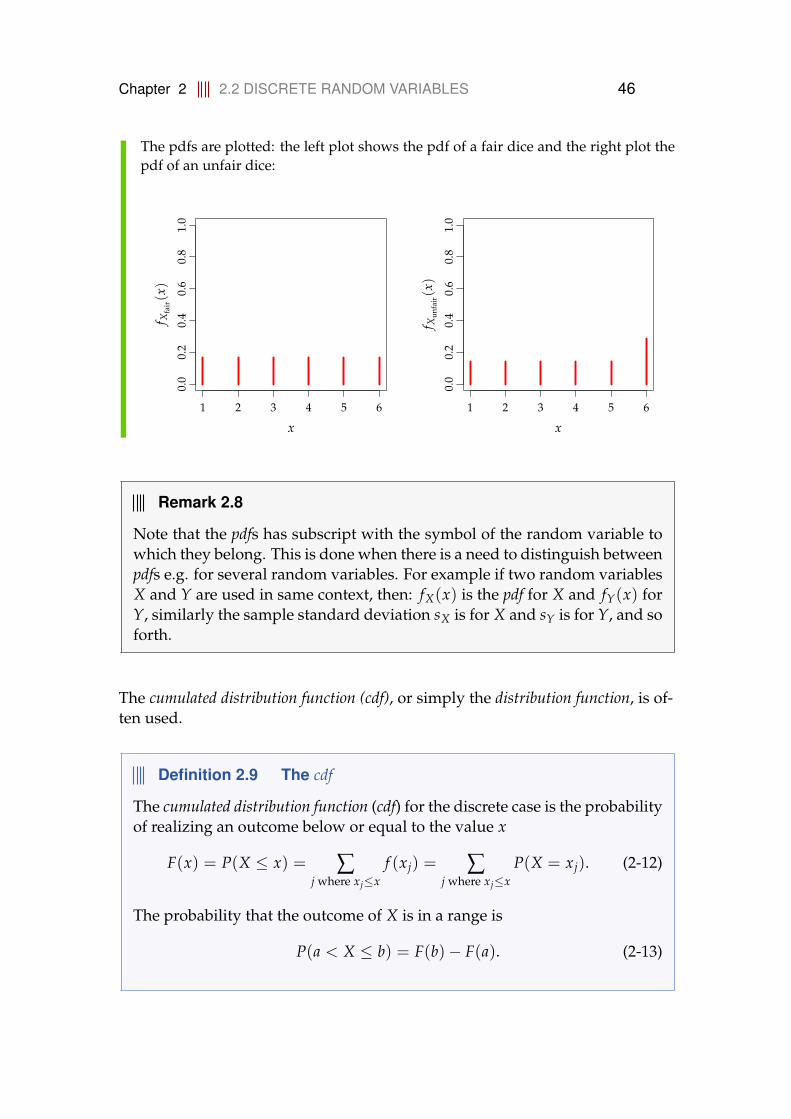
Chapter 2 2.2 DISCRETE RANDOM VARIABLES 46
The pdfs are plotted: the left plot shows the pdf of a fair dice and the right plot thepdf of an unfair dice:
1 2 3 4 5 6
0.0
0.2
0.4
0.6
0.8
1.0
x
f Xfa
ir(x)
1 2 3 4 5 6
0.0
0.2
0.4
0.6
0.8
1.0
xf X
unfa
ir(x)
Remark 2.8
Note that the pdfs has subscript with the symbol of the random variable towhich they belong. This is done when there is a need to distinguish betweenpdfs e.g. for several random variables. For example if two random variablesX and Y are used in same context, then: fX(x) is the pdf for X and fY(x) forY, similarly the sample standard deviation sX is for X and sY is for Y, and soforth.
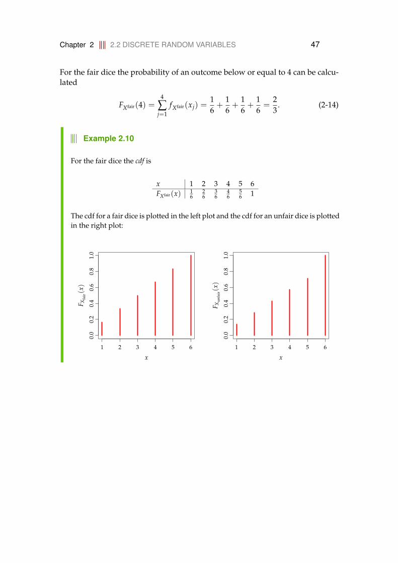
The cumulated distribution function (cdf), or simply the distribution function, is of-ten used.
Definition 2.9 The cdf
The cumulated distribution function (cdf) for the discrete case is the probabilityof realizing an outcome below or equal to the value x
F(x) = P(X ≤ x) = ∑j where xj≤x
f (xj) = ∑j where xj≤x
P(X = xj). (2-12)
The probability that the outcome of X is in a range is
P(a < X ≤ b) = F(b)− F(a). (2-13)
Chapter 2 2.2 DISCRETE RANDOM VARIABLES 47
For the fair dice the probability of an outcome below or equal to 4 can be calcu-lated
FXfair(4) =4
∑j=1
fXfair(xj) =16+
16+
16+
16=
23
. (2-14)
Example 2.10
For the fair dice the cdf is
x 1 2 3 4 5 6FXfair(x) 1
626
36
46
56 1
The cdf for a fair dice is plotted in the left plot and the cdf for an unfair dice is plottedin the right plot:
1 2 3 4 5 6
0.0
0.2
0.4
0.6
0.8
1.0
x
F Xfa
ir(x)
1 2 3 4 5 6
0.0
0.2
0.4
0.6
0.8
1.0
x
F Xun
fair(x)
Chapter 2 2.2 DISCRETE RANDOM VARIABLES 48
2.2.1 Introduction to simulation
One nice thing about having computers available is that we try things in virtualreality - this we can here use here to play around while learning how prob-ability and statistics work. With the pdf defined an experiment can easily besimulated, i.e. instead of carrying out the experiment in reality it is carried outusing a model on the computer. When the simulation includes generating ran-dom numbers it is called a stochastic simulation. Such simulation tools are readilyavailable within R, and it can be used for as well learning purposes as a way todo large scale complex probabilistic and statistical computations. For now itwill be used in the first way.
Example 2.11 Simulation of rolling a dice
Let’s simulate the experiment of rolling a dice using the following R code (open thefile chapter2-ProbabilitySimulation.R and try it)
## Make a random draw from (1,2,3,4,5,6) with equal probability## for each outcomesample(1:6, size=1)
The simulation becomes more interesting when the experiment is repeated manytimes, then we have a sample and can calculate the empirical density function (or em-pirical pdf or density histogram, see Section 1.6.1) as a discrete histogram and actually“see” the shape of the pdf
## Simulate a fair dice
## Number of simulated realizationsn <- 30## Draw independently from the set (1,2,3,4,5,6) with equal probabilityxFair <- sample(1:6, size=n, replace=TRUE)## Count the number of each outcome using the table functiontable(xFair)## Plot the pdfpar(mfrow=c(1,2))plot(rep(1/6,6), type="h", col="red", ylim=c(0,1), lwd=10)## Plot the empirical pdflines(table(xFair)/n, lwd=4)## Plot the cdfplot(cumsum(rep(1/6,6)), ylim=c(0,1), lwd=10, type="h", col="red")## Add the empirical cdflines(cumsum(table(xFair)/n), lwd=4, type="h")

Chapter 2 2.2 DISCRETE RANDOM VARIABLES 49
1 2 3 4 5 6
0.0
0.2
0.4
0.6
0.8
1.0
x
Den
sity
pdfEmpirical pdf
1 2 3 4 5 6
0.0
0.2
0.4
0.6
0.8
1.0
x
Cum
ulat
edde
nsit
yTry simulating with different number of rolls n and describe how this affectsthe accuracy of the empirical pdf compared to the pdf?
Now repeat this with the unfair dice
## Simulate an unfair dice
## Number of simulated realizationsn <- 30## Draw independently from the set (1,2,3,4,5,6) with higher## probability for a sixxUnfair <- sample(1:6, size=n, replace=TRUE, prob=c(rep(1/7,5),2/7))## Plot the pdfplot(c(rep(1/7,5),2/7), type="h", col="red", ylim=c(0,1), lwd=10)## Plot the empirical density functionlines(table(xUnfair)/n, lwd=4)## Plot the cdfplot(cumsum(c(rep(1/7,5),2/7)), ylim=c(0,1), lwd=10, type="h", col="red")## Add the empirical cdflines(cumsum(table(xUnfair)/n), lwd=4, type="h")
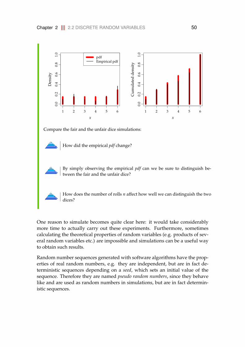
Chapter 2 2.2 DISCRETE RANDOM VARIABLES 50
1 2 3 4 5 6
0.0
0.2
0.4
0.6
0.8
1.0
x
Den
sity
pdfEmpirical pdf
1 2 3 4 5 6
0.0
0.2
0.4
0.6
0.8
1.0
x
Cum
ulat
edde
nsit
yCompare the fair and the unfair dice simulations:
How did the empirical pdf change?
By simply observing the empirical pdf can we be sure to distinguish be-tween the fair and the unfair dice?
How does the number of rolls n affect how well we can distinguish the twodices?
One reason to simulate becomes quite clear here: it would take considerablymore time to actually carry out these experiments. Furthermore, sometimescalculating the theoretical properties of random variables (e.g. products of sev-eral random variables etc.) are impossible and simulations can be a useful wayto obtain such results.
Random number sequences generated with software algorithms have the prop-erties of real random numbers, e.g. they are independent, but are in fact de-terministic sequences depending on a seed, which sets an initial value of thesequence. Therefore they are named pseudo random numbers, since they behavelike and are used as random numbers in simulations, but are in fact determin-istic sequences.

Chapter 2 2.2 DISCRETE RANDOM VARIABLES 51
Remark 2.12 Random numbers and seed in R
In R the initial values can be set with a single number called the seed asdemonstrated with the following R code. As default the seed is created fromthe time of start-up of a new instance of R. A way to generate truly (i.e. non-pseudo) random numbers can be to sample some physical phenomena, forexample atmospheric noise as done at www.random.org.
## The random numbers generated depends on the seed
## Set the seedset.seed(127)## Generate a (pseudo) random sequencesample(1:10)
[1] 3 1 2 8 7 4 10 9 6 5
## Generate again and see that new numbers are generatedsample(1:10)
[1] 9 3 7 2 10 8 6 1 5 4
## Set the seed and the same numbers as before just after the## seed was set are generatedset.seed(127)sample(1:10)
[1] 3 1 2 8 7 4 10 9 6 5
2.2.2 Mean and variance
In Chapter 1 the sample mean and the sample variance were introduced. Theyindicate respectively the centering and the spread of data, i.e. of a sample. Inthis section the mean and variance are introduced. They are properties of thedistribution of a random variable, they are called population parameters. Themean indicates where the distribution is centered. The variance indicates thespread of the distribution.

Chapter 2 2.2 DISCRETE RANDOM VARIABLES 52
Mean and expected value
The mean (µ) of a random variable is the population parameter which most sta-tistical analysis focus on. It is formally defined as a function E(X): the expectedvalue of the random variable X.
Definition 2.13 Mean value
The mean of a discrete random variable X is
µ = E(X) =∞
∑i=1
xi f (xi), (2-15)
where xi is the value and f (xi) is the probability that X takes the outcomevalue xi.
The mean is simply the weighted average over all possible outcome values,weighted with the corresponding probability. As indicated in the definitionthere might be infinitely many possible outcome values, hence, even if the totalsum of probabilities is one, then the probabilities must go sufficiently fast tozero for increasing values of X in order for the sum to be defined.
Example 2.14
For the fair dice the mean is calculated by
µxfair = E(Xfair) = 116+ 2
16+ 3
16+ 4
16+ 5
16+ 6
16= 3.5,
for the unfair dice the mean is
µxunfair = E(Xunfair) = 117+ 2
17+ 3
17+ 4
17+ 5
17+ 6
27≈ 3.86.
The mean of a random variable express the limiting value of an average of manyoutcomes. If a fair dice is rolled a really high number of times the sample meanof these will be very close to 3.5. For the statistical reasoning related to the use ofa sample mean as an estimate for µ, the same property ensures that envisioningmany sample means (with the same n), a meta like thinking, then the mean ofsuch many repeated sample means will be close to µ.
After an experiment has been carried out n times then the sample mean or average
Chapter 2 2.2 DISCRETE RANDOM VARIABLES 53
can be calculated as previously defined in Chapter 1
µ = x =1n
n
∑i
xi. (2-16)
It is called a statistic, which means that it is calculated from a sample. Note theuse of a hat in the notation over µ: this indicates that it is an estimate of the realunderlying mean.
Our intuition tells us that the estimate (µ) will be close to true underlying ex-pectation (µ) when n is large. This is indeed the case, to be more specificE[
1n ∑ Xi
]= µ (when E[Xi] = µ), and we say that the average is a central
estimator for the expectation. The exact quantification of these qualitative state-ments will be covered in Chapter 3.
Now play a little around with the mean and the sample mean with some simu-lations.
Example 2.15 Simulate and estimate the mean
Carrying out the experiment more than one time an estimate of the mean, i.e. thesample mean, can be calculated. Simulate rolling the fair dice
## Simulate a fair dice
## Number of realizationsn <- 30## Simulate rolls with a fair dicexFair <- sample(1:6, size=n, replace=TRUE)## Calculate the sample meansum(xFair)/n
[1] 3.6
## ormean(xFair)
[1] 3.6
Let us see what happens with the sample mean of the unfair dice by simulating thesame number of rolls
Chapter 2 2.2 DISCRETE RANDOM VARIABLES 54
## Simulate an unfair dice
## n realizationsxUnfair <- sample(1:6, size=n, replace=TRUE, prob=c(rep(1/7,5),2/7))## Calculate the sample meanmean(xUnfair)
[1] 3.967
Consider the mean of the unfair dice and compare it to the mean of the fairdice (see Example 2.14). Is this in accordance with your simulation results?
Let us again turn to how much we can “see” from the simulations and the impactof the number of realizations n on the estimation. In statistics the term information isused to refer to how much information is embedded in the data, and therefore howaccurate different properties (parameters) can be estimated from the data.
Repeat the simulations several times with n = 30. By simply comparing thesample means from a single simulation can it then be determined if the twomeans really are different?
Repeat the simulations several times and increase n. What happens with tothe ’accuracy’ of the sample mean compared to the real mean? and therebyhow well it can be inferred if the sample means are different?
Does the information embedded in the data increase or decrease when n isincreased?
Variance and standard deviation
The second most used population parameter is the variance (or standard devia-tion). It is a measure describing the spread of the distribution, more specificallythe spread away from the mean.

Chapter 2 2.2 DISCRETE RANDOM VARIABLES 55
Definition 2.16 Variance
The variance of a discrete random variable X is
σ2 = V(X) = E[(X− µ)2] =∞
∑i=1
(xi − µ)2 f (xi), (2-17)
where xi is the outcome value and f (xi) is the pdf of the ith outcome value.The standard deviation σ is the square root of the variance.
The variance is the expected value (i.e. average (weighted by probabilities)) ofthe squared distance between the outcome and the mean value.
Remark 2.17
Notice that the variance cannot be negative.
The standard deviation is measured on the same scale (same units) as the ran-dom variable, which is not case for the variance. Therefore the standard de-viation can much easier be interpreted, when communicating the spread of adistribution.
Consider how the expected value is calculated in Equation (2-15).One can think of the squared distance as a new random variablethat has an expected value which is the variance of X.
Example 2.18
The variance of rolls with the fair dice is
σ2xfair = E[(Xfair − µXfair)2]
= (1− 3.5)2 16+ (2− 3.5)2 1
6+ (3− 3.5)2 1
6+ (4− 3.5)2 1
6+ (5− 3.5)2 1
6+ (6− 3.5)2 1
6
=7024
≈ 2.92.
It was seen in Chapter 1, that after an experiment has been carried out n times
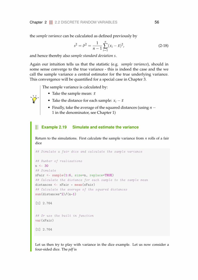
Chapter 2 2.2 DISCRETE RANDOM VARIABLES 56
the sample variance can be calculated as defined previously by
s2 = σ2 =1
n− 1
n
∑i=1
(xi − x)2, (2-18)
and hence thereby also sample standard deviation s.
Again our intuition tells us that the statistic (e.g. sample variance), should insome sense converge to the true variance - this is indeed the case and the wecall the sample variance a central estimator for the true underlying variance.This convergence will be quantified for a special case in Chapter 3.
The sample variance is calculated by:
• Take the sample mean: x
• Take the distance for each sample: xi − x
• Finally, take the average of the squared distances (using n−1 in the denominator, see Chapter 1)
Example 2.19 Simulate and estimate the variance
Return to the simulations. First calculate the sample variance from n rolls of a fairdice
## Simulate a fair dice and calculate the sample variance
## Number of realizationsn <- 30## SimulatexFair <- sample(1:6, size=n, replace=TRUE)## Calculate the distance for each sample to the sample meandistances <- xFair - mean(xFair)## Calculate the average of the squared distancessum(distances^2)/(n-1)
[1] 2.764
## Or use the built in functionvar(xFair)
[1] 2.764
Let us then try to play with variance in the dice example. Let us now consider afour-sided dice. The pdf is
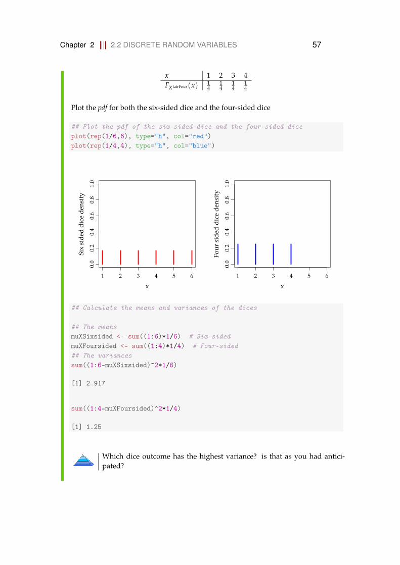
Chapter 2 2.2 DISCRETE RANDOM VARIABLES 57
x 1 2 3 4FXfairFour(x) 1
414
14
14
Plot the pdf for both the six-sided dice and the four-sided dice
## Plot the pdf of the six-sided dice and the four-sided diceplot(rep(1/6,6), type="h", col="red")plot(rep(1/4,4), type="h", col="blue")
1 2 3 4 5 6
0.0
0.2
0.4
0.6
0.8
1.0
x
Six
side
ddi
cede
nsit
y
1 2 3 4 5 6
0.0
0.2
0.4
0.6
0.8
1.0
x
Four
side
ddi
cede
nsit
y
## Calculate the means and variances of the dices
## The meansmuXSixsided <- sum((1:6)*1/6) # Six-sidedmuXFoursided <- sum((1:4)*1/4) # Four-sided## The variancessum((1:6-muXSixsided)^2*1/6)
[1] 2.917
sum((1:4-muXFoursided)^2*1/4)
[1] 1.25
Which dice outcome has the highest variance? is that as you had antici-pated?
Chapter 2 2.3 DISCRETE DISTRIBUTIONS 58
2.3 Discrete distributions
In this section the discrete distributions included in the material are presented.See the overview of all distributions in the collection of formulas Section A.2.1.
In R, implementations of many different distributions are available. For eachdistribution at least the following is available
• The pdf is available by preceding with 'd', e.g. for the binomial distribu-tion dbinom
• The cdf is available by preceding with 'p', e.g. pbinom
• The quantiles by preceding with 'q', e.g. qbinom
• Random number generation by preceding with 'r' e.g. rbinom
See for example the help with ?dbinom in R and see the names of all the R func-tions in the overview A.2.1. They are demonstrated below in this section for thediscrete and later for the continuous distributions, see them demonstrated forthe normal distribution in Example 2.45.
2.3.1 Binomial distribution
The binomial distribution is a very important discrete distribution and appearsin many applications, it is presented in this section. In statistics it is typicallyused for proportions as explained in Chapter 7.
If an experiment has two possible outcomes (e.g. failure or success, no or yes, 0or 1) and is repeated more than one time, then the number of successes may bebinomial distributed. For example the number of heads obtained after a certainnumber of flips with a coin. Each repetition must be independent. In relation torandom sampling this corresponds to successive draws with replacement (thinkof drawing notes from a hat, where after each draw the note is put back again,i.e. the drawn number is replaced again).

Chapter 2 2.3 DISCRETE DISTRIBUTIONS 59
Definition 2.20 Binomial distribution
Let the random variable X be binomial distributed
X ∼ B(n, p), (2-19)
where n is number of independent draws and p is the probability of a suc-cess in each draw.The binomial pdf describes probability of obtaining x successes
f (x; n, p) = P(X = x) =
(nx
)px(1− p)n−x, (2-20)
where(
nx
)=
n!x!(n− x)!
, (2-21)
is the number of distinct sets of x elements which can be chosen from a setof n elements. Remember that n! = n · (n− 1) · . . . · 2 · 1.
Theorem 2.21 Mean and variance
The mean of a binomial distributed random variable is
µ = np, (2-22)
and the variance is
σ2 = np(1− p). (2-23)
Actually this can be proved by calculating the mean using Definition 2.13 andthe variance using Definition 2.16.
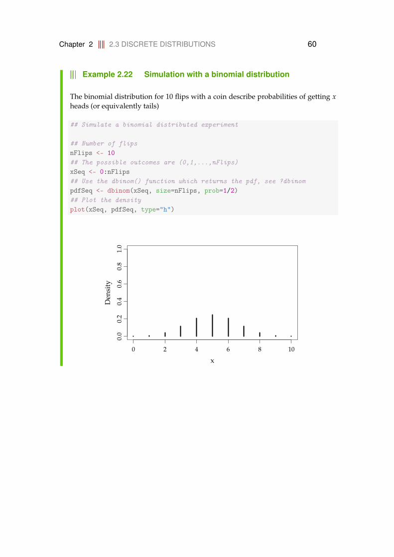
Chapter 2 2.3 DISCRETE DISTRIBUTIONS 60
Example 2.22 Simulation with a binomial distribution
The binomial distribution for 10 flips with a coin describe probabilities of getting xheads (or equivalently tails)
## Simulate a binomial distributed experiment
## Number of flipsnFlips <- 10## The possible outcomes are (0,1,...,nFlips)xSeq <- 0:nFlips## Use the dbinom() function which returns the pdf, see ?dbinompdfSeq <- dbinom(xSeq, size=nFlips, prob=1/2)## Plot the densityplot(xSeq, pdfSeq, type="h")
0 2 4 6 8 10
0.0
0.2
0.4
0.6
0.8
1.0
x
Den
sity
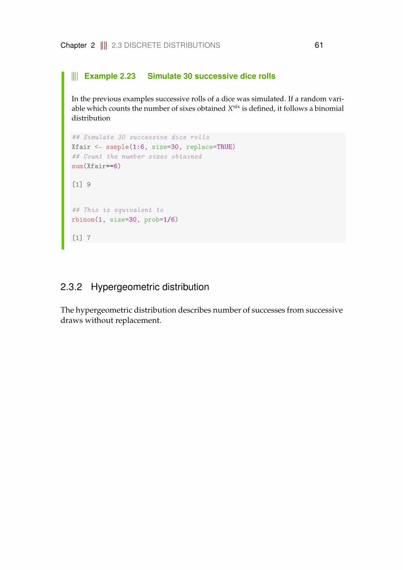
Chapter 2 2.3 DISCRETE DISTRIBUTIONS 61
Example 2.23 Simulate 30 successive dice rolls
In the previous examples successive rolls of a dice was simulated. If a random vari-able which counts the number of sixes obtained Xsix is defined, it follows a binomialdistribution
## Simulate 30 successive dice rollsXfair <- sample(1:6, size=30, replace=TRUE)## Count the number sixes obtainedsum(Xfair==6)
[1] 9
## This is equivalent torbinom(1, size=30, prob=1/6)
[1] 7
2.3.2 Hypergeometric distribution
The hypergeometric distribution describes number of successes from successivedraws without replacement.
Chapter 2 2.3 DISCRETE DISTRIBUTIONS 62
Definition 2.24 Hypergeometric distribution
Let the random variable X be the number of successes in n draws withoutreplacement. Then X follows the hypergeometric distribution
X ∼ H(n, a, N), (2-24)
where a is the number of successes in the N elements large population. Theprobability of obtaining x successes is described by the hypergeometric pdf
f (x; n, a, N) = P(X = x) =(a
x)(N−an−x)
(Nn )
. (2-25)
The notation(
ab
)=
a!b!(a− b)!
, (2-26)
represents the number of distinct sets of b elements which can be chosenfrom a set of a elements.
Theorem 2.25 Mean and variance
The mean of a hypergeometric distributed random variable is
µ = naN
, (2-27)
and the variance is
σ2 = na(N − a)
N2N − nN − 1
. (2-28)
Example 2.26 Lottery probabilities using the hypergeometric dis-tribution
A lottery drawing is a good example where the hypergeometric distribution can beapplied. The numbers from 1 to 90 are put in a bowl and randomly drawn withoutreplacement (i.e. without putting back the number when it has been drawn). Saythat you have the sheet with 8 numbers and want to calculate the probability ofgetting all 8 numbers in 25 draws.

Chapter 2 2.3 DISCRETE DISTRIBUTIONS 63
## The probability of getting x numbers of the sheet in 25 drawings
## Number of successes in the populationa <- 8## Size of the populationN <- 90## Number of drawsn <- 25## Plot the pdf, note: parameters names are different in the R functionplot(0:8, dhyper(x=0:8,m=a,n=N-a,k=n), type="h")
0 2 4 6 8
0.0
0.1
0.2
0.3
0.4
0.5
x
Den
sity
n = 25a = 8N = 90
2.3.3 Poisson distribution
The Poisson distribution describes the probability of a given number of eventsoccurring in a fixed interval if these events occur with a known average rateand independently of the distance to the last event. Often it is events in a timeinterval, but can as well be counts in other intervals, e.g. of distance, area orvolume. In statistics the Poisson distribution is usually applied for analyzingfor example counts of: arrivals, traffic, failures and breakdowns.

Chapter 2 2.3 DISCRETE DISTRIBUTIONS 64
Definition 2.27 Poisson distribution
Let the random variable X be Poisson distributed
X ∼ Po(λ), (2-29)
where λ is the rate (or intensity): the average number of events per interval.The Poisson pdf describes the probability of x events in an interval
f (x; λ) =λx
x!e−λ. (2-30)
Theorem 2.28 Mean and variance
A Poisson distributed random variable X has exactly the rate λ as the mean
µ = λ, (2-31)
and variance
σ2 = λ. (2-32)
Example 2.29
The Poisson distribution is typically used to describe phenomena such as:
• the number radioactive particle decays per time interval, i.e. the number ofclicks per time interval of a Geiger counter
• calls to a call center per time interval (λ does vary over the day)
• number of mutations in a given stretch of DNA after a certain amount of radi-ation
• goals scored in a soccer match
One important feature is that the rate can be scaled, such that probabilities ofoccurrences in other interval lengths can be calculated. Usually the rate is de-noted with the interval length, for example the hourly rate is denoted as λhour

Chapter 2 2.3 DISCRETE DISTRIBUTIONS 65
and can be scaled to the minutely rate by
λminute =λhour
60, (2-33)
such the probabilities of x events per minute can be calculated with the Poissonpdf with rate λminute.
Example 2.30 Rate scaling
You are enjoying a soccer match. Assuming that the scoring of goals per match inthe league is Poisson distributed and on average 3.4 goals are scored per match.Calculate the probability that no goals will be scored while you leave the match for10 minutes.
Let λ90minutes = 3.4 be goals per match and scale this to the 10 minute rate by
λ10minutes =λ90minutes
9=
3.49
. (2-34)
Let X be the number of goals in 10 minute intervals and use this to calculate theprobability of no events a 10 minute interval by
P(X = 0) = f (0, λ10minutes) ≈ 0.685, (2-35)
which was found with the R code
## Probability of no goals in 10 minutes
## The Poisson pdfdpois(x=0, lambda=3.4/9)
[1] 0.6854
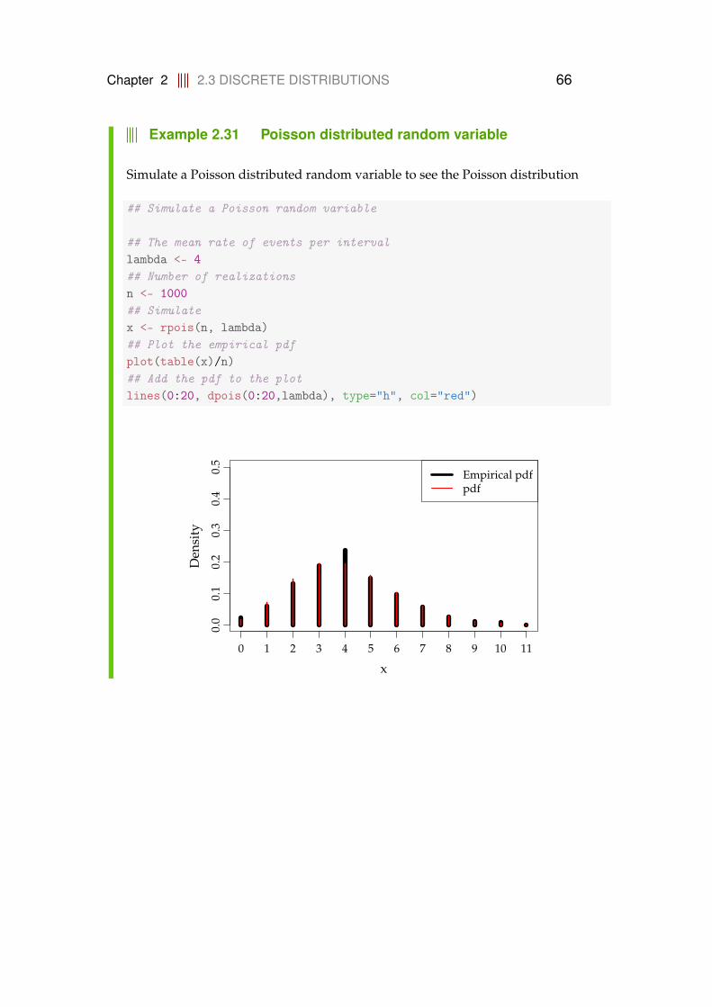
Chapter 2 2.3 DISCRETE DISTRIBUTIONS 66
Example 2.31 Poisson distributed random variable
Simulate a Poisson distributed random variable to see the Poisson distribution
## Simulate a Poisson random variable
## The mean rate of events per intervallambda <- 4## Number of realizationsn <- 1000## Simulatex <- rpois(n, lambda)## Plot the empirical pdfplot(table(x)/n)## Add the pdf to the plotlines(0:20, dpois(0:20,lambda), type="h", col="red")
0.0
0.1
0.2
0.3
0.4
0.5
x
Den
sity
0 1 2 3 4 5 6 7 8 9 10 11
Empirical pdfpdf
Chapter 2 2.4 CONTINUOUS RANDOM VARIABLES 67
2.4 Continuous random variables
If an outcome of an experiment takes a continuous value, for example: a dis-tance, a temperature, a weight, etc., then it is represented by a continuous ran-dom variable.
Definition 2.32 Density and probabilities
The pdf of a continuous random variable X is a non-negative function for allpossible outcomes
f (x) ≥ 0 for all x, (2-36)
and has an area below the function of one∫ ∞
−∞f (x)dx = 1. (2-37)
It defines the probability of observing an outcome in the range from a to bby
P(a < X ≤ b) =∫ b
af (x)dx. (2-38)
For the discrete case the probability of observing an outcome x is equal to thepdf of x, but this is not the case for a continuous random variable, where
P(X = x) = P(x < X ≤ x) =∫ x
xf (u)du = 0, (2-39)
i.e. the probability for a continuous random variable to be realized at a singlenumber P(X = x) is zero.
The plot in Figure 2.1 shows how the area below the pdf represents the proba-bility of observing an outcome in a range. Note that the normal distribution isused here for the examples, it is introduced in Section 2.5.2.
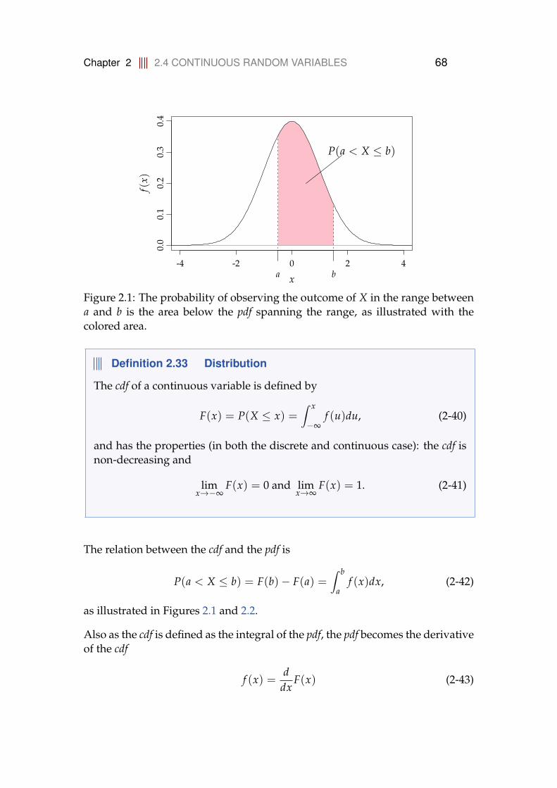
Chapter 2 2.4 CONTINUOUS RANDOM VARIABLES 68
-4 -2 0 2 4
0.0
0.1
0.2
0.3
0.4
x
f(x)
P(a < X ≤ b)
a b
Figure 2.1: The probability of observing the outcome of X in the range betweena and b is the area below the pdf spanning the range, as illustrated with thecolored area.
Definition 2.33 Distribution
The cdf of a continuous variable is defined by
F(x) = P(X ≤ x) =∫ x
−∞f (u)du, (2-40)
and has the properties (in both the discrete and continuous case): the cdf isnon-decreasing and
limx→−∞
F(x) = 0 and limx→∞
F(x) = 1. (2-41)
The relation between the cdf and the pdf is
P(a < X ≤ b) = F(b)− F(a) =∫ b
af (x)dx, (2-42)
as illustrated in Figures 2.1 and 2.2.
Also as the cdf is defined as the integral of the pdf, the pdf becomes the derivativeof the cdf
f (x) =d
dxF(x) (2-43)

Chapter 2 2.4 CONTINUOUS RANDOM VARIABLES 69
-4 -2 0 2 4
0.0
0.2
0.4
0.6
0.8
1.0
x
F(x)
P(a
<X
≤b)
=F(
b)−
F(a)
a b
Figure 2.2: The probability of observing the outcome of X in the range betweena and b is the distance between F(a) and F(b).
2.4.1 Mean and Variance
Definition 2.34 Mean and variance
For a continuous random variable the mean or expected value is
µ = E(X) =∫ ∞
−∞x f (x)dx, (2-44)
hence similar as for the discrete case the outcome is weighted with the pdf.The variance is
σ2 = E[(X− µ)2] =∫ ∞
−∞(x− µ)2 f (x)dx, (2-45)
The differences between the discrete and the continuous case can be summedup in two points:
• In the continuous case integrals are used, in the discrete case sums areused.
• In the continuous case the probability of observing a single value is alwayszero. In the discrete case it can be positive or zero.

Chapter 2 2.5 CONTINUOUS DISTRIBUTIONS 70
2.5 Continuous distributions
2.5.1 Uniform distribution
A random variable following the uniform distribution has equal density at anyvalue within a defined range.
Definition 2.35 Uniform distribution
Let X be a uniform distributed random variable
X ∼ U(α, β), (2-46)
where α and β defines the range of possible outcomes. It has the pdf
f (x) =
{1
β−α for x ∈ [α, β]
0 otherwise. (2-47)
The uniform cdf is
F(x) =
0 for x < αx−αβ−α for x ∈ [α, β)
1 for x ≥ β
. (2-48)
In Figure 2.3 the uniform pdf and cdf are plotted.
Theorem 2.36 Mean and variance of the uniform distribution
The mean of a uniform distributed random variable X is
µ =12(α + β), (2-49)
and the variance is
σ2 =1
12(β− α)2. (2-50)
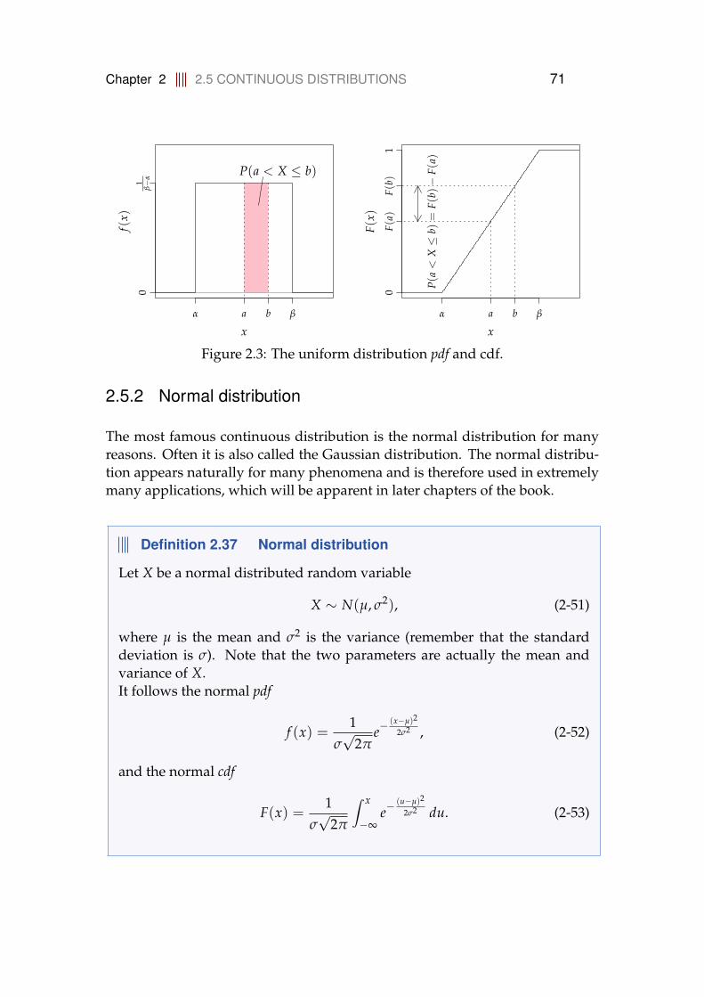
Chapter 2 2.5 CONTINUOUS DISTRIBUTIONS 71
x
f(x)
P(a < X ≤ b)
α a b β
01
β−
α
x
F(x)
P(a
<X
≤b)
=F(
b)−
F(a)
01
α a b β
F(a)
F(b)
Figure 2.3: The uniform distribution pdf and cdf.
2.5.2 Normal distribution
The most famous continuous distribution is the normal distribution for manyreasons. Often it is also called the Gaussian distribution. The normal distribu-tion appears naturally for many phenomena and is therefore used in extremelymany applications, which will be apparent in later chapters of the book.
Definition 2.37 Normal distribution
Let X be a normal distributed random variable
X ∼ N(µ, σ2), (2-51)
where µ is the mean and σ2 is the variance (remember that the standarddeviation is σ). Note that the two parameters are actually the mean andvariance of X.It follows the normal pdf
f (x) =1
σ√
2πe−
(x−µ)2
2σ2 , (2-52)
and the normal cdf
F(x) =1
σ√
2π
∫ x
−∞e−
(u−µ)2
2σ2 du. (2-53)

Chapter 2 2.5 CONTINUOUS DISTRIBUTIONS 72
Theorem 2.38 Mean and variance
The mean of a Normal distributed random variable is
µ, (2-54)
and the variance is
σ2. (2-55)
Hence simply the two parameters defining the distribution.
Example 2.39 The normal pdf
Example: Let us play with the normal pdf
## Play with the normal distribution
## The mean and standard deviationmuX <- 0sigmaX <- 1## A sequence of x valuesxSeq <- seq(-6, 6, by=0.1)##pdfX <- 1/(sigmaX*sqrt(2*pi)) * exp(-(xSeq-muX)^2/(2*sigmaX^2))## Plot the pdfplot(xSeq, pdfX, type="l", xlab="$x$", ylab="f(x)")
-6 -4 -2 0 2 4 6
0.0
0.1
0.2
0.3
0.4
x
f(x)
Chapter 2 2.5 CONTINUOUS DISTRIBUTIONS 73
Try with different values of the mean and standard deviation. Describe howthis change the position and spread of the pdf?
Theorem 2.40 Linear combinations of normal random variables
Let X1, . . . , Xn be independent normal random variables, then any linearcombination of X1, . . . , Xn will follow a normal distribution, with mean andvariance given in Theorem 2.56.
Use the mean and variance identities introduced in Section 2.7 to find the meanand variance of the linear combination as exemplified here:
Example 2.41
Consider two normal distributed random variables
X1 ∼ N(µX1 , σ2X1) and X2 ∼ N(µX2 , σ2
X2). (2-56)
The difference
Y = X1 − X2, (2-57)
is normal distributed
Y ∼ N(µY, σ2Y), (2-58)
where the mean is
µY = µX1 − µX2 , (2-59)
and
σ2Y = σ2
X1+ σ2
X2, (2-60)
where the mean and variance identities introduced in Section 2.7 have been used.
Standard normal distribution
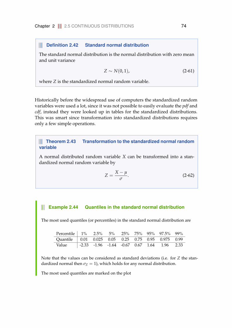
Chapter 2 2.5 CONTINUOUS DISTRIBUTIONS 74
Definition 2.42 Standard normal distribution
The standard normal distribution is the normal distribution with zero meanand unit variance
Z ∼ N(0, 1), (2-61)
where Z is the standardized normal random variable.
Historically before the widespread use of computers the standardized randomvariables were used a lot, since it was not possible to easily evaluate the pdf andcdf, instead they were looked up in tables for the standardized distributions.This was smart since transformation into standardized distributions requiresonly a few simple operations.
Theorem 2.43 Transformation to the standardized normal randomvariable
A normal distributed random variable X can be transformed into a stan-dardized normal random variable by
Z =X− µ
σ. (2-62)
Example 2.44 Quantiles in the standard normal distribution
The most used quantiles (or percentiles) in the standard normal distribution are
Percentile 1% 2.5% 5% 25% 75% 95% 97.5% 99%Quantile 0.01 0.025 0.05 0.25 0.75 0.95 0.975 0.99Value -2.33 -1.96 -1.64 -0.67 0.67 1.64 1.96 2.33
Note that the values can be considered as standard deviations (i.e. for Z the stan-dardized normal then σZ = 1), which holds for any normal distribution.
The most used quantiles are marked on the plot
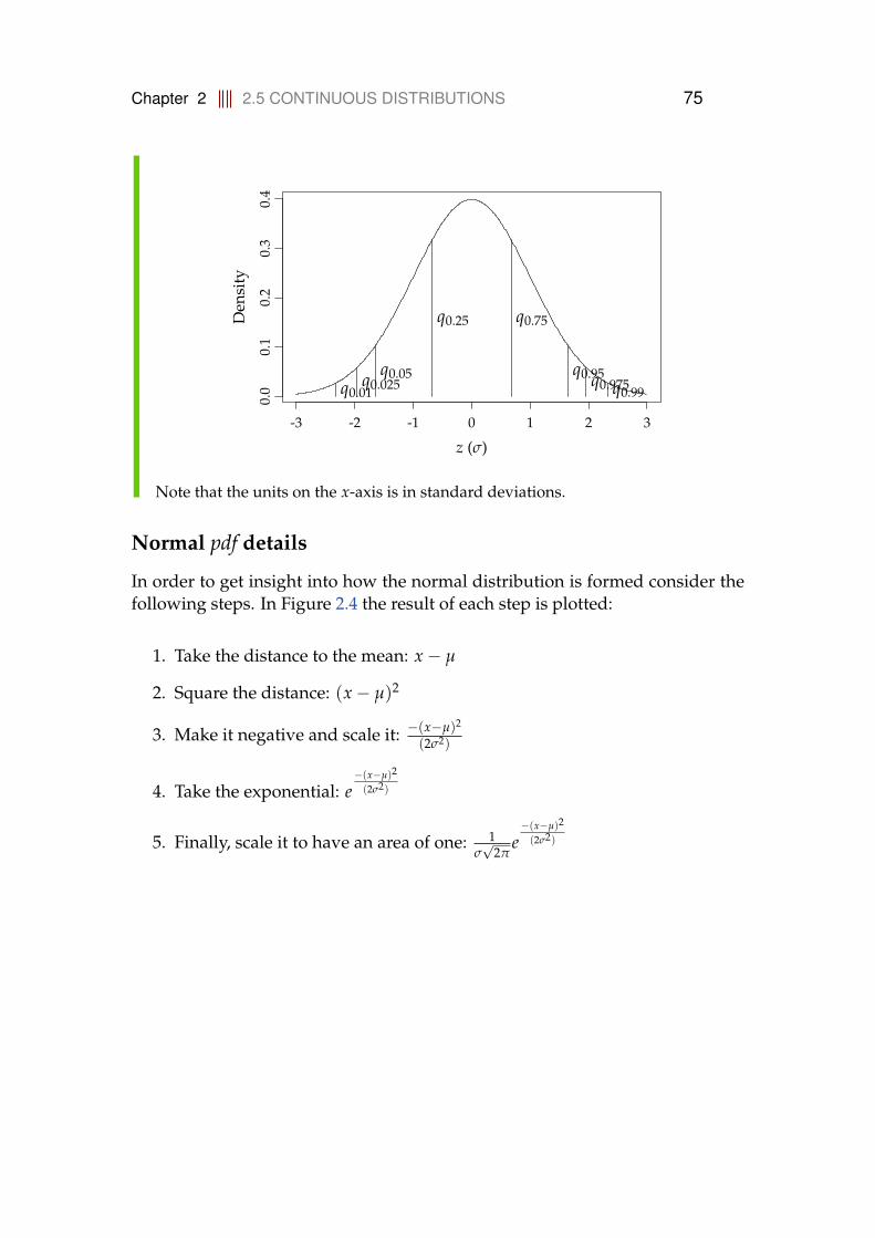
Chapter 2 2.5 CONTINUOUS DISTRIBUTIONS 75
-3 -2 -1 0 1 2 3
0.0
0.1
0.2
0.3
0.4
z (σ)
Den
sity
q0.01q0.025
q0.05
q0.25 q0.75
q0.95q0.975q0.99
Note that the units on the x-axis is in standard deviations.
Normal pdf details
In order to get insight into how the normal distribution is formed consider thefollowing steps. In Figure 2.4 the result of each step is plotted:
1. Take the distance to the mean: x− µ
2. Square the distance: (x− µ)2
3. Make it negative and scale it: −(x−µ)2
(2σ2)
4. Take the exponential: e−(x−µ)2
(2σ2)
5. Finally, scale it to have an area of one: 1σ√
2πe−(x−µ)2
(2σ2)
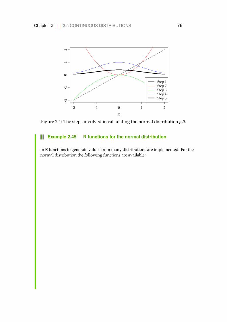
Chapter 2 2.5 CONTINUOUS DISTRIBUTIONS 76
-2 -1 0 1 2
-2-1
01
2
x
Step 1Step 2Step 3Step 4Step 5
Figure 2.4: The steps involved in calculating the normal distribution pdf.
Example 2.45 R functions for the normal distribution
In R functions to generate values from many distributions are implemented. For thenormal distribution the following functions are available:
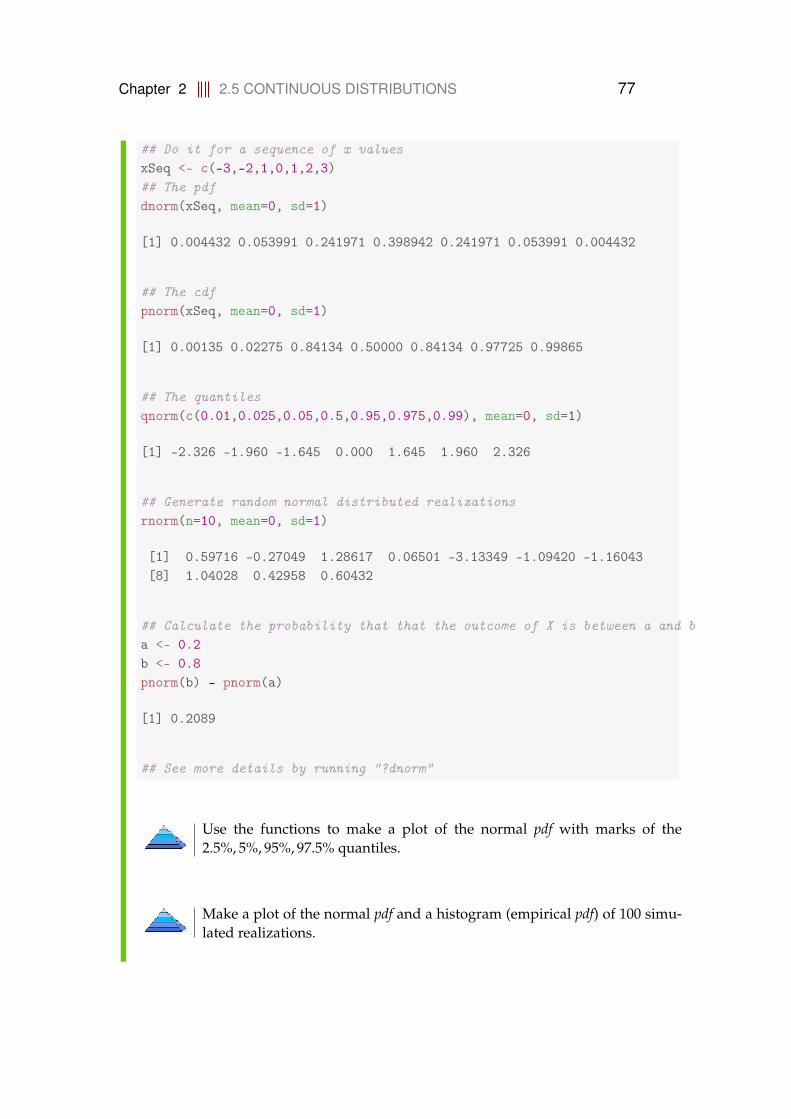
Chapter 2 2.5 CONTINUOUS DISTRIBUTIONS 77
## Do it for a sequence of x valuesxSeq <- c(-3,-2,1,0,1,2,3)## The pdfdnorm(xSeq, mean=0, sd=1)
[1] 0.004432 0.053991 0.241971 0.398942 0.241971 0.053991 0.004432
## The cdfpnorm(xSeq, mean=0, sd=1)
[1] 0.00135 0.02275 0.84134 0.50000 0.84134 0.97725 0.99865
## The quantilesqnorm(c(0.01,0.025,0.05,0.5,0.95,0.975,0.99), mean=0, sd=1)
[1] -2.326 -1.960 -1.645 0.000 1.645 1.960 2.326
## Generate random normal distributed realizationsrnorm(n=10, mean=0, sd=1)
[1] 0.59716 -0.27049 1.28617 0.06501 -3.13349 -1.09420 -1.16043[8] 1.04028 0.42958 0.60432
## Calculate the probability that that the outcome of X is between a and ba <- 0.2b <- 0.8pnorm(b) - pnorm(a)
[1] 0.2089
## See more details by running "?dnorm"
Use the functions to make a plot of the normal pdf with marks of the2.5%, 5%, 95%, 97.5% quantiles.
Make a plot of the normal pdf and a histogram (empirical pdf) of 100 simu-lated realizations.

Chapter 2 2.5 CONTINUOUS DISTRIBUTIONS 78
2.5.3 Log-Normal distribution
If a random variable is log-normal distributed then its logarithm is normallydistributed.
Definition 2.46 Log-Normal distribution
A log-normal distributed random variable
X ∼ LN(α, β2), (2-63)
where α is the mean and β2 is the variance of the normal distribution ob-tained when taking the natural logarithm to X.The log-normal pdf is
f (x) =1
x√
2πβe− (ln x−α)2
2β2 . (2-64)
Theorem 2.47 Mean and variance of log-normal distribution
Mean of the log-normal distribution
µ = eα+β2/2, (2-65)
and variance
σ2 = e2α+β2(eβ2 − 1). (2-66)
The log-normal distribution occurs in many fields, in particular: biology, fi-nance and many technical applications.
2.5.4 Exponential distribution
The usual application of the exponential distribution is for describing the length(usually time) between events which, when counted, follows a Poisson distri-bution, see Section 2.3.3. Hence the length between events which occur contin-
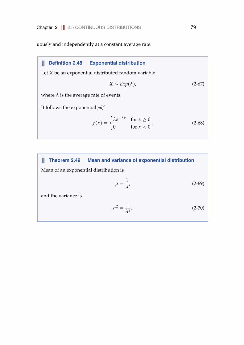
Chapter 2 2.5 CONTINUOUS DISTRIBUTIONS 79
uously and independently at a constant average rate.
Definition 2.48 Exponential distribution
Let X be an exponential distributed random variable
X ∼ Exp(λ), (2-67)
where λ is the average rate of events.
It follows the exponential pdf
f (x) =
{λe−λx for x ≥ 00 for x < 0
. (2-68)
Theorem 2.49 Mean and variance of exponential distribution
Mean of an exponential distribution is
µ =1λ
, (2-69)
and the variance is
σ2 =1
λ2 . (2-70)
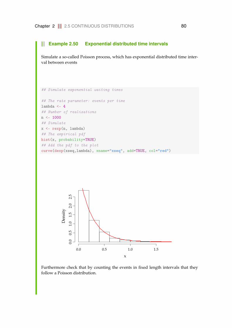
Chapter 2 2.5 CONTINUOUS DISTRIBUTIONS 80
Example 2.50 Exponential distributed time intervals
Simulate a so-called Poisson process, which has exponential distributed time inter-val between events
## Simulate exponential waiting times
## The rate parameter: events per timelambda <- 4## Number of realizationsn <- 1000## Simulatex <- rexp(n, lambda)## The empirical pdfhist(x, probability=TRUE)## Add the pdf to the plotcurve(dexp(xseq,lambda), xname="xseq", add=TRUE, col="red")
x
Den
sity
0.0 0.5 1.0 1.5
0.0
0.5
1.0
1.5
2.0
2.5
Furthermore check that by counting the events in fixed length intervals that theyfollow a Poisson distribution.

Chapter 2 2.5 CONTINUOUS DISTRIBUTIONS 81
## Check the relation to the Poisson distribution## by counting the events in each interval
## Sum up to get the running timexCum <- cumsum(x)## Use the hist function to count in intervals between the breaks,## here 0,1,2,...tmp <- hist(xCum, breaks=0:ceiling(max(xCum)))## Plot the discrete empirical pdfplot(table(tmp$counts)/length(tmp$counts))## Add the Poisson pdf to the plotlines(0:20, dpois(0:20,lambda), type="h", col="red")
0.00
0.10
0.20
0.30
x
Den
sity
0 1 2 3 4 5 6 7 8 9 10 11 12
Empirical pdfpdf
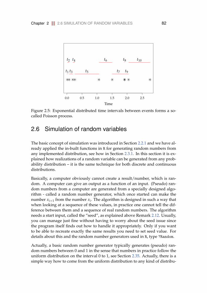
Chapter 2 2.6 SIMULATION OF RANDOM VARIABLES 82
0.0 0.5 1.0 1.5 2.0 2.5
Time
t1
t2
t3
t4
t5
t6
t7
t8
t9
t10
Figure 2.5: Exponential distributed time intervals between events forms a so-called Poisson process.
2.6 Simulation of random variables
The basic concept of simulation was introduced in Section 2.2.1 and we have al-ready applied the in-built functions in R for generating random numbers fromany implemented distribution, see how in Section 2.3.1. In this section it is ex-plained how realizations of a random variable can be generated from any prob-ability distribution – it is the same technique for both discrete and continuousdistributions.
Basically, a computer obviously cannot create a result/number, which is ran-dom. A computer can give an output as a function of an input. (Pseudo) ran-dom numbers from a computer are generated from a specially designed algo-rithm - called a random number generator, which once started can make thenumber xi+1 from the number xi. The algorithm is designed in such a way thatwhen looking at a sequence of these values, in practice one cannot tell the dif-ference between them and a sequence of real random numbers. The algorithmneeds a start input, called the “seed”, as explained above Remark 2.12. Usually,you can manage just fine without having to worry about the seed issue sincethe program itself finds out how to handle it appropriately. Only if you wantto be able to recreate exactly the same results you need to set seed value. Fordetails about this and the random number generators used in R, type ?Random.
Actually, a basic random number generator typically generates (pseudo) ran-dom numbers between 0 and 1 in the sense that numbers in practice follow theuniform distribution on the interval 0 to 1, see Section 2.35. Actually, there is asimple way how to come from the uniform distribution to any kind of distribu-

Chapter 2 2.6 SIMULATION OF RANDOM VARIABLES 83
tion:
Theorem 2.51
If U ∼ Uniform(0, 1) and F is a distribution function for any probabilitydistribution, then F−1(U) follow the distribution given by F
Recall, that the distribution function F in R is given by the p versions of thedistributions, while F−1 is given by the q versions.
Example 2.52 Random numbers in R
We can generate 100 normally distributed N(2, 32) numbers similarly the followingtwo ways:
## Generate 100 normal distributed valuesrnorm(100, mean=2, sd=3)## Similarly, generate 100 uniform distributed values from 0 to 1 and## put them through the inverse normal cdfqnorm(runif(100), mean=2, sd=3)
Example 2.53 Simulating the exponential distribution
Consider the exponential distribution with λ = 1/β = 1/2, that is, with densityfunction
f (x) = λe−λx,
for x > 0 and 0 otherwise. The distribution function is
F(x) =∫ x
0f (t)dt = 1− e−0.5x.
The inverse of this distribution function can be found by solving
u = 1− e−0.5x ⇔ x = −2 log(1− u).
So if random numbers U ∼ Uniform(0, 1) then −2 log(1−U) follows the exponen-tial distribution with λ = 1/2 (and β = 2). We confirm this in R here:
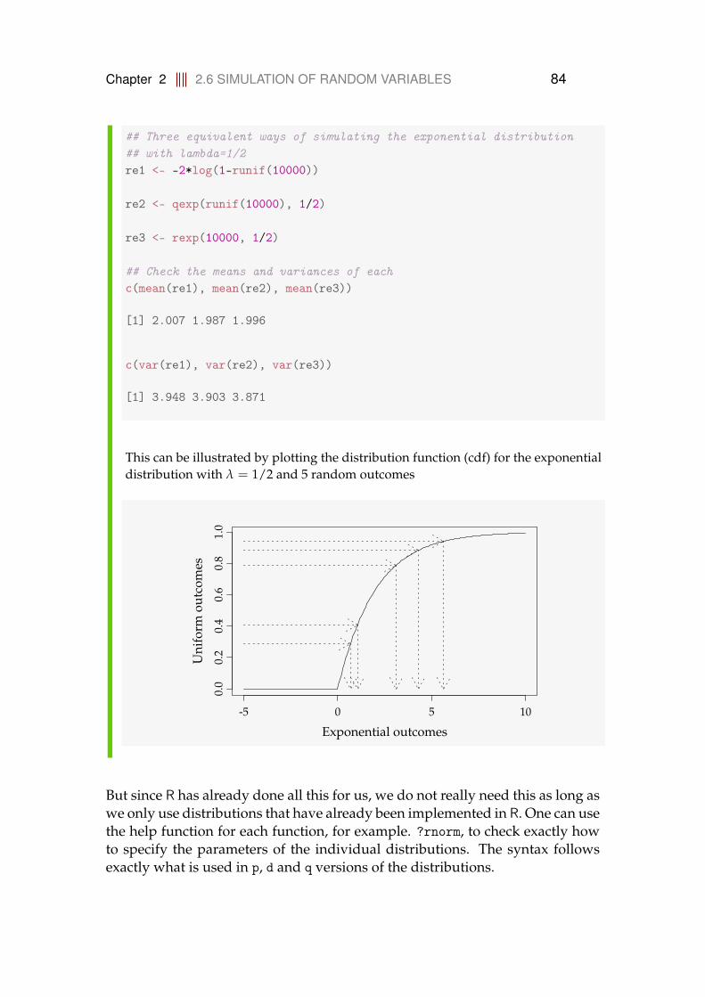
Chapter 2 2.6 SIMULATION OF RANDOM VARIABLES 84
## Three equivalent ways of simulating the exponential distribution## with lambda=1/2re1 <- -2*log(1-runif(10000))
re2 <- qexp(runif(10000), 1/2)
re3 <- rexp(10000, 1/2)
## Check the means and variances of eachc(mean(re1), mean(re2), mean(re3))
[1] 2.007 1.987 1.996
c(var(re1), var(re2), var(re3))
[1] 3.948 3.903 3.871
This can be illustrated by plotting the distribution function (cdf) for the exponentialdistribution with λ = 1/2 and 5 random outcomes
-5 0 5 10
0.0
0.2
0.4
0.6
0.8
1.0
Exponential outcomes
Uni
form
outc
omes
But since R has already done all this for us, we do not really need this as long aswe only use distributions that have already been implemented in R. One can usethe help function for each function, for example. ?rnorm, to check exactly howto specify the parameters of the individual distributions. The syntax followsexactly what is used in p, d and q versions of the distributions.
Chapter 2 2.7 IDENTITIES FOR THE MEAN AND VARIANCE 85
2.7 Identities for the mean and variance
Rules for calculation of the mean and variance of linear combinations of in-dependent random variables are introduced here. They are valid for both thediscrete and continuous case.
Theorem 2.54 Mean and variance of linear functions
Let Y = aX + b then
E(Y) = E(aX + b) = a E(X) + b, (2-71)
and
V(Y) = V(aX + b) = a2 V(X). (2-72)
Random variables are often scaled (i.e. aX) for example when shifting units:
Example 2.55
The mean of a bike shops sale is 100 bikes per month and varies with a standarddeviation of 15. They earn 200 Euros per bike. What is the mean and standarddeviation of their earnings per month?
Let X be the number of bikes sold per month. On average they sell µX = 100 bikesper month and it varies with a variance of σ2
X = 225. The shops monthly earnings
Y = 200X,
has then a mean and standard deviation of
µY = E(Y) = E(200X) = 200 E(X) = 200 · 100 = 20000 Euro/month,
σY =√
V(Y) =√
V(200X) =√
2002 V(X) =√
40000 · 225 = 3000 Euro/month.
Chapter 2 2.7 IDENTITIES FOR THE MEAN AND VARIANCE 86
Theorem 2.56 Mean and variance of linear combinations
The mean of a linear combination of independent random variables is
E(a1X1 + a2X2 + · · ·+ anXn) = a1 E(X1) + a2 E(X2) + · · ·+ an E(Xn),(2-73)
and the variance
V(a1X1 + a2X2 + · · ·+ anXn) = a21 V(X1) + a2
2 V(X2) + · · ·+ a2n V(Xn).
(2-74)
Example 2.57
Lets take a dice example to emphasize an important point. Let Xi represent theoutcome of a roll with a dice with mean µX and standard deviation σX.
Now, consider a scaling of a single roll with a dice, say five times
Yscale = 5X1,
then the mean will scale linearly
E(Yscale) = E(5X1) = 5 E(X1) = 5 µX,
and the standard deviation also scales linearly
σ2Yscale = V(5X1) = 52 V(X1) = 52 σ2
X ⇔ σYscale = 5 σX.
Whereas for a sum of five rolls
Ysum = X1 + X2 + X3 + X4 + X5,
the mean will similarly scale linearly
E(Ysum) = E(X1 + X2 + X3 + X4 + X5)
= E(X1) + E(X2) + E(X3) + E(X4) + E(X5)
= 5 µX,
however the standard deviation will increase only with the square root
σ2Ysum = V(X1 + X2 + X3 + X4 + X5)
= V(X1) + V(X2) + V(X3) + V(X4) + V(X5)
= 5 σ2X ⇔
σYsum =√
5 σX.

Chapter 2 2.7 IDENTITIES FOR THE MEAN AND VARIANCE 87
This is simply because when applying the sum to many random outcomes, thenthe high and low outcomes will even out each other, such that the variance will besmaller for a sum than for a scaling.
Chapter 2 2.8 COVARIANCE AND CORRELATION 88
2.8 Covariance and correlation
In this chapter we have discussed mean and variance (or standard deviation),and the relation to the sample mean and sample variance, see Section 2.2.2. InChapter 1 Section 1.4.3 we discussed the sample covariance and sample correla-tion, these two measures also have theoretical justification, namely covarianceand correlation, which we will discuss in this section. We start by the definitionof covariance.
Definition 2.58 Covariance
Let X and Y be two random variables, then the covariance between X andY, is
Cov(X, Y) = E[(X− E[X])(Y− E[Y])] . (2-75)
Remark 2.59
It follows immediately from the definition that Cov(X, X) = V(X) andCov(X, Y) = Cov(Y, X).
An important concept in statistics is independence (see Section 2.9 for a formaldefinition). We often assume that realizations (random variables) are indepen-dent. If two random variables are independent then their covariance will bezero, the reverse is however not necessarily true (see also the discussion onsample correlation in Section 1.4.3).
The following calculation rule apply to covariance between two random vari-ables X and Y:
Theorem 2.60 Covariance between linear combinations
Let X and Y be two random variables, then
Cov(a0 + a1X + a2Y, b0 + b1X + b2Y) = a1b1 V(X) + a2b2 V(Y) + (a1b2 + a2b1)Cov(X, Y).(2-76)
Chapter 2 2.8 COVARIANCE AND CORRELATION 89
Proof
Let Z1 = a0 + a1X + a2Y and Z2 = b0 + b1X + b2Y then
Cov(Z1, Z2) = E[(a1(X− E[X]) + a2(Y− E[Y]))(b1(X− E[X]) + b2(Y− E[Y]))]
= E[a1(X− E[X])b1(X− E[X])] + E[a1(X− E[X])b2(Y− E[Y])]+
E[a2(Y− E[Y])b1(X− E[X])] + E[a2(Y− E[Y])b2(Y− E[Y])]
= a1b1 V(X) + a2b2 V(Y) + (a1b2 + a2b2)Cov(X, Y). (2-77)
�
Example 2.61
Let X ∼ N(3, 22) and Y ∼ N(2, 1) and the covariance between X and Y given byCov(X, Y) = 1. What is the variance of the random variable Z = 2X−Y?
V(Z) = Cov[2X−Y, 2X−Y] = 22 V(X) + V(Y)− 4 Cov(X, Y)
= 2222 + 1− 4 = 13.
We have already seen in Section 1.4.3 that the sample correlation measures theobserved degree of linear dependence between two random variables – calcu-lated from samples observed on the same observational unit e.g. height andweight of persons. The theoretical counterpart is the correlation between tworandom variables – the true linear dependence between the two variables:
Definition 2.62 Correlation
Let X and Y be two random variables with V(X) = σ2x , V(Y) = σ2
y , andCov(X, Y) = σxy, then the correlation between X and Y is
ρxy =σxy
σxσy. (2-78)
Remark 2.63
The correlation is a number between -1 and 1.
Chapter 2 2.8 COVARIANCE AND CORRELATION 90
Example 2.64
Let X ∼ N(1, 22) and ε ∼ N(0, 0.52) be independent random variables, find thecorrelation between X and Z = X + ε.
The variance of Z is
V(Z) = V(X + ε) = V(X) + V(ε) = 4 + 0.25 = 4.25.
The covariance between X and Z is
Cov(X, Z) = Cov(X, X + ε) = V(X) = 4,
and hence
ρxz =4√
4.25 · 4= 0.97.
Chapter 2 2.9 INDEPENDENCE OF RANDOM VARIABLES 91
2.9 Independence of random variables
In statistics the concept of independence is very important, and in order togive a formal definition of independence we will need the definition of two-dimensional random variables. The probability density function of a two-dimensionaldiscrete random variable, called the joint probability density function, is,
Definition 2.65 Joint pdf of two-dimensional discrete random vari-ables
The pdf of a two-dimensional discrete random variable [X, Y] is
f (x, y) = P(X = x, Y = y), (2-79)
with the properties
f (x, y) ≥ 0 for all (x, y), (2-80)
∑all x
∑all y
f (x, y) = 1. (2-81)
Remark 2.66
P(X = x, Y = y) should be read: the probability of X = x and Y = y.
Example 2.67
Imagine two throws with an fair coin: the possible outcome of each throw is eitherhead or tail, which will be given the values 0 and 1 respectively. The complete set ofoutcomes is (0,0), (0,1), (1,0), and (1,1) each with probability 1/4. And hence the pdfis
f (x, y) =14
; x = {0, 1}, y = {0, 1},
further we see that1
∑x=0
1
∑y=0
f (x, y) =1
∑x=0
( f (x, 0) + f (x, 1)) = f (0, 0) + f (0, 1) + f (1, 0) + f (1, 1)
= 1.

Chapter 2 2.9 INDEPENDENCE OF RANDOM VARIABLES 92
The formal definition of independence for a two dimensional discrete randomvariable is:
Definition 2.68 Independence of discrete random variables
Two discrete random variables X and Y are said to be independent if andonly if
P(X = x, Y = y) = P(X = x)P(Y = y). (2-82)
Example 2.69
Example 2.67 is an example of two independent random variables, to see this writethe probabilities
P(X = 0) =1
∑y=0
f (0, y) =12
,
P(X = 1) =1
∑y=0
f (1, y) =12
.
similarly P(Y = 0) = 12 and P(Y = 1) = 1
2 , now we see that P(X = x)P(Y = y) = 14
for all possible x and y, and hence
P(X = x)P(Y = y) = P(X = x, Y = y) =14
.
Example 2.70
Now imagine that for the second throw we don’t see the outcome of Y, but onlyobserve the sum of X and Y, denote it by
Z = X + Y.
Lets find out if X and Z are independent. In this case the for all outcomes (0, 0),(0, 1), (1, 1), (1, 2) the joint pdf is
P(X = 0, Z = 0) = P(X = 0, Z = 1) = P(X = 1, Z = 1) = P(X = 1, Z = 2) =14
.
The pdf for each variable is: for X
P(X = 0) = P(X = 1) =12
,

Chapter 2 2.9 INDEPENDENCE OF RANDOM VARIABLES 93
and for Z
P(Z = 0) = P(Z = 2) =14
and P(Z = 1) =12
,
thus for example for the particular outcome (0, 0)
P(X = 0)P(Z = 0) =12· 1
4=
186= 1
4= P(X = 0, Z = 0),
the pdf s are not equal and hence we see that X and Z are not independent.
Remark 2.71
In the example above it is quite clear that X and Z cannot be independent.In real applications we do not know exactly how the outcomes are realizedand therefore we will need to assume independence (or test it).
To be able to define independence of continuous random variables, we will needthe pdf of a two-dimensional random variable:
Definition 2.72 Pdf of two dimensional continous random vari-ables
The pdf of a two-dimensional continous random variable [X, Y] is a functionf (x, y) from R2 into R+ with the properties
f (x, y) ≥ 0 for all (x, y), (2-83)∫ ∫
f (x, y)dxdy = 1. (2-84)
Just as for one-dimensional random variables the probability interpretation isin form of integrals
P((X, Y) ∈ A
)=∫
Af (x, y)dxdy, (2-85)
where A is an area.
Chapter 2 2.9 INDEPENDENCE OF RANDOM VARIABLES 94
Example 2.73 Bivariate normal distribution
The most important two-dimensional distribution is the bivariate normal distribu-tion
f (x1, x2) =1
2π√|Σ|
e−12 (x−µ)TΣ−1(x−µ)
=1
2π√
σ11σ22 − σ212
e− σ2
22(x1−µ1)2+σ22(x2−µ2)
2−2σ12(x1−µ1)(x2−µ2)
2(σ11σ22−σ212) ,
where x = (x1, x2), and µ = [E(X1), E(X2)], and Σ is the so-called variance-covariance matrix with elements (Σ)ij = σij = Cov(Xi, Xj), note that σ12 = σ21,| · | is the determinant, and Σ−1 is the inverse of Σ.
Definition 2.74 Independence of continous random variables
Two continous random variables X and Y are said to be independent if
f (x, y) = f (x) f (y). (2-86)
We list here some properties of independent random variables.
Theorem 2.75 Properties of independent random variables
If X and Y are independent then
E(XY) = E(X)E(Y), (2-87)
and
Cov(X, Y) = 0. (2-88)
Let X1, . . . , Xn be independent and identically distributed random variablesthen
Cov(X, Xi − X) = 0. (2-89)
Chapter 2 2.9 INDEPENDENCE OF RANDOM VARIABLES 95
Proof
E(XY) =∫ ∫
xy f (x, y)dxdy =∫ ∫
xy f (x) f (y)dxdy
=∫
x f (x)dx∫
y f (y)dy = E(X)E(Y)(2-90)
Cov(X, Y) = E[(X− E(X))(Y− E(Y))]
= E[XY]− E[E(X)Y]− E[X E(Y)] + E(X)E(Y)
= 0.
(2-91)
Cov(X, Xi − X) = Cov(X, Xi)−Cov(X, X)
=1n
σ2 − 1n2 Cov
(∑ Xi, ∑ Xi
)
=1n
σ2 − 1n2 nσ2 = 0.
(2-92)
�
Remark 2.76
Note that Cov(X, Y) = 0 does not imply that X and Y are independent.However, if X and Y follow a bivariate normal distribution, then if X and Yare uncorrelated then they are also independent.

Chapter 2 2.10 FUNCTIONS OF NORMAL RANDOM VARIABLES 96
2.10 Functions of normal random variables
This section will cover some important functions of a normal random variable.In general the question of how an arbitrary function of a random variable is dis-tributed cannot be answered on closed form (ı.e. directly and exactly calculated)– for answering such questions we must use simulation as a tool, as covered de-tails in Chapter 4. We have already discussed simulation as a learning tool,which will also be used in this section.
The simplest function we can think of is a linear combination of normal randomvariables, which we from Theorem 2.40 know will follow a normal distribution.The mean and variance of this normal distribution can be calculated using theidentities given in Theorem 2.56.
Remark 2.77
Note that combining Theorems 2.40 and 2.75, and Remark 2.76 imply that Xand Xi − X are independent.
In addition to the result given above we will cover three additional distribu-tions: χ2-distribution, t-distribution and the F-distribution, which are all veryimportant for the statistical inference covered in the following chapters.

Chapter 2 2.10 FUNCTIONS OF NORMAL RANDOM VARIABLES 97
2.10.1 The χ2-distribution
The χ2-distribution (chi-square) is defined by:
Definition 2.78
Let X be χ2 distributed, then its pdf is
f (x) =1
2ν2 Γ(
ν2
) xν2−1e−
x2 ; x ≥ 0, (2-93)
where Γ(
ν2
)is the Γ-function and ν is the degrees of freedom.
An alternative definition (here formulated as a theorem) of the χ2-distributionis:
Theorem 2.79
Let Z1, . . . , Zνbe independent random variables following the standard nor-mal distribution, then
ν
∑i=1
Z2i ∼ χ2(ν). (2-94)
We will omit the proof of the theorem as it requires more probabilty calculusthan covered here. Rather a small example that illustrates how the theorem canbe checked by simulation:

Chapter 2 2.10 FUNCTIONS OF NORMAL RANDOM VARIABLES 98
Example 2.80 simulation of χ2-distribution
## Simulate 10 realizations from a standard normal distributed variablen <- 10rnorm(n)## Now repeat this 200 times and calculate the sum of squares each time## Note: the use of the function replicate: it repeats the## expression in the 2nd argument k times, see ?replicatek <- 200x <- replicate(k, sum(rnorm(n)^2))## Plot the epdf of the sums and compare with the theoretical chisquare pdfpar(mfrow=c(1,2))hist(x, freq=FALSE)curve(dchisq(xseq,df=n), xname="xseq", add=TRUE, col="red")## and the ecdf compared to the cdfplot(ecdf(x))curve(pchisq(xseq,df=n), xname="xseq", add=TRUE, col="red")
x
Den
sity
5 10 15 20 25 30
0.00
0.02
0.04
0.06
0.08
0.10
epdfpdf
5 10 15 20 25 30
0.0
0.2
0.4
0.6
0.8
1.0
ecdf(x)
x
Cum
ulat
edde
nsit
y
ecdfcdf
In the left plot the empirical pdf is compared to the theoretical pdf and in the rightplot the empirical cdf is compared to the theoretical cdf.
Chapter 2 2.10 FUNCTIONS OF NORMAL RANDOM VARIABLES 99
Theorem 2.81
Given a sample of size n from the normal distributed random variables Xiwith variance σ2, then the sample variance S2 (viewed as random variable)can be transformed into
χ2 =(n− 1)S2
σ2 , (2-95)
which follows the χ2-distribution with degrees of freedom ν = n− 1.
Proof
Start by rewriting the expression
(n− 1)S2
σ2 =n
∑i=1
(Xi − X
σ
)2
=n
∑i=1
(Xi − µ + µ− X
σ
)2
=n
∑i=1
(Xi − µ
σ
)2
+n
∑i=1
(X− µ
σ
)2
− 2n
∑i=1
(X− µ)(Xi − µ)
σ2
=n
∑i=1
(Xi − µ
σ
)2
+ n(
X− µ
σ
)2
− 2n(
X− µ
σ
)2
=n
∑i=1
(Xi − µ
σ
)2
−(
X− µ
σ/√
n
)2
,
(2-96)
we know that Xi−µσ ∼ N(0, 1) and X−µ
σ/√
n ∼ N(0, 1), and hence the left hand side is a
χ2(n) distributed random variable minus a χ2(1) distributed random variable (alsoX and S2 are independent, see Theorems 2.75, and 2.40, and Remark 2.76). Hencethe left hand side must be χ2(n− 1).
�
If someone claims that a sample comes from a specific normal distribution (i.e.Xi ∼ N(µ, σ2), then we can examine probabilities of specific outcomes of thesample variance. Such calculation will be termed hypethesis test in later chap-ters.
Chapter 2 2.10 FUNCTIONS OF NORMAL RANDOM VARIABLES 100
Example 2.82 Milk dose machines
A manufacture of machines for dosing milk claims that their machines can dose witha precision defined by the normal distribution with a standard deviation less than2% of the dose volume in the operation range. A sample of n = 20 observations wastaken to check if the precision was as claimed. The sample standard deviation wascalculated to s = 0.03.
Hence the claim is that σ ≤ 0.02, thus we want to answer the question: if σ = 0.02(i.e. the upper limit of the claim), what is then the probability of getting the samplingdeviation s ≥ 0.03?
## Chi-square milk dosing precision
## The sample sizen <- 20## The claimed deviationsigma <- 0.02## The observed sample standard deviations <- 0.03## Calculate the chi-square statisticchiSq <- (n-1)*s^2 / sigma^2## Use the cdf to calculate the probability of getting the observed## sample standard deviation or higher1 - pchisq(chiSq, df=n-1)
[1] 0.001402
It seems very unlikely that the standard deviation is below 0.02 since the probabilityof obtaining the observed sample standard deviation under this condition is verysmall. The probability we just found will be termed a p-value in later chapters - thep-value a very fundamental in testing of hypothesis.
The probability calculated in the above example will be called the p-value inlater chapters and it is a very fundamental concept in statistics.
Theorem 2.83 Mean and variance
Let X ∼ χ2(ν) then the mean and variance of X is
E(X) = ν; V(X) = 2ν. (2-97)
Chapter 2 2.10 FUNCTIONS OF NORMAL RANDOM VARIABLES 101
We will omit the proof of this theorem, but it is easily checked by a symboliccalculation software (like e.g. Maple).
Example 2.84
We want to calculate the expected value of the sample variance (S2) based on nobservations with Xi ∼ N(µ, σ2). We have already seen that n−1
σ2 S2 ∼ χ2(n− 1) andwe can therefore write
E(S2) =σ2
n− 1n− 1
σ2 E(S2)
=σ2
n− 1E(
n− 1σ2 S2
)
=σ2
n− 1(n− 1) = σ2,
and we say that S2 is a central estimator for σ2 (the term estimator is introduced inSection 3.1.3). We can also find the variance of the estimator
V(S2) =
(σ2
n− 1
)2
V(
n− 1σ2 S2
)
=σ4
(n− 1)2 2(n− 1) = 2σ4
n− 1.
Example 2.85 Pooled variance
Suppose now that we have two different samples (not yet realized) X1, . . . , Xn1 andY1, . . . , Yn2 with Xi ∼ N(µ1, σ2) and Yi ∼ N(µ2, σ2) (both i.i.d.). Let S2
1 be the samplevariance based on the X’s and S2
2 be the sample variance based on the Y’s. Now bothS2
1 and S22 will be central estimators for σ2, and so will any weighted average of the
type
S2 = aS21 + (1− a)S2
2; a ∈ [0, 1].
Now we would like to choose a such that the variance of S2 is as small as possible,and hence we calculate the variance of S2
V(S2) = a22σ4
n1 − 1+ (1− a)22
σ4
n2 − 1
= 2σ4(
a2 1n1 − 1
+ (1− a)2 1n2 − 1
).
Chapter 2 2.10 FUNCTIONS OF NORMAL RANDOM VARIABLES 102
In order to find the minimum we differentiate with respect to a
∂ V(S2)
∂a= 2σ4
(2a
1n1 − 1
− 2(1− a)1
n2 − 1
)
= 4σ4(
a(
1n1 − 1
+1
n2 − 1
)− 1
n2 − 1
)
= 4σ4(
an1 + n2 − 2
(n1 − 1)(n2 − 1)− 1
n2 − 1
),
which is zero for
a =n1 − 1
n1 + n2 − 2.
In later chapters we will refer to this choice of a as the pooled variance (S2p), inserting
in (2-98) gives
S2p =
(n1 − 1)S21 + (n2 − 1)S2
2n1 + n2 − 2
.
Note that S2p is a weighted (proportional to the number of observations) average
of the sample variances. It can also be shown (you are invited to do this) thatn1+n2−2
σ2 S2p ∼ χ2(n1 + n2 − 2). Further, note that the assumption of equal variance in
the two samples is crucial in the calculations above.
2.10.2 The t-distribution
The t-distribution is the sampling distribution of the sample mean standardizedwith the sample variation. It is valid for all sample sizes, however for largersample sizes (n > 30) the difference between the t-distribution and the normaldistribution is very small. Hence for larger sample sizes the normal distributionis often applied.
Definition 2.86
The t-distribution pdf is
fT(t) =Γ( ν+1
2 )√νπ Γ( ν
2)
(1 + t2
ν
)− ν+12 , (2-98)
where ν is the degrees of freedom and Γ() is the Gamma function.

Chapter 2 2.10 FUNCTIONS OF NORMAL RANDOM VARIABLES 103
The relation between normal random variables and χ2-distributed random vari-ables are given in the following theo:rem
Theorem 2.87
Let Z ∼ N(0, 1) and Y ∼ χ2(ν), then
X =Z√Y/ν
∼ t(ν). (2-99)
We will not prove this theorem, but show by an example how this can be illus-trated by simulation:
Example 2.88 Relation between normal and χ2
## Set simulate parametersnu <- 8; k <- 200## Generate the simulated realizationsz <- rnorm(k)y <- rchisq(k, df=nu)x <- z/sqrt(y/nu)## Plotpar(mfrow=c(1,2))hist(x, freq = FALSE)curve(dt(xseq, df = nu), xname="xseq", add=TRUE, col="red")plot(ecdf(x))curve(pt(xseq, df = nu), xname="xseq", add=TRUE, col="red")
x
Den
sity
-4 -2 0 2 4
0.0
0.1
0.2
0.3
0.4
epdfpdf
-4 -2 0 2 4
0.0
0.2
0.4
0.6
0.8
1.0
ecdf(x)
x
Cum
ulat
edde
nsit
y
ecdfcdf
Chapter 2 2.10 FUNCTIONS OF NORMAL RANDOM VARIABLES 104
In the left plot the empirical pdf is compared to the theoretical pdf and in the rightplot the empirical cdf is compared to the theoretical cdf.
The t-distribution arises when a sample is taken of a normal distributed randomvariable, then the sample mean standardized with the sample variance followsthe t-distribution.
Theorem 2.89
Given a sample of normal distributed random variables X1, . . . , Xn, then therandom variable
T =X− µ
S/√
n∼ t(n− 1), (2-100)
follows the t-distribution, where X is the sample mean, µ is the mean of X,n is the sample size and S is the sample standard deviation.
Proof
Note that X−µ
σ/√
n ∼ N(0, 1) and (n−1)S2
σ2 ∼ χ2(n− 1) which inserted in Equation (2.87)gives
T =
X−µ
σ/√
n√(n−1)S2
σ2(n−1)
=
X−µ
1/√
n√S2
=X− µ
S/√
n∼ t(n− 1).
(2-101)
�
We could also verify this by simulation:

Chapter 2 2.10 FUNCTIONS OF NORMAL RANDOM VARIABLES 105
Example 2.90 Simulation of t-distribution
## Simulaten <- 8; k <- 200; mu <- 1; sigma <- 2## Repeat k times the simulation of a normal dist. sample:## return the values in a (n x k) matrixx <- replicate(k, rnorm(n, mean=mu, sd=sigma))xbar <- apply(x, 2, mean)s <- apply(x, 2, sd)tobs <- (xbar - mu)/(s/sqrt(n))## Plotpar(mfrow=c(1,2))hist(tobs, freq = FALSE)curve(dt(xseq, df=n-1), xname="xseq", add=TRUE, col="red")plot(ecdf(tobs))curve(pt(xseq, df=n-1), xname="xseq", add=TRUE, col="red")
tobs
Den
sity
-4 -2 0 2 4
0.0
0.1
0.2
0.3
0.4
epdfpdf
-4 -2 0 2 4
0.0
0.2
0.4
0.6
0.8
1.0
tobs
Cum
ulat
edde
nsit
y
ecdfcdf
In the left plot the empirical pdf is compared to the theoretical pdf and in the rightplot the empirical cdf is compared to the theoretical cdf.
Note that X and S are random variables, since they are the sample mean andstandard deviation of a sample consisting of realizations of X, but the sample isnot taken yet.
Very often samples with only few observations are available. In this case byassuming normality of the population (i.e. the Xi’s are normal distributed) andfor a some mean µ, the t-distribution can be used to calculate the probability ofobtaining the sample mean in a given range.

Chapter 2 2.10 FUNCTIONS OF NORMAL RANDOM VARIABLES 106
Example 2.91 Electric car driving distance
An electric car manufacture claims that their cars can drive on average 400 km ona full charge at a specified speed. From experience it is known that this full chargedistance, denote it by X, is normal distributed. A test of n = 10 cars was carried out,which resulted in a sample mean of x = 382 km and a sample deviation of s = 14.
Now we can use the t-distribution to calculate the probability of obtaining this valueof the sample mean or lower, if their claim about the mean is actually true:
## Calculate the probability of getting the sample mean under the## conditions that the claim is actually the real mean
## A test of 10 cars was carried outn <- 10## The claim is that the real mean is 400 kmmuX <- 400## From the sample the sample mean was calculated toxMean <- 393## And the sample deviation wasxSD <- 14## Use the cdf to calculate the probability of obtaining this## sample mean or a lower valuept( (xMean-muX) / (xSD/sqrt(n)), df=n-1)
[1] 0.07415
If we had the same sample mean and sample deviation, how do you thinkchanging the number of observations will affect the calculated probability?Try it out.
The t-distribution converges to the normal distribution as the simple size in-creases. For small sample sizes it has a higher spread than the normal distribu-tion. For larger sample sizes with n > 30 observations the difference betweenthe normal and the t-distribution is very small.
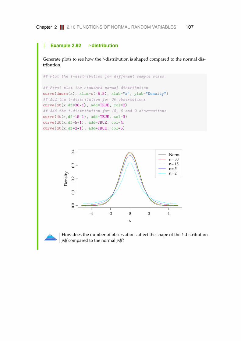
Chapter 2 2.10 FUNCTIONS OF NORMAL RANDOM VARIABLES 107
Example 2.92 t-distribution
Generate plots to see how the t-distribution is shaped compared to the normal dis-tribution.
## Plot the t-distribution for different sample sizes
## First plot the standard normal distributioncurve(dnorm(x), xlim=c(-5,5), xlab="x", ylab="Density")## Add the t-distribution for 30 observationscurve(dt(x,df=30-1), add=TRUE, col=2)## Add the t-distribution for 15, 5 and 2 observationscurve(dt(x,df=15-1), add=TRUE, col=3)curve(dt(x,df=5-1), add=TRUE, col=4)curve(dt(x,df=2-1), add=TRUE, col=5)
-4 -2 0 2 4
0.0
0.1
0.2
0.3
0.4
x
Den
sity
Norm.n= 30n= 15n= 5n= 2
How does the number of observations affect the shape of the t-distributionpdf compared to the normal pdf?
Chapter 2 2.10 FUNCTIONS OF NORMAL RANDOM VARIABLES 108
Theorem 2.93 Mean and variance
Let X ∼ t(ν) then the mean and variance of X is
E(X) = 0; ν > 1, (2-102)
V(X) =ν
ν− 2; ν > 2. (2-103)
We will omit the proof of this theorem, but it is easily checked with a symboliccalculation software (like e.g. Maple).
Remark 2.94
For ν ≤ 1 the expectation (and hence the variance) is not defined (the inte-gral is not absolutely convergent), and for ν ∈ (1, 2] (1 < ν ≤ 2) the varianceis equal ∞. Note that this does not violate the general definition of probabil-ity density functions.
2.10.3 The F-distribution
The F-distribution is defined by:
Definition 2.95
The F-distribution pdf is
fF(x) =1
B( ν1
2 , ν22
)(
ν1
ν2
) ν12
xν12 −1
(1 +
ν1
ν2x)− ν1+ν2
2
, (2-104)
where ν1 an ν2 are the degrees of freedom and B(·, ·) is the Beta function.
The F-distribution appears as the ratio between two independent χ2-distributedrandom variables:
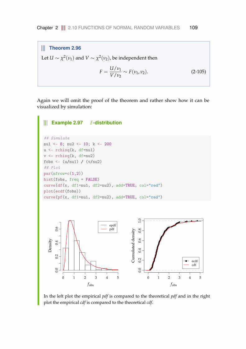
Chapter 2 2.10 FUNCTIONS OF NORMAL RANDOM VARIABLES 109
Theorem 2.96
Let U ∼ χ2(ν1) and V ∼ χ2(ν2), be independent then
F =U/ν1
V/ν2∼ F(ν1, ν2). (2-105)
Again we will omit the proof of the theorem and rather show how it can bevisualized by simulation:
Example 2.97 F-distribution
## Simulatenu1 <- 8; nu2 <- 10; k <- 200u <- rchisq(k, df=nu1)v <- rchisq(k, df=nu2)fobs <- (u/nu1) / (v/nu2)## Plotpar(mfrow=c(1,2))hist(fobs, freq = FALSE)curve(df(x, df1=nu1, df2=nu2), add=TRUE, col="red")plot(ecdf(fobs))curve(pf(x, df1=nu1, df2=nu2), add=TRUE, col="red")
fobs
Den
sity
0 1 2 3 4 5
0.0
0.2
0.4
0.6
epdfpdf
0 1 2 3 4 5
0.0
0.2
0.4
0.6
0.8
1.0
fobs
Cum
ulat
edde
nsit
y
ecdfcdf
In the left plot the empirical pdf is compared to the theoretical pdf and in the rightplot the empirical cdf is compared to the theoretical cdf.
Chapter 2 2.10 FUNCTIONS OF NORMAL RANDOM VARIABLES 110
Theorem 2.98
Let X1, . . . , Xn1 be independent and sampled from a normal distributionwith mean µ1 and variance σ2
1 , further let Y1, . . . , Yn2 be independent andsampled from a normal distribution with mean µ2 and variance σ2
2 . Thenthe statistic
F =S2
1/σ21
S22/σ2
2∼ F(n1 − 1, n2 − 1), (2-106)
follows an F-distribution.
Proof
Note that (n1−1)S21
σ21∼ χ2(n1 − 1) and (n2−1)S2
2σ2
2∼ χ2(n2 − 1) and hence
(n1−1)S21
σ21 (n1−1)
(n2−1)S22
σ22 (n2−1)
=
S21
σ21
S22
σ22
∼ F(n1 − 1, n2 − 1). (2-107)
�
We can also illustrate this sample version by simulation:
Example 2.99 Relation between normal and F-distribution
## Simulaten1 <- 8; n2 <- 10; k <- 200mu1 <- 2; mu2 <- -1sigma1 <- 2; sigma2 <- 4s1 <- replicate(k, sd(rnorm(n1, mean=mu1, sd=sigma1)))s2 <- replicate(k, sd(rnorm(n2, mean=mu2, sd=sigma2)))fobs <- (s1^2 / sigma1^2) / (s2^2 / sigma2^2)## Plotpar(mfrow=c(1,2))hist(fobs, freq=FALSE)curve(df(xseq, df1=n1-1, df2=n2-1), xname="xseq", add=TRUE, col="red")plot(ecdf(fobs))curve(pf(xseq, df1=n1-1, df2=n2-1), xname="xseq", add=TRUE, col="red")

Chapter 2 2.10 FUNCTIONS OF NORMAL RANDOM VARIABLES 111
fobs
Den
sity
0 1 2 3 4 5 6
0.0
0.2
0.4
0.6 epdf
0 2 4 6
0.0
0.2
0.4
0.6
0.8
1.0
fobs
Cum
ulat
edde
nsit
y
ecdfcdf
In the left plot the empirical pdf is compared to the theoretical pdf and in the rightplot the empirical cdf is compared to the theoretical cdf.
Remark 2.100
Of particular importance in statistics is the case when σ1 = σ2, in this case
F =S2
1S2
2∼ F(n1 − 1, n2 − 1). (2-108)
Theorem 2.101 Mean and variance
Let F ∼ F(ν1, ν2) then the mean and variance of F is
E(F) =ν2
ν2 − 2; ν2 > 2, (2-109)
V(F) =2ν2
2(ν1 + ν2 − 2)ν1(ν2 − 2)2(ν2 − 4)
; ν2 > 4. (2-110)
Chapter 2 2.11 EXERCISES 112
2.11 Exercises
Exercise 2.1 Discrete random variable
a) Let X be a stochastic variable. When running the R-command dbinom(4,10,0.6)R returns 0.1115, written as:
dbinom(4,10,0.6)
[1] 0.1115
What distribution is applied and what does 0.1115 represent?
b) Let X be the same stochastic variable as above. The following are resultsfrom R:
pbinom(4,10,0.6)
[1] 0.1662
pbinom(5,10,0.6)
[1] 0.3669
Calculate the following probabilities: P(X ≤ 5), P(X < 5), P(X > 4) andP(X = 5).
c) Let X be a stochastic variable. From R we get:
dpois(4,3)
[1] 0.168
What distribution is applied and what does 0.168 represent?
d) Let X be the same stochastic variable as above. The following are resultsfrom R:

Chapter 2 2.11 EXERCISES 113
ppois(4,3)
[1] 0.8153
ppois(5,3)
[1] 0.9161
Calculate the following probabilities: P(X ≤ 5), P(X < 5), P(X > 4) andP(X = 5).
Exercise 2.2 Course passing proportions
a) If a passing proportion for a course given repeatedly is assumed to be 0.80on average, and there are 250 students who are taking the exam each time,what is the expected value, µ and standard deviation, σ, for the numberof students who do not pass the exam for a randomly selected course?
Exercise 2.3 Notes in a box
A box contains 6 notes:
On 1 of the notes there is the number 1On 2 of the notes there is the number 2On 2 of the notes there is the number 3On 1 of the notes there is the number 4
Two notes are drawn at random from the box, and the following random vari-able is introduced: X, which describes the number of notes with the number 4among the 2 drawn. The two notes are drawn without replacement.
a) The mean and variance for X, and P(X = 0) are?
b) The 2 notes are now drawn with replacement. What is the probability thatnone of the 2 notes has the number 1 on it?
Chapter 2 2.11 EXERCISES 114
Exercise 2.4 Consumer survey
In a consumer survey performed by a newspaper, 20 different groceries (prod-ucts) were purchased in a grocery store. Discrepancies between the price ap-pearing on the sales slip and the shelf price were found in 6 of these purchasedproducts.
a) At the same time a customer buys 3 random (different) products withinthe group consisting of the 20 goods in the store. The probability that nodiscrepancies occurs for this customer is?
Exercise 2.5 Hay delivery quality
A horse owner receives 20 bales of hay in a sealed plastic packaging. To con-trol the hay, 3 bales of hay are randomly selected, and each checked whether itcontains harmful fungal spores.
It is believed that among the 20 bales of hay 2 bales are infected with fungalspores. A random variable X describes the number of infected bales of hayamong the three selected.
a) The mean of X, (µX), the variance of X, (σ2X) and P(X ≥ 1) are?
b) Another supplier advertises that no more than 1% of his bales of hay areinfected. The horse owner buys 10 bales of hay from this supplier, anddecides to buy hay for the rest of the season from this supplier if the 10bales are error-free.What is the probability that the 10 purchased bales of hay are error-free, if1% of the bales from a supplier are infected (p1) and the probability thatthe 10 purchased bales of hay are error-free, if 10% of the bales from asupplier are infected (p10)?

Chapter 2 2.11 EXERCISES 115
Exercise 2.6 Newspaper consumer survey
In a consumer survey performed by a newspaper, 20 different groceries (prod-ucts) were purchased in a grocery store. Discrepancies between the price ap-pearing on the sales slip and the shelf price were found in 6 of these purchasedproducts.
a) Let X denote the number of discrepancies when purchasing 3 random (dif-ferent) products within the group of the 20 products in the store. What isthe mean and variance of X?
Exercise 2.7 A fully automated production
On a large fully automated production plant items are pushed to a side bandat random time points, from which they are automatically fed to a control unit.The production plant is set up in such a way that the number of items sent tothe control unit on average is 1.6 item pr. minute. Let the random variable Xdenote the number of items pushed to the side band in 1 minute. It is assumedthat X follows a Poisson distribution.
a) What is the probability that there will arrive more than 5 items at the con-trol unit in a given minute is?
b) What is the probability that no more than 8 items arrive to the control unitwithin a 5-minute period?
Exercise 2.8 Call center staff
The staffing for answering calls in a company is based on that there will be 180phone calls per hour randomly distributed. If there are 20 calls or more in aperiod of 5 minutes the capacity is exceeded, and there will be an unwantedwaiting time, hence there is a capacity of 19 calls per 5 minutes.
a) What is the probability that the capacity is exceeded in a random periodof 5 minutes?
Chapter 2 2.11 EXERCISES 116
b) If the probability should be at least 99% that all calls will be handled with-out waiting time for a randomly selected period of 5 minutes, how largeshould the capacity per 5 minutes then at least be?
Exercise 2.9 Continuous random variable
a) The following R commands and results are given:
pnorm(2)
[1] 0.9772
pnorm(2,1,1)
[1] 0.8413
pnorm(2,1,2)
[1] 0.6915
Specify which distributionsare used and explain the resulting probabili-ties (preferably by a sketch).
b) What is the result of the following command: qnorm(pnorm(2))?
c) The following R commands and results are given:
qnorm(0.975)
[1] 1.96
qnorm(0.975,1,1)
[1] 2.96
qnorm(0.975,1,2)
[1] 4.92
State what the numbers represent in the three cases (preferably by a sketch).
Chapter 2 2.11 EXERCISES 117
Exercise 2.10 The normal pdf
a) Which of the following statements regarding the probability density func-tion of the normal distribution N(1, 22) is false?
1. The total area under the curve is equal to 1.0
2. The mean is equal to 12
3. The variance is equal to 2
4. The curve is symmetric about the mean
5. The two tails of the curve extend indefinitely
6. Don’t know
Let X be normally distributed with mean 24 and variance 16
b) Calculate the following probabilities:– P(X ≤ 20)
– P(X > 29.5)
– P(X = 23.8)
Exercise 2.11 Computer chip control
A machine for checking computer chips uses on average 65 milliseconds percheck with a standard deviation of 4 milliseconds. A newer machine, poten-tially to be bought, uses on average 54 milliseconds per check with a standarddeviation of 3 milliseconds. It can be used that check times can be assumednormally distributed and independent.
a) What is the probability that the time savings per check using the new ma-chine is less than 10 milliseconds is?
b) What is the mean (µ) and standard deviation (σ) for the total time use forchecking 100 chips on the new machine is?
Chapter 2 2.11 EXERCISES 118
Exercise 2.12 Concrete items
A manufacturer of concrete items knows that the length (L) of his items are rea-sonably normally distributed with µL = 3000 mm and σL = 3 mm. The require-ment for these elements is that the length should be not more than 3007 mmand the length must be at least 2993 mm.
a) The expected error rate in the manufacturing will be?
b) The concrete items are supported by beams, where the distance betweenthe beams is called Lbeam and can be assumed normal distributed. Theconcrete items length is still called L. For the items to be supported cor-rectly, the following requirements for these lengths must be fulfilled: 90 mm <L− Lbeam < 110 mm. It is assumed that the mean of the distance betweenthe beams is µbeam = 2900 mm. How large may the standard deviationσbeam of the distance between the beams be if you want the requirementfulfilled in 99% of the cases?
Exercise 2.13 Online statistic video views
In 2013, there were 110,000 views of the DTU statistics videos that are avail-able online. Assume first that the occurrence of views through 2014 follows aPoisson process with a 2013 average: λ365days = 110000.
a) What is the probability that in a randomly chosen half an hour there is nooccurrence of views?
b) There has just been a view, what is the probability that you have to waitmore than fifteen minutes for the next view?
Chapter 2 2.11 EXERCISES 119
Exercise 2.14 Body mass index distribution
The so-called BMI (Body Mass Index) is a measure of the weight-height-relation,and is defined as the weight (W) in kg divided by the squared height (H) inmeters:
BMI =WH2 .
Assume that the population distribution of BMI is a log-normal distributionwith α = 3.1 and β = 0.15 (hence that log(mathitBMI) is normal distributedwith mean 3.1 and standard deviation 0.15).
a) A definition of "being obese" is a BMI-value of at least 30. How large aproportion of the population would then be obese?
Exercise 2.15 Bivariate normal
a) In the bivariate normal distribution (see Example 2.73), show that if Σ is adiagonal matrix then (X1, X2) are also independent and follow univariatenormal distributions.
b) Assume that Z1 and Z2 are independent standard normal random vari-ables. Now let X and Y be defined by
X = a11Z1 + c1,Y = a12Z1 + a22Z2 + c2.
Show that an appropriate choice of a11, a12, a22, c1, c2 can give any bivariatenormal distribution for the random vector (X, Y), i.e. find a11, a12, a22, c1, c2as a function of µX, µY and the elements of Σ.
Note that Σij = Cov(Xi, Xj) (i.e. here Σ12 = Σ21 = Cov(X, Y)),and that any linear combination of random normal variables willresult in a random normal variable.

Chapter 2 2.11 EXERCISES 120
c) Use the result to simulate 1000 realization of a bivariate normal randomvariable with µ = (1, 2) and
Σ =
[1 11 2
]
and make a scatter plot of the bivariate random variable.
Exercise 2.16 Sample distributions
a) Verify by simulation that n1+n2−2σ2 S2
p ∼ χ2(n1 + n2− 2) (See Example 2.85).You may use n1 = 5, n2 = 8, µ1 = 2, µ2 = 4, and σ2 = 2.
b) Show that if X ∼ N(µ1, σ2) and Y ∼ N(µ2, σ2), then
X− Y− (µ1 − µ2)
Sp
√1
n1+ 1
n2
∼ t(n1 + n2 − 2).
Verify the result by simulation. You may use n1 = 5, n2 = 8, µ1 = 2,µ2 = 4, and σ2 = 2.
Exercise 2.17 Sample distributions 2
Let X1, ..., Xn and Y1, ..., Yn, with Xi ∼ N(µ1, σ2) and Yi ∼ N(µ2, σ2) be indepen-dent random variables. Hence, two samples before they are taken. S2
1 and S22
are the sample variances based on the X’s and the Y’s respectively. Now definea new random variable
Q =S2
1S2
2(2-111)
a) For n equal 2, 4, 8, 16 and 32 find:
1. P(Q < 1)
2. P(Q > 2)

Chapter 2 2.11 EXERCISES 121
3. P(
Q < 12
)
4. P(
12 < Q < 2
)
b) For at least one value of n illustrate the results above by direct simulationfrom independent normal distributions. You may use any values of µ1, µ2and σ2.

Chapter 3 122
Chapter 3
Statistics for one and two samples
3.1 Learning from one-sample quantitative data
Statistics is the art and science of learning from data, i.e. statistical inference.What we are usually interested in learning about is the population from whichour sample was taken, as described in Section 1.3. More specifically, most ofthe time the aim is to learn about the mean of this population, as illustrated inFigure 1.1.
Example 3.1 Student heights
In examples in Chapter 1 we did descriptive statistics on the following random sam-ple of the heights of 10 students in a statistics class (in cm):
168 161 167 179 184 166 198 187 191 179
and we computed the sample mean and standard deviation to be
x = 178,
s = 12.21.
The population distribution of heights will have some unknown mean µ and someunknown standard deviation σ. We use the sample values as point estimates forthese population parameters
µ = 178,
σ = 12.21.
Chapter 3 3.1 LEARNING FROM ONE-SAMPLE QUANTITATIVE DATA123
Since we only have a sample of 10 persons, we know that the point estimate of 178cannot with 100% certainty be exactly the true value µ (if we collected a new samplewith 10 different persons height and computed the sample mean we would defi-nitely expect this to be different from 178). The way we will handle this uncertaintyis by computing an interval called the confidence interval for µ. The confidence in-terval is a way to handle the uncertainty by the use of probability theory. The mostcommonly used confidence interval would in this case be
178± 2.26 · 12.21√10
,
which is
178± 8.74.
The number 2.26 comes from a specific probability distribution called the t-distribution, presented in Section 2.86. The t-distributions are similar to the stan-dard normal distribution presented in Section 2.5.2: they are symmetric and cen-tered around 0.
The confidence interval interval
178± 8.74 = [169.3, 186.7],
represents the plausible values of the unknown population mean µ in light of thedata.
So in this section we will explain how to estimate the mean of a distribution andhow to quantify the precision, or equivalently the uncertainty, of our estimate.
We will start by considering a population characterized by some distributionfrom which we take a sample x1, . . . , xn of size n. In the example above Xiwould be the height of a randomly selected person and x1, . . . , x10 our sampleof student heights.
A crucial issue in the confidence interval is to use the correct probabilities, thatis, we must use probability distributions that are properly representing the reallife phenomena we are investigating. In the height example, the population dis-tribution is the distribution of all heights in the entire population. This is whatyou would see if you sampled from a huge amount of heights, say n = 1000000,and then made a density histogram of these, see Example 1.25. Another way ofsaying the same is: the random variables Xi have a probability density function(pdf or f (x)) which describe exactly the distribution of all the values. Well, inour setting we have only a rather small sample, so in fact we may have to as-sume some specific pdf for XI , since we don’t know it and really can’t see it wellfrom the small sample. The most common type of assumption, or one could saymodel, for the population distribution is to assume it to be the normal distribu-
Chapter 3 3.1 LEARNING FROM ONE-SAMPLE QUANTITATIVE DATA124
tion. This assumption makes the theoretical justification for the methods easier.In many cases real life phenomena actually indeed are nicely modelled by a nor-mal distribution. In many other cases they are not. After taking you throughthe methodology based on a normal population distribution assumption, wewill show and discuss what to do with the non-normal cases.
Hence, we will assume that the random variables Xi follow a normal distributionwith mean µ and variance σ2, X ∼ N(µ, σ2) . Our goal is to learn about themean of the population µ, in particular, we want to:
1. Estimate µ, that is calculate a best guess of µ based on the sample
2. Quantify the precision, or equivalently the uncertainty, of the estimate
Intuitively, the best guess of the population mean µ is the sample mean
µ = x =1n
n
∑i=1
xi.
Actually, there is a formal theoretical framework to support that this sort of ob-vious choice also is the theoretically best choice, when we have assumed thatthe underlying distribution is normal. The next sections will be concerned withanswering the second question: quantifying how precisely x estimates µ, thatis, how close we can expect the sample mean x to be to the true, but unknown,population mean µ. To answer this, we first, in Section 3.1.1, discuss the dis-tribution of the sample mean, and then, in Section 3.1.2, discuss the confidenceinterval for µ, which is universally used to quantify precision or uncertainty.
3.1.1 Distribution of the sample mean
As indicated in Example 3.1 the challenge we have in using the sample mean xas an estimate of µ is the unpleasant fact that the next sample we take wouldgive us a different result, so there is a clear element of randomness in our esti-mate. More formally, if we take a new sample from the population, let us callit x2,1, . . . , x2,n, then the sample mean of this, x2 = 1
n ∑ni=1 x2,i will be different
from the sample mean of the first sample we took. In fact, we can repeat thisprocess as many times as we would like, and we would obtain:
1. Sample x1,1, . . . , x1,n and calculate the average x1
2. Sample x2,1, . . . , x2,n and calculate the average x2
Chapter 3 3.1 LEARNING FROM ONE-SAMPLE QUANTITATIVE DATA125
3. Sample x3,1, . . . , x3,n and calculate the average x3
4. etc.
Since the sample means xj will all be different, it is apparent that the samplemean is also the realization of a random variable. In fact it can be shown that if Xis a random variable with a normal distribution with mean µ and variance σ2,then the random sample mean X from a sample of size n is also a normallydistributed random variable with mean µ and variance σ2/n. This result isformally expressed in the following theorem:
Theorem 3.2 The distribution of the mean of normal random vari-ables
Assume that X1, . . . , Xn are independent and identicallya normally dis-tributed random variables, Xi ∼ N(µ, σ2), i = 1, . . . , n, then
X =1n
n
∑i=1
Xi ∼ N(
µ,σ2
n
). (3-1)
aThe “independent and identically” part is in many ways a technical detail that youdon’t have to worry about at this stage in the text.
Note how the formula in the theorem regarding the mean and variance of X isa consequence of the mean and variance of linear combinations Theorem 2.56
E(X) =1n
n
∑i=1
E(Xi) =1n
n
∑i=1
µ =1n
nµ = µ, (3-2)
and
V(X) =1n2
n
∑i=1
V(Xi) =1n2
n
∑i=1
σ2 =1n2 nσ2 =
σ2
n, (3-3)
and using Theorem 2.40 it is clear that the mean of normal distributions also isa normal distribution.
Chapter 3 3.1 LEARNING FROM ONE-SAMPLE QUANTITATIVE DATA126
One important point to read from this theorem is that it tells us, atleast theoretically, what the variance of the sample mean is, andhence also the standard deviation
σX =σ√n
. (3-4)
Let us elaborate a little on the importance of this. Due to the basicrules for mean and variance calculations, i.e. Theorem 2.56, weknow that the difference between X and µ has the same standarddeviation
σ(X−µ) =σ√n
. (3-5)
This is the mean absolute difference between the sample estimateX and the true µ, or in other words: this is the mean of the errorwe will make using the sample mean to estimate the populationmean. This is exactly what we are interested in: to use a proba-bility distribution to handle the possible error we make.
In our way of justifying and making explicit methods it is useful to considerthe so-called standardized sample mean, where the X − µ is seen relative to itsstandard deviation, and using the standardization of normal distributions inTheorem 2.43, which states that the standardized sample mean has a standardnormal distribution:
Theorem 3.3 The distribution of the σ-standardized mean of nor-mal random variables
Assume that X1, . . . , Xn are independent and identically normally dis-tributed random variables, Xi ∼ N
(µ, σ2) where i = 1, . . . , n, then
Z =X− µ
σ/√
n∼ N
(0, 12
). (3-6)
That is, the standardized sample mean Z follows a standard normal distri-bution.
However, to somehow use the probabilities to say something clever about howclose the estimate x is to µ, all these results have a flaw: the population standarddeviation σ (true, but unknown) is part of the formula. And in most practicalcases we don’t know the true standard deviation σ. The natural thing to do isto use the sample standard deviation s as a substitute for (estimate of) σ. How-ever, then the theory above breaks down: the sample mean standardized by the

Chapter 3 3.1 LEARNING FROM ONE-SAMPLE QUANTITATIVE DATA127
sample standard deviation instead of the true standard deviation no longer hasa normal distribution! But luckily the distribution can be found (as a probabilitytheoretical result) and we call such a distribution a t-distribution with (n− 1)degrees of freedom (for more details see Section 2.10.2):
Theorem 3.4 The distribution of the S-standardized mean of nor-mal random variables
Assume that X1, . . . , Xn are independent and identically normally dis-tributed random variables, where Xi ∼ N
(µ, σ2) and i = 1, . . . , n, then
T =X− µ
S/√
n∼ t(n− 1), (3-7)
where t(n− 1) is the t-distribution with n− 1 degrees of freedom.
A t-distribution, as any other distribution, has a probability density function,presented in Definition 2.86. It is similar in shape to the standard normal dis-tribution: it is symmetric and centered around 0, but it has thicker tails as il-lustrated in the figure of Example 2.92. Also, the t-distributions are directlyavailable in R, via the similar four types of R functions as seen also for the otherprobability distributions, see the overview of distributions in A.2.1. So we caneasily work with t-distributions in practice. As indicated, there is a differentt-distribution for each n: the larger the n, the closer the t-distribution is to thestandard normal distribution.
Example 3.5 Normal and t probabilities and quantiles
In this example we compare some probabilities from the standard normal distribu-tion with the corresponding ones from the t-distribution with various numbers ofdegrees of freedom.
Let us compare P(T > 1.96) for some different values of n with P(Z > 1.96):

Chapter 3 3.1 LEARNING FROM ONE-SAMPLE QUANTITATIVE DATA128
## The P(T>1.96) probability for n=101 - pt(1.96, df = 9)
[1] 0.04082
## The P(Z>1.96) probability1 - pnorm(1.96)
[1] 0.025
## The P(T>1.96) probability for n-values, 10, 20, ... ,501 - pt(1.96, df = seq(9, 49, by = 10))
[1] 0.04082 0.03241 0.02983 0.02858 0.02785
## The P(T>1.96) probability for n-values, 100, 200, ... ,5001 - pt(1.96, df = seq(99, 499, by = 100))
[1] 0.02640 0.02570 0.02546 0.02535 0.02528
Note how the t-probabilities approach the standard normal probabilities as n in-creases. Similarly for the quantiles:
## The standard normal 0.975% quantileqnorm(0.975)
[1] 1.96
## The t-quantiles for n-values: 10, 20, ... ,50## (rounded to 3 decimal points)qt(0.975, df = seq(9, 49, by = 10))
[1] 2.262 2.093 2.045 2.023 2.010
## The t-quantiles for n-values: 100, 200, ... ,500## (rounded to 3 decimal points)qt(0.975, df = seq(99, 499, by = 100))
[1] 1.984 1.972 1.968 1.966 1.965
Chapter 3 3.1 LEARNING FROM ONE-SAMPLE QUANTITATIVE DATA129
The sample version of the standard deviation of the sample mean s/√
n is calledthe Standard Error of the Mean (and is often abbreviated SEM):
Definition 3.6 Standard Error of the mean
Given a sample x1, . . . , xn, the Standard Error of the Mean is defined as
SEx =s√n
. (3-8)
It can also be read as the Sampling Error of the mean, and can be called thestandard deviation of the sampling distribution of the mean.
Remark 3.7
Using the phrase sampling distribution as compared to just the distribution ofthe mean bears no mathematical/formal distinction: formally a probabilitydistribution is a probability distribution and there exist only one definitionof that. It is merely used to emphasize the role played by the distribution ofthe sample mean, namely to quantify how the sample mean changes from(potential) sample to sample, so more generally, the sample mean has a dis-tribution (from sample to sample), so most textbooks and e.g. Wikipediawould call this distribution a sampling distribution.
3.1.2 Quantifying the precision of the sample mean - the confi-dence interval
As already discussed above, estimating the mean from a sample is usually notenough: we also want to know how close this estimate is to the true mean (i.e.the population mean). Using knowledge about probability distributions, we areable to quantify the uncertainty of our estimate even without knowing the truemean. Statistical practice is to quantify precision (or, equivalently, uncertainty)with a confidence interval (CI).
In this section we will provide the explicit formula for and discuss confidenceintervals for the population mean µ. The theoretical justification, and hence as-sumptions of the method, is a normal distribution of the population. However,it will be clear in a subsequent section that the applicability goes beyond this

Chapter 3 3.1 LEARNING FROM ONE-SAMPLE QUANTITATIVE DATA130
if the sample size n is large enough. The standard so-called one-sample confi-dence interval method is:
Method 3.8 The one sample confidence interval for µ
For a sample x1, . . . , xn the 100(1− α)% confidence interval is given by
x± t1−α/2 ·s√n
, (3-9)
where t1−α/2 is the (1− α) quantile from the t-distribution with n − 1 de-grees of freedom.a
Most commonly used is the 95%-confidence interval:
x± t0.975 ·s√n
. (3-10)
aNote how the dependence of n has been suppressed from the notation to leave room forusing the quantile as index instead - since using two indices would appear less readable:tn−1,1−α/2
We will reserve the Method boxes for specific directly applicable statistical meth-ods/formulas (as opposed to theorems and formulas used to explain, justify orprove various points).
Example 3.9 Student heights
We can now use Method 3.8 to find the 95% confidence interval for the populationmean height from the height sample from Example 3.1. We need the 0.975-quantilefrom the t-distribution with n− 1 = 9 degrees of freedom:
## The t-quantiles for n=10:qt(0.975, 9)
[1] 2.262
And we can recognize the already stated result
178± 2.26 · 12.21√10
,
which is
178± 8.74 = [169.3, 186.7].

Chapter 3 3.1 LEARNING FROM ONE-SAMPLE QUANTITATIVE DATA131
Therefore with high confidence we conclude that the true mean height of the popu-lation of students to be between 169.3 and 186.7.
The confidence interval is widely used to summarize uncertainty, not only forthe sample mean, but also for many other types of estimates, as we shall seein later sections of this chapter and in following chapters. It is quite commonto use 95% confidence intervals, but other levels, e.g. 99% are also used (it ispresented later in this chapter what the precise meaning of “other levels” is).
Example 3.10 Student heights
Let us try to find the 99% confidence interval for µ for the height sample from Exam-ple 3.1. Now α = 0.01 and we get that 1− α/2 = 0.995, so we need the 0.995-quantilefrom the t-distribution with n− 1 = 9 degrees of freedom:
## The t-quantile for n=10qt(p=0.995, df=9)
[1] 3.25
And we can find the result as
178± 3.25 · 12.21√10
,
which is:
178± 12.55 = [165.5, 190.5].
Or explicitly in R:
## The 99% confidence interval for the meanx <- c(168, 161, 167, 179, 184, 166, 198, 187, 191, 179)n <- length(x)mean(x) - qt(0.995, df = 9) * sd(x) / sqrt(n)
[1] 165.5
mean(x) + qt(0.995, df = 9) * sd(x) / sqrt(n)
[1] 190.5
Or using the inbuilt function t.test in R:

Chapter 3 3.1 LEARNING FROM ONE-SAMPLE QUANTITATIVE DATA132
## The 99% confidence interval for the meant.test(x, conf.level = 0.99)
One Sample t-test
data: xt = 46, df = 9, p-value = 5e-12alternative hypothesis: true mean is not equal to 099 percent confidence interval:165.5 190.5
sample estimates:mean of x
178
As can be seen this R function provides various additional information and talksabout “t-test” and “p-value”. In a subsequent section below we will explainwhat this is all about.
In our motivation of the confidence interval we used the assumption that thepopulation is normal distributed. Thankfully, as already pointed out above, thevalidity is not particularly sensitive to the normal distribution assumption. Inlater sections, we will discuss how to assess if the sample is sufficiently close toa normal distribution, and what we can do if the assumption is not satisfied.
3.1.3 The language of statistics and the process of learning fromdata
In this section we review what it means to make statistical inference using aconfidence interval. We review the concepts, first presented in Section 1.3, of: apopulation, distribution, a parameter, an estimate, an estimator, and a statistic.
The basic idea in statistics is that there exists a statistical population (or justpopulation) which we want to know about or learn about, but we only havea sample from that population. The idea is to use the sample to say somethingabout the population. To generalize from the sample to the population, wecharacterize the population by a distribution (see Definition 1.1 and Figure 1.1).
For example, if we are interested in the weight of eggs lain by a particularspecies of hen, the population consists of the weights of all currently existingeggs as well as weights of eggs that formerly existed and will (potentially) exist

Chapter 3 3.1 LEARNING FROM ONE-SAMPLE QUANTITATIVE DATA133
in the future. We may charactarize these weights by a normal distribution withmean µ and variance σ2. If we let X denote the weight of a randomly chosenegg, then we may write X ∼ N(µ, σ2). We say that µ and σ2 are the parametersof this distribution - we call them population parameters.
Naturally, we do not know the values of these true parameters, and it is impos-sible for us to ever know, since it would require that we weighed all possibleeggs that have existed or could have existed. In fact the true parameters of thedistribution N(µ, σ2) are unknown and will forever remain unknown.
If we take a random sample of eggs from the population of egg weights, saywe make 10 observations, then we have x1, . . . , x10. We call this the observed sam-ple or just sample. From the sample, we can calculate the sample mean, x. Wesay that x is an estimate of the true population mean µ (or just mean, see Remark1.3). In general we distinguish estimates of the parameters from the parametersthemselves, by adding a hat (circumflex). For instance, when we use the samplemean as an estimate of the mean, we may write µ = x for the estimate and µ forthe parameter, see the illustration of this process in Figure 1.1.
We denote parameters such as µ and σ2 by greek letters. Therefore parameterestimates are greek letters with hats on them. Random variables such as X aredenoted by capital roman letters. The observed values of the random variablesare denoted by lower case instead – we call them realizations of the random vari-ables. For example, the sample x1, . . . , x10 represents actually observed num-bers (e.g. the weights of 10 eggs), so they are not random and therefore in lowercase. If we consider a hypothetical sample it is yet unobserved and thereforerandom and denoted by, say, X1, . . . , Xn and therefore in capital letters, see alsoSection 2.1.
To emphasize the difference, we say that X1, . . . , Xn is a random sample, while wesay that x1, . . . , xn is a sample taken at random; the observed sample is not randomwhen it is observed, but it was produced as a result of n random experiments.
A statistic is a function of the data, and it can represent both a fixed value froman observed sample or a random variable from a random (yet unobserved) sam-ple. For example sample average x = 1
n ∑ni=1 xi is a statistic computed from an
observed sample, while X = 1n ∑n
i=1 Xi is also a statistic, but it is considereda function of a random (yet unobserved) sample. Therefore X is itself a ran-dom variable with a distribution. Similarly the sample variance S2 is a randomvariable, while s2 is its realized value and just a number.
An estimator (not to be confused with an estimate) is a function that produces anestimate. For example, µ is a parameter, µ is the estimate and we use X as anestimator of µ. Here X is the function that produces the estimate of µ from asample.

Chapter 3 3.1 LEARNING FROM ONE-SAMPLE QUANTITATIVE DATA134
Learning from data is learning about parameters of distributions that describepopulations. For this process to be meaningful, the sample should in a mean-ingful way be representative of the relevant population. One way to ensure thatthis is the case is to make sure that the sample is taken completely at randomfrom the population, as formally defined here:
Definition 3.11 Random sample
A random sample from an (infinite) population: A set of observationsX1, ..., Xn constitutes a random sample of size n from the infinite populationf (x) if:
1. Each Xi is a random variable whose distribution is given by f (x)
2. The n random variables are independent
It is a bit difficult to fully comprehend what this definition really amounts toin practice, but in brief one can say that the observations should come fromthe same population distribution, and that they must each represent truly newinformation (the independence).
Remark 3.12
Throughout previous sections and the rest of this chapter we assume infinitepopulations. Finite populations of course exists, but only when the sam-ple constitutes a large proportion of the entire population, is it necessary toadjust the methods we discuss here. This occurs relatively infrequently inpractice and we will not discuss such conditions.
3.1.4 When we cannot assume a normal distribution: the CentralLimit Theorem
The Central Limit Theorem (CLT) states that the sample mean of independentidentically distributed (i.i.d.) random variables converges to a normal distribu-tion:

Chapter 3 3.1 LEARNING FROM ONE-SAMPLE QUANTITATIVE DATA135
Theorem 3.13 Central Limit Theorem (CLT)
Let X be the sample mean of a random sample of size n taken from a popu-lation with mean µ and variance σ2, then
Z =X− µ
σ/√
n, (3-11)
is a random variable which distribution function approaches that of thestandard normal distribution, N(0, 12), as n → ∞. In other words, for largeenough n, it holds approximately that
X− µ
σ/√
n∼ N(0, 12). (3-12)
The powerful feature of the CLT is that, when the sample size n is large enough,the distribution of the sample mean X is (almost) independent of the distri-bution of the population X. This means that the underlying distribution of asample can be disregarded when carrying out inference related to the mean.The variance of the sample mean can be estimated from the sample and it canbe seen that as n increases the variance of the sample mean decreases, hence the“accuracy” with which we can infer increases.
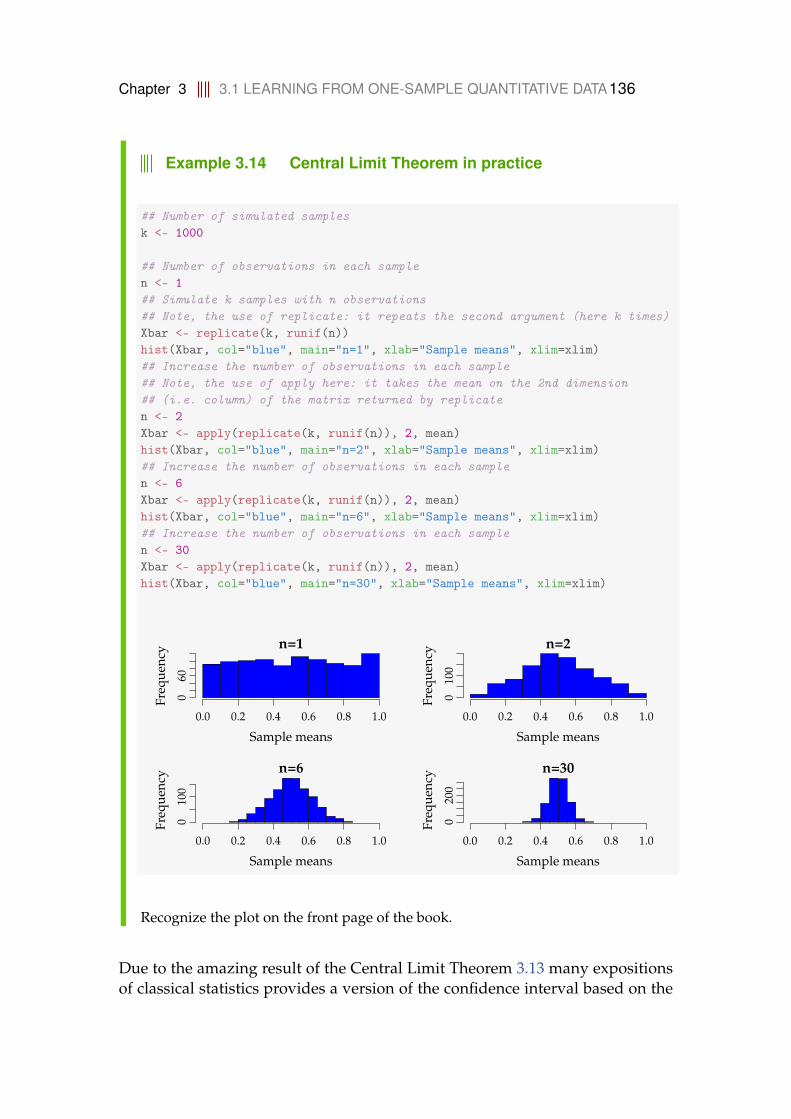
Chapter 3 3.1 LEARNING FROM ONE-SAMPLE QUANTITATIVE DATA136
Example 3.14 Central Limit Theorem in practice
## Number of simulated samplesk <- 1000
## Number of observations in each samplen <- 1## Simulate k samples with n observations## Note, the use of replicate: it repeats the second argument (here k times)Xbar <- replicate(k, runif(n))hist(Xbar, col="blue", main="n=1", xlab="Sample means", xlim=xlim)## Increase the number of observations in each sample## Note, the use of apply here: it takes the mean on the 2nd dimension## (i.e. column) of the matrix returned by replicaten <- 2Xbar <- apply(replicate(k, runif(n)), 2, mean)hist(Xbar, col="blue", main="n=2", xlab="Sample means", xlim=xlim)## Increase the number of observations in each samplen <- 6Xbar <- apply(replicate(k, runif(n)), 2, mean)hist(Xbar, col="blue", main="n=6", xlab="Sample means", xlim=xlim)## Increase the number of observations in each samplen <- 30Xbar <- apply(replicate(k, runif(n)), 2, mean)hist(Xbar, col="blue", main="n=30", xlab="Sample means", xlim=xlim)
n=1
Sample means
Freq
uenc
y
0.0 0.2 0.4 0.6 0.8 1.0
060
n=2
Sample means
Freq
uenc
y
0.0 0.2 0.4 0.6 0.8 1.0
010
0
n=6
Sample means
Freq
uenc
y
0.0 0.2 0.4 0.6 0.8 1.0
010
0
n=30
Sample means
Freq
uenc
y
0.0 0.2 0.4 0.6 0.8 1.0
020
0
Recognize the plot on the front page of the book.
Due to the amazing result of the Central Limit Theorem 3.13 many expositionsof classical statistics provides a version of the confidence interval based on the
Chapter 3 3.1 LEARNING FROM ONE-SAMPLE QUANTITATIVE DATA137
standard normal quantiles rather than the t-quantiles
x± z1−α/2 ·s√n
. (3-13)
We present it here only as an interesting limit situation of the t-based interval inMethod 3.8.
For large samples, the standard normal distribution and t-distribution are al-most the same, so in practical situations, it doesn’t matter whether the normalbased or the t-based confidence interval (CI) is used. Since the t-based intervalis also valid for small samples when a normal distribution is assumed, we rec-ommend that the t-based interval in Method 3.8 is used in all situations. Thisrecommendation also has the advantage that the R-function t.test, which pro-duces the t-based interval, can be used in all cases.
How large should the sample then be in a non-normal case to ensure the validityof the interval? No general answer can be given, but as a rule of thumb werecommend n ≥ 30.
When we have a small sample for which we cannot or will not make a nor-mality assumption, we have not yet presented a valid CI method. The classicalsolution is to use the so-called non-parametric methods. However, in the nextchapter we will present the more widely applicable simulation or re-samplingbased techniques.
3.1.5 Repeated sampling interpretation of confidence intervals
In this section we show that 95% of the 95% confidence intervals we make willcover the true value in the long run. Or, in general 100(1− α)% of the 100(1−α)% confidence intervals we make will cover the true value in the long run. Forexample, if we make 100 95% CI we cannot guarantee that exactly 95 of thesewill cover the true value, but if we repeatedly make 100 95% CIs then on average95 of them will cover the true value.
Example 3.15 Simulating many confidence intervals
To illustrate this with a simulation example, then we can generate 50 randomN(1, 12) distributed numbers and calculate the t-based CI given in Method 3.8, andthen repeated this 1000 times to see how many times the true mean µ = 1 is covered.The following code illustrates this:

Chapter 3 3.1 LEARNING FROM ONE-SAMPLE QUANTITATIVE DATA138
## Simulate 1000 samples of n=50 observations, and## calculate a CI from each samplek <- 1000ThousandCIs <- replicate(k, t.test(rnorm(n=50, mean=1, sd=1))$conf.int)## Count how often 1 is coveredsum(ThousandCIs[1,] < 1 & 1 < ThousandCIs[2,])
[1] 954
Hence in 954 of the 1000 repetitions (i.e. 95.4%) the CI covered the true value. Ifwe repeat the whole simulation over, we would obtain 1000 different samples andtherefore 1000 different CIs. Again we expect that approximately 95% of the CIs willcover the true value µ = 1.
The result that we arrived at by simulation in the previous example can also bederived mathematically. Since
T =X− µ
S/√
n∼ t(n− 1),
where t is the t-distribution with n− 1 degrees of freedom, it holds that
1− α = P(−t1−α/2 <
X− µ
S/√
n< t1−α/2
),
which we can rewrite as
= P(
X− t1−α/2S√n< µ < X + t1−α/2
S√n
).
Thus, the probability that the interval with limits
X± t1−α/2S√n
, (3-14)
covers the true value µ is exactly 1− α. One thing to note is that the only dif-ference between the interval above and the interval in Method 3.8, is that theinterval above is written with capital letters (simply indicating that it calculatedwith random variables rather than with observations).
This shows exactly that 100(1− α)% of the 100(1− α)% confidence interval wemake will contain the true value in the long run.
3.1.6 Confidence interval for the variance
In previous sections we discussed how to calculate a confidence interval for themean. In this section we discuss how to calculate a confidence interval for the
Chapter 3 3.1 LEARNING FROM ONE-SAMPLE QUANTITATIVE DATA139
variance or the standard deviation.
We will assume that the observations come from a normal distribution through-out this section, and we will not present any methods that are valid beyond thisassumption. While the methods for the sample mean in the previous sectionsare not sensitive to (minor) deviations from the normal distribution, the meth-ods discussed in this section for the sample variance rely much more heavily onthe correctness of the normal distribution assumption.
Example 3.16 Tablet production
In the production of tablets, an active matter is mixed with a powder and then themixture is formed to tablets. It is important that the mixture is homogenous, suchthat each tablet has the same strength.
We consider a mixture (of the active matter and powder) from where a large amountof tablets is to be produced.
We seek to produce the mixtures (and the final tablets) such that the mean content ofthe active matter is 1 mg/g with the smallest variance possible. A random sample iscollected where the amount of active matter is measured. It is assumed that all themeasurements follow a normal distribution.
The variance estimator, that is, the formula for the variance seen as a randomvariable, is
S2 =1
n− 1
n
∑i=1
(Xi − X)2, (3-15)
where n is the number of observations, Xi is observation number i where i =1, . . . , n, and X is the estimator of the mean of X.
The (sampling) distribution of the variance estimator is the χ2-distribution dis-tribution: let S2 be the variance of a sample of size n from a normal distributionwith variance σ2, then
χ2 =(n− 1)S2
σ2 ,
is a stochastic variable following the χ2-distribution with v = n− 1 degrees offreedom.
The χ2-distribution, as any other distribution, has a probability density func-tion. It is a non-symmetric distribution on the positive axis. It is a distributionof squared normal random variables, for more details see Section 2.10.1. Anexample of a χ2-distribution is given in the following:

Chapter 3 3.1 LEARNING FROM ONE-SAMPLE QUANTITATIVE DATA140
Example 3.17 The χ2-distribution
The density of the χ2-distribution with 9 degrees of freedom is:
## The chisquare-distribution with df=9 (the density)x <- seq(0, 35, by = 0.1)plot(x, dchisq(x, df = 9), type = "l", ylab="Density")
0 5 10 15 20 25 30 35
0.00
0.02
0.04
0.06
0.08
0.10
x
Den
sity
So, the χ2-distributions are directly available in R, via the similar four typesof R-functions as seen for the other probability distributions presented in thedistribution overview, see Appendix A.3.
Hence, we can easily work with χ2-distributions in practice. As indicated thereis a different χ2-distribution for each n.
Chapter 3 3.1 LEARNING FROM ONE-SAMPLE QUANTITATIVE DATA141
Method 3.18 Confidence interval for the variance/standard devia-tion
A 100(1− α)% confidence interval for the variance σ2 is[(n− 1)s2
χ21−α/2
,(n− 1)s2
χ2α/2
], (3-16)
where the quantiles come from a χ2-distribution with ν = n− 1 degrees offreedom.
A 100(1− α)% confidence interval for the standard deviation σ is[√
(n− 1)s2
χ21−α/2
,
√(n− 1)s2
χ2α/2
]. (3-17)
Note: The confidence intervals for the variance and standard deviations aregenerally non-symmetric as opposed to the t-based interval for the mean µ.
Example 3.19 Tablet production
A random sample of n = 20 tablets is collected and from this the mean is estimatedto x = 1.01 and the variance to s2 = 0.072. Let us find the 95%-confidence intervalfor the variance. To apply the method above we need the 0.025 and 0.975 quantilesof the χ2-distribution with ν = 20− 1 = 19 degrees of freedom
χ20.025 = 8.907, χ2
0.975 = 32.85,
which we get from R:
## Quantiles of the chi-square distribution:qchisq(p=c(0.025, 0.975), df=19)
[1] 8.907 32.852
Hence the confidence interval is[
19 · 0.072
32.85,
19 · 0.072
8.907
]≈ [0.00283, 0.0105],
and for the standard deviation the confidence interval is[√0.002834,
√0.01045
]≈ [0.053, 0.102] .

Chapter 3 3.1 LEARNING FROM ONE-SAMPLE QUANTITATIVE DATA142
3.1.7 Hypothesis testing, evidence, significance and the p-value
Example 3.20 Sleeping medicine
In a study the aim is to compare two kinds of sleeping medicine A and B. 10 testpersons tried both kinds of medicine and the following 10 DIFFERENCES betweenthe two medicine types were measured (in hours):
Person x = Beffect - Aeffect1 1.22 2.43 1.34 1.35 0.96 1.07 1.88 0.89 4.6
10 1.4
For Person 1, Medicine B provided 1.2 sleep hours more than Medicine A, etc.
Our aim is to use these data to investigate if the two treatments are different in theireffect on length of sleep. We therefore let µ represent the mean difference in sleeplength. In particular we will consider the so-called null hypothesis
H0 : µ = 0,
which states that there is no difference in sleep length between the A and B Medicines.
If the observed sample turns out to be not very likely under this null hypothesis, weconclude that the null hypothesis is unlikely to be true.
First we compute the sample mean
µ = x1 = 1.67.
As of now, we don’t know if this number is particularly small or large. If the truemean difference is zero, would it be unlikely to observe a mean difference this large?Could it be due to just random variation? To answer this question we compute theprobability of observing a sample mean that is 1.67 or further from 0 – in the casethat the true mean difference is in fact zero. This probability is called a p-value. Ifthe p-value is small (say less than 0.05), we conclude that the null hypothesis isn’ttrue. If the p-value is not small (say larger than 0.05), we conclude that we haven’tobtained sufficient evidence to falsify the null hypothesis.

Chapter 3 3.1 LEARNING FROM ONE-SAMPLE QUANTITATIVE DATA143
After some computations that you will learn to perform later in this section, weobtain a p-value
p-value ≈ 0.00117,
which indicates quite strong evidence against the null hypothesis. As a matter offact, the probability of observing a mean difference as far from zero as 1.67 or furtheris only ≈ 0.001 (one out of thousand) and therefore very small.
We conclude that the null hypothesis is unlikely to be true as it is highly incompat-ible with the observed data. We say that the observed mean µ = 1.67 is statisticallysignificantly different from zero (or simply significant implying that it is different fromzero). Or that there is a significant difference in treatment effects of B and A, and we mayconclude that Medicine B makes patients sleep significantly longer than MedicineA.
Chapter 3 3.1 LEARNING FROM ONE-SAMPLE QUANTITATIVE DATA144
p < 0.001 Very strong evidence against H00.001 ≤ p < 0.01 Strong evidence against H00.01 ≤ p < 0.05 Some evidence against H00.05 ≤ p < 0.1 Weak evidence against H0
p ≥ 0.1 Little or no evidence against H0
Table 3.1: A way to interpret the evidence for a given p-value.
The p-value
Definition 3.21 The p-value
The p-value is the probability of obtaining a test statistic that is at least asextreme as the test statistic that was actually observed. This probability iscalculated under the assumption that the null hypothesis is true.
Interpretations of a p-value:
1. The p-value measures evidence
2. The p-value measures extremeness/unusualness of the data under thenull hypothesis (“under the null hypothesis” means “assuming the nullhypothesis is true”)
The p-value is used as a general measure of evidence against a null hypothesis:the smaller the p-value, the stronger the evidence against the null hypothesisH0. A typical strength of evidence scale is given in Table 3.1.
As indicated, the definition and interpretations above are generic in the sensethat they can be used for any kind of hypothesis testing in any kind of setup.In later sections and chapters of this material, we will indeed encounter manydifferent such setups. For the specific setup in focus here, we can now give thekey method:
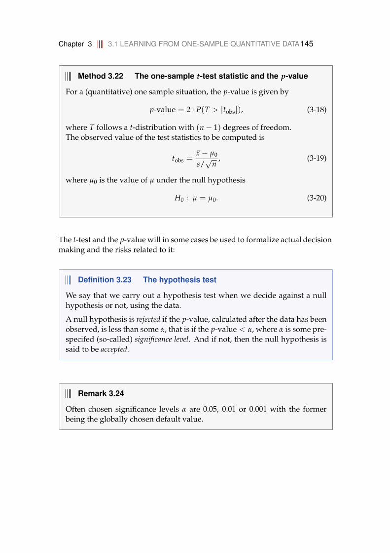
Chapter 3 3.1 LEARNING FROM ONE-SAMPLE QUANTITATIVE DATA145
Method 3.22 The one-sample t-test statistic and the p-value
For a (quantitative) one sample situation, the p-value is given by
p-value = 2 · P(T > |tobs|), (3-18)
where T follows a t-distribution with (n− 1) degrees of freedom.The observed value of the test statistics to be computed is
tobs =x− µ0
s/√
n, (3-19)
where µ0 is the value of µ under the null hypothesis
H0 : µ = µ0. (3-20)
The t-test and the p-value will in some cases be used to formalize actual decisionmaking and the risks related to it:
Definition 3.23 The hypothesis test
We say that we carry out a hypothesis test when we decide against a nullhypothesis or not, using the data.
A null hypothesis is rejected if the p-value, calculated after the data has beenobserved, is less than some α, that is if the p-value < α, where α is some pre-specifed (so-called) significance level. And if not, then the null hypothesis issaid to be accepted.
Remark 3.24
Often chosen significance levels α are 0.05, 0.01 or 0.001 with the formerbeing the globally chosen default value.

Chapter 3 3.1 LEARNING FROM ONE-SAMPLE QUANTITATIVE DATA146
Remark 3.25
A note of caution in the use of the word accepted is in place: this shouldNOT be interpreted as having proved anything: accepting a null hypothesisin statistics simply means that we could not prove it wrong! And the reasonfor this could just potentially be that we did not collect sufficient amount ofdata, and acceptance hence proofs nothing at its own right.
Example 3.26 Sleeping medicine
Continuing from Example 3.20, we now illustrate how to compute the p-value usingMethod 3.22.
## Enter sleep difference observationsx <- c(1.2, 2.4, 1.3, 1.3, 0.9, 1.0, 1.8, 0.8, 4.6, 1.4)n <- length(x)## Compute the tobs - the observed test statistictobs <- (mean(x) - 0) / (sd(x) / sqrt(n))tobs
[1] 4.672
## Compute the p-value as a tail-probability in the t-distributionpvalue <- 2 * (1-pt(abs(tobs), df=n-1))pvalue
[1] 0.001166
Naturally, as we have seen already a function in R that can do this for us
t.test(x)
One Sample t-test
data: xt = 4.7, df = 9, p-value = 0.001alternative hypothesis: true mean is not equal to 095 percent confidence interval:0.8613 2.4787
sample estimates:mean of x
1.67

Chapter 3 3.1 LEARNING FROM ONE-SAMPLE QUANTITATIVE DATA147
The confidence interval and the p-value supplements each other, and often boththe confidence interval and the p-value are reported. The confidence intervalcovers those values of the parameter that we accept given the data, while thep-value measures the extremeness of the data if the null hypothesis is true.
Example 3.27 Sleeping medicine
In the sleep medicine example the 95% confidence interval is
[0.86, 2.48] ,
so based on the data these are the values for the mean sleep difference of MedicineB versus Medicine A that we accept can be true. Only if the data is so extreme (i.e.rarely occuring) that we would only observe it 5% of the time the confidence intervaldoes not cover the true mean difference in sleep.
The p-value for the null hypothesis µ = 0 was ≈ 0.001 providing strong evidenceagainst the correctness of the null hypothesis.
If the null hypothesis was true, we would only observe this large a difference insleep medicine effect levels in around one out of a thousand times. Consequentlywe conclude that the null hypothesis is unlikely to be true and reject it.
Statistical significance
The word significance can mean importance or the extent to which something mattersin our everyday language. In statistics, however, it has a very particular mean-ing: if we say that an effect is significant, it means that the p-value is so low thatthe null hypothesis stating no effect has been rejected at some significance level α.
Definition 3.28 Significant effect
An effect is said to be (statistically) significant if the p-value is less than thesignificance level α. a
aOften, α = 0.05 is adopted.
At this point an effect would amount to a µ-value different from µ0. In othercontexts we will see later, effects can be various features of interest to us.

Chapter 3 3.1 LEARNING FROM ONE-SAMPLE QUANTITATIVE DATA148
Example 3.29 Statistical significance
Consider the follwing two situations:
1. A researcher decides on a significance level of α = 0.05 and obtains p-value =
0.023. She therefore concludes that the effect is statistically significant
2. Another researcher also adopts a significance level of α = 0.05, but obtainsp-value = 0.067. He concludes that the effect was not statistically significant
From a binary decision point of view the two researchers couldn’t disagree more.However, from a scientific and more continuous evidence quantification point ofview there is not a dramatic difference between the findings of the two researchers.
In daily statistical and/or scientific jargon the word ”statistically” will often beomitted, and when results then are communicated as significant further throughmedia or other places, it gives the risk that the distinction between the twomeanings gets lost. At first sight it may appear unimportant, but the big dif-ference is the following: sometimes a statistically significant finding can be sosmall in real size that it is of no real importance. If data collection involves verybig data sizes one may find statistically significant effects that for no practicalsituations matter much or anything at all.
The null hypothesis
The null hypothesis most often expresses the status quo or that “nothing is hap-pening”. This is what we have to believe before we perform any experimentsand observe any data. This is what we have to accept in the absense of anyevidence that the situation is otherwise. For example the null hypothesis in thesleep medicine examples states that the difference in sleep medicine effect levelis unchanged by the treatment: this is what we have to accept until we obtainevidence otherwise. In this particular example the observed data and the statis-tical theory provided such evidence and we could conclude a significant effect.
The null hypothesis has to be falsifiable. This means that it should be possible tocollect evidence against it.
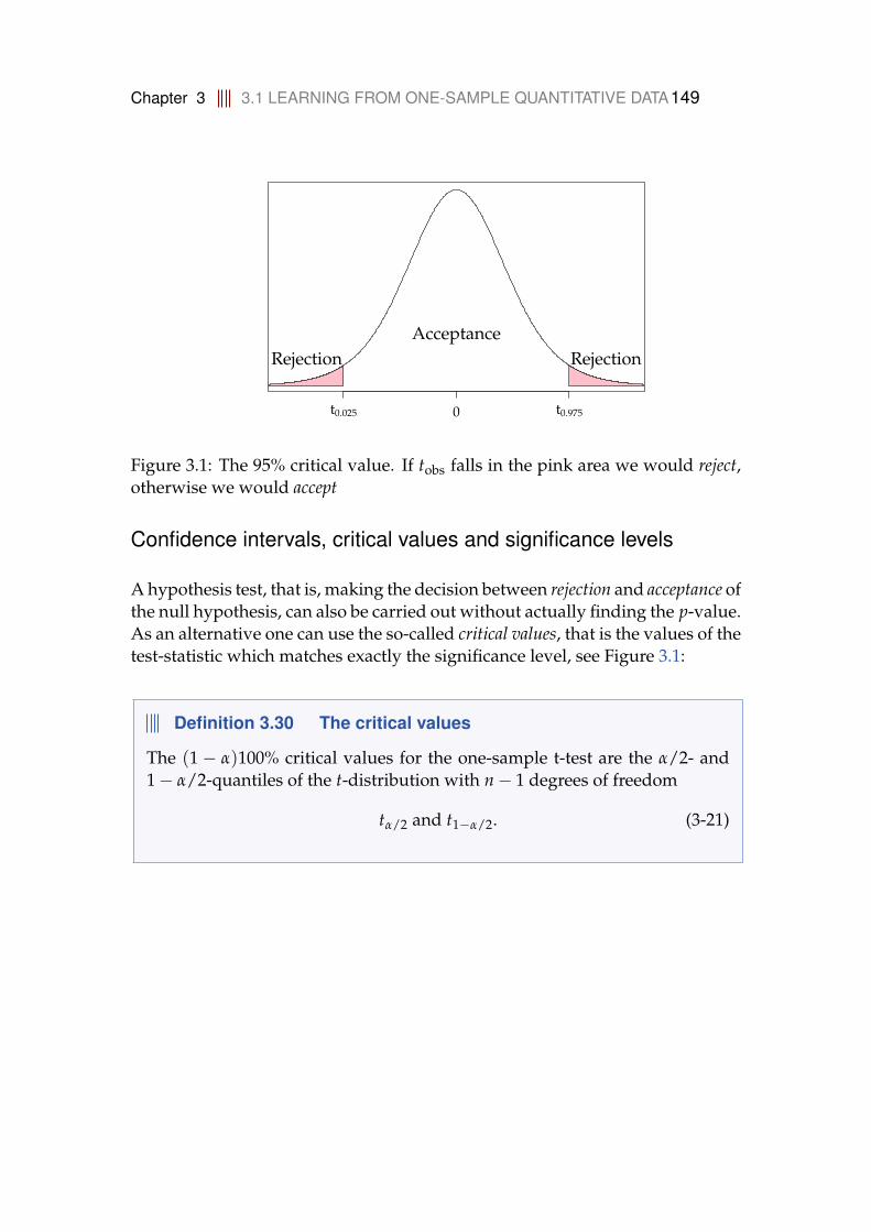
Chapter 3 3.1 LEARNING FROM ONE-SAMPLE QUANTITATIVE DATA149
AcceptanceRejection Rejection
t0.025 t0.9750
Figure 3.1: The 95% critical value. If tobs falls in the pink area we would reject,otherwise we would accept
Confidence intervals, critical values and significance levels
A hypothesis test, that is, making the decision between rejection and acceptance ofthe null hypothesis, can also be carried out without actually finding the p-value.As an alternative one can use the so-called critical values, that is the values of thetest-statistic which matches exactly the significance level, see Figure 3.1:
Definition 3.30 The critical values
The (1− α)100% critical values for the one-sample t-test are the α/2- and1− α/2-quantiles of the t-distribution with n− 1 degrees of freedom
tα/2 and t1−α/2. (3-21)
Chapter 3 3.1 LEARNING FROM ONE-SAMPLE QUANTITATIVE DATA150
Method 3.31 The one-sample hypothesis test by the critical value
A null hypothesis is rejected if the observed test-statistic is more extreme thanthe critical values
If |tobs| > t1−α/2 then reject, (3-22)
otherwise accept.
The confidence interval covers the acceptable values of the parameter given thedata:
Theorem 3.32 Confidence interval for µ
We consider a (1− α) · 100% confidence interval for µ
x± t1−α/2 ·s√n
. (3-23)
The confidence interval corresponds to the acceptance region for H0 whentesting the hypothesis
H0 : µ = µ0. (3-24)

Chapter 3 3.1 LEARNING FROM ONE-SAMPLE QUANTITATIVE DATA151
Remark 3.33
The proof of this theorem is almost straightforward: a µ0 inside the confi-dence interval will fullfill that
|x− µ0| < t1−α/2 ·s√n
, (3-25)
which is equivalent to
|x− µ0|s√n
< t1−α/2, (3-26)
and again to
|tobs| < t1−α/2, (3-27)
which then exactly states that µ0 is accepted, since the tobs is within thecritical values.
The alternative hypothesis
Some times we may in addition to the null hypothesis, also explicitly state analternative hypothesis. This completes the framework that allows us to control therates at which we make correct and wrong conclusions in light of the alternative.
The alternative hypothesis is
H1 : µ 6= µ0. (3-28)
This is sometimes called the two-sided (or non-directional) alternative hypoth-esis, because also one-sided (or directional) alternative hypothesis occur. How-ever, the one-sided setup is not included in the book apart from a small discus-sion below.
Example 3.34 Sleeping medicine – Alternative hypothesis
Continuing from Example 3.20 we can now set up the null hypothesis and the alter-native hypothesis together
H0 : µ = 0
H1 : µ 6= 0.
Chapter 3 3.1 LEARNING FROM ONE-SAMPLE QUANTITATIVE DATA152
Which means that we have exactly the same setup just formalized by adding thealternative hypothesis. The conclusion is naturally exactly the same as in before.
A generic approach for tests of hypotheses is:
1. Formulate the hypotheses and choose the level of significance α (choosethe "risk-level")
2. Calculate, using the data, the value of the test statistic
3. Calculate the p-value using the test statistic and the relevant samplingdistribution, compare the p-value and the significance level α, and finallymake a conclusionorCompare the value of the test statistic with the relevant critical value(s)and make a conclusion
Combining this generic hypothesis test approach with the specific method boxesof the previous section, we can now below give a method box for the one-sample t-test. This is hence a collection of what was presented in the previoussection:
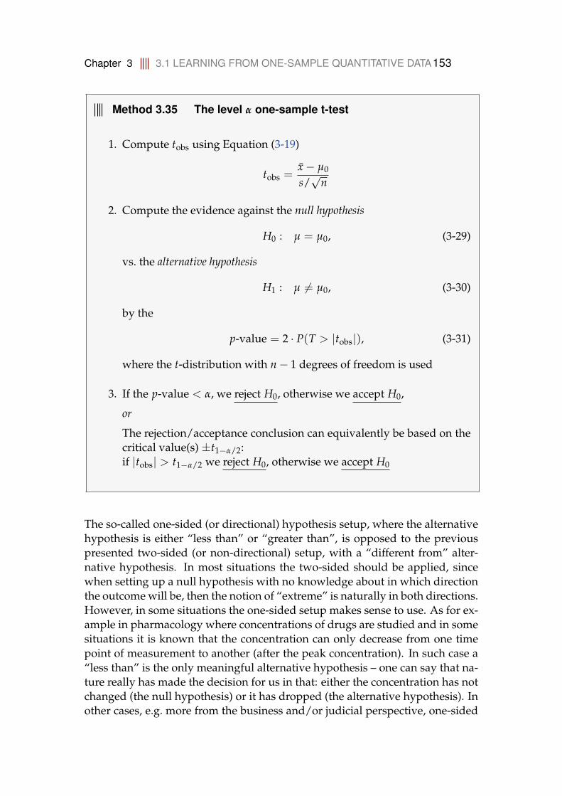
Chapter 3 3.1 LEARNING FROM ONE-SAMPLE QUANTITATIVE DATA153
Method 3.35 The level α one-sample t-test
1. Compute tobs using Equation (3-19)
tobs =x− µ0
s/√
n
2. Compute the evidence against the null hypothesis
H0 : µ = µ0, (3-29)
vs. the alternative hypothesis
H1 : µ 6= µ0, (3-30)
by the
p-value = 2 · P(T > |tobs|), (3-31)
where the t-distribution with n− 1 degrees of freedom is used
3. If the p-value < α, we reject H0, otherwise we accept H0,
or
The rejection/acceptance conclusion can equivalently be based on thecritical value(s) ±t1−α/2:if |tobs| > t1−α/2 we reject H0, otherwise we accept H0
The so-called one-sided (or directional) hypothesis setup, where the alternativehypothesis is either “less than” or “greater than”, is opposed to the previouspresented two-sided (or non-directional) setup, with a “different from” alter-native hypothesis. In most situations the two-sided should be applied, sincewhen setting up a null hypothesis with no knowledge about in which directionthe outcome will be, then the notion of “extreme” is naturally in both directions.However, in some situations the one-sided setup makes sense to use. As for ex-ample in pharmacology where concentrations of drugs are studied and in somesituations it is known that the concentration can only decrease from one timepoint of measurement to another (after the peak concentration). In such case a“less than” is the only meaningful alternative hypothesis – one can say that na-ture really has made the decision for us in that: either the concentration has notchanged (the null hypothesis) or it has dropped (the alternative hypothesis). Inother cases, e.g. more from the business and/or judicial perspective, one-sided
Chapter 3 3.1 LEARNING FROM ONE-SAMPLE QUANTITATIVE DATA154
hypothesis testing come up when for example a claim about the performance ofsome product is tested.
The one-sided “less than” hypothesis setup is: compute the evidence againstthe null hypothesis vs. the one-sided alternative hypothesis
H0 : µ ≥ µ0 (3-32)H1 : µ < µ0, (3-33)
by the
p-value = P(T < tobs). (3-34)
and equivalently for the “greather than” setup
H0 : µ ≤ µ0 (3-35)H1 : µ > µ0, (3-36)
by the
p-value = P(T > tobs). (3-37)
In both cases: if p-value < α: We reject H0, otherwise we accept H0.
Note that there are no one-sided hypothesis testing involved in the exercises.
Errors in hypothesis testing
When testing statistical hypotheses, two kind of errors can occur:
Type I: Rejection of H0 when H0 is true
Type II: Non-rejection (acceptance) of H0 when H1 is true
Example 3.36 Ambulance times
An ambulance company claims that on average it takes 20 minutes from a telephonecall to their switchboard until an ambulance reaches the location.
We might have some measurements (in minutes): 21.1, 22.3, 19.6, 24.2, ...
If our goal is to show that on average it takes longer than 20 minutes, the null- andthe alternative hypotheses are
H0 : µ = 20,
H1 : µ 6= 20.

Chapter 3 3.1 LEARNING FROM ONE-SAMPLE QUANTITATIVE DATA155
What kind of errors can occur?
Type I: Reject H0 when H0 is true, that is we mistakenly conclude that it takes longer(or shorter) than 20 minutes for the ambulance to be on location
Type II: Not reject H0 when H1 is true, that is we mistakenly conclude that it takes20 minutes for the ambulance to be on location
Example 3.37 Court of law analogy
A man is standing in a court of law accused of criminal activity.
The null- and the alternative hypotheses are
H0 : The man is not guilty,
H1 : The man is guilty.
We consider a man not guilty until evidence beyond any doubt proves him guilty.This would correspond to an α of basically zero.
Clearly, we would prefer not to do any kinds of errors, however it is a fact oflife that we cannot avoid to do so: if we would want to never do a Type I error,then we would never reject the null hypothesis, which means that we woulde.g. never conclude that one medical treatment is better than another, and thus,that we would (more) often do a Type II error, since we would never detectwhen there was a significance effect.
For the same investment (sample size n), we will increase the risk of a Type IIerror by enforcing a lower risk of a Type I error. Only by increasing n we canlower both of them, but to get both of them very low can be extremely expensiveand thus such decisions often involve economical considerations.
The statistical hypothesis testing framework is a way to formalize the handlingof the risk of the errors we may make and in this way make decisions in anenlightened way knowing what the risks are. To that end we define the twopossible risks as
P("Type I error") = α,P("Type II error") = β.
(3-38)
This notation is globally in statistical literature. The name choice for the Type Ierror is in line with the use of α for the significance level, as:
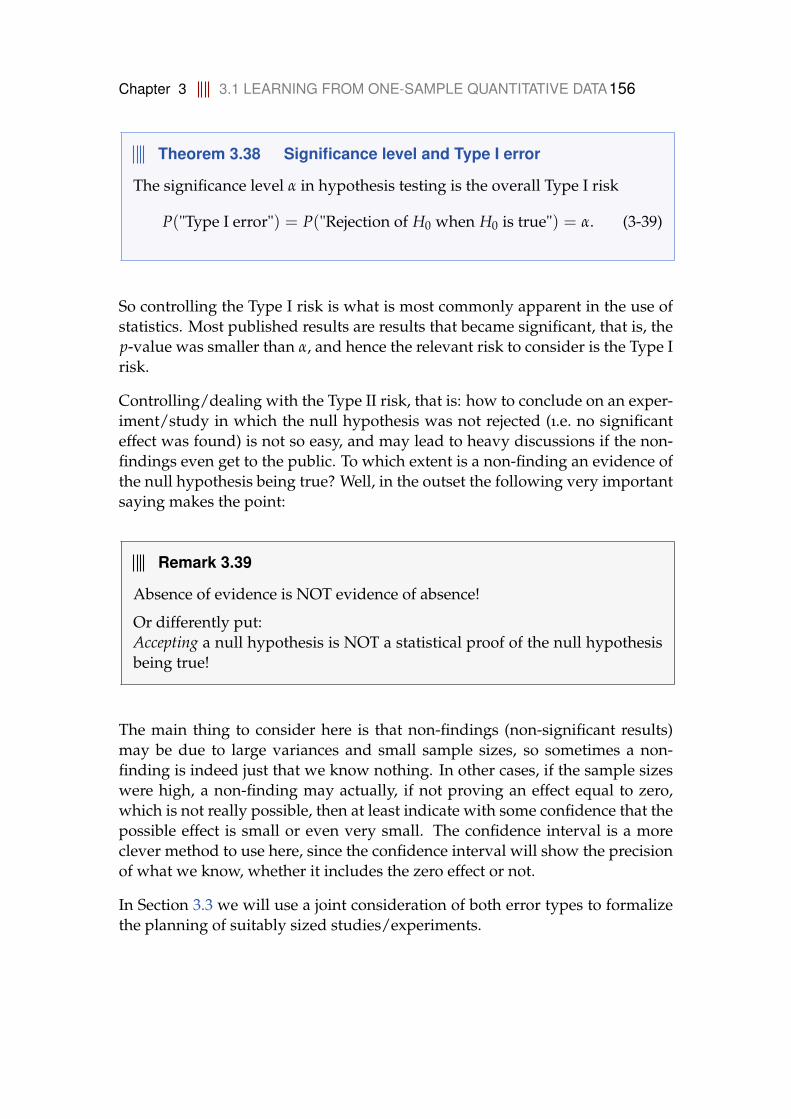
Chapter 3 3.1 LEARNING FROM ONE-SAMPLE QUANTITATIVE DATA156
Theorem 3.38 Significance level and Type I error
The significance level α in hypothesis testing is the overall Type I risk
P("Type I error") = P("Rejection of H0 when H0 is true") = α. (3-39)
So controlling the Type I risk is what is most commonly apparent in the use ofstatistics. Most published results are results that became significant, that is, thep-value was smaller than α, and hence the relevant risk to consider is the Type Irisk.
Controlling/dealing with the Type II risk, that is: how to conclude on an exper-iment/study in which the null hypothesis was not rejected (ı.e. no significanteffect was found) is not so easy, and may lead to heavy discussions if the non-findings even get to the public. To which extent is a non-finding an evidence ofthe null hypothesis being true? Well, in the outset the following very importantsaying makes the point:
Remark 3.39
Absence of evidence is NOT evidence of absence!
Or differently put:Accepting a null hypothesis is NOT a statistical proof of the null hypothesisbeing true!
The main thing to consider here is that non-findings (non-significant results)may be due to large variances and small sample sizes, so sometimes a non-finding is indeed just that we know nothing. In other cases, if the sample sizeswere high, a non-finding may actually, if not proving an effect equal to zero,which is not really possible, then at least indicate with some confidence that thepossible effect is small or even very small. The confidence interval is a moreclever method to use here, since the confidence interval will show the precisionof what we know, whether it includes the zero effect or not.
In Section 3.3 we will use a joint consideration of both error types to formalizethe planning of suitably sized studies/experiments.
Chapter 3 3.1 LEARNING FROM ONE-SAMPLE QUANTITATIVE DATA157
3.1.8 Assumptions and how to check them
The t-tests that have been presented above are based on some assumptionsabout the sampling and the population. In Theorem 3.2 the formulations arethat the random variables X1, . . . , Xn are independent and identically normallydistributed: Xi ∼ N(µ, σ2). In this statement there are two assumptions:
• Independent observations
• Normal distribution
The assumption about independent observations can be difficult to check. Itmeans that each observation must bring a unique new amount of information tothe study. Independence will be violated if some measurements are not on ran-domly selected units and share some feature – returning to the student heightexample: we do not want to include twins or families in general. Having a sam-ple of n = 20 heights, where 15 of them stem from a meeting with a large familygroup would not be 20 independent observations. The independence assump-tion is mainly checked by having information about the sampling procedure.
The assumption about normality can be checked graphically using the actualsample at hand.
Example 3.40 Student heights
We will return to the height of the ten students from example 3.1. If we want tocheck whether the sample of heights could come from a normal distribution thenwe could plot a histogram and look for a symmetric bell-shape:

Chapter 3 3.1 LEARNING FROM ONE-SAMPLE QUANTITATIVE DATA158
## The height samplex <- c(168,161,167,179,184,166,198,187,191,179)
## Using histogramspar(mfrow=c(1,3), mar=c(4,3,1,1))hist(x, xlab="Height", main="")hist(x, xlab="Height", main="", breaks=8)hist(x, xlab="Height", main="", breaks=2)
Height
Freq
uenc
y
160 180 200
01
23
4
Height
Freq
uenc
y
160 180 200
0.0
0.5
1.0
1.5
2.0
2.5
3.0
Height
Freq
uenc
y
160 180 2000
12
34
56
However, as we can see the histograms change shape depending on the number ofbreaks.
Instead of using histograms, one can plot empirical cumulative distribution (see1.6.2) and compare it with the best fitting normal distribution, in this case N(µ =
178, σ2 = 12.212):
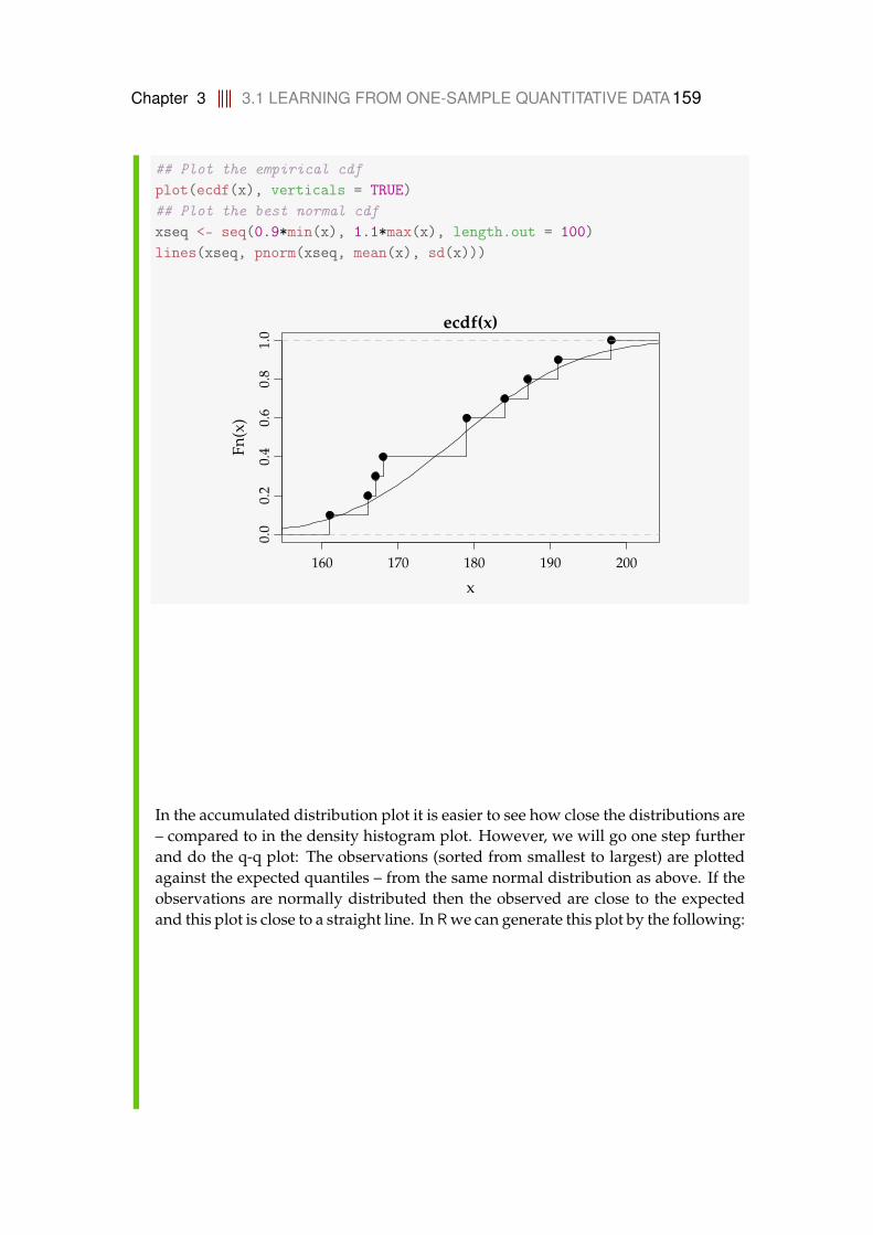
Chapter 3 3.1 LEARNING FROM ONE-SAMPLE QUANTITATIVE DATA159
## Plot the empirical cdfplot(ecdf(x), verticals = TRUE)## Plot the best normal cdfxseq <- seq(0.9*min(x), 1.1*max(x), length.out = 100)lines(xseq, pnorm(xseq, mean(x), sd(x)))
160 170 180 190 200
0.0
0.2
0.4
0.6
0.8
1.0
ecdf(x)
x
Fn(x
)
In the accumulated distribution plot it is easier to see how close the distributions are– compared to in the density histogram plot. However, we will go one step furtherand do the q-q plot: The observations (sorted from smallest to largest) are plottedagainst the expected quantiles – from the same normal distribution as above. If theobservations are normally distributed then the observed are close to the expectedand this plot is close to a straight line. In R we can generate this plot by the following:
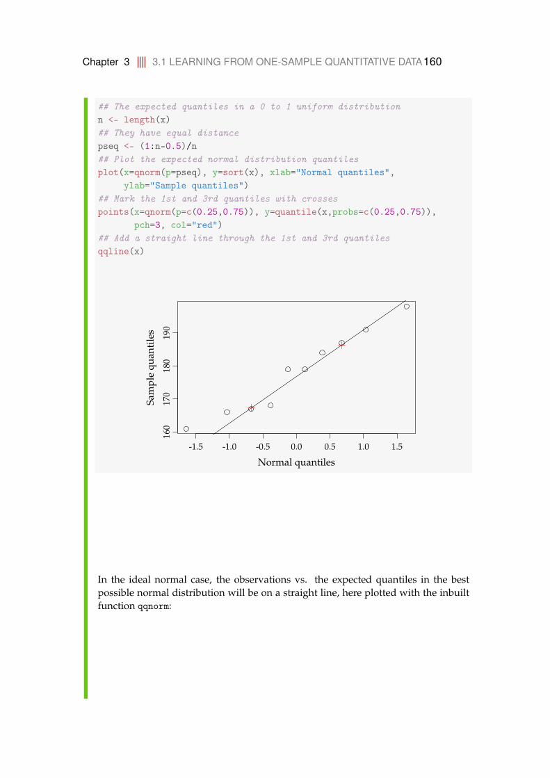
Chapter 3 3.1 LEARNING FROM ONE-SAMPLE QUANTITATIVE DATA160
## The expected quantiles in a 0 to 1 uniform distributionn <- length(x)## They have equal distancepseq <- (1:n-0.5)/n## Plot the expected normal distribution quantilesplot(x=qnorm(p=pseq), y=sort(x), xlab="Normal quantiles",
ylab="Sample quantiles")## Mark the 1st and 3rd quantiles with crossespoints(x=qnorm(p=c(0.25,0.75)), y=quantile(x,probs=c(0.25,0.75)),
pch=3, col="red")## Add a straight line through the 1st and 3rd quantilesqqline(x)
-1.5 -1.0 -0.5 0.0 0.5 1.0 1.5
160
170
180
190
Normal quantiles
Sam
ple
quan
tile
s
In the ideal normal case, the observations vs. the expected quantiles in the bestpossible normal distribution will be on a straight line, here plotted with the inbuiltfunction qqnorm:
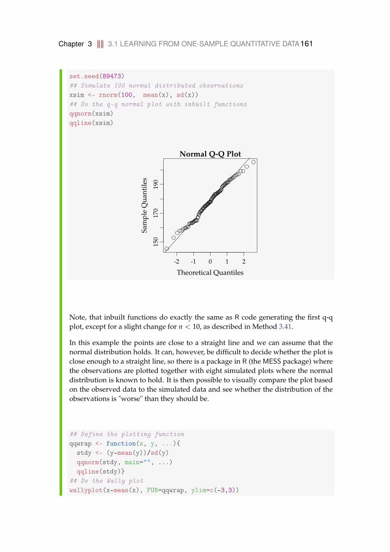
Chapter 3 3.1 LEARNING FROM ONE-SAMPLE QUANTITATIVE DATA161
set.seed(89473)## Simulate 100 normal distributed observationsxsim <- rnorm(100, mean(x), sd(x))## Do the q-q normal plot with inbuilt functionsqqnorm(xsim)qqline(xsim)
-2 -1 0 1 2
150
170
190
Normal Q-Q Plot
Theoretical Quantiles
Sam
ple
Qua
ntile
s
Note, that inbuilt functions do exactly the same as R code generating the first q-qplot, except for a slight change for n < 10, as described in Method 3.41.
In this example the points are close to a straight line and we can assume that thenormal distribution holds. It can, however, be difficult to decide whether the plot isclose enough to a straight line, so there is a package in R (the MESS package) wherethe observations are plotted together with eight simulated plots where the normaldistribution is known to hold. It is then possible to visually compare the plot basedon the observed data to the simulated data and see whether the distribution of theobservations is "worse" than they should be.
## Define the plotting functionqqwrap <- function(x, y, ...){
stdy <- (y-mean(y))/sd(y)qqnorm(stdy, main="", ...)qqline(stdy)}
## Do the Wally plotwallyplot(x-mean(x), FUN=qqwrap, ylim=c(-3,3))
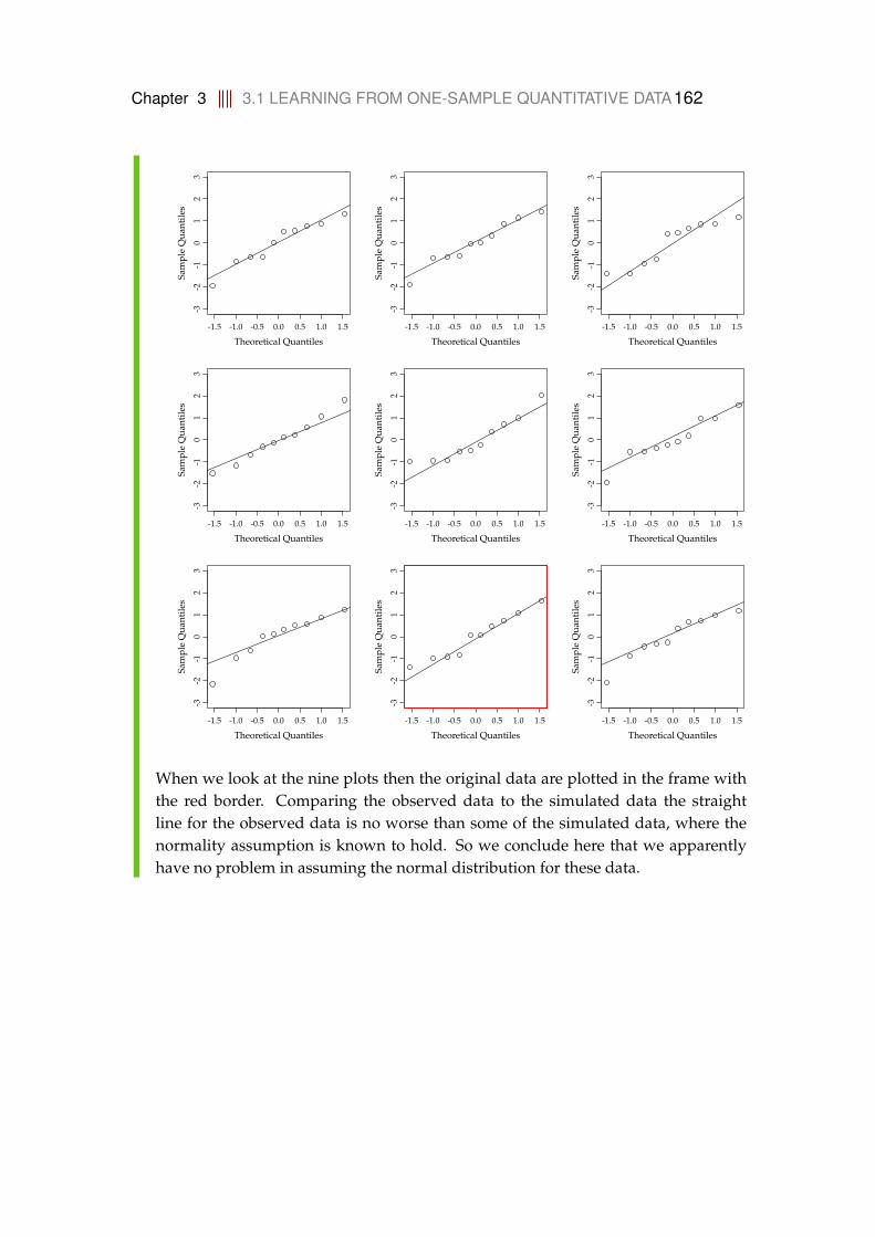
Chapter 3 3.1 LEARNING FROM ONE-SAMPLE QUANTITATIVE DATA162
-1.5 -1.0 -0.5 0.0 0.5 1.0 1.5
-3-2
-10
12
3
Theoretical Quantiles
Sam
ple
Qua
ntile
s
-1.5 -1.0 -0.5 0.0 0.5 1.0 1.5
-3-2
-10
12
3
Theoretical Quantiles
Sam
ple
Qua
ntile
s
-1.5 -1.0 -0.5 0.0 0.5 1.0 1.5
-3-2
-10
12
3
Theoretical Quantiles
Sam
ple
Qua
ntile
s
-1.5 -1.0 -0.5 0.0 0.5 1.0 1.5
-3-2
-10
12
3
Theoretical Quantiles
Sam
ple
Qua
ntile
s
-1.5 -1.0 -0.5 0.0 0.5 1.0 1.5
-3-2
-10
12
3
Theoretical Quantiles
Sam
ple
Qua
ntile
s
-1.5 -1.0 -0.5 0.0 0.5 1.0 1.5
-3-2
-10
12
3
Theoretical Quantiles
Sam
ple
Qua
ntile
s
-1.5 -1.0 -0.5 0.0 0.5 1.0 1.5
-3-2
-10
12
3
Theoretical Quantiles
Sam
ple
Qua
ntile
s
-1.5 -1.0 -0.5 0.0 0.5 1.0 1.5
-3-2
-10
12
3
Theoretical Quantiles
Sam
ple
Qua
ntile
s
-1.5 -1.0 -0.5 0.0 0.5 1.0 1.5
-3-2
-10
12
3
Theoretical Quantiles
Sam
ple
Qua
ntile
s
When we look at the nine plots then the original data are plotted in the frame withthe red border. Comparing the observed data to the simulated data the straightline for the observed data is no worse than some of the simulated data, where thenormality assumption is known to hold. So we conclude here that we apparentlyhave no problem in assuming the normal distribution for these data.
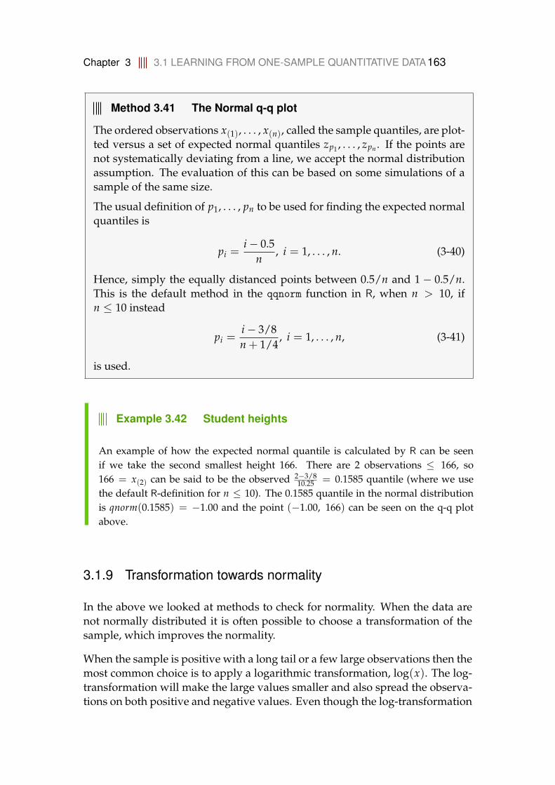
Chapter 3 3.1 LEARNING FROM ONE-SAMPLE QUANTITATIVE DATA163
Method 3.41 The Normal q-q plot
The ordered observations x(1), . . . , x(n), called the sample quantiles, are plot-ted versus a set of expected normal quantiles zp1 , . . . , zpn . If the points arenot systematically deviating from a line, we accept the normal distributionassumption. The evaluation of this can be based on some simulations of asample of the same size.
The usual definition of p1, . . . , pn to be used for finding the expected normalquantiles is
pi =i− 0.5
n, i = 1, . . . , n. (3-40)
Hence, simply the equally distanced points between 0.5/n and 1− 0.5/n.This is the default method in the qqnorm function in R, when n > 10, ifn ≤ 10 instead
pi =i− 3/8n + 1/4
, i = 1, . . . , n, (3-41)
is used.
Example 3.42 Student heights
An example of how the expected normal quantile is calculated by R can be seenif we take the second smallest height 166. There are 2 observations ≤ 166, so166 = x(2) can be said to be the observed 2−3/8
10.25 = 0.1585 quantile (where we usethe default R-definition for n ≤ 10). The 0.1585 quantile in the normal distributionis qnorm(0.1585) = −1.00 and the point (−1.00, 166) can be seen on the q-q plotabove.
3.1.9 Transformation towards normality
In the above we looked at methods to check for normality. When the data arenot normally distributed it is often possible to choose a transformation of thesample, which improves the normality.
When the sample is positive with a long tail or a few large observations then themost common choice is to apply a logarithmic transformation, log(x). The log-transformation will make the large values smaller and also spread the observa-tions on both positive and negative values. Even though the log-transformation
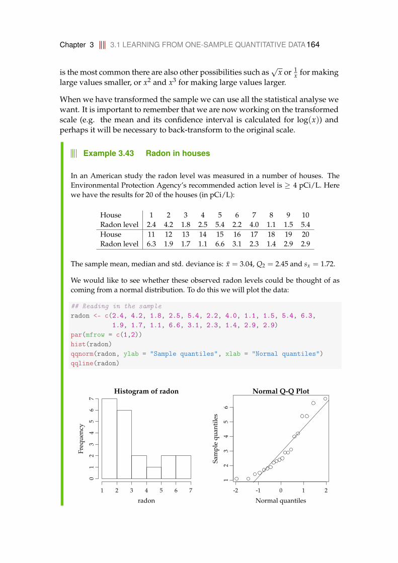
Chapter 3 3.1 LEARNING FROM ONE-SAMPLE QUANTITATIVE DATA164
is the most common there are also other possibilities such as√
x or 1x for making
large values smaller, or x2 and x3 for making large values larger.
When we have transformed the sample we can use all the statistical analyse wewant. It is important to remember that we are now working on the transformedscale (e.g. the mean and its confidence interval is calculated for log(x)) andperhaps it will be necessary to back-transform to the original scale.
Example 3.43 Radon in houses
In an American study the radon level was measured in a number of houses. TheEnvironmental Protection Agency’s recommended action level is ≥ 4 pCi/L. Herewe have the results for 20 of the houses (in pCi/L):
House 1 2 3 4 5 6 7 8 9 10Radon level 2.4 4.2 1.8 2.5 5.4 2.2 4.0 1.1 1.5 5.4House 11 12 13 14 15 16 17 18 19 20Radon level 6.3 1.9 1.7 1.1 6.6 3.1 2.3 1.4 2.9 2.9
The sample mean, median and std. deviance is: x = 3.04, Q2 = 2.45 and sx = 1.72.
We would like to see whether these observed radon levels could be thought of ascoming from a normal distribution. To do this we will plot the data:
## Reading in the sampleradon <- c(2.4, 4.2, 1.8, 2.5, 5.4, 2.2, 4.0, 1.1, 1.5, 5.4, 6.3,
1.9, 1.7, 1.1, 6.6, 3.1, 2.3, 1.4, 2.9, 2.9)par(mfrow = c(1,2))hist(radon)qqnorm(radon, ylab = "Sample quantiles", xlab = "Normal quantiles")qqline(radon)
Histogram of radon
radon
Freq
uenc
y
1 2 3 4 5 6 7
01
23
45
67
-2 -1 0 1 2
12
34
56
Normal Q-Q Plot
Normal quantiles
Sam
ple
quan
tile
s

Chapter 3 3.1 LEARNING FROM ONE-SAMPLE QUANTITATIVE DATA165
From both plots we see that the data are positive and right skewed with a few largeobservations. Therefore a log-transformation is applied:
## Transform using the natural logarithmlogRadon <- log(radon)hist(logRadon)qqnorm(logRadon, ylab = "Sample quantiles", xlab = "Normal quantiles")qqline(logRadon)
Histogram of logRadon
logRadon
Freq
uenc
y
0.0 0.5 1.0 1.5 2.0
01
23
45
67
-2 -1 0 1 2
0.5
1.0
1.5
Normal Q-Q Plot
Normal quantiles
Sam
ple
quan
tile
s
As we had expected the log-transformed data seem to be closer to a normal distri-bution.
We can now calculate the mean and 95% confidence interval for the log-transformeddata. However, we are perhaps not interested in the mean of the log-radon levels,then we have to back-transform the estimated mean and confidence interval usingexp(x). When we take the exponential of the estimated mean, then this is no longera mean but a median on the original pCi/L scale. This gives a good interpretation,as medians are useful when the distributions are not symmeric.
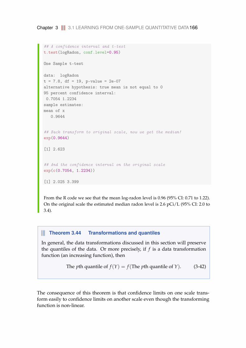
Chapter 3 3.1 LEARNING FROM ONE-SAMPLE QUANTITATIVE DATA166
## A confidence interval and t-testt.test(logRadon, conf.level=0.95)
One Sample t-test
data: logRadont = 7.8, df = 19, p-value = 2e-07alternative hypothesis: true mean is not equal to 095 percent confidence interval:0.7054 1.2234
sample estimates:mean of x
0.9644
## Back transform to original scale, now we get the median!exp(0.9644)
[1] 2.623
## And the confidence interval on the original scaleexp(c(0.7054, 1.2234))
[1] 2.025 3.399
From the R code we see that the mean log-radon level is 0.96 (95% CI: 0.71 to 1.22).On the original scale the estimated median radon level is 2.6 pCi/L (95% CI: 2.0 to3.4).
Theorem 3.44 Transformations and quantiles
In general, the data transformations discussed in this section will preservethe quantiles of the data. Or more precisely, if f is a data transformationfunction (an increasing function), then
The pth quantile of f (Y) = f (The pth quantile of Y). (3-42)
The consequence of this theorem is that confidence limits on one scale trans-form easily to confidence limits on another scale even though the transformingfunction is non-linear.
Chapter 3 3.2 LEARNING FROM TWO-SAMPLE QUANTITATIVE DATA167
3.2 Learning from two-sample quantitative data
In this section the setup, where we can learn about the difference between themeans from two populations, is presented. This is very often a setup encoun-tered in most fields of science and engineering: compare the quality of twoproducts, compare the performance of two groups, compare a new drug to aplacebo and so on. One could say, that it should be called a two-populationsetup, since it is really two populations (or groups) which are compared by tak-ing a sample from each, however it is called a two-sample setup (probably itsounds better to say).
First, the two-sample setup is introduced with an example and then methodsfor confidence intervals and tests are presented.
Example 3.45 Nutrition study
In a nutrition study the aim is to investigate if there is a difference in the energyusage for two different types of (moderately physically demanding) work. In thestudy, the energy usage of 9 nurses from hospital A and 9 (other) nurses from hos-pital B have been measured. The measurements are given in the following table inmega Joule (MJ):
Hospital A Hospital B7.53 9.217.48 11.518.08 12.798.09 11.85
10.15 9.978.40 8.79
10.88 9.696.13 9.687.90 9.19
Our aim is to assess the difference in energy usage between the two groups of nurses.If µA and µB are the mean energy expenditures for nurses from hospital A and B,then the estimates are just the sample means
µA = xA = 8.293,
µB = xB = 10.298.
To assess the difference in means, δ = µB − µA, we could consider the confidenceinterval for δ = µB − µA. Clearly, the estimate for the difference is the difference ofthe sample means, δ = µB − µA = 2.005.
Chapter 3 3.2 LEARNING FROM TWO-SAMPLE QUANTITATIVE DATA168
The 95% confidence interval is
2.005± 1.412 = [0.59, 3.42],
which spans the mean differences in energy expenditure that we find acceptablebased on the data. Thus we do not accept that the mean difference could be zero.
The interval width, given by 1.41, as we will learn below, comes from a simple com-putation using the two sample standard deviations, the two sample sizes and a t-quantile.
We can also compute a p-value to measure the evidence against the null hypothesisthat the mean energy expenditures are the same. Thus we consider the followingnull hypothesis
H0 : δ = 0.
Since the 95% confidence interval does not cover zero, we already know that the p-value for this significance test will be less than 0.05. In fact it turns out that thep-value for this significance test is 0.0083 indicating strong evidence against thenull hypothesis that the mean energy expenditures are the same for the two nursegroups. We therefore have strong evidence that the mean energy expenditure ofnurses from hospital B is higher than that of nurses from hospital A.
This section describes how to compute the confidence intervals and p-values in suchtwo-sample setups.
3.2.1 Comparing two independent means - confidence Interval
We assume now that we have a sample x1, . . . , xn taken at random from onepopulation with mean µ1 and variance σ2
1 and another sample y1, . . . , yn takenat random from another population with mean µ2 and variance σ2
2 .

Chapter 3 3.2 LEARNING FROM TWO-SAMPLE QUANTITATIVE DATA169
Method 3.46 The two-sample confidence interval for µ1 − µ2
For two samples x1, . . . , xn and y1, . . . , yn the 100(1− α)% confidence inter-val for µ1 − µ2 is given by
x− y± t1−α/2 ·√
s21
n1+
s22
n2, (3-43)
where t1−α/2 is the (1− α/2)-quantile from the t-distribution with ν degreesof freedom given from Equation (3-48)
ν =
(s2
1n1
+s2
2n2
)2
(s21/n1)2
n1−1 +(s2
2/n2)2
n2−1
. (3-44)
Note how the t-quantile used for the confidence interval is exactly what wecalled the critical value above.
Example 3.47 Nutrition study
Let us find the 95% confidence interval for µB − µA. Since the relevant t-quantile is,using ν = 15.99,
t0.975 = 2.120,
the confidence interval becomes
10.298− 8.293± 2.120 ·√
2.03949
+1.954
9,
which then gives the result as also seen above
[0.59, 3.42].
3.2.2 Comparing two independent means - hypothesis test
We describe the setup as having a random sample from each of two differentpopulations, each described by a mean and a variance:
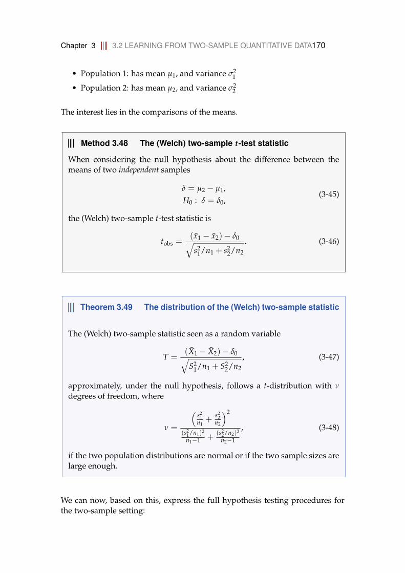
Chapter 3 3.2 LEARNING FROM TWO-SAMPLE QUANTITATIVE DATA170
• Population 1: has mean µ1, and variance σ21
• Population 2: has mean µ2, and variance σ22
The interest lies in the comparisons of the means.
Method 3.48 The (Welch) two-sample t-test statistic
When considering the null hypothesis about the difference between themeans of two independent samples
δ = µ2 − µ1,H0 : δ = δ0,
(3-45)
the (Welch) two-sample t-test statistic is
tobs =(x1 − x2)− δ0√s2
1/n1 + s22/n2
. (3-46)
Theorem 3.49 The distribution of the (Welch) two-sample statistic
The (Welch) two-sample statistic seen as a random variable
T =(X1 − X2)− δ0√
S21/n1 + S2
2/n2
, (3-47)
approximately, under the null hypothesis, follows a t-distribution with ν
degrees of freedom, where
ν =
(s2
1n1
+s2
2n2
)2
(s21/n1)2
n1−1 +(s2
2/n2)2
n2−1
, (3-48)
if the two population distributions are normal or if the two sample sizes arelarge enough.
We can now, based on this, express the full hypothesis testing procedures forthe two-sample setting:
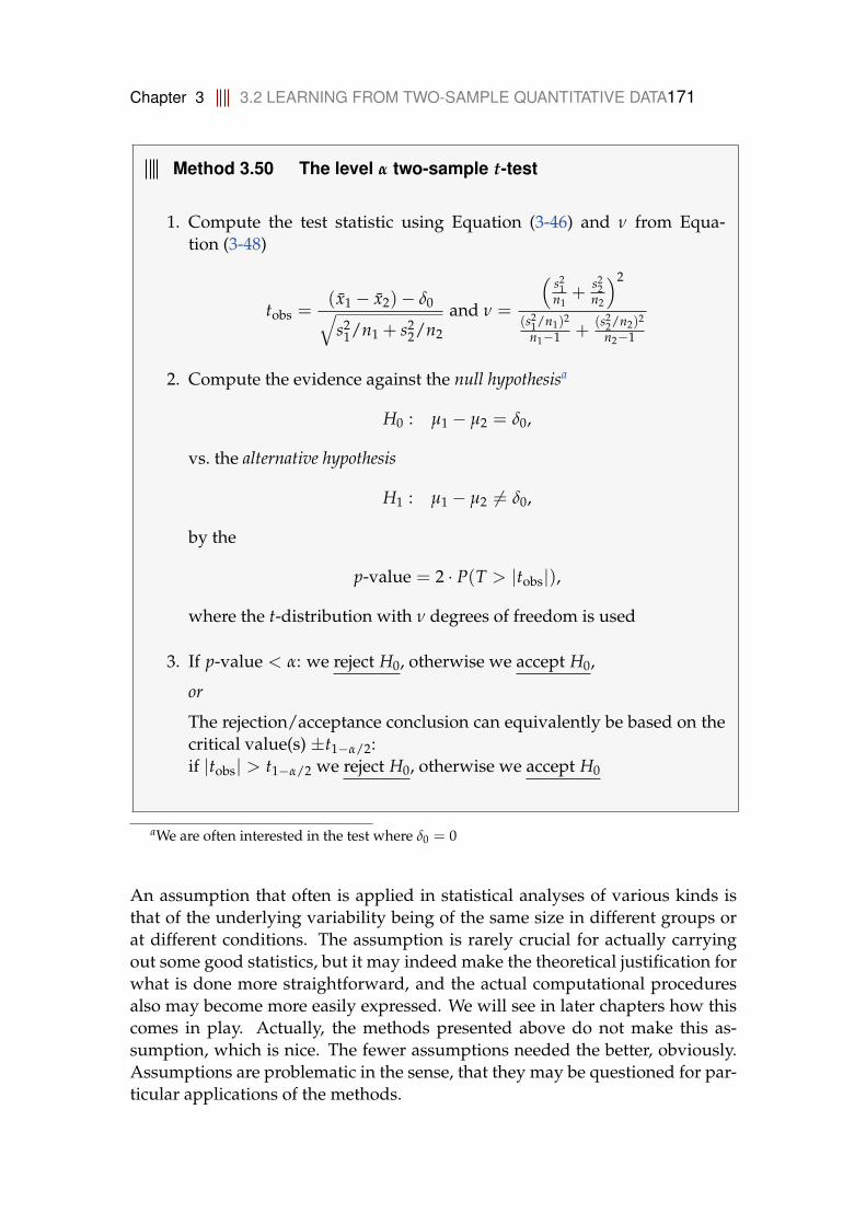
Chapter 3 3.2 LEARNING FROM TWO-SAMPLE QUANTITATIVE DATA171
Method 3.50 The level α two-sample t-test
1. Compute the test statistic using Equation (3-46) and ν from Equa-tion (3-48)
tobs =(x1 − x2)− δ0√s2
1/n1 + s22/n2
and ν =
(s2
1n1
+s2
2n2
)2
(s21/n1)2
n1−1 +(s2
2/n2)2
n2−1
2. Compute the evidence against the null hypothesisa
H0 : µ1 − µ2 = δ0,
vs. the alternative hypothesis
H1 : µ1 − µ2 6= δ0,
by the
p-value = 2 · P(T > |tobs|),
where the t-distribution with ν degrees of freedom is used
3. If p-value < α: we reject H0, otherwise we accept H0,
or
The rejection/acceptance conclusion can equivalently be based on thecritical value(s) ±t1−α/2:if |tobs| > t1−α/2 we reject H0, otherwise we accept H0
aWe are often interested in the test where δ0 = 0
An assumption that often is applied in statistical analyses of various kinds isthat of the underlying variability being of the same size in different groups orat different conditions. The assumption is rarely crucial for actually carryingout some good statistics, but it may indeed make the theoretical justification forwhat is done more straightforward, and the actual computational proceduresalso may become more easily expressed. We will see in later chapters how thiscomes in play. Actually, the methods presented above do not make this as-sumption, which is nice. The fewer assumptions needed the better, obviously.Assumptions are problematic in the sense, that they may be questioned for par-ticular applications of the methods.
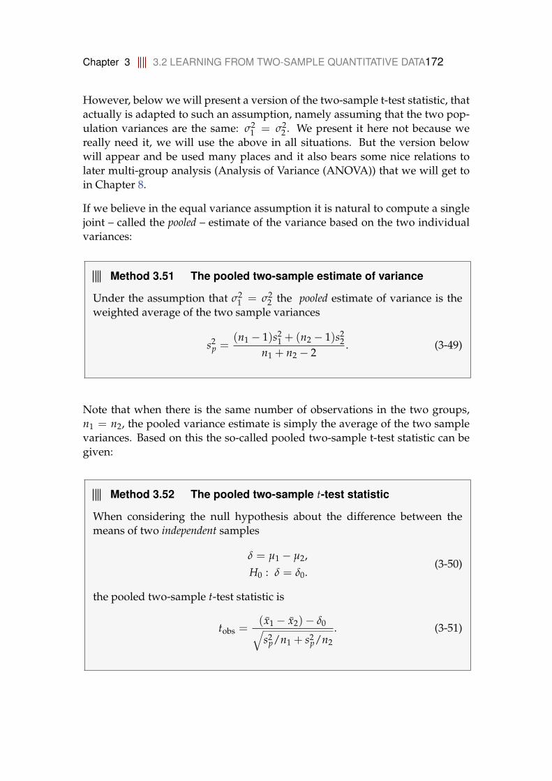
Chapter 3 3.2 LEARNING FROM TWO-SAMPLE QUANTITATIVE DATA172
However, below we will present a version of the two-sample t-test statistic, thatactually is adapted to such an assumption, namely assuming that the two pop-ulation variances are the same: σ2
1 = σ22 . We present it here not because we
really need it, we will use the above in all situations. But the version belowwill appear and be used many places and it also bears some nice relations tolater multi-group analysis (Analysis of Variance (ANOVA)) that we will get toin Chapter 8.
If we believe in the equal variance assumption it is natural to compute a singlejoint – called the pooled – estimate of the variance based on the two individualvariances:
Method 3.51 The pooled two-sample estimate of variance
Under the assumption that σ21 = σ2
2 the pooled estimate of variance is theweighted average of the two sample variances
s2p =
(n1 − 1)s21 + (n2 − 1)s2
2n1 + n2 − 2
. (3-49)
Note that when there is the same number of observations in the two groups,n1 = n2, the pooled variance estimate is simply the average of the two samplevariances. Based on this the so-called pooled two-sample t-test statistic can begiven:
Method 3.52 The pooled two-sample t-test statistic
When considering the null hypothesis about the difference between themeans of two independent samples
δ = µ1 − µ2,H0 : δ = δ0.
(3-50)
the pooled two-sample t-test statistic is
tobs =(x1 − x2)− δ0√s2
p/n1 + s2p/n2
. (3-51)
Chapter 3 3.2 LEARNING FROM TWO-SAMPLE QUANTITATIVE DATA173
And the following theorem would form the basis for hypothesis test proceduresbased on the pooled version:
Theorem 3.53 The distribution of the pooled two-sample t-teststatistic
The pooled two-sample statistic seen as a random variable:
T =(X1 − X2)− δ0√S2
p/n1 + S2p/n2
. (3-52)
follows, under the null hypothesis and under the assumption that σ21 = σ2
2 ,a t-distribution with n1 + n2 − 2 degrees of freedom if the two populationdistributions are normal.
A little consideration will show why choosing the Welch-version as the ap-proach to always use makes good sense: First of all if s2
1 = s22 the Welch and the
Pooled test statistics are the same. Only when the two variances become reallydifferent the two test-statistics may differ in any important way, and if this isthe case, we would not tend to favour the pooled version, since the assumptionof equal variances appears questionable then.
Only for cases with a small sample sizes in at least one of the two groups thepooled approach may provide slightly higher power if you believe in the equalvariance assumption. And for these cases the Welch approach is then a some-what cautious approach.
Example 3.54 Nutrition study
Let us consider the nurses example again, and test the null hypothesis expressingthat the two groups have equal means
H0 : δ = µA − µB = 0,
versus the alternative
H0 : δ = µA − µB 6= 0,
using the most commonly used significance level, α = 0.05. We follow the stepsof Method 3.50: we should first compute the test-statistic tobs and the degrees offreedom ν. These both come from the basic computations on the data:
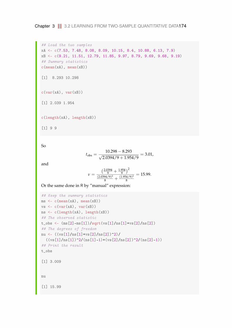
Chapter 3 3.2 LEARNING FROM TWO-SAMPLE QUANTITATIVE DATA174
## Load the two samplesxA <- c(7.53, 7.48, 8.08, 8.09, 10.15, 8.4, 10.88, 6.13, 7.9)xB <- c(9.21, 11.51, 12.79, 11.85, 9.97, 8.79, 9.69, 9.68, 9.19)## Summary statisticsc(mean(xA), mean(xB))
[1] 8.293 10.298
c(var(xA), var(xB))
[1] 2.039 1.954
c(length(xA), length(xB))
[1] 9 9
So
tobs =10.298− 8.293√
2.0394/9 + 1.954/9= 3.01,
and
ν =
( 2.03949 + 1.954
9
)2
(2.0394/9)2
8 + (1.954/9)2
8
= 15.99.
Or the same done in R by ”manual” expression:
## Keep the summary statisticsms <- c(mean(xA), mean(xB))vs <- c(var(xA), var(xB))ns <- c(length(xA), length(xB))## The observed statistict_obs <- (ms[2]-ms[1])/sqrt(vs[1]/ns[1]+vs[2]/ns[2])## The degrees of freedomnu <- ((vs[1]/ns[1]+vs[2]/ns[2])^2)/
((vs[1]/ns[1])^2/(ns[1]-1)+(vs[2]/ns[2])^2/(ns[2]-1))## Print the resultt_obs
[1] 3.009
nu
[1] 15.99
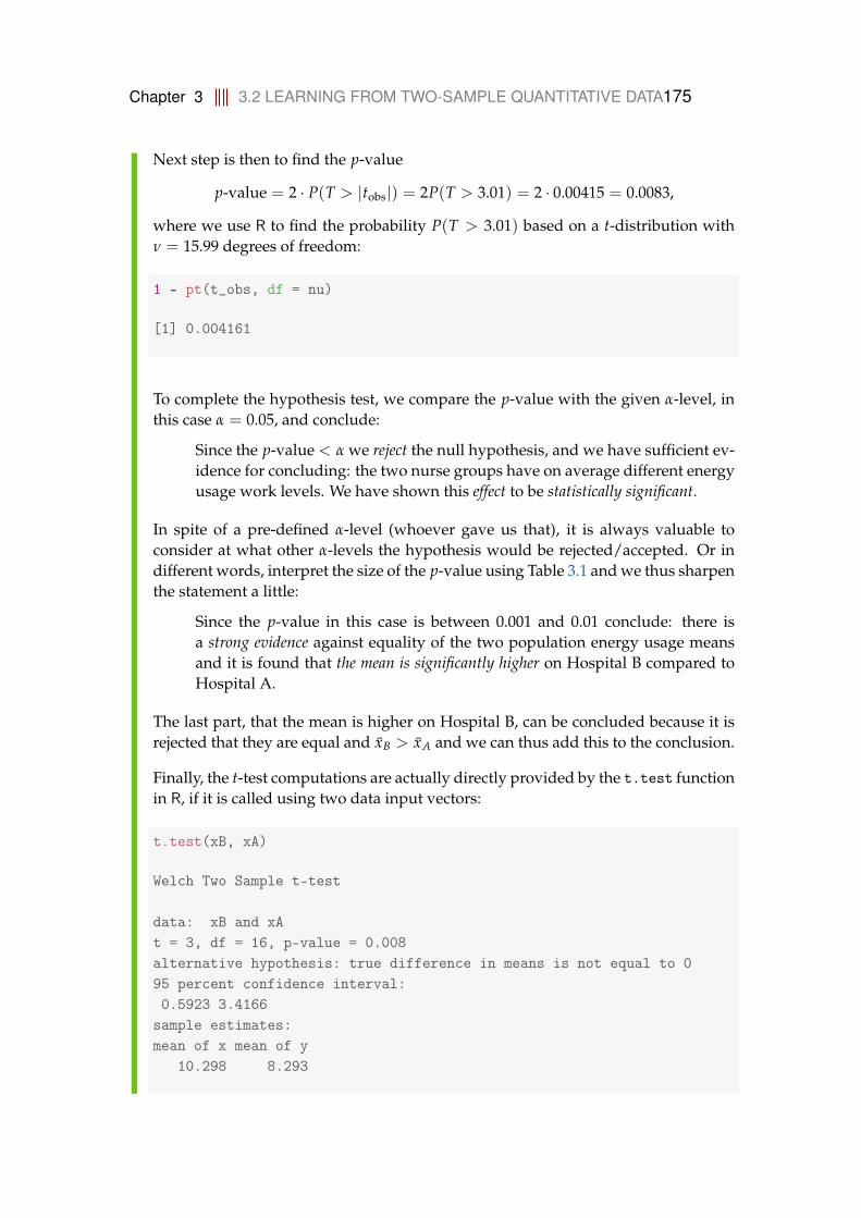
Chapter 3 3.2 LEARNING FROM TWO-SAMPLE QUANTITATIVE DATA175
Next step is then to find the p-value
p-value = 2 · P(T > |tobs|) = 2P(T > 3.01) = 2 · 0.00415 = 0.0083,
where we use R to find the probability P(T > 3.01) based on a t-distribution withν = 15.99 degrees of freedom:
1 - pt(t_obs, df = nu)
[1] 0.004161
To complete the hypothesis test, we compare the p-value with the given α-level, inthis case α = 0.05, and conclude:
Since the p-value < α we reject the null hypothesis, and we have sufficient ev-idence for concluding: the two nurse groups have on average different energyusage work levels. We have shown this effect to be statistically significant.
In spite of a pre-defined α-level (whoever gave us that), it is always valuable toconsider at what other α-levels the hypothesis would be rejected/accepted. Or indifferent words, interpret the size of the p-value using Table 3.1 and we thus sharpenthe statement a little:
Since the p-value in this case is between 0.001 and 0.01 conclude: there isa strong evidence against equality of the two population energy usage meansand it is found that the mean is significantly higher on Hospital B compared toHospital A.
The last part, that the mean is higher on Hospital B, can be concluded because it isrejected that they are equal and xB > xA and we can thus add this to the conclusion.
Finally, the t-test computations are actually directly provided by the t.test functionin R, if it is called using two data input vectors:
t.test(xB, xA)
Welch Two Sample t-test
data: xB and xAt = 3, df = 16, p-value = 0.008alternative hypothesis: true difference in means is not equal to 095 percent confidence interval:0.5923 3.4166
sample estimates:mean of x mean of y
10.298 8.293

Chapter 3 3.2 LEARNING FROM TWO-SAMPLE QUANTITATIVE DATA176
Note, how the default choices of the R-function matches our exposition:
• Default test version: the Welch (not assuming equal variances)
• Default α-level: 0.05
• Default ”direction version”: the two-sided (or non-directional) alternative hy-pothesis, see Section 3.1.7 about other alternative hypotheses)
Actually, the final rejection/acceptance conclusion based on the default (or chosen)α-level is not given by R.
In the t.test results the α-level is used for the given confidence interval for themean difference of the two populations, to be interpreted as: we accept that thetrue difference in mean energy levels between the two nurse groups is somewherebetween 0.6 and 3.4.
Remark 3.55
Often ”degrees of freedom” are integer values, but in fact t-distributionswith non-integer valued degrees of freedom are also well defined. Theν = 15.99 t-distribution (think of the density function) is a distribution inbetween the ν = 15 and the ν = 16 t-distributions. Clearly it will indeed bevery close to the ν = 16 one.
We did not in the example above use Step 4. of Method 3.50, which can becalled the critical value approach. In fact this approach is directly linked tothe confidence interval in the sense that one could make a rapid conclusionregarding rejection or not by looking at the confidence interval and checkingwhether the hypothesized value is in the interval or not. This would correspondto using the critical value approach.
Example 3.56 Nutrition study
In the nutrition example above, we can see that 0 is not in the confidence interval sowe would reject the null hypothesis. Let us formally use Step 4 of Method 3.50 tosee how this is exactly the same: the idea is that one can even before the experimentis carried out find the critical value(s), in this case:
The 5% critical values = ±t0.975 = ±2.120,
where the quantile is found from the t-distribution with ν = 15.99 degrees of free-dom:

Chapter 3 3.2 LEARNING FROM TWO-SAMPLE QUANTITATIVE DATA177
qt(0.975, df = 15.99)
[1] 2.12
Now we conclude that since the observed t-statistic tobs = 3.01 is beyond the crit-ical values (either larger than 2.120 or smaller than −2.120) the null hypothesis isrejected, and further since it was higher, that µA − µB > 0 hence µB > µA.
Example 3.57 Overlapping confidence intervals?
A commonly encountered way to visualize the results of a two-sample comparisonis to use a barplot of the means together with some measure of uncertainty, eithersimply the standard errors of the means or the 95% confidence intervals within eachgroup:
## The confidence intervals and joining the lower and upper limitsCIA <- t.test(xA)$conf.intCIB <- t.test(xB)$conf.intlower <- c(CIA[1], CIB[1])upper <- c(CIA[2], CIB[2])## First install the package with: install.packages("gplots")library(gplots)barplot2(c(mean(xA),mean(xB)), plot.ci=TRUE, ci.l=lower, ci.u=upper,
col = 2:3)
02
46
810
Here care must taken in the interpretation of this plot: it is natural, if your main
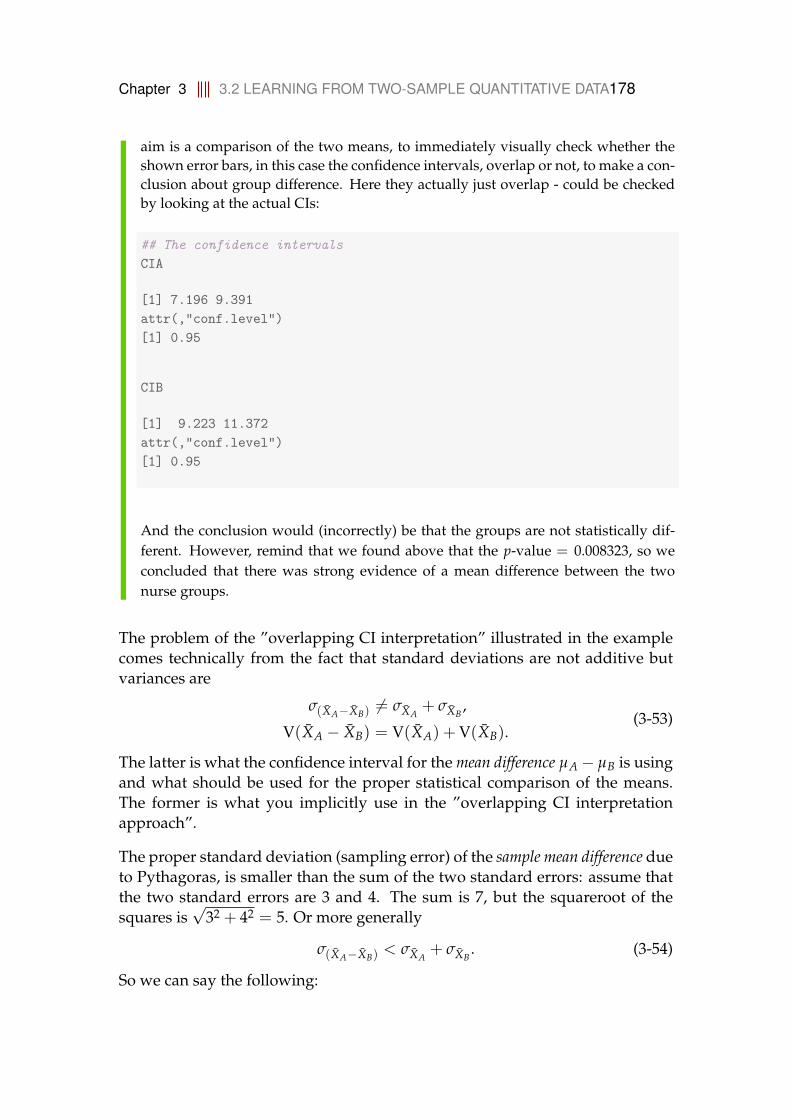
Chapter 3 3.2 LEARNING FROM TWO-SAMPLE QUANTITATIVE DATA178
aim is a comparison of the two means, to immediately visually check whether theshown error bars, in this case the confidence intervals, overlap or not, to make a con-clusion about group difference. Here they actually just overlap - could be checkedby looking at the actual CIs:
## The confidence intervalsCIA
[1] 7.196 9.391attr(,"conf.level")[1] 0.95
CIB
[1] 9.223 11.372attr(,"conf.level")[1] 0.95
And the conclusion would (incorrectly) be that the groups are not statistically dif-ferent. However, remind that we found above that the p-value = 0.008323, so weconcluded that there was strong evidence of a mean difference between the twonurse groups.
The problem of the ”overlapping CI interpretation” illustrated in the examplecomes technically from the fact that standard deviations are not additive butvariances are
σ(XA−XB)6= σXA
+ σXB,
V(XA − XB) = V(XA) + V(XB).(3-53)
The latter is what the confidence interval for the mean difference µA− µB is usingand what should be used for the proper statistical comparison of the means.The former is what you implicitly use in the ”overlapping CI interpretationapproach”.
The proper standard deviation (sampling error) of the sample mean difference dueto Pythagoras, is smaller than the sum of the two standard errors: assume thatthe two standard errors are 3 and 4. The sum is 7, but the squareroot of thesquares is
√32 + 42 = 5. Or more generally
σ(XA−XB)< σXA
+ σXB. (3-54)
So we can say the following:
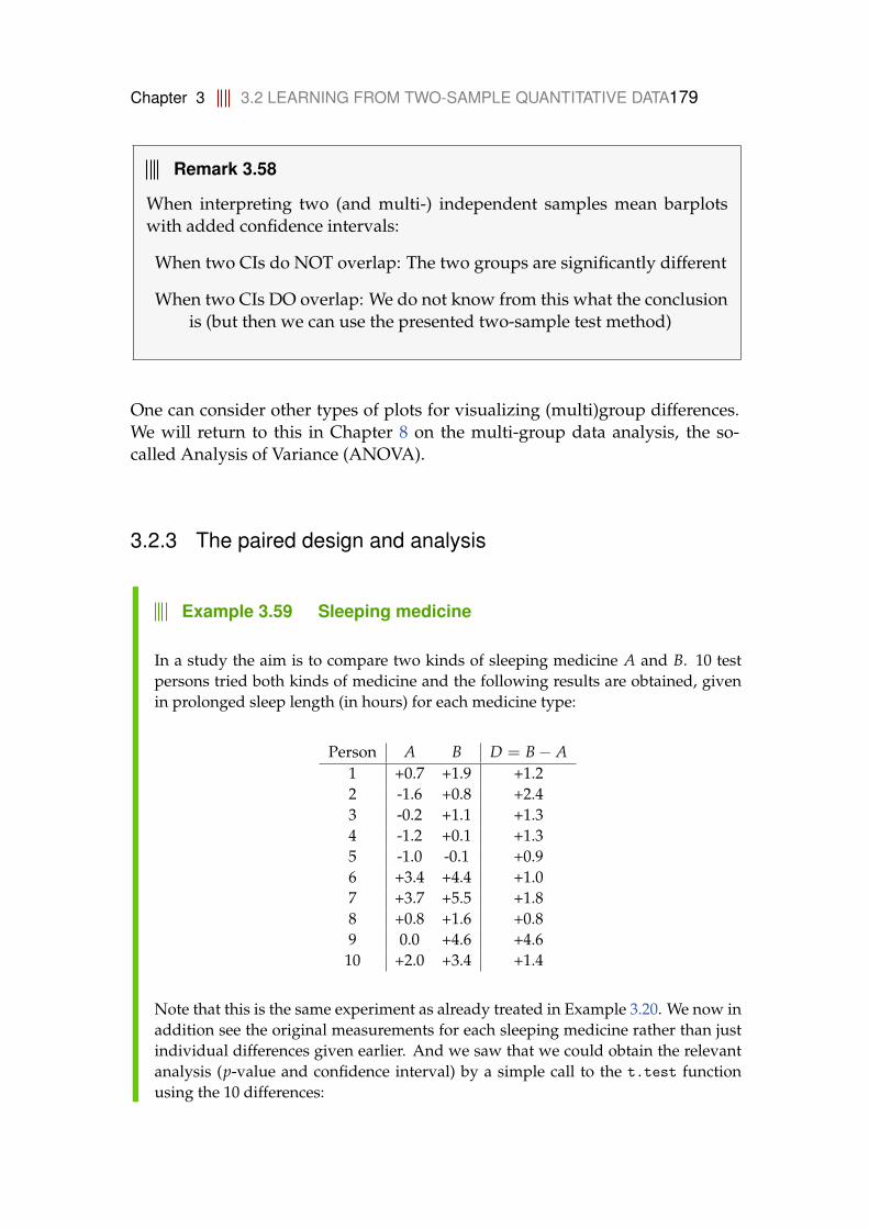
Chapter 3 3.2 LEARNING FROM TWO-SAMPLE QUANTITATIVE DATA179
Remark 3.58
When interpreting two (and multi-) independent samples mean barplotswith added confidence intervals:
When two CIs do NOT overlap: The two groups are significantly different
When two CIs DO overlap: We do not know from this what the conclusionis (but then we can use the presented two-sample test method)
One can consider other types of plots for visualizing (multi)group differences.We will return to this in Chapter 8 on the multi-group data analysis, the so-called Analysis of Variance (ANOVA).
3.2.3 The paired design and analysis
Example 3.59 Sleeping medicine
In a study the aim is to compare two kinds of sleeping medicine A and B. 10 testpersons tried both kinds of medicine and the following results are obtained, givenin prolonged sleep length (in hours) for each medicine type:
Person A B D = B− A1 +0.7 +1.9 +1.22 -1.6 +0.8 +2.43 -0.2 +1.1 +1.34 -1.2 +0.1 +1.35 -1.0 -0.1 +0.96 +3.4 +4.4 +1.07 +3.7 +5.5 +1.88 +0.8 +1.6 +0.89 0.0 +4.6 +4.610 +2.0 +3.4 +1.4
Note that this is the same experiment as already treated in Example 3.20. We now inaddition see the original measurements for each sleeping medicine rather than justindividual differences given earlier. And we saw that we could obtain the relevantanalysis (p-value and confidence interval) by a simple call to the t.test functionusing the 10 differences:
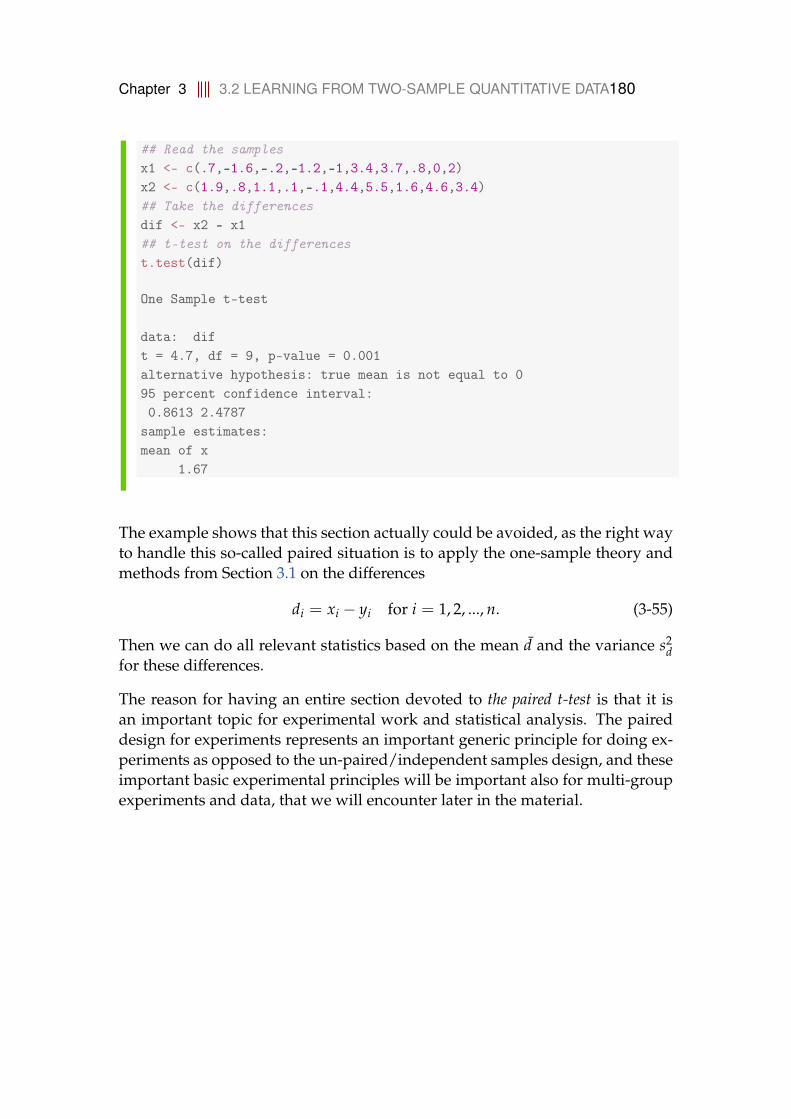
Chapter 3 3.2 LEARNING FROM TWO-SAMPLE QUANTITATIVE DATA180
## Read the samplesx1 <- c(.7,-1.6,-.2,-1.2,-1,3.4,3.7,.8,0,2)x2 <- c(1.9,.8,1.1,.1,-.1,4.4,5.5,1.6,4.6,3.4)## Take the differencesdif <- x2 - x1## t-test on the differencest.test(dif)
One Sample t-test
data: dift = 4.7, df = 9, p-value = 0.001alternative hypothesis: true mean is not equal to 095 percent confidence interval:0.8613 2.4787
sample estimates:mean of x
1.67
The example shows that this section actually could be avoided, as the right wayto handle this so-called paired situation is to apply the one-sample theory andmethods from Section 3.1 on the differences
di = xi − yi for i = 1, 2, ..., n. (3-55)
Then we can do all relevant statistics based on the mean d and the variance s2d
for these differences.
The reason for having an entire section devoted to the paired t-test is that it isan important topic for experimental work and statistical analysis. The paireddesign for experiments represents an important generic principle for doing ex-periments as opposed to the un-paired/independent samples design, and theseimportant basic experimental principles will be important also for multi-groupexperiments and data, that we will encounter later in the material.
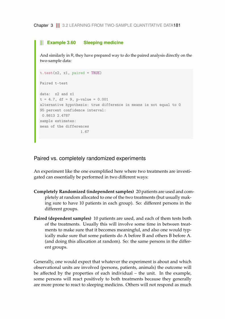
Chapter 3 3.2 LEARNING FROM TWO-SAMPLE QUANTITATIVE DATA181
Example 3.60 Sleeping medicine
And similarly in R, they have prepared way to do the paired analysis directly on thetwo-sample data:
t.test(x2, x1, paired = TRUE)
Paired t-test
data: x2 and x1t = 4.7, df = 9, p-value = 0.001alternative hypothesis: true difference in means is not equal to 095 percent confidence interval:0.8613 2.4787
sample estimates:mean of the differences
1.67
Paired vs. completely randomized experiments
An experiment like the one exemplified here where two treatments are investi-gated can essentially be performed in two different ways:
Completely Randomized (independent samples) 20 patients are used and com-pletely at random allocated to one of the two treatments (but usually mak-ing sure to have 10 patients in each group). So: different persons in thedifferent groups.
Paired (dependent samples) 10 patients are used, and each of them tests bothof the treatments. Usually this will involve some time in between treat-ments to make sure that it becomes meaningful, and also one would typ-ically make sure that some patients do A before B and others B before A.(and doing this allocation at random). So: the same persons in the differ-ent groups.
Generally, one would expect that whatever the experiment is about and whichobservational units are involved (persons, patients, animals) the outcome willbe affected by the properties of each individual – the unit. In the example,some persons will react positively to both treatments because they generallyare more prone to react to sleeping medicins. Others will not respond as much
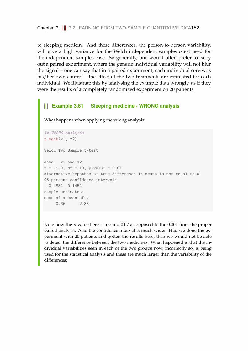
Chapter 3 3.2 LEARNING FROM TWO-SAMPLE QUANTITATIVE DATA182
to sleeping medicin. And these differences, the person-to-person variability,will give a high variance for the Welch independent samples t-test used forthe independent samples case. So generally, one would often prefer to carryout a paired experiment, where the generic individual variability will not blurthe signal – one can say that in a paired experiment, each individual serves ashis/her own control – the effect of the two treatments are estimated for eachindividual. We illustrate this by analysing the example data wrongly, as if theywere the results of a completely randomized experiment on 20 patients:
Example 3.61 Sleeping medicine - WRONG analysis
What happens when applying the wrong analysis:
## WRONG analysist.test(x1, x2)
Welch Two Sample t-test
data: x1 and x2t = -1.9, df = 18, p-value = 0.07alternative hypothesis: true difference in means is not equal to 095 percent confidence interval:-3.4854 0.1454
sample estimates:mean of x mean of y
0.66 2.33
Note how the p-value here is around 0.07 as opposed to the 0.001 from the properpaired analysis. Also the confidence interval is much wider. Had we done the ex-periment with 20 patients and gotten the results here, then we would not be ableto detect the difference between the two medicines. What happened is that the in-dividual variabilities seen in each of the two groups now, incorrectly so, is beingused for the statistical analysis and these are much larger than the variability of thedifferences:

Chapter 3 3.2 LEARNING FROM TWO-SAMPLE QUANTITATIVE DATA183
var(x1)
[1] 3.452
var(x2)
[1] 4.009
var(x1-x2)
[1] 1.278
3.2.4 Validation of assumptions with normality investigations
For normality investigations in two-sample settings we use the tools given forone-sample data, presented in Section 3.1.8. For the paired setting, the investi-gation would be carried out for the differences. For the independent case theinvestigation is carried out within each of the two groups.
Chapter 3 3.3 PLANNING A STUDY: WANTED PRECISION AND POWER184
3.3 Planning a study: wanted precision and power
Experiments and observational studies are always better when they are care-fully planned. Good planning covers many features of the study. The obser-vations must be sampled appropriately from the population, reliable measure-ments must be made and the study must be "big enough" to be able to detectan effect of interest. And if the study becomes too big, effects of little practicalinterest may become statistically significant, and (some of) the money investedin the study will be wasted. Sample size is important for economic reasons: anoversized study uses more resourses than necessary, this could be both finan-cial but also ethical if subjecting objects to potentially harmful treatments, anundersized study can be wasted if it is not able to produce reliable results.
Sample size is very important to consider before a study is carried out.
3.3.1 Sample Size for wanted precision
One way of calculating the required sample size is to work back from the wantedprecision. From (3-9) we see that the confidence interval is symmetric aroundx and the half width of the confidence interval (also called the margin of error(ME)) is given as
ME = t1−α/2σ√n
. (3-56)
Here t1−α/2 is the (1− α/2) quantile from the t-distribution with n− 1 degreesof freedom. This quantile depends on both α and the sample size n, which iswhat we want to find.
The sample size now affects both n and t1−α/2, but if we have a large sample(e.g. n ≥ 30) then we can use the normal approximation and replace t1−α/2 bythe quantile from the normal distribution z1−α/2.
In the expression for ME in Equation (3-56) we also need σ, the standard devi-ation. An estimate of the standard deviation would usually only be availableafter the sample has been taken. Instead we use a guess for σ possibly based ona pilot study or from the literature, or we could use a scenario based choice (i.e.set σ to some value which we think is reasonable).
For a given choice of ME it is now possible to isolate n in Equation (3-56) (withthe normal quantile inserted instead of the t-quantile):
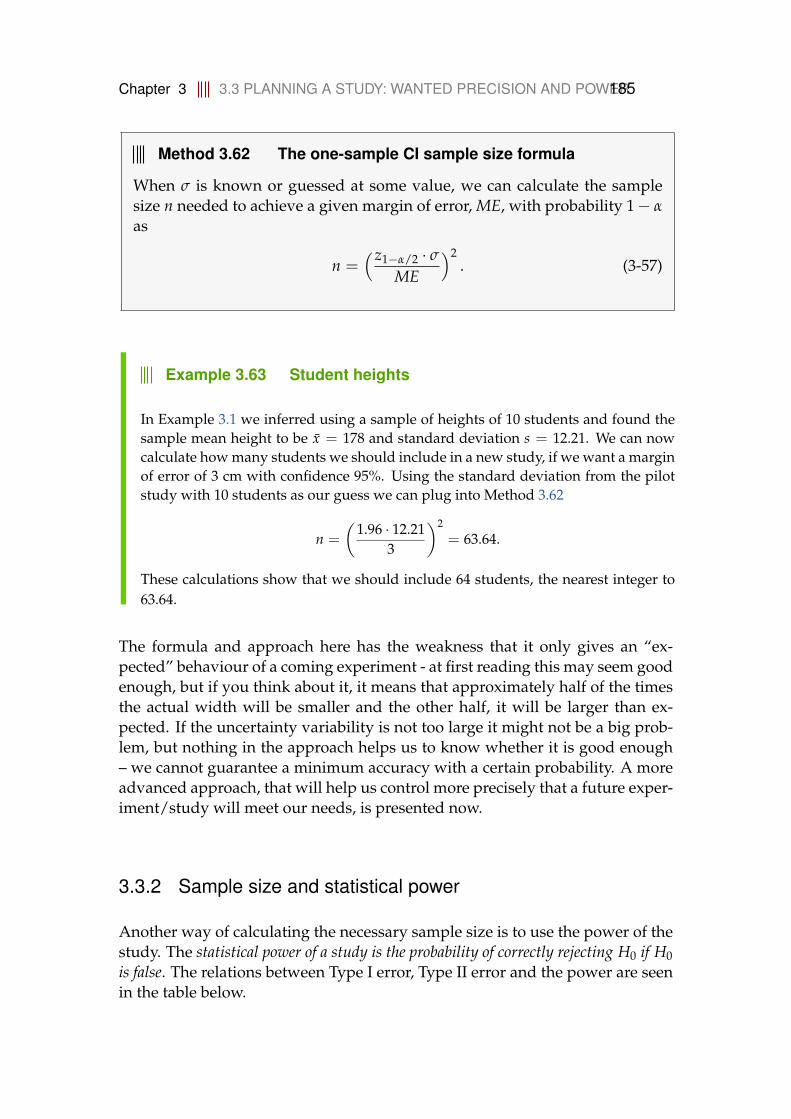
Chapter 3 3.3 PLANNING A STUDY: WANTED PRECISION AND POWER185
Method 3.62 The one-sample CI sample size formula
When σ is known or guessed at some value, we can calculate the samplesize n needed to achieve a given margin of error, ME, with probability 1− α
as
n =(z1−α/2 · σ
ME
)2. (3-57)
Example 3.63 Student heights
In Example 3.1 we inferred using a sample of heights of 10 students and found thesample mean height to be x = 178 and standard deviation s = 12.21. We can nowcalculate how many students we should include in a new study, if we want a marginof error of 3 cm with confidence 95%. Using the standard deviation from the pilotstudy with 10 students as our guess we can plug into Method 3.62
n =
(1.96 · 12.21
3
)2
= 63.64.
These calculations show that we should include 64 students, the nearest integer to63.64.
The formula and approach here has the weakness that it only gives an “ex-pected” behaviour of a coming experiment - at first reading this may seem goodenough, but if you think about it, it means that approximately half of the timesthe actual width will be smaller and the other half, it will be larger than ex-pected. If the uncertainty variability is not too large it might not be a big prob-lem, but nothing in the approach helps us to know whether it is good enough– we cannot guarantee a minimum accuracy with a certain probability. A moreadvanced approach, that will help us control more precisely that a future exper-iment/study will meet our needs, is presented now.
3.3.2 Sample size and statistical power
Another way of calculating the necessary sample size is to use the power of thestudy. The statistical power of a study is the probability of correctly rejecting H0 if H0is false. The relations between Type I error, Type II error and the power are seenin the table below.
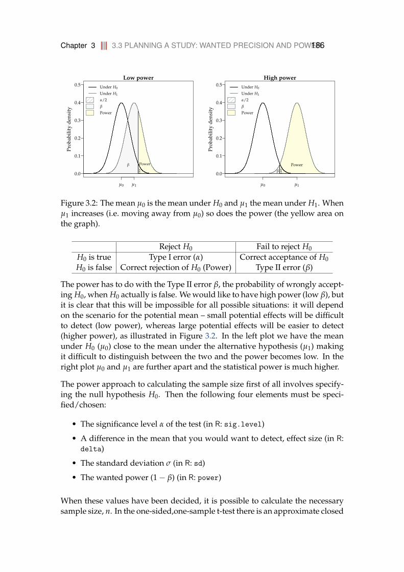
Chapter 3 3.3 PLANNING A STUDY: WANTED PRECISION AND POWER186
Low power
Prob
abili
tyde
nsit
y
µ0 µ1
0.0
0.1
0.2
0.3
0.4
0.5
α2
β Power
Under H0
Under H1
α/2
β
Power
High power
Prob
abili
tyde
nsit
y
µ0 µ1
0.0
0.1
0.2
0.3
0.4
0.5
α2β
Power
Under H0
Under H1
α/2
β
Power
Figure 3.2: The mean µ0 is the mean under H0 and µ1 the mean under H1. Whenµ1 increases (i.e. moving away from µ0) so does the power (the yellow area onthe graph).
Reject H0 Fail to reject H0H0 is true Type I error (α) Correct acceptance of H0H0 is false Correct rejection of H0 (Power) Type II error (β)
The power has to do with the Type II error β, the probability of wrongly accept-ing H0, when H0 actually is false. We would like to have high power (low β), butit is clear that this will be impossible for all possible situations: it will dependon the scenario for the potential mean – small potential effects will be difficultto detect (low power), whereas large potential effects will be easier to detect(higher power), as illustrated in Figure 3.2. In the left plot we have the meanunder H0 (µ0) close to the mean under the alternative hypothesis (µ1) makingit difficult to distinguish between the two and the power becomes low. In theright plot µ0 and µ1 are further apart and the statistical power is much higher.
The power approach to calculating the sample size first of all involves specify-ing the null hypothesis H0. Then the following four elements must be speci-fied/chosen:
• The significance level α of the test (in R: sig.level)
• A difference in the mean that you would want to detect, effect size (in R:delta)
• The standard deviation σ (in R: sd)
• The wanted power (1− β) (in R: power)
When these values have been decided, it is possible to calculate the necessarysample size, n. In the one-sided,one-sample t-test there is an approximate closed

Chapter 3 3.3 PLANNING A STUDY: WANTED PRECISION AND POWER187
form for n and this is also the case in some other simple situations. R offerseasy to use functions for this not based on the approximate normal distributionassumption, but using the more proper t-distributions. In more complicatedsettings even it is possible to do some simulations to find the required samplesize.
Method 3.64 The one-sample sample size formula
For the one-sample t-test for given α, β and σ
n =
(σ
z1−β + z1−α/2
(µ0 − µ1)
)2
,
where µ0 − µ1 is the difference in means that we would want to detect andz1−β, z1−α/2 are quantiles of the standard normal distribution.
Example 3.65 Sample size as function of power
The following figure shows how the sample size increases with increasing powerusing the formula in 3.64. Here we have chosen σ = 1 and α = 0.05. Delta isµ0 − µ1.
0.70 0.75 0.80 0.85 0.90
0
10
20
30
40
50
Power
Sam
ple
size
Delta = 0.5Delta = 0.75Delta = 1
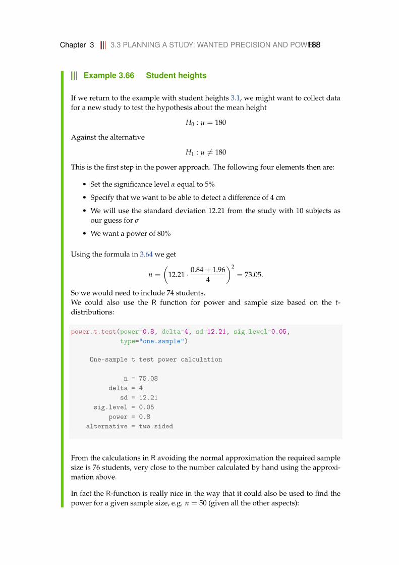
Chapter 3 3.3 PLANNING A STUDY: WANTED PRECISION AND POWER188
Example 3.66 Student heights
If we return to the example with student heights 3.1, we might want to collect datafor a new study to test the hypothesis about the mean height
H0 : µ = 180
Against the alternative
H1 : µ 6= 180
This is the first step in the power approach. The following four elements then are:
• Set the significance level α equal to 5%
• Specify that we want to be able to detect a difference of 4 cm
• We will use the standard deviation 12.21 from the study with 10 subjects asour guess for σ
• We want a power of 80%
Using the formula in 3.64 we get
n =
(12.21 · 0.84 + 1.96
4
)2
= 73.05.
So we would need to include 74 students.We could also use the R function for power and sample size based on the t-distributions:
power.t.test(power=0.8, delta=4, sd=12.21, sig.level=0.05,type="one.sample")
One-sample t test power calculation
n = 75.08delta = 4
sd = 12.21sig.level = 0.05
power = 0.8alternative = two.sided
From the calculations in R avoiding the normal approximation the required samplesize is 76 students, very close to the number calculated by hand using the approxi-mation above.
In fact the R-function is really nice in the way that it could also be used to find thepower for a given sample size, e.g. n = 50 (given all the other aspects):

Chapter 3 3.3 PLANNING A STUDY: WANTED PRECISION AND POWER189
power.t.test(n=50, delta=4, sd=12.21, sig.level=0.05,type="one.sample")
One-sample t test power calculation
n = 50delta = 4
sd = 12.21sig.level = 0.05
power = 0.6221alternative = two.sided
This would only give the power 0.62 usually considered too low for a relevant effectsize.
And finally the R-function can tell us what effect size that could be detected by, say,n = 50, and a power of 0.80:
power.t.test(n=50, power=0.80, sd=12.21, sig.level=0.05,type="one.sample")
One-sample t test power calculation
n = 50delta = 4.935
sd = 12.21sig.level = 0.05
power = 0.8alternative = two.sided
So with n = 50 only an effect size as big as 4.9 would be detectable with probability0.80.
To summarize: if we know/define 4 out the 5 values: α, 1− β, effect size, σ andn, we can find the 5’th. And to repeat, in the R-function these values are calledsig.level, power, delta, sd and n.
In the practical planning of a study, often a number of scenario-based values ofeffect size and σ are used to find a reasonable size of the study.

Chapter 3 3.3 PLANNING A STUDY: WANTED PRECISION AND POWER190
3.3.3 Power/Sample size in two-sample setup
For power and sample size one can generalize the tools presented for the one-sample setup in the previous section. We illustrate it here by an example of howto work with the inbuilt R-function:
Example 3.67 Two-sample power and sample size computationsin R
We consider the two-sample hypothesis test
H0 : µ1 = µ2,
H1 : µ1 6= µ2
## Finding the power of detecting a group difference of 2## with sigma=1 for n=10power.t.test(n=10, delta=2, sd=1, sig.level=0.05)
Two-sample t test power calculation
n = 10delta = 2
sd = 1sig.level = 0.05
power = 0.9882alternative = two.sided
NOTE: n is number in *each* group
## Finding the sample size for detecting a group difference of 2## with sigma=1 and power=0.9power.t.test(power=0.90, delta=2, sd=1, sig.level=0.05)
Two-sample t test power calculation
n = 6.387delta = 2
sd = 1sig.level = 0.05
power = 0.9alternative = two.sided
NOTE: n is number in *each* group

Chapter 3 3.3 PLANNING A STUDY: WANTED PRECISION AND POWER191
## Finding the detectable effect size (delta)## with sigma=1, n=10 and power=0.9power.t.test(power=0.90, n=10, sd=1, sig.level=0.05)
Two-sample t test power calculation
n = 10delta = 1.534
sd = 1sig.level = 0.05
power = 0.9alternative = two.sided
NOTE: n is number in *each* group
Note how the two-sample t-test is the default choice of the R-function. Previously,when we used the same function for the one-sample tests, we used the optionstype="one.sample".
Chapter 3 3.4 EXERCISES 192
3.4 Exercises
Exercise 3.1 Concrete items
A construction company receives concrete items for a construction. The lengthof the items are assumed reasonably normally distributed. The following re-quirements for the length of the elements are made
µ = 3000 mm.
The company samples 9 items from a delevery which are then measured forcontrol. The following measurements (in mm) are found:
3003 3005 2997 3006 2999 2998 3007 3005 3001
a) Compute the following three statistics: the sample mean, the sample stan-dard deviation and the standard error of the mean, and what are the in-terpretations of these statistics?
b) In a construction process, 5 concrete items are joined together to a singleconstruction with a length which is then the complete length of the 5 con-crete items. It is very important that the length of this new constructionis within 15 m plus/minus 1 cm. How often will it happen that such aconstruction will be more than 1 cm away from the 15 m target (assumethat the population mean concrete item length is µ = 3000 mm and thatthe population standard deviation is σ = 3)?
c) Find the 95% confidence interval for the mean µ.
d) Find the 99% confidence interval for µ. Compare with the 95% one fromabove and explain why it is smaller/larger!

Chapter 3 3.4 EXERCISES 193
e) Find the 95% confidence intervals for the variance σ2 and the standarddeviation σ.
f) Find the 99% confidence intervals for the variance σ2 and the standarddeviation σ.
Exercise 3.2 Aluminum profile
The length of an aluminum profile is checked by taking a sample of 16 itemswhose length is measured. The measurement results from this sample are listedbelow, all measurements are in mm:
180.02 180.00 180.01 179.97 179.92 180.05 179.94 180.10180.24 180.12 180.13 180.22 179.96 180.10 179.96 180.06
From data is obtained: x = 180.05 and s = 0.0959.
It can be assumed that the sample comes from a population which is normaldistributed.
a) A 90%-confidence interval for µ becomes?
b) A 99%-confidence interval for σ becomes?
Exercise 3.3 Concrete items (hypothesis testing)
This is a continuation of Exercise 1, so the same setting and data is used (readthe initial text of it).
a) To investigate whether the requirement to the mean is fulfilled (with α =5%), the following hypothesis should be tested
H0 : µ = 3000H1 : µ 6= 3000.
Or similarly asked: what is the evidence against the null hypothesis?

Chapter 3 3.4 EXERCISES 194
b) What would the level α = 0.01 critical values be for this test, and what arethe interpretation of these?
c) What would the level α = 0.05 critical values be for this test (compare alsowith the values found in the previous question)?
d) Investigate, by som plots, whether the data here appears to be comingfrom a normal distribution (as assumed until now)?
e) Assuming that you, maybe among different plots, also did the normal q-qplot above, the question is now: What exactly is plotted in that plot? Ormore specifically: what are the x- and y-coordinates of e.g. the two pointsto the lower left in this plot?
Exercise 3.4 Aluminium profile (hypothesis testing)
We use the same setting and data as in Exercise 2, so read the initial text of it.
a) Find the evidence against the following hypothesis:
H0 : µ = 180.
b) If the following hypothesis test is carried out
H0 : µ = 180,H1 : µ 6= 180.
What are the level α = 1% critical values for this test?
Chapter 3 3.4 EXERCISES 195
c) What is the 99%-confidence interval for µ?
d) Carry out the following hypothesis test
H0 : µ = 180,H1 : µ 6= 180,
using α = 5%.
Exercise 3.5 Transport times
A company, MM, selling items online wants to compare the transport times fortwo transport firms for delivery of the goods. To compare the two companiesrecordings of delivery times on a specific route were made, with a sample sizeof n = 9 for each firm. The following data were found:
Firm A: yA = 1.93 d and sA = 0.45 d,Firm B: yB = 1.49 d and sB = 0.58 d.
note that d is the SI unit for days. It is assumed that data can be regarded asstemming from normal distributions.
a) We want to test the following hypothesis
H0 : µA = µBH1 : µA 6= µB
What is the p-value, interpretation and conclusion for this test (at α = 5%level)?
b) Find the 95% confidence interval for the mean difference µA − µB.

Chapter 3 3.4 EXERCISES 196
c) What is the power of a study with n = 9 observations in each of the twosamples of detecting a potential mean difference of 0.4 between the firms(assume that σ = 0.5 and that we use α = 0.05)?
d) What effect size (mean difference) could be detected with n = 9 observa-tions in each of the two samples with a power of 0.8 (assume that σ = 0.5and that we use α = 0.05)?
e) How large a sample size (from each firm) would be needed in a new inves-tigation, if we want to detect a potential mean difference of 0.4 between thefirms with probability 0.90, that is with power=0.90 (assume that σ = 0.5and that we use α = 0.05)?
Exercise 3.6 Cholesterol
In a clinical trial of a cholesterol-lowering agent, 15 patients’ cholesterol (inmmol/L) has been measured before treatment and 3 weeks after starting treat-ment. Data are listed in the following table:
Patient 1 2 3 4 5 6 7 8 9 10 11 12 13 14 15Before 9.1 8.0 7.7 10.0 9.6 7.9 9.0 7.1 8.3 9.6 8.2 9.2 7.3 8.5 9.5After 8.2 6.4 6.6 8.5 8.0 5.8 7.8 7.2 6.7 9.8 7.1 7.7 6.0 6.6 8.4
The following is run in R:
x1 <- c(9.1, 8.0, 7.7, 10.0, 9.6, 7.9, 9.0, 7.1, 8.3,9.6, 8.2, 9.2, 7.3, 8.5, 9.5)
x2 <- c(8.2, 6.4, 6.6, 8.5, 8.0, 5.8, 7.8, 7.2, 6.7,9.8, 7.1, 7.7, 6.0, 6.6, 8.4)
t.test(x1, x2)
Welch Two Sample t-test
data: x1 and x2t = 3.3, df = 27, p-value = 0.003alternative hypothesis: true difference in means is not equal to 0

Chapter 3 3.4 EXERCISES 197
95 percent confidence interval:0.4637 1.9630
sample estimates:mean of x mean of y
8.600 7.387
t.test(x1, x2, pair=TRUE)
Paired t-test
data: x1 and x2t = 7.3, df = 14, p-value = 0.000004alternative hypothesis: true difference in means is not equal to 095 percent confidence interval:0.8588 1.5678
sample estimates:mean of the differences
1.213
a) Can there, based on these data be demonstrated a significant decrease incholesterol levels with α = 0.001?
Exercise 3.7 Pulse
13 runners had their pulse measured at the end of a workout and 1 minute afteragain and we got the following pulse measurements:
Runner 1 2 3 4 5 6 7 8 9 10 11 12 13Pulse end 173 175 174 183 181 180 170 182 188 178 181 183 185Pulse 1min 120 115 122 123 125 140 108 133 134 121 130 126 128
The following was run in R:
Pulse_end <- c(173,175,174,183,181,180,170,182,188,178,181,183,185)Pulse_1min <- c(120,115,122,123,125,140,108,133,134,121,130,126,128)mean(Pulse_end)
[1] 179.5
mean(Pulse_1min)

Chapter 3 3.4 EXERCISES 198
[1] 125
sd(Pulse_end)
[1] 5.19
sd(Pulse_1min)
[1] 8.406
sd(Pulse_end-Pulse_1min)
[1] 5.768
a) What is the 99% confidence interval for the mean pulse drop (meaning thedrop during 1 minute from end of workout)?
b) Consider now the 13 pulse end measurements (first row in the table).What is the 95% confidence interval for the standard deviation of these?
Exercise 3.8 Foil production
In the production of a certain foil (film), the foil is controlled by measuring thethickness of the foil in a number of points distributed over the width of the foil.The production is considered stable if the mean of the difference between themaximum and minimum measurements does not exceed 0.35 mm. At a givenday, the following random samples are observed for 10 foils:
Foil 1 2 3 4 5 6 7 8 9 10Max. in mm (ymax) 2.62 2.71 2.18 2.25 2.72 2.34 2.63 1.86 2.84 2.93Min. in mm (ymin) 2.14 2.39 1.86 1.92 2.33 2.00 2.25 1.50 2.27 2.37Max-Min (D) 0.48 0.32 0.32 0.33 0.39 0.34 0.38 0.36 0.57 0.56
The following statistics may potentially be used
ymax = 2.508, ymin = 2.103, symax = 0.3373, symin = 0.2834, sD = 0.09664.

Chapter 3 3.4 EXERCISES 199
a) What is a 95% confidence interval for the mean difference?
b) How much evidence is there that the mean difference is different from0.35? State the null hypothesis, t-statistic and p-value for this question.
Exercise 3.9 Course project
At a specific education it was decided to introduce a project, running throughthe course period, as a part of the grade point evaluation. In order to assesswhether it has changed the percentage of students passing the course, the fol-lowing data was collected:
Before introduction After introductionof project of project
Number of students evaluated 50 24Number of students failed 13 3Average grade point x 6.420 7.375Sample standard deviation s 2.205 1.813
a) As it is assumed that the grades are approximately normally distributedin each group, the following hypothesis is tested:
H0 : µBefore = µAfter,H1 : µBefore 6= µAfter.
The test statistic, the p-value and the conclusion for this test become?
b) A 99% confidence interval for the mean grade point difference is?
c) A 95% confidence interval for the grade point standard deviation after theintroduction of the project becomes?
Chapter 3 3.4 EXERCISES 200
Exercise 3.10 Concrete items (sample size)
This is a continuation of Exercise 1, so the same setting and data is used (readthe initial text of it).
a) A study is planned of a new supplier. It is expected that the standarddeviation will be approximately 3, that is, σ = 3 mm. We want a 90%confidence interval for the mean value in this new study to have a widthof 2 mm. How many items should be sampled to achieve this?
b) Answer the sample size question above but requiring the 99% confidenceinterval to have the (same) width of 2 mm.
c) (Warning: This is a difficult question about a challenging abstraction - donot worry, if you do not make this one) For the two sample sizes foundin the two previous questions find the probability that the correspond-ing confidence interval in the future study will actually be more than 10%wider than planned for (still assuming and using that the population vari-ance is σ2 = 9).
d) Now a new experiment is to be planned. In the first part above, givensome wanted margin of error (ME) a sample size of n = 25 was found.What are each of the probabilities that an experiment with n = 25 will de-tect effects corresponding to (”end up significant for”) µ1 = 3001, 3002, 3003respectively? Assume that we use the typical α = 0.05 level and thatσ = 3?
e) One of the sample size computation above led to n = 60 (it is not so im-portant how/why). Answer the same question as above using n = 60.

Chapter 3 3.4 EXERCISES 201
f) What sample size would be needed to achieve a power of 0.80 for an effectof size 0.5?
g) Assume that you only have the finances to do an experiment with n = 50.How large a difference would you be able to detect with probability 0.8(i.e. Power= 0.80)?
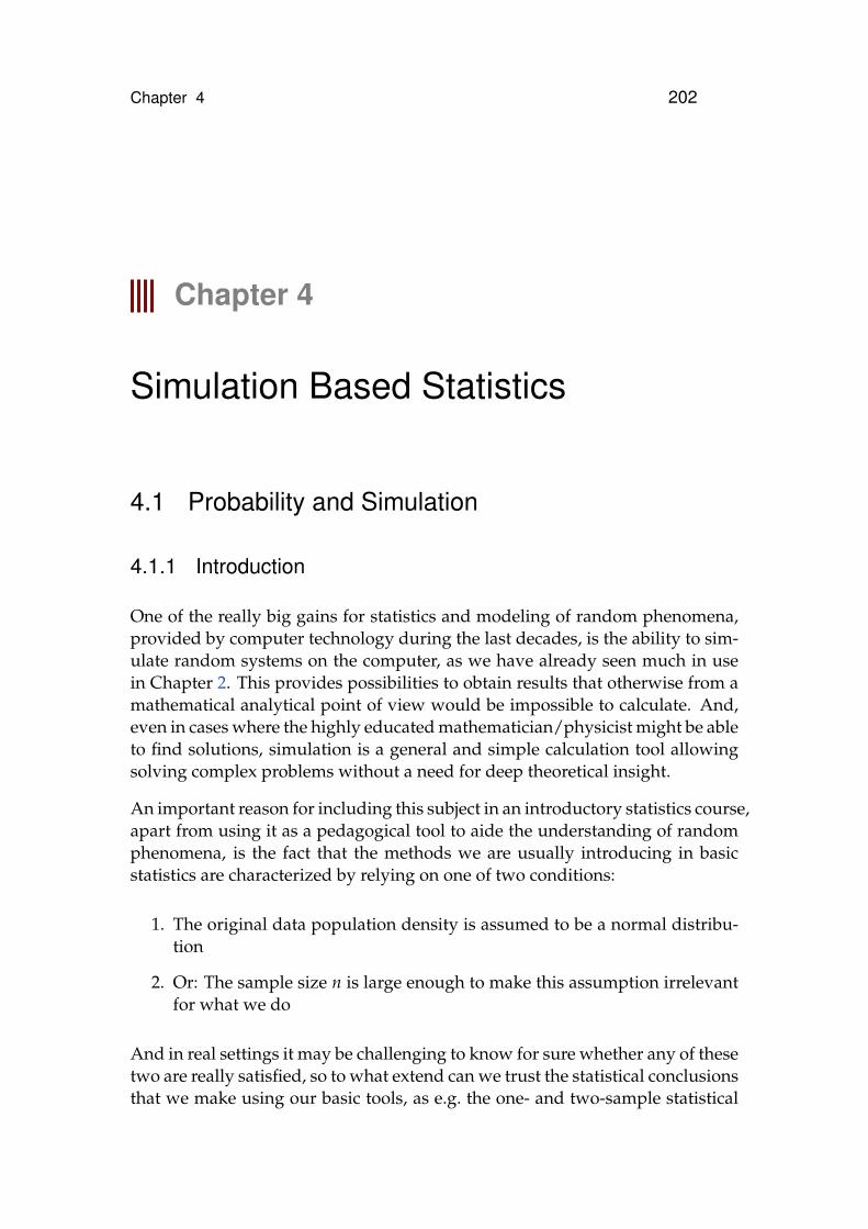
Chapter 4 202
Chapter 4
Simulation Based Statistics
4.1 Probability and Simulation
4.1.1 Introduction
One of the really big gains for statistics and modeling of random phenomena,provided by computer technology during the last decades, is the ability to sim-ulate random systems on the computer, as we have already seen much in usein Chapter 2. This provides possibilities to obtain results that otherwise from amathematical analytical point of view would be impossible to calculate. And,even in cases where the highly educated mathematician/physicist might be ableto find solutions, simulation is a general and simple calculation tool allowingsolving complex problems without a need for deep theoretical insight.
An important reason for including this subject in an introductory statistics course,apart from using it as a pedagogical tool to aide the understanding of randomphenomena, is the fact that the methods we are usually introducing in basicstatistics are characterized by relying on one of two conditions:
1. The original data population density is assumed to be a normal distribu-tion
2. Or: The sample size n is large enough to make this assumption irrelevantfor what we do
And in real settings it may be challenging to know for sure whether any of thesetwo are really satisfied, so to what extend can we trust the statistical conclusionsthat we make using our basic tools, as e.g. the one- and two-sample statistical

Chapter 4 4.1 PROBABILITY AND SIMULATION 203
methods presented in Chapter 3. And how should we do the basic statisticalanalysis if we even become convinced that none of these two conditions are ful-filled? Statistical data analysis based on simulation tools is a valuable tool tocomplete the tool box of introductory statistics. It can be used to do statisticalcomputing for other features than just means, and for other population distri-butions than the normal. It can also be used to investigate whether some of ourassumptions appear reasonable. We already saw an example of this in relationto the qq-plots in Chapter 3.1.9.
In fact, it will become clear that the simulation tools presented here will makeus rapidly able to perform statistical analysis that goes way beyond what histor-ically has been introduced in basic statistics classes or textbooks. Unfortunately,the complexity of real life engineering applications and data analysis challengescan easily go beyond the settings that we have time to cover within an intro-ductory exposition. With the general simulation tool in our tool box, we havea multitool that can be used for (and adapted to) basically almost any level ofcomplexity that we will meet in our future engineering activity.
The classical statistical practice would be to try to ensure that the data we’reanalyzing behaves like a normal distribution: symmetric and bell-shaped his-togram. In Chapter 3 we also learned that we can make a normal q-q plot toverify this assumption in practice, and possibly transform the data to get themcloser to being normal. The problem with small samples is that it even withthese diagnostic tools can be difficult to know whether the underlying distribu-tion really is ”normal” or not.
And in some cases the assumption of normality after all simply may be obvi-uosly wrong. For example, when the response scale we work with is far frombeing quantitative and continuous - it could be a scale like ”small”, ”medium”and ”large” - coded as 1, 2 and 3. We need tools that can do statistical analy-sis for us WITHOUT the assumption that the normal distribution is the rightmodel for the data we observe and work with.
Traditionally, the missing link would be covered by the so-called non-parametrictests. In short this is a collection of methods that make use of data at a morecoarse level, typically by focusing on the rank of the observations instead of theactual values of the observations. So in a paired t-test setup, for example, onewould just count how many times the observations in one sample is bigger thanin the other – instead of calculating the differences. In that way you can makestatistical tests without using the assumption of an underlying normal distribu-tion. There are a large number of such non-parametric tests for different setups.Historically, before the computer age, it was the only way to really handle suchsituations in practice. These tests are all characterized by the fact that they aregiven by relatively simple computational formulas which in earlier times easily

Chapter 4 4.1 PROBABILITY AND SIMULATION 204
could be handled. For small sample statistics with questionable distributionalsettings, these tools maintain to offer a robust set of basic statistical procedures.
The simulation based methods that we now present instead have a couple ofcrucial advantages to the traditional non-parametric methods:
• Confidence intervals are much easier to achieve
• They are much easier to apply in more complex situations
• They scale better to modern time big data analysis
4.1.2 Simulation as a general computational tool
Basically, the strength of the simulation tool is that one can compute arbitraryfunctions of random variables and their outcomes. In other words one can findprobabilities of complicated outcomes. As such, simulation is really not a statis-tical tool, but rather a probability calculus tool. However, since statistics essen-tially is about analysing and learning from real data in the light of certain proba-bilities, the simulation tool indeed becomes of statistical importance, which wewill exemplify very specifically below. Before starting with exemplifying thepower of simulation as a general computational tool, we refer to the introduc-tion to simulation in Chapter 2 – in particular read first Section 2.6, Example2.15 and thereafter Section 2.6.
Example 4.1 Rectangular plates
A company produces rectangular plates. The length of plates (in meters), X is as-sumed to follow a normal distribution N(2, 0.012) and the width of the plates (inmeters), Y are assumed to follow a normal distribution N(3, 0.022). We’re hencedealing with plates of size 2× 3 meters, but with errors in both length and width.Assume that these errors are completely independent. We are interested in the areaof the plates which of course is given by A = XY. This is a non-linear function of Xand Y, and actually it means that we, with the theoretical tools we presented so farin the material, cannot figure out what the mean area really is, and not at all whatthe standard deviation would be in the areas from plate to plate, and we would defi-nitely not know how to calculate the probabilities of various possible outcomes. Forexample, how often such plates have an area that differ by more than 0.1 m2 fromthe targeted 6 m2? One statement summarizing all our lack of knowledge at thispoint: we do not know the probability distribution of the random variable A andwe do not know how to find it! With simulation, it is straightforward: one can findall relevant information about A by just simulating the X and Y a high number of

Chapter 4 4.1 PROBABILITY AND SIMULATION 205
times, and from this compute A just as many times, and then observe what happensto the values of A. The first step is then given by:
## Number of simulationsk <- 10000## Simulate X, Y and then AX <- rnorm(k, 2, 0.01)Y <- rnorm(k, 3, 0.02)A <- X*Y
The R object A now contains 10.000 observations of A. The expected value and thestandard deviation for A are simply found by calculating the average and standarddeviation for the simulated A-values:
mean(A)
[1] 6
sd(A)
[1] 0.04957
and the desired probability, P(|A− 6| > 0.1) = 1− P(5.9 ≤ A ≤ 6.1) is found bycounting how often the incident actually occurs among the k outcomes of A:
mean(abs(A-6)>0.1)
[1] 0.0439
The code abs(A-6)>0.1 creates a vector with values TRUE or FALSE depending onwhether the absolute value of A− 6 is greater than 0.1 or not. When you add (sum)these the TRUE is automatically translated into 1 and FALSE automatically set to 0, bywhich the desired count is available, and divided by the total number of simulationsk by mean().
Note, that if you do this yourself without using the same seed value you will notget exactly the same result. It is clear that this simulation uncertainty is somethingwe must deal with in practice. The size of this will depend on the situation andon the number of simulations k. We can always get a first idea of it in a specificsituation simply by repeating the calculation a few times and note how it varies.

Chapter 4 4.1 PROBABILITY AND SIMULATION 206
Indeed, one could then formalize such an investigation and repeat the simulationmany times, to get an evaluation of the simulation uncertainty. We will not pursuethis further here. When the target of the computation is in fact a probability, as in thelatter example here, you can alternatively use standard binomial statistics, which iscovered in Chapter 2 and Chapter 7. For example, with k = 100000 the uncertainty
for a calculated proportion of around 0.044 is given by:√
0.044(1−0.044)100000 = 0.00065. Or
for example, with k = 10000000 the uncertainty is 0.000065. The result using sucha k was 0.0455 and because we’re a bit unlucky with the rounding position we canin practice say that the exact result rounded to 3 decimal places are either 0.045 or0.046. In this way, a calculation which is actually based on simulation is turned intoan exact one in the sense that rounded to 2 decimal places, the result is simply 0.05.
4.1.3 Propagation of error
Within chemistry and physics one may speak of measurement errors and howmeasurement errors propagate/accumulate if we have more measurements and/oruse these measurements in subsequent formulas/calculations. First of all: Thebasic way to ”measure an error”, that is, to quantify a measurement error is bymeans of a standard deviation. As we know, the standard deviation expressesthe average deviation from the mean. It is clear it may happen that a measur-ing instrument also on average measures wrongly (off the target). This is called”bias”, but in the basic setting here, we assume that the instrument has no bias.
Hence, reformulated, an error propagation problem is a question about howthe standard deviation of some function of the measurements depends on thestandard deviations for the individual measurement: let X1, . . . , Xn be n mea-surements with standard deviations (average measurement errors) σ1, . . . , σn.As usual in this material, we assume that these measurement errors are inde-pendent of each other. There are extensions of the formulas that can handledependencies, but we omit those here. We must then in a general formulationbe able to find
σ2f (X1,...,Xn)
= V( f (X1, . . . , Xn)). (4-1)
Chapter 4 4.1 PROBABILITY AND SIMULATION 207
Remark 4.2 For the thoughtful reader: Measurement errors, er-rors and variances
Although we motivate this entire treatment by the measurement error termi-nology, often used in chemistry and physics, actually everything is validfor any kind of errors, be it “time-to-time” production errors, or “substance-to-substance” or “tube-to-tube” errors. What the relevant kind of er-rors/variabilities are depends on the situation and may very well be mixedtogether in applications. But, the point is that as long as we have a relevanterror variance, we can work with the concepts and tools here. It does nothave to have a “pure measurement error” interpretation.
Actually, we have already in this course seen the linear error propagation rule,in Theorem in 2.56, which then can be restated here as
If f (X1, . . . , Xn) =n
∑i=1
aiXi, then σ2f (X1,...,Xn)
=n
∑i=1
a2i σ2
i .
There is a more general non-linear extension of this, albeit theoretically only anapproximate result, which involves the partial derivative of the function f withrespect to the n variables:
Method 4.3 The non-linear approximative error propagation rule
If X1, . . . , Xn are independent random variables with variances σ21 , . . . , σ2
nand f is a (potentially non-linear) function of n variables, then the varianceof the f -transformed variables can be approximated linearly by
σ2f (X1,...,Xn)
=n
∑i=1
(∂ f∂xi
)2
σ2i , (4-2)
where ∂ f∂xi
is the partial derivative of f with respect to the i’th variable
In practice one would have to insert the actual measurement values x1, . . . , xnof X1, . . . , Xn in the partial derivatives to apply the formula in practice, see theexample below. This is a pretty powerful tool for the general finding of (ap-proximate) uncertainties for complicated functions of many measurements orfor that matter: complex combinations of various statistical quantities. Whenthe formula is used for the latter, it is also in some contexts called the ”deltarule” (which is mathematically speaking a so-called first-order (linear) Taylorapproximations to the non-linear function f ). We bring it forward here, because
Chapter 4 4.1 PROBABILITY AND SIMULATION 208
as an alternative to this approximate formula one could use simulation in thefollowing way:
Method 4.4 Non-linear error propagation by simulation
Assume we have actual measurements x1, . . . , xn with known/assumed er-ror variances σ2
1 , . . . , σ2n:
1. Simulate k outcomes of all n measurements from assumed error distri-butions, e.g. N(xi, σ2
i ): X(j)i , j = 1 . . . , k.
2. Calculate the standard deviation directly as the observed standard de-viation of the k simulated values of f :
ssimf (X1,...,Xn)
=
√√√√ 1k− 1
k
∑i=1
( f j − f )2, (4-3)
where
f j = f (X(j)1 , . . . , X(j)
n ). (4-4)
Example 4.5
Let us continue the example with A = XY and X and Y defined as in the exampleabove. First of all note, that we already above used the simulation based error prop-agation method, when we found the standard deviation to be 0.04957 based on thesimulation. To exemplify the approximate error propagation rule, we must find thederivatives of the function f (x, y) = xy with respect to both x and y
∂ f∂x
= y∂ f∂y
= x.
Assume, that we now have two specific measurements of X and Y, for exampleX = 2.00 m and y = 3.00 m the error propagation law would provide the followingapproximate calculation of the ”uncertainty error variance of the area result” 2.00 m ·3.00 m = 6.00 m2, namely
σ2A = y2 · 0.012 + x2 · 0.022 = 3.002 · 0.012 + 2.002 · 0.022 = 0.0025.
So, with the error propagation law we are managing a part of the challenge withoutsimulating. Actually, we are pretty close to be able to find the correct theorticalvariance of A = XY using tools provided in this course. By the definition and the

Chapter 4 4.1 PROBABILITY AND SIMULATION 209
following fundamental relationship
V(X) = E(X− E(X))2 = E(X2)− E(X)2. (4-5)
So, one can actually deduce the variance of A theoretically, it is only necessaryto know in addition that for independent random variables: E(XY) = E(X)E(Y)(which by the way then also tells us that E(A) = E(X)E(Y) = 6)
V(XY) = E[(XY)2]− E(XY)2
= E(X2)E(Y2)− E(X)2 E(Y)2
=[V(X) + E(X)2] [V(Y) + E(Y)2]− E(X)2 E(Y)2
= V(X)V(Y) + V(X)E(Y)2 + V(Y)E(X)2
= 0.012 · 0.022 + 0.012 · 32 + 0.022 · 22
= 0.00000004 + 0.0009 + 0.0016
= 0.00250004.
Note, how the approximate error propagation rule actually corresponds to the twolatter terms in the correct variance, while the first term – the product of the twovariances is ignored. Fortunately, this term is the smallest of the three in this case. Itdoes not always have to be like that. If you want to learn how to make a theoreticalderivation of the density function for A = XY then take a course in probabilitycalculation.
Note, how we in the example actually found the ”average error”, that is, theerror standard deviation by three different approaches:
1. The simulation based approach
2. The analytical, but approximate, error propagation method
3. A theoretical derivation
The simulation approach has a number of crucial advantages:
1. It offers a simple way to compute many other quantities than just the stan-dard deviation (the theoretical derivations of such other quantities couldbe much more complicated than what was shown for the variance here)
2. It offers a simple way to use any other distribution than the normal – if webelieve such better reflect reality
3. It does not rely on any linear approximations of the true non-linear rela-tions
Chapter 4 4.2 THE PARAMETRIC BOOTSTRAP 210
4.2 The parametric bootstrap
4.2.1 Introduction
Generally, a confidence interval for an unknown parameter µ is a way to ex-press uncertainty using the sampling distribution of µ = x. Hence, we use adistribution that expresses how our calculated value would vary from sampleto sample. And the sampling distribution is a theoretical consequence of theoriginal population distribution. As indicated, we have so far no method to dothis if we only have a small sample size (n < 30), and the data cannot be as-sumed to follow a normal distribution. In principle there are two approachesfor solving this problem:
1. Find/identify/assume a different and more suitable distribution for thepopulation (”the system”)
2. Do not assume any distribution whatsoever
The simulation method called bootstrapping, which in practice is to simulatemany samples, exists in two versions that can handle either of these two chal-lenges:
1. Parametric bootstrap: simulate multiple samples from the assumed distri-bution.
2. Non-parametric bootstrap: simulate multiple samples directly from thedata.
Actually, the parametric bootstrap handles in addition the situation where datacould perhaps be normally distributed, but where the calculation of interest isquite different than the average, for example, the coefficient of variation (stan-dard deviation divided by average) or the median. This would be an exampleof a non-linear function of data – thus not having a normal distribution nor a t-distribution as a sampling distribution. So, the parametric bootstrap is basicallyjust an example of the use of simulation as a general calculation tool, as intro-duced above. Both methods are hence very general and can be used in virtuallyall contexts.
In this material we have met a few of such alternative continuous distributions,e.g. the log-normal, uniform and exponential distributions. But if we thinkabout it, we have not (yet) been taught how to do any statistics (confidenceintervals and/or hypothesis testing) within an assumption of any of these. The
Chapter 4 4.2 THE PARAMETRIC BOOTSTRAP 211
parametric bootstrap is a way to do this without relying on theoretical deriva-tions of everything. As for the theoretical variance deduction above, there areindeed methods for doing such general theoretical derivations, which wouldmake us able to do statistics based on any kind of assumed distribution. Themost welknown, and in many ways also optimal, overall approach for this iscalled maximum likelihood theory. The general theory and approach of maxi-mum likelihood is not covered in this course, however it is good to know that,in fact, all the methods we present are indeed also maximum likelihood meth-ods assuming normal distributions for the population(s).
4.2.2 One-sample confidence interval for µ
Example 4.6 Confidence interval for the exponential rate or mean
Assume that we observed the following 10 call waiting times (in seconds) in a callcenter
32.6, 1.6, 42.1, 29.2, 53.4, 79.3, 2.3, 4.7, 13.6, 2.0.
If we model the waiting times using the exponential distribution, we can estimatethe mean as
µ = x = 26.08,
and hence the rate parameter λ = 1/β in the exponential distribution as (cf. 2.48)
λ = 1/26.08 = 0.03834356.
However, what if we want a 95% confidence interval for either µ = β or λ? Wehave not been tought the methods, that is, given any formulas for finding this. Thefollowing few lines of R-code, a version of the simulation based error propagationapproach from above, will do the job for us:
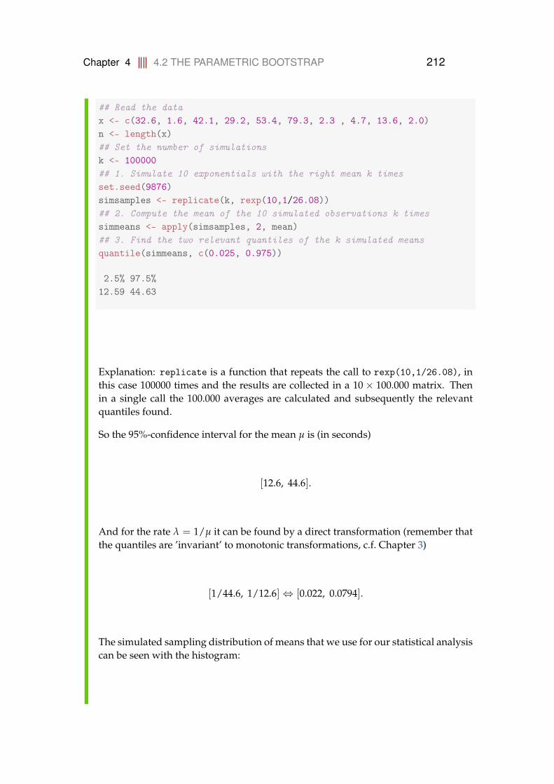
Chapter 4 4.2 THE PARAMETRIC BOOTSTRAP 212
## Read the datax <- c(32.6, 1.6, 42.1, 29.2, 53.4, 79.3, 2.3 , 4.7, 13.6, 2.0)n <- length(x)## Set the number of simulationsk <- 100000## 1. Simulate 10 exponentials with the right mean k timesset.seed(9876)simsamples <- replicate(k, rexp(10,1/26.08))## 2. Compute the mean of the 10 simulated observations k timessimmeans <- apply(simsamples, 2, mean)## 3. Find the two relevant quantiles of the k simulated meansquantile(simmeans, c(0.025, 0.975))
2.5% 97.5%12.59 44.63
Explanation: replicate is a function that repeats the call to rexp(10,1/26.08), inthis case 100000 times and the results are collected in a 10× 100.000 matrix. Thenin a single call the 100.000 averages are calculated and subsequently the relevantquantiles found.
So the 95%-confidence interval for the mean µ is (in seconds)
[12.6, 44.6].
And for the rate λ = 1/µ it can be found by a direct transformation (remember thatthe quantiles are ’invariant’ to monotonic transformations, c.f. Chapter 3)
[1/44.6, 1/12.6]⇔ [0.022, 0.0794].
The simulated sampling distribution of means that we use for our statistical analysiscan be seen with the histogram:
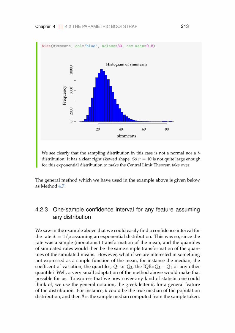
Chapter 4 4.2 THE PARAMETRIC BOOTSTRAP 213
hist(simmeans, col="blue", nclass=30, cex.main=0.8)
Histogram of simmeans
simmeans
Freq
uenc
y
20 40 60 80
020
0060
0010
000
We see clearly that the sampling distribution in this case is not a normal nor a t-distribution: it has a clear right skewed shape. So n = 10 is not quite large enoughfor this exponential distribution to make the Central Limit Theorem take over.
The general method which we have used in the example above is given belowas Method 4.7.
4.2.3 One-sample confidence interval for any feature assumingany distribution
We saw in the example above that we could easily find a confidence interval forthe rate λ = 1/µ assuming an exponential distribution. This was so, since therate was a simple (monotonic) transformation of the mean, and the quantilesof simulated rates would then be the same simple transformation of the quan-tiles of the simulated means. However, what if we are interested in somethingnot expressed as a simple function of the mean, for instance the median, thecoefficent of variation, the quartiles, Q1 or Q3, the IQR=Q3 − Q1 or any otherquantile? Well, a very small adaptation of the method above would make thatpossible for us. To express that we now cover any kind of statistic one couldthink of, we use the general notation, the greek letter θ, for a general featureof the distribution. For instance, θ could be the true median of the populationdistribution, and then θ is the sample median computed from the sample taken.
Chapter 4 4.2 THE PARAMETRIC BOOTSTRAP 214
Method 4.7 Confidence interval for any feature θ by parametricbootstrap
Assume we have actual observations x1, . . . , xn and assume that they stemfrom some probability distribution with density (pdf) f :
1. Simulate k samples of n observations from the assumed distribution fwhere the mean is set to x a
2. Calculate the statistic θ in each of the k samples θ∗1 , . . . , θ∗k
3. Find the 100(α/2)% and 100(1 − α/2)% quantiles for these,q∗100(α/2)% and q∗100(1−α/2)% as the 100(1 − α)% confidence interval:[q∗100(α/2)%, q∗100(1−α/2)%
]
a(Footnote: And otherwise chosen to match the data as good as possible: some distributionshave more than just a single mean related parameter, e.g. the normal or the log-normal. For theseone should use a distribution with a variance that matches the sample variance of the data. Evenmore generally the approach would be to match the chosen distribution to the data by the so-calledmaximum likelihood approach)
Please note again, that you can simply substitute the θ with whatever statisticsthat you are working with. This then also shows that the method box includesthe often occuring situation, where a confidence interval for the mean µ is theaim.
Example 4.8 Confidence interval for the median assuming an ex-ponential distribution
Let us look at the exponential data from the previous section and find the confidenceinterval for the median:
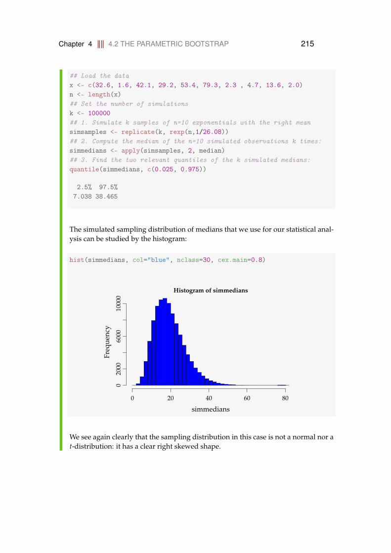
Chapter 4 4.2 THE PARAMETRIC BOOTSTRAP 215
## Load the datax <- c(32.6, 1.6, 42.1, 29.2, 53.4, 79.3, 2.3 , 4.7, 13.6, 2.0)n <- length(x)## Set the number of simulationsk <- 100000## 1. Simulate k samples of n=10 exponentials with the right meansimsamples <- replicate(k, rexp(n,1/26.08))## 2. Compute the median of the n=10 simulated observations k times:simmedians <- apply(simsamples, 2, median)## 3. Find the two relevant quantiles of the k simulated medians:quantile(simmedians, c(0.025, 0.975))
2.5% 97.5%7.038 38.465
The simulated sampling distribution of medians that we use for our statistical anal-ysis can be studied by the histogram:
hist(simmedians, col="blue", nclass=30, cex.main=0.8)
Histogram of simmedians
simmedians
Freq
uenc
y
0 20 40 60 80
020
0060
0010
000
We see again clearly that the sampling distribution in this case is not a normal nor at-distribution: it has a clear right skewed shape.

Chapter 4 4.2 THE PARAMETRIC BOOTSTRAP 216
Example 4.9 Confidence interval for Q3 assuming a normal distri-bution
Let us look at the heights data from the previous chapters and find the 99% confi-dence interval for the upper quartile: (Please note that you will find NO theory noranalytically expressed method boxes in the material to solve this challenge). Thereis one litte extra challenge for us here, since with as well the mean as the medianthere were directly applicable R-functions to do these sample computations for us,namely the R-functions mean and median. The upper quartile Q3 does not as suchhave its own R-function but it comes as part of the result of e.g. the summary functionor the quantile function. However, in one little line of R-code, we could make sucha Q3-function ourselves, e.g. by:
Q3 <- function(x){ quantile(x, 0.75) }
And now it goes exactly as before:
## load in the datax <- c(168, 161, 167, 179, 184, 166, 198, 187, 191, 179)n <- length(x)## Set the number of simulations:
k <- 100000## 1. Simulate k samples of n=10 normals with the right mean and variance:set.seed(9876)simsamples <- replicate(k, rnorm(n, mean(x), sd(x)))## 2. Compute the Q3 of the n=10 simulated observations k times:simQ3 <- apply(simsamples, 2, Q3)## 3. Find the two relevant quantiles of the k simulated medians:quantile(simQ3, c(0.005, 0.995))
0.5% 99.5%172.8 198.0
The simulated sampling distribution of upper quartiles that we use for our statisticalanalysis can be studied by the histogram:
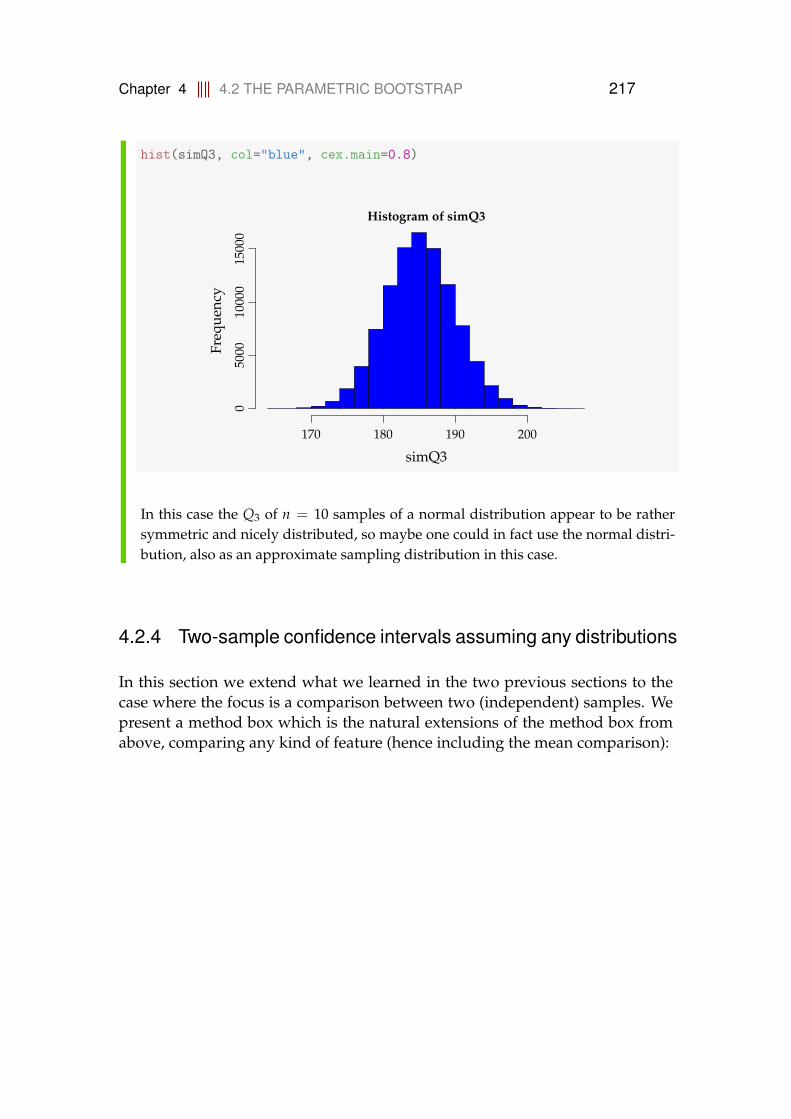
Chapter 4 4.2 THE PARAMETRIC BOOTSTRAP 217
hist(simQ3, col="blue", cex.main=0.8)
Histogram of simQ3
simQ3
Freq
uenc
y
170 180 190 200
050
0010
000
1500
0
In this case the Q3 of n = 10 samples of a normal distribution appear to be rathersymmetric and nicely distributed, so maybe one could in fact use the normal distri-bution, also as an approximate sampling distribution in this case.
4.2.4 Two-sample confidence intervals assuming any distributions
In this section we extend what we learned in the two previous sections to thecase where the focus is a comparison between two (independent) samples. Wepresent a method box which is the natural extensions of the method box fromabove, comparing any kind of feature (hence including the mean comparison):
Chapter 4 4.2 THE PARAMETRIC BOOTSTRAP 218
Method 4.10 Two-sample confidence interval for any feature com-parison θ1 − θ2 by parametric bootstrap
Assume we have actual observations x1, . . . , xn and y1, . . . , yn and assumethat they stem from some probability distributions with density f1 and f2:
1. Simulate k sets of 2 samples of n1 and n2 observations from the as-sumed distributions setting the means to µ1 = x and µ2 = y, respec-tively a
2. Calculate the difference between the features in each of the k samplesθ∗x1 − θ∗y1, . . . , θ∗xk − θ∗yk
3. Find the 100(α/2)% and 100(1 − α/2)% quantiles for these,q∗100(α/2)% and q∗100(1−α/2)% as the 100(1 − α)% confidence interval[q∗100(α/2)%, q∗100(1−α/2)%
]
a(Footnote: And otherwise chosen to match the data as good as possible: some distributionshave more than just a single mean related parameter, e.g. the normal or the log-normal. For theseone should use a distribution with a variance that matches the sample variance of the data. Evenmore generally the approach would be to match the chosen distribution to the data by the so-calledmaximum likelihood approach)
Example 4.11 CI for the difference of two means from exponentialdistributed data
Let us look at the exponential data from the previous section and compare that witha second sample of n = 12 observations from another day at the call center
9.6, 22.2, 52.5, 12.6, 33.0, 15.2, 76.6, 36.3, 110.2, 18.0, 62.4, 10.3.
Let us quantify the difference between the two days and conclude whether the callrates and/or means are any different on the two days:

Chapter 4 4.2 THE PARAMETRIC BOOTSTRAP 219
## Read the datax <- c(32.6, 1.6, 42.1, 29.2, 53.4, 79.3, 2.3 , 4.7, 13.6, 2.0)y <- c(9.6, 22.2, 52.5, 12.6, 33.0, 15.2, 76.6, 36.3, 110.2, 18.0,
62.4, 10.3)n1 <- length(x)n2 <- length(y)## Set the number of simulationsk <- 100000
## 1. Simulate k samples of each n1=10 and n2=12 exponentials## with the right meanssimXsamples <- replicate(k, rexp(n1,1/mean(x)))simYsamples <- replicate(k, rexp(n2,1/mean(y)))## 2. Compute the difference between the simulated means k timessimDifmeans <- apply(simXsamples,2,mean) - apply(simYsamples,2,mean)## 3. Find the two relevant quantiles of the k simulated differences## in sample meansquantile(simDifmeans, c(0.025, 0.975), cex.main=0.8)
2.5% 97.5%-40.74 14.12
Thus, although the mean waiting time was higher on the second day (y = 38.24 s),the range of acceptable values (the confidence interval) for the difference in meansis [−40.7, 14.1] – a pretty large range and including 0, so we have no evidence of theclaim that the two days had different mean waiting times (nor call rates then) basedon the current data.
Let us, as in previous examples take a look at the distribution of the simulated sam-ples. In a way, we do not really need this for doing the analysis, but just out ofcuriosity, and for the future it may give a idea of how far from normality the rele-vant sampling distribution really is:
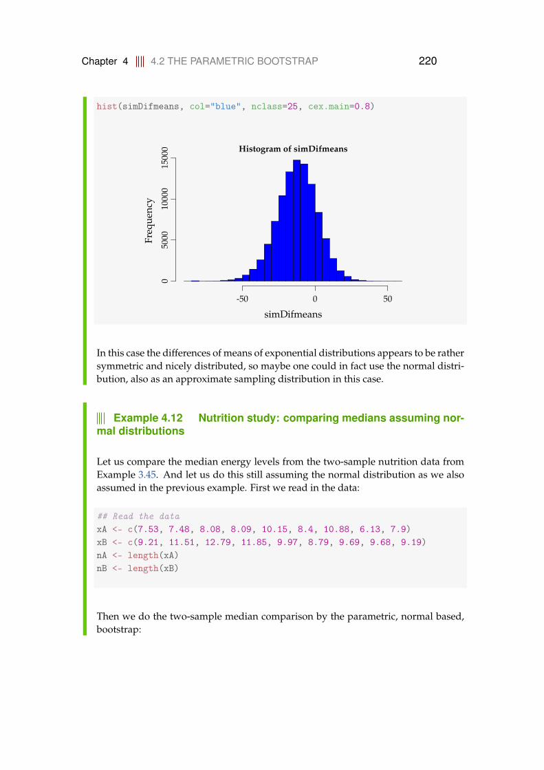
Chapter 4 4.2 THE PARAMETRIC BOOTSTRAP 220
hist(simDifmeans, col="blue", nclass=25, cex.main=0.8)
Histogram of simDifmeans
simDifmeans
Freq
uenc
y
-50 0 50
050
0010
000
1500
0
In this case the differences of means of exponential distributions appears to be rathersymmetric and nicely distributed, so maybe one could in fact use the normal distri-bution, also as an approximate sampling distribution in this case.
Example 4.12 Nutrition study: comparing medians assuming nor-mal distributions
Let us compare the median energy levels from the two-sample nutrition data fromExample 3.45. And let us do this still assuming the normal distribution as we alsoassumed in the previous example. First we read in the data:
## Read the dataxA <- c(7.53, 7.48, 8.08, 8.09, 10.15, 8.4, 10.88, 6.13, 7.9)xB <- c(9.21, 11.51, 12.79, 11.85, 9.97, 8.79, 9.69, 9.68, 9.19)nA <- length(xA)nB <- length(xB)
Then we do the two-sample median comparison by the parametric, normal based,bootstrap:
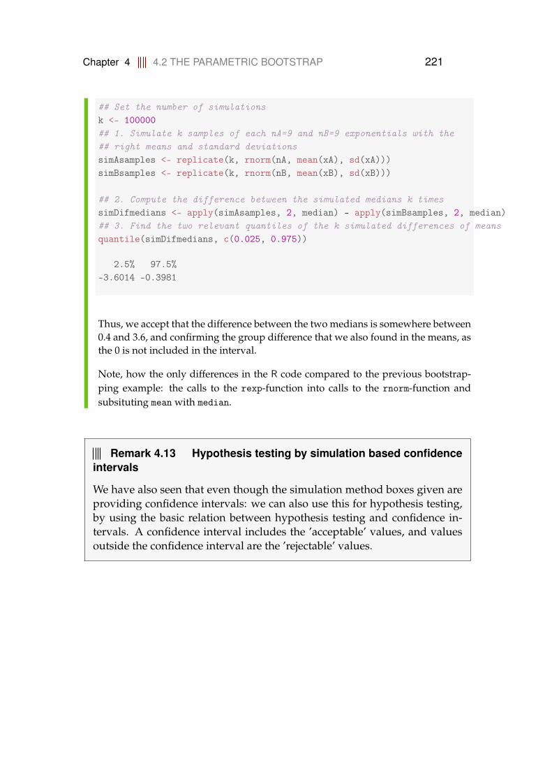
Chapter 4 4.2 THE PARAMETRIC BOOTSTRAP 221
## Set the number of simulationsk <- 100000## 1. Simulate k samples of each nA=9 and nB=9 exponentials with the## right means and standard deviationssimAsamples <- replicate(k, rnorm(nA, mean(xA), sd(xA)))simBsamples <- replicate(k, rnorm(nB, mean(xB), sd(xB)))
## 2. Compute the difference between the simulated medians k timessimDifmedians <- apply(simAsamples, 2, median) - apply(simBsamples, 2, median)## 3. Find the two relevant quantiles of the k simulated differences of meansquantile(simDifmedians, c(0.025, 0.975))
2.5% 97.5%-3.6014 -0.3981
Thus, we accept that the difference between the two medians is somewhere between0.4 and 3.6, and confirming the group difference that we also found in the means, asthe 0 is not included in the interval.
Note, how the only differences in the R code compared to the previous bootstrap-ping example: the calls to the rexp-function into calls to the rnorm-function andsubsituting mean with median.
Remark 4.13 Hypothesis testing by simulation based confidenceintervals
We have also seen that even though the simulation method boxes given areproviding confidence intervals: we can also use this for hypothesis testing,by using the basic relation between hypothesis testing and confidence in-tervals. A confidence interval includes the ’acceptable’ values, and valuesoutside the confidence interval are the ’rejectable’ values.
Chapter 4 4.3 THE NON-PARAMETRIC BOOTSTRAP 222
4.3 The non-parametric bootstrap
4.3.1 Introduction
In the introduction to the parametric bootstrap section above it was discussedthat another approach instead of finding the ’right’ distribution to use is to notassume any distribution at all. This can be done, and a way to do this simula-tion based is called the non-parametric bootstrap and is presented in this section.The section is structured as the parametric bootstrap section above – includ-ing the similar subsections and similar method boxes. So there will be twomethod boxes in this section: one for the one-sample analysis and one for thetwo-sample analysis.
In fact, the non-parametric approach could be seen as the parametric approachbut substituting the density/distribution used for the simulation by the ob-served distribution of the data, that is, the empirical cumulative distributionfunction (ecdf), cf. Chapter 1. In practice this is carried out by (re)-sampling thedata we have again and again: To get the sampling distribution of the mean (orany other feature) based on the n observations that we have in our given sam-ple, we simply again and again take new samples with n observations from theone we have. This is done ”with replacement” such that the ”new” samples,from now on called the bootstrap samples would contain some of the originalobservations in duplicates (or more) and others will not be there.
4.3.2 One-sample confidence interval for µ
We have the sample: x1, . . . , xn.
The 100(1− α)% confidence interval for µ determined by the non-parametricbootstrap is first exemplified:

Chapter 4 4.3 THE NON-PARAMETRIC BOOTSTRAP 223
Example 4.14 Women’s cigarette consumption
In a study women’s cigarette consumption before and after giving birth is explored.The following observations of the number of smoked cigarettes per day were ob-served:
before after before after8 5 13 15
24 11 15 197 0 11 12
20 15 22 06 0 15 6
20 20
This is a typical paired t-test setup, as discussed in Section 3.2.3, which then washandled by finding the 11 differences and thus transforming it into a one-samplesetup. First we read the observations into R and calculate the differences by:
## Read and calculate the differences for each woman before and afterx1 <- c(8, 24, 7, 20, 6, 20, 13, 15, 11, 22, 15)x2 <- c(5, 11, 0, 15, 0, 20, 15, 19, 12, 0, 6)dif <- x1-x2dif
[1] 3 13 7 5 6 0 -2 -4 -1 22 9
There is a random-sampling function in R (which again is based on a uniform ran-dom number generator): sample. Eg. you can get 5 repeated samples (with replace-ment - replace=TRUE) by:
t(replicate(5, sample(dif, replace=TRUE)))
[,1] [,2] [,3] [,4] [,5] [,6] [,7] [,8] [,9] [,10] [,11][1,] 13 9 -2 -4 3 -2 -1 -1 22 22 -1[2,] 3 22 6 3 22 -2 9 6 0 7 9[3,] 6 6 6 13 22 7 0 -4 0 22 7[4,] 0 9 9 3 6 9 7 9 13 -2 -1[5,] -1 22 6 -2 9 13 -1 6 22 0 9
Explanation: replicate is a function that repeats the call to sample - in this case 5times. The function t simply transposes the matrix of numbers, making it 5× 11
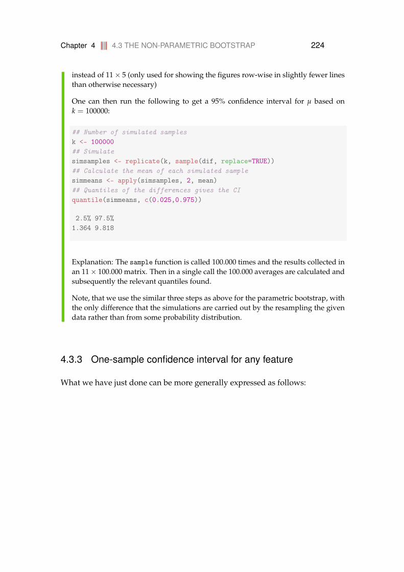
Chapter 4 4.3 THE NON-PARAMETRIC BOOTSTRAP 224
instead of 11× 5 (only used for showing the figures row-wise in slightly fewer linesthan otherwise necessary)
One can then run the following to get a 95% confidence interval for µ based onk = 100000:
## Number of simulated samplesk <- 100000## Simulatesimsamples <- replicate(k, sample(dif, replace=TRUE))## Calculate the mean of each simulated samplesimmeans <- apply(simsamples, 2, mean)## Quantiles of the differences gives the CIquantile(simmeans, c(0.025,0.975))
2.5% 97.5%1.364 9.818
Explanation: The sample function is called 100.000 times and the results collected inan 11× 100.000 matrix. Then in a single call the 100.000 averages are calculated andsubsequently the relevant quantiles found.
Note, that we use the similar three steps as above for the parametric bootstrap, withthe only difference that the simulations are carried out by the resampling the givendata rather than from some probability distribution.
4.3.3 One-sample confidence interval for any feature
What we have just done can be more generally expressed as follows:

Chapter 4 4.3 THE NON-PARAMETRIC BOOTSTRAP 225
Method 4.15 Confidence interval for any feature θ by non-parametric bootstrap
Assume we have actual observations x1, . . . , xn:
1. Simulate k samples of size n by randomly sampling among the avail-able data (with replacement)
2. Calculate the statistic θ in each of the k samples θ∗1 , . . . , θ∗k
3. Find the 100(α/2)% and 100(1 − α/2)% quantiles for these,q∗100(α/2)% and q∗100(1−α/2)% as the 100(1 − α)% confidence interval:[q∗100(α/2)%, q∗100(1−α/2)%
]
Example 4.16
Let us find the 95% confidence interval for the median cigarette consumption changein the example from above:
## The 95% CI for the median changek <- 100000simsamples <- replicate(k, sample(dif, replace = TRUE))simmedians <- apply(simsamples, 2, median)quantile(simmedians, c(0.025,0.975))
2.5% 97.5%-1 9
4.3.4 Two-sample confidence intervals
We now have two random samples: x1, . . . , xn1 and y1, . . . , yn2 . The 100(1− α)%confidence interval for θ1 − θ2 determined by the non-parametric bootstrap isdefined as:
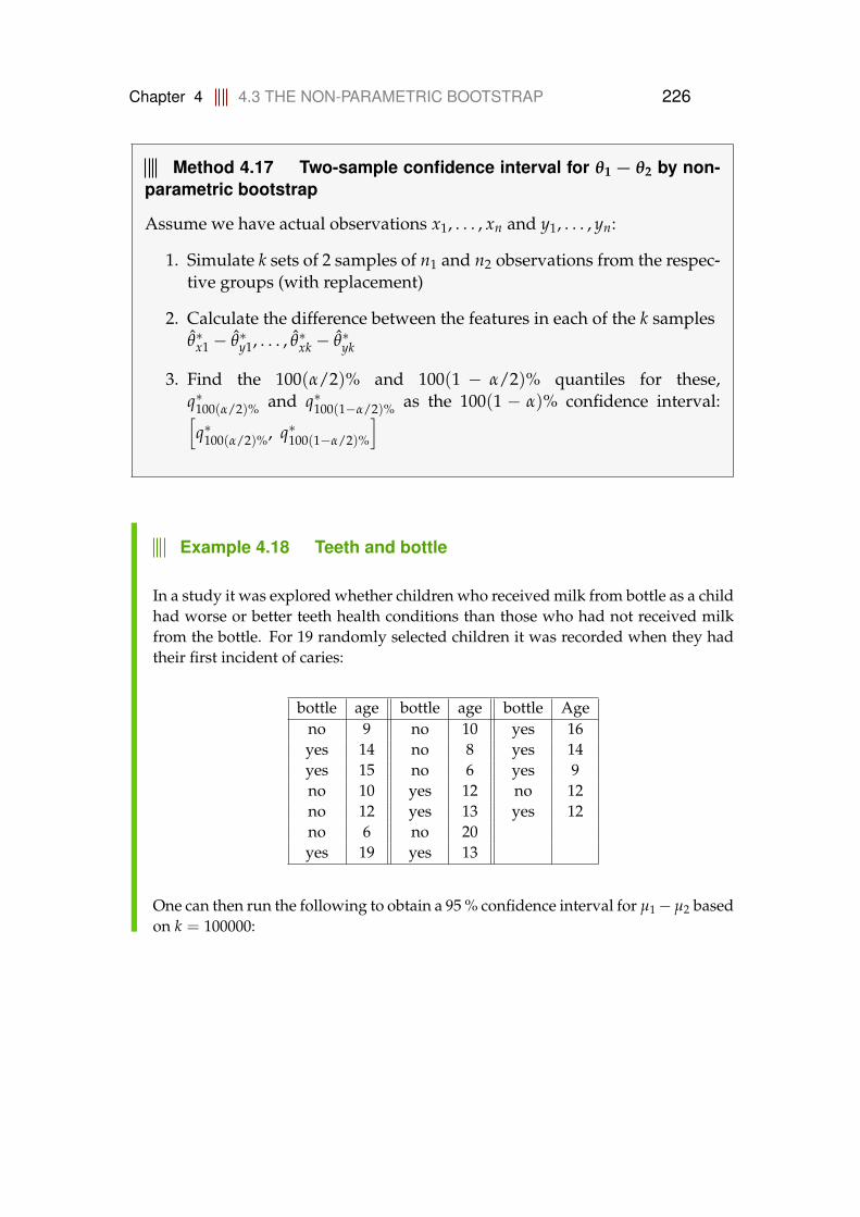
Chapter 4 4.3 THE NON-PARAMETRIC BOOTSTRAP 226
Method 4.17 Two-sample confidence interval for θ1 − θ2 by non-parametric bootstrap
Assume we have actual observations x1, . . . , xn and y1, . . . , yn:
1. Simulate k sets of 2 samples of n1 and n2 observations from the respec-tive groups (with replacement)
2. Calculate the difference between the features in each of the k samplesθ∗x1 − θ∗y1, . . . , θ∗xk − θ∗yk
3. Find the 100(α/2)% and 100(1 − α/2)% quantiles for these,q∗100(α/2)% and q∗100(1−α/2)% as the 100(1 − α)% confidence interval:[q∗100(α/2)%, q∗100(1−α/2)%
]
Example 4.18 Teeth and bottle
In a study it was explored whether children who received milk from bottle as a childhad worse or better teeth health conditions than those who had not received milkfrom the bottle. For 19 randomly selected children it was recorded when they hadtheir first incident of caries:
bottle age bottle age bottle Ageno 9 no 10 yes 16yes 14 no 8 yes 14yes 15 no 6 yes 9no 10 yes 12 no 12no 12 yes 13 yes 12no 6 no 20yes 19 yes 13
One can then run the following to obtain a 95 % confidence interval for µ1−µ2 basedon k = 100000:

Chapter 4 4.3 THE NON-PARAMETRIC BOOTSTRAP 227
## Reading in "no bottle" groupx <- c(9, 10, 12, 6, 10, 8, 6, 20, 12)## Reading in "yes bottle" groupy <- c(14,15,19,12,13,13,16,14,9,12)
## Number of simulationsk <- 100000## Simulate each sample k timessimxsamples <- replicate(k, sample(x, replace=TRUE))simysamples <- replicate(k, sample(y, replace=TRUE))## Calculate the sample mean differencessimmeandifs <- apply(simxsamples,2,mean) - apply(simysamples,2,mean)## Quantiles of the differences gives the CIquantile(simmeandifs, c(0.025,0.975))
2.5% 97.5%-6.2111 -0.1222
Example 4.19
Let us make a 99% confidence interval for the difference of medians between thetwo groups in the tooth health example:
## CI for the median differencessimmediandifs <- apply(simxsamples,2,median)-apply(simysamples,2,median)quantile(simmediandifs, c(0.005,0.995))
0.5% 99.5%-8 0

Chapter 4 4.3 THE NON-PARAMETRIC BOOTSTRAP 228
Remark 4.20 Warning: Bootstrapping may not always work wellfor small sample sizes!
The bootstrapping idea was presented here rather enthusiastically as an al-most magic method that can do everything for us in all cases. This is notthe case. Some statistics are more easily bootstrapped than others and gen-erally non-parametric bootstrap will not work well for small samples. Theinherent lack of information with small samples cannot be removed by anymagic trick. Also, there are more conceptually difficult aspects of bootstrap-ping for various purposes to improve on some of these limitations, see thenext section. Some of the "naive bootstrap" CI interval examples introducedin this chapter is likely to not have extremely good properties – the coveragepercentages might not in all cases be exactly at the aimed nominal levels.

Chapter 4 4.4 BOOTSTRAPPING – A FURTHER PERSPECTIVE 229
4.4 Bootstrapping – a further perspective
This section is not part of the syllabus, but can be seen as providing some op-tional perspectives of this very versatile method. First of all there are actuallyother principles of constructing the bootstrap confidence intervals than the onepresented here. What we have used is the so-called percentile method. Othermethods to come from the non-parametric bootstrapped samples to a confi-dence interval are called the bootstrap-t or studentized bootstrap and Bias Cor-rected Accelerated confidence intervals. These are often considered superior tothe straightforward percentile method presented above.
All of these bootstrap based confidence interval methods are also available inspecific bootstrap functions and packages in R. There are two major bootstrappackages in R: the boot and the bootstrap packages. The former is the onerecommended by the QuickR-website: (Adv. Stats, Bootstrapping) http://www.statmethods.net/advstats/bootstrapping.html.
The other package called bootstrap includes a function (also) called bootstrap.To e.g. use this one, first install this package, e.g. by:
## Install the bootstrap packageinstall.packages("bootstrap")
Example 4.21 Teeth and bottle
Now the calculation can be performed in a single call:
## Calculate the 95% CI for the Teech and bottle example abovelibrary(bootstrap)quantile(bootstrap(dif,k,mean)$thetastar, c(0.025,0.975))
2.5% 97.5%1.364 9.818
These bootstrap packages are advantageous to use when looking for confidenceintervals for more complicated functions of data.

Chapter 4 4.4 BOOTSTRAPPING – A FURTHER PERSPECTIVE 230
4.4.1 Non-parametric bootstrapping with the boot-package
Now, we will show how to use the boot-package for more general non-parametricbootstrapping than described so far. Both the bootstrap and the boot packagesrequire that the statistics that are bootstrapped in more general situations areon a specific functional form in R. The nice thing about the bootstrap pack-age is that it may handle the simple cases without this little extra complica-tion, whereas the boot package requires this for all applications, also the simpleones. However, then the boot-package has a number of other good features thatmakes it a good choice, and the point is, that for the applications coming now,the additional complexity would be needed also for the bootstrap package. Letus begin with a simple example that is already covered by our methods up tonow:
Example 4.22 Bootstrapping the mean µ by the boot-package
We will use again the women’s cigarette consumption data:
## Read and calculate the differences for each woman before and afterx1 <- c(8,24,7,20,6,20,13,15,11,22,15)x2 <- c(5,11,0,15,0,20,15,19,12,0,6)dif <- x1-x2
Our aim is to find a 95%-confidence interval for the mean difference. The additionalcomplexity mentioned is that we cannot just use the mean function as it comes, weneed to re-define it on a specific function form, where the indices enters the function:
## Define function for calculating the mean of the d indexessamplemean <- function(x, d){ mean(x[d]) }
This is a version of the mean function, where we explicitly have to specify which ofthe available observations should be used in the computation of the mean. Let uscheck the result of that:

Chapter 4 4.4 BOOTSTRAPPING – A FURTHER PERSPECTIVE 231
## Call the new functionmean(dif)
[1] 5.273
samplemean(dif,1:11)
[1] 5.273
samplemean(dif,c(1,3))
[1] 5
dif
[1] 3 13 7 5 6 0 -2 -4 -1 22 9
dif[c(1,3)]
[1] 3 7
mean(dif[c(1,3)])
[1] 5
We see that samplemean(dif,c(1,3)) means that we compute the mean of obser-vation numbers 1 and 3. Now we can use the boot package (to do what we so faralready were able to using methods from previous sections) and firstly we look atthe bootstrap distribution:
## Load the boot packagelibrary(boot)
## Non-parametric bootstrap of the mean difference:k <- 10000meandifboot <- boot(dif, samplemean, k)plot(meandifboot)
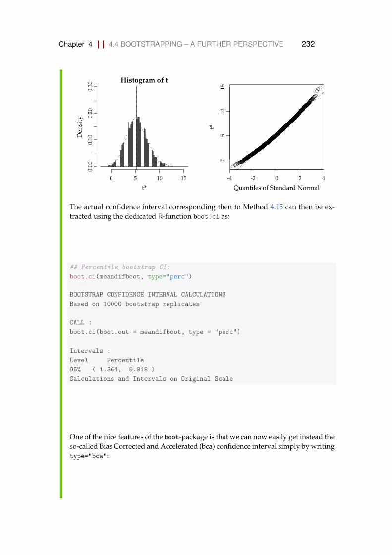
Chapter 4 4.4 BOOTSTRAPPING – A FURTHER PERSPECTIVE 232
Histogram of t
t*
Den
sity
0 5 10 15
0.00
0.10
0.20
0.30
-4 -2 0 2 4
05
1015
Quantiles of Standard Normal
t*The actual confidence interval corresponding then to Method 4.15 can then be ex-tracted using the dedicated R-function boot.ci as:
## Percentile bootstrap CI:boot.ci(meandifboot, type="perc")
BOOTSTRAP CONFIDENCE INTERVAL CALCULATIONSBased on 10000 bootstrap replicates
CALL :boot.ci(boot.out = meandifboot, type = "perc")
Intervals :Level Percentile95% ( 1.364, 9.818 )Calculations and Intervals on Original Scale
One of the nice features of the boot-package is that we can now easily get instead theso-called Bias Corrected and Accelerated (bca) confidence interval simply by writingtype="bca":

Chapter 4 4.4 BOOTSTRAPPING – A FURTHER PERSPECTIVE 233
## Bias Corrected Accelerated CI:boot.ci(meandifboot, type="bca")
BOOTSTRAP CONFIDENCE INTERVAL CALCULATIONSBased on 10000 bootstrap replicates
CALL :boot.ci(boot.out = meandifboot, type = "bca")
Intervals :Level BCa95% ( 1.636, 10.364 )Calculations and Intervals on Original Scale
And now we can apply this bca-method to any case, e.g. bootstrapping the x1 me-dian:
## Define a function for taking the median in the needed formatsamplemedian <- function(x, d) {
return(median(x[d]))}## Non-parametric bootstrap of the x1 medianb <- boot(x1,samplemedian,k)boot.ci(b, type="bca")
BOOTSTRAP CONFIDENCE INTERVAL CALCULATIONSBased on 10000 bootstrap replicates
CALL :boot.ci(boot.out = b, type = "bca")
Intervals :Level BCa95% ( 7, 20 )Calculations and Intervals on Original Scale
Or the coefficient of variation for the difference:
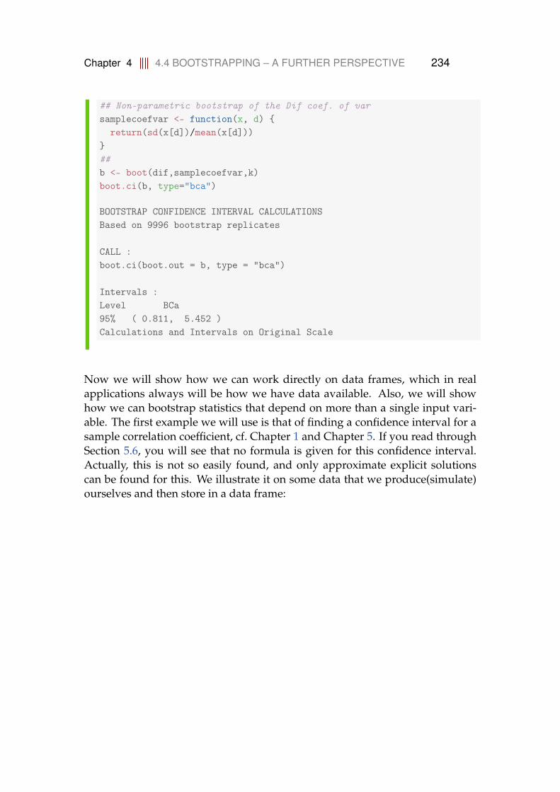
Chapter 4 4.4 BOOTSTRAPPING – A FURTHER PERSPECTIVE 234
## Non-parametric bootstrap of the Dif coef. of varsamplecoefvar <- function(x, d) {
return(sd(x[d])/mean(x[d]))}##b <- boot(dif,samplecoefvar,k)boot.ci(b, type="bca")
BOOTSTRAP CONFIDENCE INTERVAL CALCULATIONSBased on 9996 bootstrap replicates
CALL :boot.ci(boot.out = b, type = "bca")
Intervals :Level BCa95% ( 0.811, 5.452 )Calculations and Intervals on Original Scale
Now we will show how we can work directly on data frames, which in realapplications always will be how we have data available. Also, we will showhow we can bootstrap statistics that depend on more than a single input vari-able. The first example we will use is that of finding a confidence interval for asample correlation coefficient, cf. Chapter 1 and Chapter 5. If you read throughSection 5.6, you will see that no formula is given for this confidence interval.Actually, this is not so easily found, and only approximate explicit solutionscan be found for this. We illustrate it on some data that we produce(simulate)ourselves and then store in a data frame:
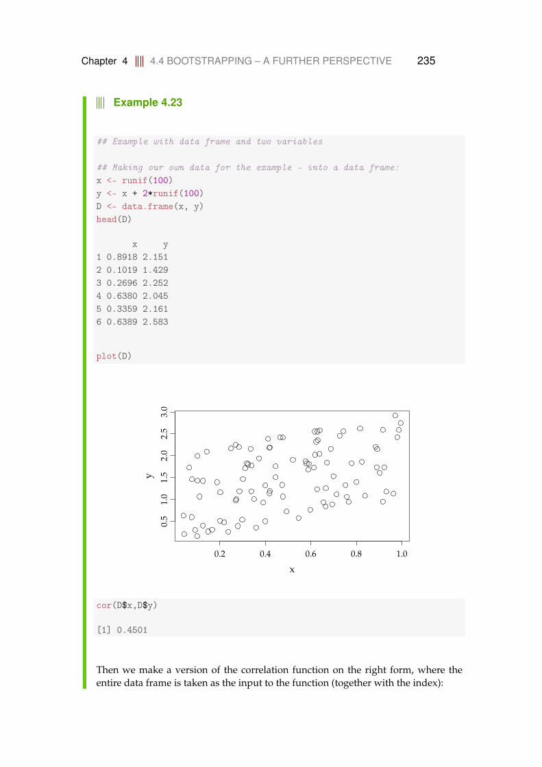
Chapter 4 4.4 BOOTSTRAPPING – A FURTHER PERSPECTIVE 235
Example 4.23
## Example with data frame and two variables
## Making our own data for the example - into a data frame:x <- runif(100)y <- x + 2*runif(100)D <- data.frame(x, y)head(D)
x y1 0.8918 2.1512 0.1019 1.4293 0.2696 2.2524 0.6380 2.0455 0.3359 2.1616 0.6389 2.583
plot(D)
0.2 0.4 0.6 0.8 1.0
0.5
1.0
1.5
2.0
2.5
3.0
x
y
cor(D$x,D$y)
[1] 0.4501
Then we make a version of the correlation function on the right form, where theentire data frame is taken as the input to the function (together with the index):

Chapter 4 4.4 BOOTSTRAPPING – A FURTHER PERSPECTIVE 236
## The correlation function on the right form:mycor <- function(D, d) {
E <- D[d,]return(cor(E$x, E$y))
}
## Check:mycor(D, 1:100)
[1] 0.4501
mycor(D, 1:15)
[1] 0.563
The E selects the chosen observations from the data frame D, and then in the compu-tations we use the variables needed from the data frame (think about how this thencan easily be extended to using any number of variables in the data frame). And wecan now do the actual bootstrap:
## Doing the bootstrap on the data frame:b <- boot(D, mycor, 10000)boot.ci(b, type="bca")
BOOTSTRAP CONFIDENCE INTERVAL CALCULATIONSBased on 10000 bootstrap replicates
CALL :boot.ci(boot.out = b, type = "bca")
Intervals :Level BCa95% ( 0.2835, 0.5964 )Calculations and Intervals on Original Scale
Our last example will show a way to bootstrap output from linear models basedon bootstrapping the entire rows of the data frame. (Other bootstrap principlesexist for linear models, e.g. bootstrapping only residuals).

Chapter 4 4.4 BOOTSTRAPPING – A FURTHER PERSPECTIVE 237
Example 4.24
We will show how to find the confidence interval for the percentage of explainedvariation in a multiple linear regression (MLR - covered in Chapter 6). We use thedata set mtcars from the boot package:
## Bootstrapping an R-Squared from an MLR using## the data set mtcars from the boot package:## (And showing how to send EXTRA stuff to your function)
# function to obtain R-Squared from the data# AND working for ANY model fit you want!!
rsq <- function(formula, data, d) {fit <- lm(formula, data=data[d,])return(summary(fit)$r.square)
}
## Bootstrapping with 1000 replicationsb <- boot(mtcars, rsq, 1000, formula=mpg~wt+disp)plot(b)
Histogram of t
t*
Den
sity
0.6 0.7 0.8 0.9
02
46
8
-3 -2 -1 0 1 2 3
0.60
0.70
0.80
0.90
Quantiles of Standard Normal
t*

Chapter 4 4.4 BOOTSTRAPPING – A FURTHER PERSPECTIVE 238
boot.ci(b, type="bca")
BOOTSTRAP CONFIDENCE INTERVAL CALCULATIONSBased on 1000 bootstrap replicates
CALL :boot.ci(boot.out = b, type = "bca")
Intervals :Level BCa95% ( 0.6308, 0.8549 )Calculations and Intervals on Original ScaleSome BCa intervals may be unstable

Chapter 4 4.5 EXERCISES 239
4.5 Exercises
Exercise 4.1 Reliability: System lifetime (simulation as a computa-tion tool)
A system consists of three components A, B and C serially connected, such thatA is positioned before B, which is again positioned before C. The system willbe functioning only so long as A, B and C are all functioning. The lifetime inmonths of the three components are assumed to follow exponential distribu-tions with means: 2 months, 3 months and 5 months, respectively (hence thereare three random variables, XA, XB and XC with exponential distributions withλA = 1/2, λB = 1/3 and λC = 1/5 resp.). A little R-help: You will probablyneed (or at least it would help) to put three variables together to make e.g. ak× 3-matrix – this can be done by the cbind function:
x <- cbind(xA,xB,xC)
And just as an example, remember from the examples in the chapter that theway to easily compute e.g. the mean of the three values for each of all the krows of this matrix is:
simmeans <- apply(x, 1, mean)
a) Generate, by simulation, a large number (at least 1000 – go for 10000 or100000 if your computer is up for it) of system lifetimes (hint: considerhow the random variable Y = System lifetime is a function of the threeX-variables: is it the sum, the mean, the median, the minimum, the maxi-mum, the range or something even different?).
b) Estimate the mean system lifetime.
c) Estimate the standard deviation of system lifetimes.
Chapter 4 4.5 EXERCISES 240
d) Estimate the probability that the system fails within 1 month.
e) Estimate the median system lifetime
f) Estimate the 10th percentile of system lifetimes
g) What seems to be the distribution of system lifetimes? (histogram etc)
Exercise 4.2 Basic bootstrap CI
(Can be handled without using R) The following measurements were given forthe cylindrical compressive strength (in MPa) for 11 prestressed concrete beams:
38.43, 38.43, 38.39, 38.83, 38.45, 38.35, 38.43, 38.31, 38.32, 38.48, 38.50.
1000 bootstrap samples (each sample hence consisting of 11 measurements)were generated from these data, and the 1000 bootstrap means were arrangedon order. Refer to the smallest as x∗(1), the second smallest as x∗(2) and so on,with the largest being x∗(1000). Assume that
x∗(25) = 38.3818,
x∗(26) = 38.3818,
x∗(50) = 38.3909,
x∗(51) = 38.3918,
x∗(950) = 38.5218,
x∗(951) = 38.5236,
x∗(975) = 38.5382,
x∗(976) = 38.5391.
Chapter 4 4.5 EXERCISES 241
a) Compute a 95% bootstrap confidence interval for the mean compressivestrength.
b) Compute a 90% bootstrap confidence interval for the mean compressivestrength.
Exercise 4.3 Various bootstrap CIs
Consider the data from the exercise above. These data are entered into R as:
x <- c(38.43, 38.43, 38.39, 38.83, 38.45, 38.35,38.43, 38.31, 38.32, 38.48, 38.50)
Now generate k = 1000 bootstrap samples and compute the 1000 means (gohigher if your computer is fine with it)
a) What are the 2.5%, and 97.5% quantiles (so what is the 95% confidenceinterval for µ without assuming any distribution)?
b) Find the 95% confidence interval for µ by the parametric bootstrap as-suming the normal distribution for the observations. Compare with theclassical analytic approach based on the t-distribution from Chapter 2.
c) Find the 95% confidence interval for µ by the parametric bootstrap as-suming the log-normal distribution for the observations. (Help: To usethe rlnorm function to simulate the log-normal distribution, we face thechallenge that we need to specify the mean and standard deviation on thelog-scale and not on the raw scale, so compute mean and standard devia-tion for log-transformed data for this R-function)
Chapter 4 4.5 EXERCISES 242
d) Find the 95% confidence interval for the lower quartile Q1 by the paramet-ric bootstrap assuming the normal distribution for the observations.
e) Find the 95% confidence interval for the lower quartile Q1 by the non-parametric bootstrap (so without any distributional assumptions)
Exercise 4.4 Two-sample TV data
A TV producer had 20 consumers evaluate the quality of two different TV flatscreens - 10 consumers for each screen. A scale from 1 (worst) up to 5 (best)were used and the following results were obtained:
TV screen 1 TV screen 21 32 41 23 42 21 32 23 41 31 2
a) Compare the two means without assuming any distribution for the twosamples (non-parametric bootstrap confidence interval and relevant hy-pothesis test interpretation).
b) Compare the two means assuming normal distributions for the two sam-ples - without using simulations (or rather: assuming/hoping that thesample sizes are large enough to make the results approximately valid).

Chapter 4 4.5 EXERCISES 243
c) Compare the two means assuming normal distributions for the two sam-ples - simulation based (parametric bootstrap confidence interval and rel-evant hypothesis test interpretation – in spite of the obviously wrong as-sumption).
Exercise 4.5 Non-linear error propagation
The pressure P, and the volume V of one mole of an ideal gas are related bythe equation PV = 8.31T, when P is measured in kilopascals, T is measured inkelvins, and V is measured in liters.
a) Assume that P is measured to be 240.48 kPa and V to be 9.987 L withknown measurement errors (given as standard deviations): 0.03 kPa and0.002 L. Estimate T and find the uncertainty in the estimate.
b) Assume that P is measured to be 240.48kPa and T to be 289.12K withknown measurement errors (given as standard deviations): 0.03kPa and0.02K. Estimate V and find the uncertainty in the estimate.
c) Assume that V is measured to be 9.987 L and T to be 289.12 K with knownmeasurement errors (given as standard deviations): 0.002 L and 0.02 K.Estimate P and find the uncertainty in the estimate.
d) Try to answer one or more of these questions by simulation (assume thatthe errors are normally distributed).

Chapter 5 244
Chapter 5
Simple Linear regression
5.1 Linear regression and least squares
In engineering applications we are often faced with the problem of determiningthe best model of some outcome given a known input
y = f (x), (5-1)
hence x is the input and the function f is the model. The task is now to findthe best model given the input variables (x) and the outcome (y). The simplestmodel, besides just a mean value (covered in Chapters 3 and 4), would be amodel where f is a linear function of x
y = β0 + β1x. (5-2)
When the outcome y is the result of some experiment, the model will not beperfect, and we need to add an error term
Yi = β0 + β1xi + εi, i = {1, . . . , n}, (5-3)
where εi is a called the error and is a (independent) random variable with ex-pectation equal zero (i.e. the mean E(εi) = 0) and some variance (V(εi) = σ2).The statistical interpretation of (5-2) is therefore that it expresses the expectedvalue of the outcome
E(Yi) = β0 + β1xi, (5-4)
also called the model prediction.
Chapter 5 5.1 LINEAR REGRESSION AND LEAST SQUARES 245
It is of course a very unusual situation that we actually know the values ofβ0 and β1 and we will have to rely on estimates based on some observations(y1, . . . , yn). As usual we express this by putting a “hat” on the parameters
yi = β0 + β1xi, (5-5)
meaning that we expect or predict yi (in mean or average) under the conditionsgiven by xi.
Note, if β1 = 0 the model is
Yi = β0 + εi, i = {1, . . . , n}, (5-6)
which is exactly the mean value model covered in Chapter 3, and the estimate ofthe mean of the population, from which the sample (i.e. (y1, . . . , yn)) was taken,is then
µ = β0. (5-7)
Example 5.1
A car manufacturer wants to find the relation between speed and fuel consumption,to do so she sets up the following model
Yi = β0 + β1xi + ε i, (5-8)
here E(Yi) is the expected fuel consumption at the speed xi. Further, there will beuncontrollable variations, e.g. due to differences in weather condition, but also non-linear effects not included in the model might be present. These variations are cap-tured by the ε i’s. We see that speed is something we control here, and we thenobserve the outcome (here fuel consumption), at different experimental conditions(speeds).
In this chapter we will deal with estimation and inference of β0, β1, and predic-tion of Yi given xi. At some point we will have realizations (or observations) ofthe outcome, in this case we write
yi = β0 + β1xi + ei, i = {1, . . . , n}. (5-9)
Now yi is a realization and ei is the deviation between the model prediction andthe actual observation: a realization of the error εi, it is called a residual. Clearly,we want the residuals to be small in some sense, the usual choice (and the onetreated in this chapter) is in the Residual Sum of Squares (RSS) sense, i.e. wewant to minimize the residual sum of squares
RSS(β0, β1) =n
∑i=1
ε2i =
n
∑i=1
(Yi − (β0 + β1xi))2, (5-10)
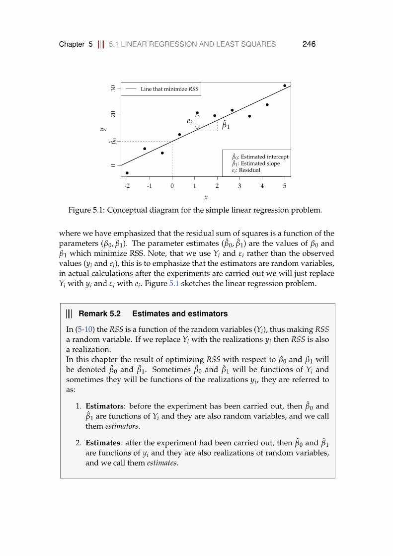
Chapter 5 5.1 LINEAR REGRESSION AND LEAST SQUARES 246
x
y
-2 -1 0 1 2 3 4 5
0β
020
30
β1ei
Line that minimize RSS
β0: Estimated interceptβ1: Estimated slopeei: Residual
Figure 5.1: Conceptual diagram for the simple linear regression problem.
where we have emphasized that the residual sum of squares is a function of theparameters (β0, β1). The parameter estimates (β0, β1) are the values of β0 andβ1 which minimize RSS. Note, that we use Yi and εi rather than the observedvalues (yi and ei), this is to emphasize that the estimators are random variables,in actual calculations after the experiments are carried out we will just replaceYi with yi and εi with ei. Figure 5.1 sketches the linear regression problem.
Remark 5.2 Estimates and estimators
In (5-10) the RSS is a function of the random variables (Yi), thus making RSSa random variable. If we replace Yi with the realizations yi then RSS is alsoa realization.In this chapter the result of optimizing RSS with respect to β0 and β1 willbe denoted β0 and β1. Sometimes β0 and β1 will be functions of Yi andsometimes they will be functions of the realizations yi, they are referred toas:
1. Estimators: before the experiment has been carried out, then β0 andβ1 are functions of Yi and they are also random variables, and we callthem estimators.
2. Estimates: after the experiment had been carried out, then β0 and β1are functions of yi and they are also realizations of random variables,and we call them estimates.

Chapter 5 5.2 PARAMETER ESTIMATES AND ESTIMATORS 247
Remark 5.3 Two types of examples
In this chapter we will use two types of examples, one is labeled “Simula-tion”, which are simulation studies intended to illustrate the consequencesof theorems and general results. While the other type of examples (not la-beled “Simulation”), are intended to illustrate the use of the theorems onpratical examples.
5.2 Parameter estimates and estimators
When β0 and β1 is a result of minimizing the function in Equation (5-10), werefer to the estimators as least squares estimators. The least squares estimators aregiven in the following theorem:
Theorem 5.4 Least squares estimators
The least squares estimators of β0 and β1 are given by
β1 =∑n
i=1(Yi − Y)(xi − x)Sxx
, (5-11)
β0 = Y− β1x, (5-12)
where Sxx = ∑ni=1(xi − x)2.
As we can see above the estimators (β1 and β2) are functions of random vari-ables (Yi and Y), and thus the estimators are themselves random variables. Wecan therefore talk about the expectation, variance and distribution of the esti-mators. In analyses with data we will of course only see realizations of Yi andwe just replace Yi and Y with their realizations yi and y. In this case we speakabout estimates of β0 and β1.
Before we go on with the proof of Theorem 5.4, the application of the theoremis illustrated in the following example:
Chapter 5 5.2 PARAMETER ESTIMATES AND ESTIMATORS 248
Example 5.5 Student height and weight
Consider the student height and weight data presented in Chapter 1,
Heights (xi) 168 161 167 179 184 166 198 187 191 179Weights (yi) 65.5 58.3 68.1 85.7 80.5 63.4 102.6 91.4 86.7 78.9
We want to find the best least squares regression line for these points, this is equiv-alent to calculating the least squares estimates of β0 and β1.
We start by finding the two sample means
x =110
(168 + 161 + . . . + 179) = 178,
y =110
(65.5 + 58.3 + . . . + 78.9) = 78.11.
The value of Sxx is calculated by
Sxx = (168− 178)2 + . . . + (179− 178)2 = 1342.
We can now calculate β1 as
β1 =1
1342((65.5− 78.11)(168− 179) + . . . + (79.9− 78.11)(179− 178)
)= 1.11,
and finally, we can calculate β0 as
β0 = 78.11− 1.11 · 178 = −120.
In R the calculation above can be done by:
## Read datax <- c(168, 161, 167, 179, 184, 166, 198, 187, 191, 179)y <- c(65.5, 58.3, 68.1, 85.7, 80.5, 63.4, 102.6, 91.4, 86.7, 78.9)
## Calculate averagesxbar <- mean(x)ybar <- mean(y)
## Parameters estimatesSxx <- sum((x - xbar)^2)beta1hat <- sum((x - xbar)*(y - ybar)) / Sxxbeta0hat <- ybar - beta1hat * xbar
Rather than using “manual” calculations in R, we can use the build in R-function lm

Chapter 5 5.2 PARAMETER ESTIMATES AND ESTIMATORS 249
D <- data.frame(x=x, y=y)fitStudents <- lm(y ~ x, data=D)summary(fitStudents)
Call:lm(formula = y ~ x, data = D)
Residuals:Min 1Q Median 3Q Max
-5.876 -1.451 -0.608 2.234 6.477
Coefficients:Estimate Std. Error t value Pr(>|t|)
(Intercept) -119.958 18.897 -6.35 0.00022 ***x 1.113 0.106 10.50 0.0000059 ***---Signif. codes: 0 '***' 0.001 '**' 0.01 '*' 0.05 '.' 0.1 ' ' 1
Residual standard error: 3.88 on 8 degrees of freedomMultiple R-squared: 0.932,Adjusted R-squared: 0.924F-statistic: 110 on 1 and 8 DF, p-value: 0.00000587
As we can see the two calculations give the same results regarding the parameterestimates. We can also see that the direct calculation in R (lm) gives some moreinformation. How to interpret and calculate these numbers will be treated in thefollowing pages.
Before we go on with the analysis of the result from lm, the proof of Theorem5.4 is presented:
Proof
Of Theorem 5.4: In order to find the minimum of the function RSS we differentiatethe residual sum of squares with respect to the parameters
∂RSS∂β0
= −2n
∑i=1
(yi − (β0 + β1xi)), (5-13)
now equating with zero we get
0 = −2n
∑i=1
(yi − (β0 + β1xi))
= −2ny + 2nβ0 + 2nβ1 x,
(5-14)
Chapter 5 5.2 PARAMETER ESTIMATES AND ESTIMATORS 250
solving for β0 gives
β0 = y− β1 x, (5-15)
and by similar calculations we get
∂RSS∂β1
=∂
∂β1
(n
∑i=1
(yi − (y− β1 x + β1xi))2
)
=∂
∂β1
(n
∑i=1
((yi − y)− β1(xi − x))2
)
= −2n
∑i=1
((yi − y)− β1(xi − x))(xi − x)
= −2
[x
∑i=1
(yi − y)(xi − x)− β1
x
∑i=1
(xi − x)2
],
(5-16)
equating with zero and solving for β1 gives
β1 =∑n
i=1(yi − y)(xi − x)∑n
i=1(xi − x)2
=∑n
i=1(yi − y)(xi − x)Sxx
.(5-17)
The estimates β0 and β1 are called least squares estimates, because they minimizethe sum of squared residuals (i.e. RSS). Replacing yi with Yi give the estimators inthe theorem.
�
When we have obtained parameter estimates in the linear regression modelabove, we would like to make quantitative statements about the uncertaintyof the parameters, and in order to design tests we will also need the probabil-ity distribution of the parameter estimators. The usual assumption is that theerrors are normal random variables
Yi = β0 + β1xi + εi, where εi ∼ N(0, σ2), (5-18)
or in other words the errors are independent identically distributed (i.i.d.) nor-mal random variables with zero mean and variance σ2. When random variablesare involved we know that repeating the experiment will result in different val-ues of the response (Yi), and therefore in different values of the parameter es-timates. To illustrate this we can make simulation experiments to analyse thebehaviour of the parameter estimates. Recall that the role of simulation exam-ples are to illustrate probabilistic behaviour of e.g. estimators, not how actualdata is analysed.

Chapter 5 5.2 PARAMETER ESTIMATES AND ESTIMATORS 251
Example 5.6 Simulation of parameter estimation
Consider the linear model
Yi = 10 + 3xi + ε i, ε i ∼ N(0, 52) (5-19)
We can make repetitions of this experiment in R
set.seed(124)n <- 10; k <- 500beta0 <- 10; beta1 <- 3; sigma <- 5x <- seq(-2, 5, length=n)y <- matrix(0, ncol=k, nrow=n)y <- y + beta0 + beta1*x + rnorm(n*k, sd=sigma)
The variable y now contains n rows and k columns, representing k experiments, foreach of the experiment we can calculate the parameter estimates:
b0 <- numeric(k); b1 <- numeric(k)for(i in 1:k){
b <- coef(lm(y[ ,i] ~ x))b0[i] <- b[1]b1[i] <- b[2]
}c(mean(b0), mean(b1))
[1] 9.955 3.008
As we can see the average of the parameter estimates (mean(b0) and mean(b1)) arevery close to the true parameter values (β0 = 10 and β1 = 3). We can of coursealso look at the empirical density (the normalized histogram, see Section 1.6.1) ofthe parameter estimates:
Empirical density of β0
b0
Den
sity
4 6 8 10 12 14 16
0.00
0.05
0.10
0.15
0.20
Empirical density of β1
b1
Den
sity
1 2 3 4 5
0.0
0.1
0.2
0.3
0.4
0.5

Chapter 5 5.2 PARAMETER ESTIMATES AND ESTIMATORS 252
The estimates seem to be rather symmetrically distributed around the true parame-ter values. It is also clear that there is some variation in the estimates: the estimatesof β0 range from about 4 to about 16 and the estimsates of β1 range from about 1 to5.
Try changing the R code (see the accompanying chapter script):
What happens to the mean value of the estimates if you change the numberof datapoints (n)?
What happens to the empirical density and the scatter plot of the parameterestimates if you change:
• The number of data points (n)?
• The range of x-values?
• The residual variance (σ2)?
• The values of β0 and β1?
In the example above we saw that the average of the parameter estimates werevery close to the true values, this is of course a nice property of an estimator.When this is the case in general, i.e. when E[βi] = βi we say that the estimatoris central. The estimators β0 and β1 are in fact central, and we show this inSection 5.2.1 below.
In order to test hypothesis about β0 and β1 we will also need to give exact state-ments about the distribution of the parameters. We saw in Example 5.6 abovethat the distributions seem to be symmetric around the true values, but we willneed more precise statements about the distributions and their variances. Thisimportant part will be dealt with in the Sections 5.3 and 5.4.
5.2.1 Estimators are central
In the linear regression model we assume that the observed values of Yi can besplit into two parts: the prediction (the part explained by the regression line(β0 + β1xi)) and the error (a random part (εi)). As usual we view our estima-tors as functions of random variables (the εi’s), so it makes sense to calculatethe expectation of the estimators. The assumption E(εi) = 0 is central for thepresented arguments, and will be used repeatedly.

Chapter 5 5.3 VARIANCE OF ESTIMATORS 253
In order to find the expectation of the parameter estimators we rewrite our esti-mators as functions of the true parameters (β0 and β1)
β1 =∑n
i=1(Yi − Y)(xi − x)Sxx
, (5-20)
inserting Yi = β0 + β1xi + εi and Y = 1n ∑n
i=1(β0 + β1xi + εi) = β0 + β1x + ε
gives
β1 =∑n
i=1 [(β0 + β1xi + εi − (β0 + β1x + ε)] (xi − x)Sxx
, (5-21)
now the sum is divided into a part which depends on εi (the random part) anda part which is independent of εi
β1 =∑n
i=1 β1(xi − x)2
Sxx+
∑ni=1(εi − ε)(xi − x)
Sxx
= β1 +∑n
i=1 εi(xi − x)Sxx
− ε ∑ni=1(xi − x)
Sxx,
(5-22)
now observe that ∑ni=1(xi − x) = 0 to get
β1 = β1 +∑n
i=1 εi(xi − x)Sxx
, (5-23)
for β0 we get
β0 = y− β1x
=1n
n
∑i=1
(β0 + β1xi + εi)−(
β1 +∑n
i=1 εi(xi − x)Sxx
)x
= β0 + β1xi +1n
n
∑i=1
εi −(
β1 +∑n
i=1 εi(xi − x)Sxx
)x
= β0 +1n
n
∑i=1
εi −(
∑ni=1 εi(xi − x)
Sxx
)x.
(5-24)
Since expectation is a linear operation (see Chapter 2) and the expectation of εiis zero we find that E[β0] = β0 and E[β1] = β1, and we say that β0, β1 are centralestimators.
5.3 Variance of estimators
In order for us to be able to construct confidence intervals for parameter esti-mates, talk about uncertainty of predictions and test hypothesis, then we will

Chapter 5 5.3 VARIANCE OF ESTIMATORS 254
need the variance of the parameter estimates as well as an estimator of the errorvariance (σ2).
Parameter variance and covariance of estimators are given in the following the-orem:
Theorem 5.7 Variance of estimators
The variance and covariance of the estimators in Theorem 5.4 are given by
V[β0] =σ2
n+
x2σ2
Sxx, (5-25)
V[β1] =σ2
Sxx, (5-26)
Cov[β0, β1] = −xσ2
Sxx, (5-27)
where σ2 is usually replaced by its estimate (σ2). The central estimator forσ2 is
σ2 =RSS(β0, β1)
n− 2. (5-28)
When the estimate of σ2 is used the variances also become estimates andwe’ll refer to them as σ2
β0and σ2
β1.
The variance of β1 is a function of the true error variance (σ2) and Sxx. For most(all reasonable) choices of the regressors (x), Sxx will be an increasing functionof n, and the variance of β1 will therefore decrease as n increases. This expressesthat we will be more certain about the estimates as we increase the number ofpoints in our sample. The same is true for the variance of β0, and the covari-ance between β1 and β0. The error variance estimate (σ) is the residual sum ofsquares divided by n− 2, the intuitive explanation for the n− 2 (rather than nor n− 1) is that if we only have two pairs (xi, yi, i.e. n = 2), it will not be possi-ble to say anything about the variation (the residuals will be zero). Or anotherphrasing is that; we have used 2 degrees of freedom to estimate β0 and β1.
Before we turn to the proof of Theorem 5.7, we will take a look at a couple ofexamples.

Chapter 5 5.3 VARIANCE OF ESTIMATORS 255
Example 5.8 (Example 5.5 cont.)
In Example 5.5 we found the parameter estimates
β0 = −119.96, β1 = 1.113,
we can now find predicted values of the dependent variable by
yi = −119.96 + 1.114 · xi,
and the values of the residuals
ei = yi − yi,
and finally the error variance estimate is
σ2 =1
10− 2
10
∑i=1
e2i .
In R we can find the results by:
beta0 <- coef(fitStudents)[1]beta1 <- coef(fitStudents)[2]e <- y - (beta0 + beta1 * x)n <- length(e)sigma <- sqrt(sum(e^2) / (n - 2))sigma.beta0 <- sqrt(sigma^2 * (1 / n + xbar^2 / Sxx))sigma.beta1 <- sqrt(sigma^2 / Sxx)c(sigma, sigma.beta0, sigma.beta1)
[1] 132.946 645.983 3.629
As usual we use standard deviations rather than variances, this also means that wecan compare with the results from lm (see Example 5.5). Again we can find ourestimates in the R-output, the parameter standard deviations are given in the secondcolumn of the coefficient matrix and the estimated standard deviation of the error iscalled residual standard error.
The simulation example (Example 5.6) can also be extended to check the equa-tions of Theorem 5.7:
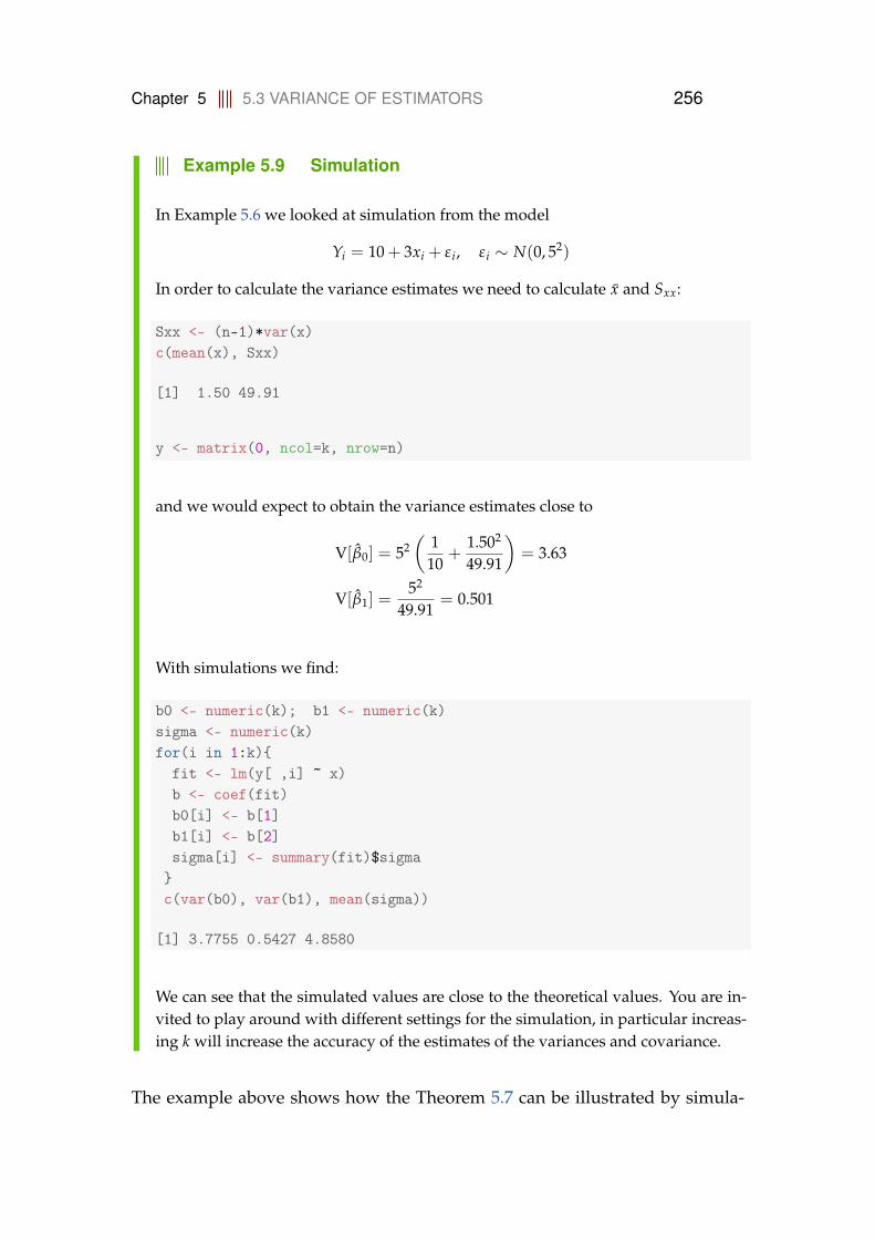
Chapter 5 5.3 VARIANCE OF ESTIMATORS 256
Example 5.9 Simulation
In Example 5.6 we looked at simulation from the model
Yi = 10 + 3xi + ε i, ε i ∼ N(0, 52)
In order to calculate the variance estimates we need to calculate x and Sxx:
Sxx <- (n-1)*var(x)c(mean(x), Sxx)
[1] 1.50 49.91
y <- matrix(0, ncol=k, nrow=n)
and we would expect to obtain the variance estimates close to
V[β0] = 52(
110
+1.502
49.91
)= 3.63
V[β1] =52
49.91= 0.501
With simulations we find:
b0 <- numeric(k); b1 <- numeric(k)sigma <- numeric(k)for(i in 1:k){
fit <- lm(y[ ,i] ~ x)b <- coef(fit)b0[i] <- b[1]b1[i] <- b[2]sigma[i] <- summary(fit)$sigma
}c(var(b0), var(b1), mean(sigma))
[1] 3.7755 0.5427 4.8580
We can see that the simulated values are close to the theoretical values. You are in-vited to play around with different settings for the simulation, in particular increas-ing k will increase the accuracy of the estimates of the variances and covariance.
The example above shows how the Theorem 5.7 can be illustrated by simula-
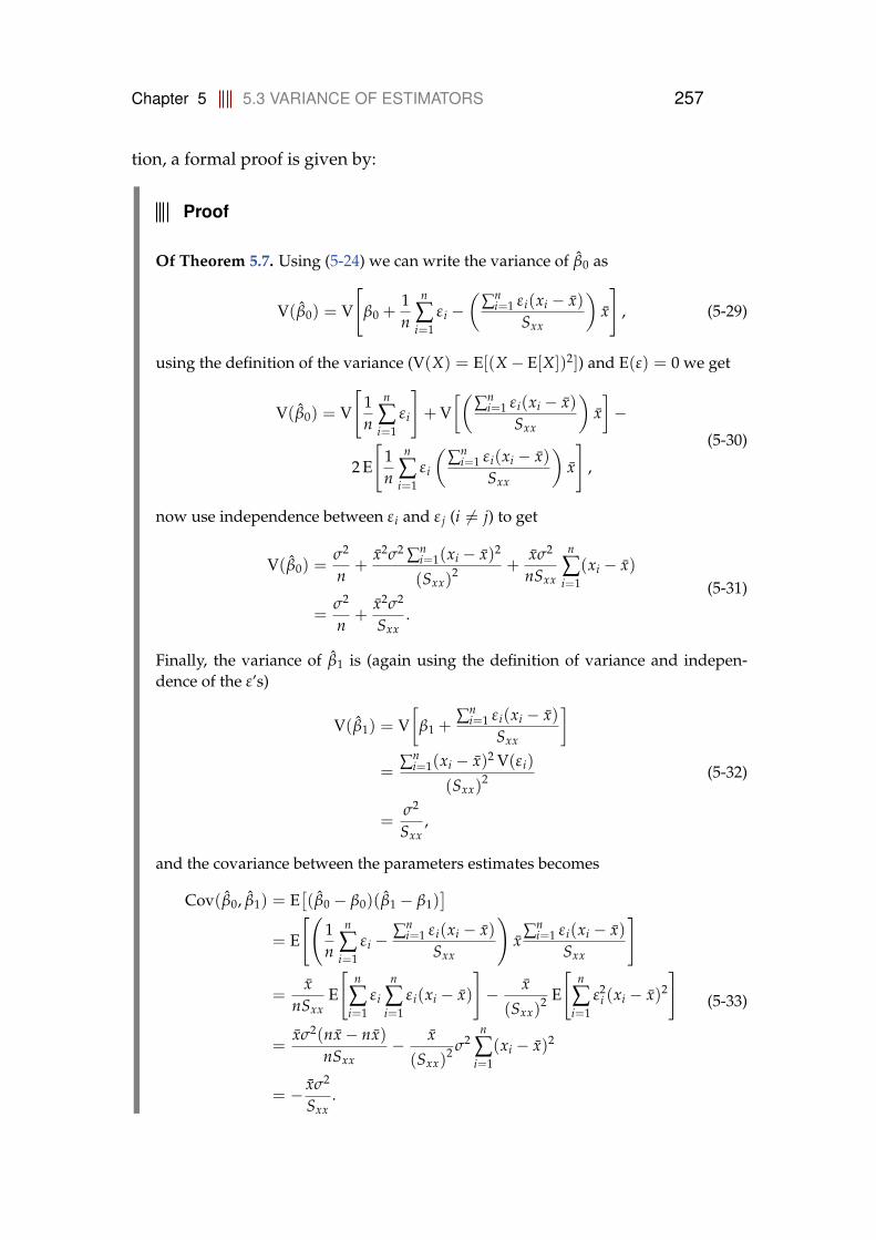
Chapter 5 5.3 VARIANCE OF ESTIMATORS 257
tion, a formal proof is given by:
Proof
Of Theorem 5.7. Using (5-24) we can write the variance of β0 as
V(β0) = V
[β0 +
1n
n
∑i=1
ε i −(
∑ni=1 ε i(xi − x)
Sxx
)x
], (5-29)
using the definition of the variance (V(X) = E[(X− E[X])2]) and E(ε) = 0 we get
V(β0) = V
[1n
n
∑i=1
ε i
]+ V
[(∑n
i=1 ε i(xi − x)Sxx
)x]−
2 E
[1n
n
∑i=1
ε i
(∑n
i=1 ε i(xi − x)Sxx
)x
],
(5-30)
now use independence between ε i and ε j (i 6= j) to get
V(β0) =σ2
n+
x2σ2 ∑ni=1(xi − x)2
(Sxx)2 +
xσ2
nSxx
n
∑i=1
(xi − x)
=σ2
n+
x2σ2
Sxx.
(5-31)
Finally, the variance of β1 is (again using the definition of variance and indepen-dence of the ε’s)
V(β1) = V[
β1 +∑n
i=1 ε i(xi − x)Sxx
]
=∑n
i=1(xi − x)2 V(ε i)
(Sxx)2
=σ2
Sxx,
(5-32)
and the covariance between the parameters estimates becomes
Cov(β0, β1) = E[(β0 − β0)(β1 − β1)
]
= E
[(1n
n
∑i=1
ε i − ∑ni=1 ε i(xi − x)
Sxx
)x ∑n
i=1 ε i(xi − x)Sxx
]
=x
nSxxE
[n
∑i=1
ε i
n
∑i=1
ε i(xi − x)
]− x
(Sxx)2 E
[n
∑i=1
ε2i (xi − x)2
]
=xσ2(nx− nx)
nSxx− x
(Sxx)2 σ2
n
∑i=1
(xi − x)2
= − xσ2
Sxx.
(5-33)
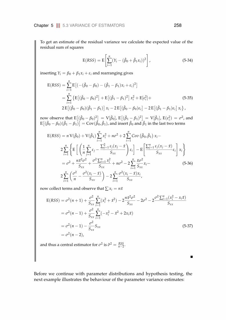
Chapter 5 5.3 VARIANCE OF ESTIMATORS 258
To get an estimate of the residual variance we calculate the expected value of theresidual sum of squares
E(RSS) = E
[n
∑i=1
(Yi − (β0 + β1xi))2
], (5-34)
inserting Yi = β0 + β1xi + ε i and rearranging gives
E(RSS) =n
∑i=1
E[(−(β0 − β0)− (β1 − β1)xi + ε i)
2]
=n
∑i=1
{E[(β0 − β0)
2]+ E[(β1 − β1)
2] x2i + E[ε2
i ]+ (5-35)
2 E[(β0 − β0)(β1 − β1)
]xi − 2 E
[(β0 − β0)ε i
]− 2 E
[(β1 − β1)ε i
]xi}
,
now observe that E[(β0 − β0)2] = V[β0], E
[(β1 − β1)
2] = V[β1], E(ε2i ) = σ2, and
E[(β0 − β0)(β1 − β1)
]= Cov(β0, β1), and insert β0 and β1 in the last two terms
E(RSS) = n V(β0) + V(β1)n
∑i=1
x2i + nσ2 + 2
n
∑i=1
Cov(
β0, β1)
xi−
2n
∑i=1
{E[(
1n
n
∑j=1
ε j −∑2
j=1 ε j(xj − xSxx
)ε i
]− E
[∑n
j=1 ε j(xj − x)Sxx
ε i
]xi
}
= σ2 +nx2σ2
Sxx+
σ2 ∑ni=1 x2
iSxx
+ nσ2 − 2n
∑i=1
xσ2
Sxxxi− (5-36)
2n
∑i=1
(σ2
n− σ2(xi − x)
Sxx
)− 2
n
∑i=1
σ2(xi − x)xi
Sxx,
now collect terms and observe that ∑ xi = nx
E(RSS) = σ2(n + 1) +σ2
Sxx
n
∑i=1
(x2i + x2)− 2
nx2σ2
Sxx− 2σ2 − 2
σ2 ∑ni=1(x2
i − xi x)Sxx
= σ2(n− 1) +σ2
Sxx
n
∑i=1
(−x2i − x2 + 2xi x)
= σ2(n− 1)− σ2
SxxSxx (5-37)
= σ2(n− 2),
and thus a central estimator for σ2 is σ2 = RSSn−2 .
�
Before we continue with parameter distributions and hypothesis testing, thenext example illustrates the behaviour of the parameter variance estimates:

Chapter 5 5.3 VARIANCE OF ESTIMATORS 259
Example 5.10 Simulation
Consider the following model
Yi = 1 + xi + ε i, ε i ∼ N(0, 1), (5-38)
also assume that xi =i−1n−1 , i = 1, . . . , n where n is the number of pairs (xi, yi). We
want to make a simulation experiment for increasing number of pairs, and extractthe parameter variance, parameter covariance and residual variance estimates. Inorder to do so we need to extract these numbers from a linear model i R. This can bedone by:
x <- seq(0, 1, length=10)y <- 1 + x + rnorm(10)## Fit the model (estimate parameter)fit <- lm(y ~ x)## Print summary of model fitsummary(fit)
Call:lm(formula = y ~ x)
Residuals:Min 1Q Median 3Q Max
-0.867 -0.596 0.232 0.374 1.295
Coefficients:Estimate Std. Error t value Pr(>|t|)
(Intercept) 0.454 0.434 1.05 0.3256x 2.521 0.731 3.45 0.0087 **---Signif. codes: 0 '***' 0.001 '**' 0.01 '*' 0.05 '.' 0.1 ' ' 1
Residual standard error: 0.738 on 8 degrees of freedomMultiple R-squared: 0.598,Adjusted R-squared: 0.548F-statistic: 11.9 on 1 and 8 DF, p-value: 0.0087
## Residual standard deviationsigma <- summary(fit)$sigma## Estimated standard deviation of parameterssummary(fit)$coefficients[ ,2]
(Intercept) x0.4336 0.7310
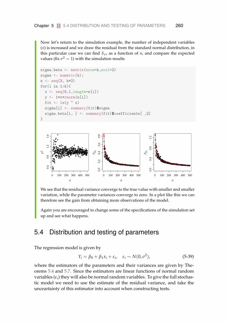
Chapter 5 5.4 DISTRIBUTION AND TESTING OF PARAMETERS 260
Now let’s return to the simulation example, the number of independent variables(x) is increased and we draw the residual from the standard normal distribution, inthis particular case we can find Sxx as a function of n, and compare the expectedvalues (fix σ2 = 1) with the simulation results
sigma.beta <- matrix(nrow=k,ncol=2)sigma <- numeric(k);n <- seq(3, k+2)for(i in 1:k){
x <- seq(0,1,length=n[i])y <- 1+x+rnorm(n[i])fit <- lm(y ~ x)sigma[i] <- summary(fit)$sigmasigma.beta[i, ] <- summary(fit)$coefficients[ ,2]
}
0 100 200 300 400 500
0.4
0.8
1.2
1.6
n
σ2
0 100 200 300 400 500
0.0
0.2
0.4
0.6
0.8
n
σβ
0
0 100 200 300 400 500
0.0
0.4
0.8
1.2
n
σβ
1
We see that the residual variance converge to the true value with smaller and smallervariation, while the parameter variances converge to zero. In a plot like this we cantherefore see the gain from obtaining more observations of the model.
Again you are encouraged to change some of the specifications of the simulation setup and see what happens.
5.4 Distribution and testing of parameters
The regression model is given by
Yi = β0 + β1xi + εi, εi ∼ N(0, σ2), (5-39)
where the estimators of the parameters and their variances are given by The-orems 5.4 and 5.7. Since the estimators are linear functions of normal randomvariables (εi) they will also be normal random variables. To give the full stochas-tic model we need to use the estimate of the residual variance, and take theunceartainty of this estimator into account when constructing tests.
Chapter 5 5.4 DISTRIBUTION AND TESTING OF PARAMETERS 261
As we already saw in Example 5.6 we cannot expect to get the true value ofthe parameter, but there will be some deviations from the true value due tothe stochastic nature of the model/real world application. The purpose of thissection is to give the precise description of the parameter distributions. We aimat testing hypothesis of the type
H0,i : βi = β0,i, (5-40)
against some alternatives. The general remarks on hypothesis testing fromChapter 3 still apply, but we will go through the specific construction for lin-ear regression here.
The central estimator of σ2 (Equation (5-28)) is χ2-distributed with n − 2 de-grees of freedom. In order to test the hypothesis in Equation (5-40) we needthe normalized distance to a null hypothesis (i.e the distance from the observedestimate β0,i to the value under the null hypothesis β0,i). From Theorem 5.7 thestandard deviations of the parameter estimates are found to
σβ0 =
√σ2
n+
x2σ2
Sxx= σ
√1n+
x2
∑ni=1(xi − x)2 , (5-41)
σβ1 =
√σ2
Sxx= σ
√1
∑ni=1(xi − x)2 , (5-42)
under the null hypothesis the normalized (with standard deviations) distancebetween the estimators and the true values are both t-distributed with n − 2degrees of freedom, and hypothesis testing and confidence intervals are basedon this t-distribution:
Theorem 5.11 Test statistics
Under the null hypothesis (β0 = β00 and β1 = β01) the statistics
Tβ0 =β0 − β0,0
σβ0
, (5-43)
Tβ1 =β1 − β0,1
σβ1
, (5-44)
are t-distributed with n − 2 degrees of freedom, and inference should bebased on this distribution.
Chapter 5 5.4 DISTRIBUTION AND TESTING OF PARAMETERS 262
Proof
The proof is omitted, but rely on the fact that β j is normally distributed, σ2β j
is χ2
distributed, and a normal random variable divided by the square root of a χ2 dis-tributed random variable is t-distributed.
�
In this material we only test two-sided hypothesis. The hypothesis can be con-cluded using p-values or critical values, in the same way as we saw for hypoth-esis regarding mean values in Chapter 3 Section 3.1.7.
Example 5.12 Example 5.8 cont.
We continue with the data from Examples 5.5 and 5.8, where we found the parame-ter estimates and the variance estimates. We want to test the hypotheses
H00 : β0 = 0 vs. H10 : β0 6= 0, (5-45)
H01 : β1 = 1 vs. H11 : β1 6= 1, (5-46)
on confidence level α = 0.05. With reference to Examples 5.5 and 5.8, and Theorem5.11, we can calculate the t-statistics as
tobs,β0 =−119.9618.897
= −6.35, (5-47)
tobs,β1 =1.113− 1
0.1059= 1.07. (5-48)
H00 is rejected if |tobs,β0 | > t1−α/2, and H01 is rejected if |tobs,β1 | > t1−α/2, as usual wecan find the critical values in R by:
qt(0.975,df=10-2)
[1] 2.306
and we see that with significance level α = 0.05, then H00 is rejected and H01 isn’t. Ifwe prefer p-values rather than critical values, these can be calculated by:
p.v0 <- 2 * (1 - pt(abs(-6.35), df=10-2))p.v1 <- 2 * (1 - pt(abs(1.07), df=10-2))c(p.v0,p.v1)
[1] 0.0002206 0.3158371

Chapter 5 5.4 DISTRIBUTION AND TESTING OF PARAMETERS 263
The p-value for the intercept (β0) is less than 0.05, while the p-value for β1 is greaterthan 0.05, hence we conclude that β0 6= 0, but we cannot reject that β1 = 1. Thesummary of linear model in R, also give t-statistics and p-values (see Example 5.5).The test statistic and the p-value for H01 is different from the one we obtained above.The reason for this is that summary() tests the default hypothesis H0i : βi = 0 againstthe alternative H1i : βi 6= 0. Even though this choice is reasonable in many situationsit does not cover all situations, and we need to calculate p-values from the summarystatistics ourselves if the hypotheses are different from the default ones.
Method 5.13 Level α t-tests for parameter
1. Formulate the null hypothesis: H0,i : βi = β0,i, and the alternative hy-pothesis H1,i : βi 6= β0,i
2. Compute the test statistic tobs,βi =βi−β0,i
σβi
3. Compute the evidence against the null hypothesis
p-valuei = 2 · P(T > |tobs,βi |) (5-49)
4. If p-valuei < α reject H0,i, otherwise accept H0,i
In many situations we will be more interested in quantifying the uncertainty ofthe parameter estimates rather than testing a specific hypothesis. This is usuallygiven in the form of confidence intervals for the parameters:
Method 5.14 Parameter confidence intervals
(1− α) confidence intervals for β0 and β1 are given by
β0 ± t1−α/2 · σβ0 , (5-50)
β1 ± t1−α/2 · σβ1 , (5-51)
where t1−α/2 is the (1− α/2)-quantile of a t-distribution with n− 2 degreesof freedom. Where σβ0 and σβ1 are calculated from the results in Theorem5.7, and Equations (5-41) and (5-42).

Chapter 5 5.4 DISTRIBUTION AND TESTING OF PARAMETERS 264
Remark 5.15
We will not show (prove) the results in Method 5.14, but see Remark 3.33.
Example 5.16 Example 5.12 cont.
Based on Method 5.14 we immediately find the 95% confidence intervals for theparameters
Iβ0 = −119.96± t0.975 · 18.897 = [−163.54,−76.38],
Iβ1 = 1.113± t0.975 · 0.1059 = [0.869, 1.357],
with the degrees of freedom for the t-distribution equal 8, and we say with highconfidence that the intervals contain the true parameter values. Of course R can findthese directly from the result returned by lm():
confint(fitStudents, level=0.95)
2.5 % 97.5 %(Intercept) -163.5348 -76.381x 0.8684 1.357
5.4.1 Confidence and prediction intervals for the line
It is clearly of interest to predict outcomes of future experiments. Here we needto distinguish between prediction intervals, where we predict the outcome ofone single experiment, and confidence intervals, where we predict the meanvalue of future outcomes. In the latter case we only need to account for theuncertainty in the parameter estimates while in the first case we will also needto account for the uncertainty of the error (the random part εi).
If we conduct a new experiment with xi = xnew the expected outcome is
ynew = β0 + β1xnew (5-52)
where the only source of variation comes from the variance of the parameterestimates, and we can calculate the variance of Ynew
V(Ynew) = V(β0 + β1xnew)
= V(β0) + V(β1xnew) + 2 Cov(β0, β1xnew),(5-53)
Chapter 5 5.4 DISTRIBUTION AND TESTING OF PARAMETERS 265
now use the calculation rules for variances and covariances (Section 2.7), andinsert the variances and the covariance from Theorem 5.7
V(Ynew) =σ2
n+
σ2x2
Sxx+
σ2x2new
Sxx− 2
σ2xxnew
Sxx
= σ2(
1n+
(xnew − x)2
Sxx
),
(5-54)
to find the variance of a single new point, we are using
Ynew = β0 + β1xnew + εnew, (5-55)
and therefore need to add the variance of the residuals (εnew is independentfrom β0 and β1)
V(Ynew) = σ2(
1 +1n+
(xnew − x)2
Sxx
). (5-56)
When we construct confidence and prediction intervals we need to account forthe fact that σ2 is estimated from data and thus use the t-distribution:
Method 5.17 Intervals for the line
The (1-α) confidence interval for the line β0 + β1xnew is
β0 + β1xnew ± t1−α/2σ
√1n+
(xnew − x)2
Sxx, (5-57)
and the (1-α) prediction interval is
β0 + β1xnew ± t1−α/2σ
√1 +
1n+
(xnew − x)2
Sxx, (5-58)
where t1−α/2 is the (1− α/2)-quantile of the t-distribution with n− 2 degreesof freedom.
Remark 5.18
We will not show the results in Method 5.17, but use Equations (5-52)-to-(5-56) and Remark 3.33.
As illustrated in Figure 5.2 the confidence interval width will approach zerofor increasing number of data points, or more precisely as n and Sxx increase

Chapter 5 5.4 DISTRIBUTION AND TESTING OF PARAMETERS 266
(but for reasonable choices of the xi’s this is equivalent). Note also that theconfidence and prediction interval widths are smallest when xnew = x. Theprediction interval width will approach 2z1−α/2 · σ as n → ∞. The differencebetween the intervals are that: while we expect (1− α) · 100% of future realiza-tions to be within the prediction interval, the confidence interval is expected tocover the true regression line. The meaning of the last statement is that if sam-ples where taken many times (i.e. the experiment repeated many times) andregression lines were fitted each time we would expect that (1− α) · 100% of theconfidence interval will cover the true regression line.
Example 5.19 Student height and weight Example (5.16 cont.)
With reference to Example 5.16 suppose we want to calculate prediction and confi-dence intervals for the line for a new student with xnew = 200 cm, the prediction isynew = 102.6 kg and the 95% confidence and prediction intervals become
Ipred = −120 + 1.113 · 200± t0.975(8) · 3.88
√1 +
110
+(178− 200)2
1342= [91.8, 113],
(5-59)
Iconf = −120 + 1.113 · 200± t0.975(8) · 3.88
√1
10+
(178− 200)2
1342= [96.5, 109],
(5-60)
where t0.975 is the 0.975-quantile of a t-distribution with n− 2 degrees of freedom.
In R the intervals can be calculated by:
predict(fitStudents, newdata=data.frame(x=200), interval="confidence",level=0.95)
fit lwr upr1 102.6 96.52 108.7
predict(fitStudents, newdata=data.frame(x=200), interval="prediction",level=0.95)
fit lwr upr1 102.6 91.77 113.4
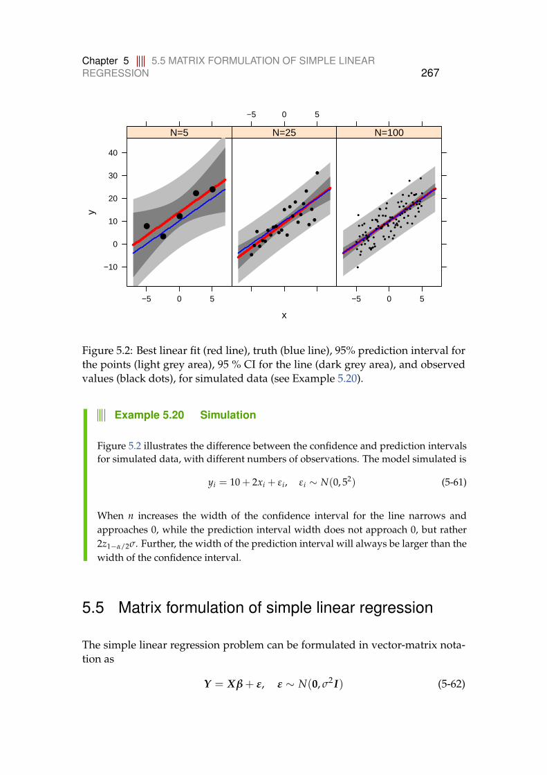
Chapter 5 5.5 MATRIX FORMULATION OF SIMPLE LINEARREGRESSION 267
x
y
−10
0
10
20
30
40
−5 0 5
●●●●●●●●●●●●●●●●●●●●●●●●●●●●●●●●●●●●●●●●●●●
●●●●●●●●
●●●●●●●●●●●
●●●●●●●●●●●●●●●●●●●
●●●●●●●●●●●●●●●●●●●●●●●●●●●●●●●●●●●●
●●●●●●●●●●●●●●●●●●●●
●●●●●●●●●●●
●●●●●●●●
●●●●●●●●●●●●●●●●●●●●●●●●●●●●●●●●●●●●●●●●●●●●
N=5
−5 0 5
●●●●●●●●●●●●●●●●●●●●●●●●●
●●●●●●●●
●●●●●●●●
●●●●●●●●
●●●●●●●●●
●●●●●●●●●●
●●●●●●●●●●
●●●●●●●●●●●●
●●●●●●●●●●
●●●●●●●●●●●●
●●●●●●●●●●●●
●●●●●●●●●●
●●●●●●●●●●
●●●●●●●●
●●●●●●●●
●●●●●●●●
●●●●●●●●
●●●●●●●●●●●●●●●●●●●●●●●●
N=25
−5 0 5
●●●●●●●●
●●●●●●●●
●●●●●●●●
●●●●●●●●
●●●●●●●●
●●●●●●●●
●●●●●●●●●●
●●●●●●●●●●
●●●●●●●●●●
●●●●●●●●●●
●●●●●●●●●●
●●
●●●●●●●●●●
●●●●●●●●●●
●●●●●●●●●●
●●●●●●●●●●
●●●●●●●●●●
●●●●●●●●
●●●●●●●●
●●●●●●●●
●●●●●●●●
●●●●●●●●
●●●●●●●●
●●
N=100
●
●
●
●●
●
●
●
●
●●
●
●
●●
●●
●
●
●
●
●
●
●
●
●
●
●
●
●
●
●
●
●
●
●
●
●
●
●
●
●
●
●
●
●
●●
●
●
●
●
●●
●
●
●
●
●
●
●
●●
●
●
●●
●●●
●
●
●
●
●
●
●
●●
●
●
●
●
●
●
●
●
●
●
●
●
●●
●
●
●
●
●
●
●
●
●
●
●
●
●
●
●
●
●
●
●
●
●
●
●
●
●●
●
●
●
●
●
●
●
●
●
●
●
Figure 5.2: Best linear fit (red line), truth (blue line), 95% prediction interval forthe points (light grey area), 95 % CI for the line (dark grey area), and observedvalues (black dots), for simulated data (see Example 5.20).
Example 5.20 Simulation
Figure 5.2 illustrates the difference between the confidence and prediction intervalsfor simulated data, with different numbers of observations. The model simulated is
yi = 10 + 2xi + ε i, ε i ∼ N(0, 52) (5-61)
When n increases the width of the confidence interval for the line narrows andapproaches 0, while the prediction interval width does not approach 0, but rather2z1−α/2σ. Further, the width of the prediction interval will always be larger than thewidth of the confidence interval.
5.5 Matrix formulation of simple linear regression
The simple linear regression problem can be formulated in vector-matrix nota-tion as
Y = Xβ + ε, ε ∼ N(0, σ2I) (5-62)
Chapter 5 5.5 MATRIX FORMULATION OF SIMPLE LINEARREGRESSION 268
or
Y1...
Yn
=
1 x1...
...1 xn
[
β0β1
]+
ε1...
εn
, εi ∼ N(0, σ2) (5-63)
One of the advantages of the matrix formulation is that the analysis generalizeto higher dimensions in a straight forward way (i.e. more xs and parameters asin the following chapter). The residual sum of squares is given by
RSS = εTε = (Y − Xβ)T(Y − Xβ), (5-64)
and the parameter estimators are given by:
Theorem 5.21
The estimators of the parameters in the simple linear regression model aregiven by
β = (XTX)−1XTY , (5-65)
and the covariance matrix of the estimates is
V[β] = σ2(XTX)−1, (5-66)
and central estimate for the error variance is
σ2 =RSS
n− 2. (5-67)
Here V[β] is a matrix with elements (V[β])11 = V[β0], (V[β])22 = V[β1], and(V[β])12 = (V[β])21 = Cov[β0, β1].
When we want to find the minimum of RSS, we again need to differentiate RSSwith respect to the parameters
∂RSS∂β
= 2XT(Y − Xβ)
= 2(XTY − XTXβ).(5-68)
Solving for β gives
β = (XTX)−1XTY , (5-69)
Chapter 5 5.5 MATRIX FORMULATION OF SIMPLE LINEARREGRESSION 269
taking the expectation of β we get
E[β] = E[(XTX)−1XTY ]
= (XTX)−1XT E[Xβ + ε]
= (XTX)−1XTXβ
= β.
(5-70)
The variance of the parameters estimates are given by
V[β] = V[(XTX)−1XTY ]
= (XTX)−1XT V[Xβ + ε]X(XTX)−T
= (XTX)−1XT(V[Xβ] + V[ε])X(XTX)−T
= (XTX)−1XTσ2IX(XTX)−T
= σ2(XTX)−1XTX(XTX)−1
= σ2(XTX)−1.
(5-71)
Again a central estimate for σ2 is
σ2 =RSS(β)
n− 2, (5-72)
and the estimate of the parameter covariance matrix is
Σβ = σ2(XTX)−1. (5-73)
Marginal tests (H0 : βi = βi,0) are constructed by observing that
βi − βi,0√(Σβ)ii
∼ t(n− 2). (5-74)
The matrix calculations in R are illustrated in the next example.
Chapter 5 5.6 CORRELATION 270
Example 5.22 Student height and weight
To illustrate how the matrix formulation works in R, the student height and weightdata is worked through below:
## DataX <- cbind(1, x)n <- length(y)## Parameter estimates and variancebeta <- solve(t(X) %*% X) %*% t(X) %*% ye <- y - X %*% betas <- sqrt(sum(e^2) / (n - 2))Vbeta <- s^2 * solve(t(X) %*% X)sbeta <- sqrt(diag(Vbeta))T.stat <- beta / sbetap.value <- 2 * (1 - pt(abs(T.stat), df = n-2))## Print the resultscoef.mat <- cbind(beta, sbeta, T.stat, p.value);colnames(coef.mat) <- c("Estimates","Std.Error","t.value","p.value")rownames(coef.mat) <- c("beta0", "beta1")coef.mat; s
Estimates Std.Error t.value p.valuebeta0 0.9821 0.08786 11.18 0.000e+00beta1 1.0708 0.15210 7.04 6.373e-12[1] 0.9857
## Prediction and confidence intervalxnew <- matrix(c(1, 200), ncol=2)ynew <- xnew %*% betaVconf <- xnew %*% Vbeta %*% t(xnew)Vpred <- Vconf + s^2sqrt(c(Vconf, Vpred))
[1] 30.34 30.36
5.6 Correlation
In the analysis above we focus on situations where we are interested in onevariable (y) as a function of another variable (x). In other situations we mightbe more interested in how x and y vary together. Examples could be ecosys-tems, where the number of predators is a function of the number of preys, but

Chapter 5 5.6 CORRELATION 271
the reverse relation is also true, further both of these numbers are affected byrandom variations and knowledge of one only gives partial knowledge of theother. Another example is individual student grade in 2 different courses, be-fore any grade has been given we will expect that a high grade in one coursewill imply a high grade in the other course, but none of them is controlled orknown in advance.
In the cases above we talk about correlation analysis and to this end we willneed the sample correlation coefficient, as defined in Section 1.4.3
ρ =1
n− 1
n
∑i=1
(xi − x
sx
)(yi − y
sy
). (5-75)
In Section 1.4.3 we notated sample correlation with r, but here we use ρ, sinceit is an estimate for the correlation ρ (see Section 2.8), and imply that there is ameaningfull interpretation of the ρ.
5.6.1 Inference on the sample correlation coefficient
In order to answer the question: are X and Y correlated? We will be interestedin constructing a test of the type
H0 : ρ = 0, H1 : ρ 6= 0. (5-76)
Consider the model
Yi = β0 + β1Xi + εi, εi ∼ N(0, σ2), (5-77)
in this case we can rewrite the sample correlation as
ρ =1
n− 1
n
∑i=1
(xi − x
sx
)(yi − y
sy
)
=Sxx
n− 11
Sxx
n
∑i=1
(xi − x
sx
)(yi − y
sy
)
=Sxx
n− 11
sxsyβ1
=sx
syβ1,
(5-78)
implying that the hypothesis (5-76) can be tested by testing the hypothesis
H0 : β1 = 0; H1 : β1 6= 0. (5-79)

Chapter 5 5.6 CORRELATION 272
since clearly the relationship in Equation (5-77) can be reversed. It should benoted that we cannot use the test to construct a confidence interval for ρ.
It should be stressed that correlation does not imply causality, it just impliesthat the variables x and y vary together. As an example consider the numberof beers sold at the university bar and the number of students attending theintroductory course in statistics. Let’s say that both numbers have increasedand therefore have a high correlation coefficient, but it does not seem reasonableto conclude that students are more interested in statistics when drinking beers.A closer look might reveal that the number of enrolled students have actuallyincreased and this can indeed explain the increase in both numbers.
5.6.2 Correlation and regression
In the linear regression models we would like to measure how much of thevariation in the outcome (Y) is explained by the input (x). A commonly usedmeasure for this is the coefficient of determination (explanation) or R2-value(see also the R summary in Example 5.5).
Definition 5.23 Coefficient of determination R2
The coefficient of determination expresses the proportion of variation in theoutcome (Y) explained by the regression line
r2 = 1− ∑i(yi − yi)2
∑i(yi − y)2 . (5-80)
In order to find this we will split the variance of y into a component due to theregression line and a component due to the residual variation
s2y =
1n− 1
n
∑i=1
(yi − y)2
=1
n− 1
n
∑i=1
(β0 + β1xi + ei −1n
n
∑i=1
(β0 + β1xi + ei))2
=1
n− 1
n
∑i=1
(β1(xi − x) + ei)2
= β21s2
x +n− 2n− 1
σ2,
(5-81)
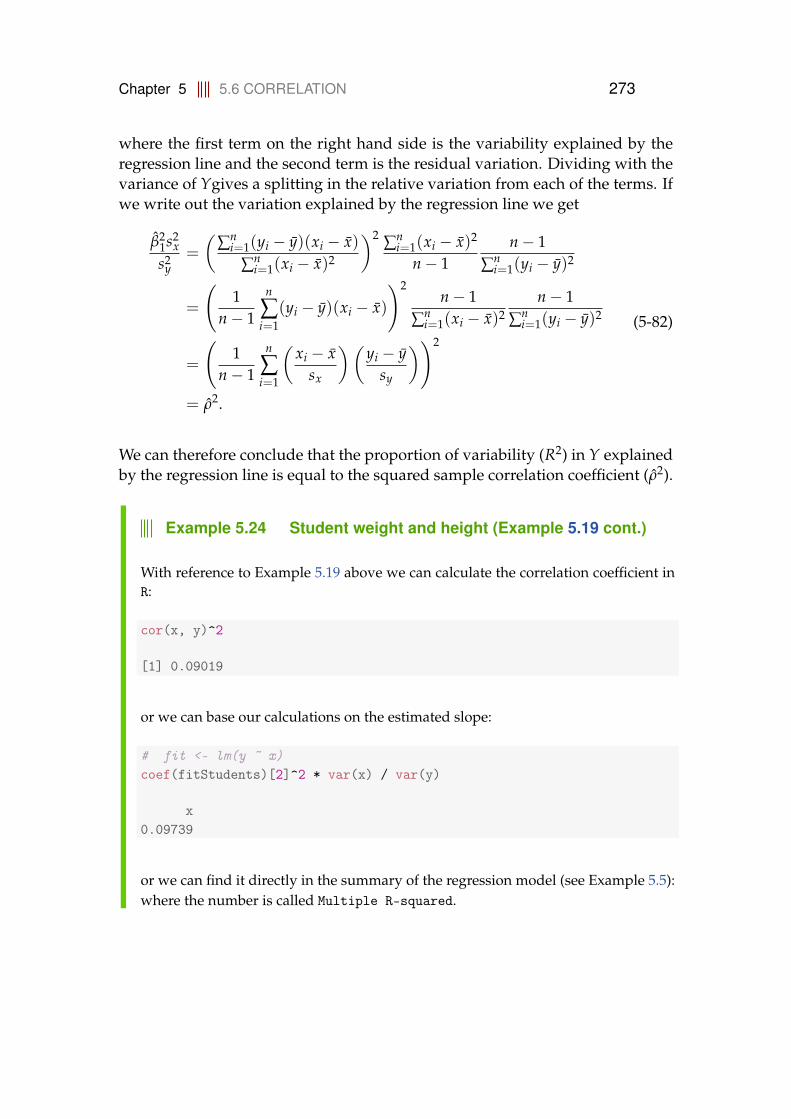
Chapter 5 5.6 CORRELATION 273
where the first term on the right hand side is the variability explained by theregression line and the second term is the residual variation. Dividing with thevariance of Ygives a splitting in the relative variation from each of the terms. Ifwe write out the variation explained by the regression line we get
β21s2
xs2
y=
(∑n
i=1(yi − y)(xi − x)∑n
i=1(xi − x)2
)2 ∑ni=1(xi − x)2
n− 1n− 1
∑ni=1(yi − y)2
=
(1
n− 1
n
∑i=1
(yi − y)(xi − x)
)2n− 1
∑ni=1(xi − x)2
n− 1∑n
i=1(yi − y)2
=
(1
n− 1
n
∑i=1
(xi − x
sx
)(yi − y
sy
))2
= ρ2.
(5-82)
We can therefore conclude that the proportion of variability (R2) in Y explainedby the regression line is equal to the squared sample correlation coefficient (ρ2).
Example 5.24 Student weight and height (Example 5.19 cont.)
With reference to Example 5.19 above we can calculate the correlation coefficient inR:
cor(x, y)^2
[1] 0.09019
or we can base our calculations on the estimated slope:
# fit <- lm(y ~ x)coef(fitStudents)[2]^2 * var(x) / var(y)
x0.09739
or we can find it directly in the summary of the regression model (see Example 5.5):where the number is called Multiple R-squared.
Chapter 5 5.7 MODEL VALIDATION 274
5.7 Model validation
So far we have discussed how to estimate parameters, predict future values,make inference etc. in the model
Yi = β0 + β1xi + εi, εi ∼ N(0, σ2). (5-83)
In all we have done so far the basic assumption is that the residuals are normallydistributed with zero mean and constant variance, and further the residuals aremutually independent. These are assumptions which should be checked andif the assumptions are not fulfilled some actions should be taken in order tofix this. This is called model validation or residual analysis and is exactly the sameidea behind the validation needed for the mean model used for t-tests in Section3.1.8, though here including a few more steps.
The normality assumption can be checked by a normal q-q plot, and the con-stant variance assumption may be checked by plotting the residuals as a func-tion of the fitted values. The normal q-q plot have been treated in Section 3.1.8and should be applied equivalently. Plotting the residuals as a function of thefitted values should not show a systematic behaviour, this means that the rangeshould be constant and the mean value should be constant, as illustrated in thefollowing example:
Example 5.25 Simulation
We consider data generated from the following three models
Y1,i = β0 + β1x1,i + ε i, ε i ∼ N(0, 1), (5-84)
Y2,i = β0 + β1x1,i + β2x2,i + ε i, ε i ∼ N(0, 1), (5-85)
Y3,i = eβ0+β1x1,i+εi , ε i ∼ N(0, 1) (5-86)
In all cases we fit the model
Yi = β0 + β1x1,i + ε i, ε i ∼ N(0, σ2), (5-87)
to the data: from the first model we would expect that the residual analysis do notshow any problems, for the second model we have a linear dependence which isnot included in the model and we should see this in the residual analysis, and thethird is a non-linear function of the residuals as well as the regressors and one wayto handle this will be discussed.
The first model is simulated, estimated and analysed by (β0 = 0, β1 = 1, and σ2 = 1):

Chapter 5 5.7 MODEL VALIDATION 275
n <-100x1 <- seq(1, 10, length=n)y <- x1 + rnorm(n)fit <- lm(y ~ x1)qqnorm(fit$residuals, pch=19, cex=0.5)qqline(fit$residuals)plot(fit$fitted.values, fit$residuals, pch=19, cex=0.5,xlab="Fitted values ($\\hat{y}_i$)", ylab="Residuals ($e_i$)")
-2 -1 0 1 2
-2-1
01
2
Normal Q-Q Plot
Theoretical Quantiles
Sam
ple
Qua
ntile
s
2 4 6 8 10
-2-1
01
2
Fitted values (yi)
Res
idua
ls(e
i)
As we can see there is no serious departure from normality and there are no patternsin the residuals as a function of the fitted values.
The second model (with β0 = 0, β1 = 1, β2 = 0.5 and σ2 = 1) is simulated, estimatedand analysed by (plot functions omitted):
x1 <- seq(1, 10, length=n)x2 <- seq(1, 10, length=n)^2y <- x1 + 0.5 * x2 + rnorm(n)fit <- lm(y ~ x1)

Chapter 5 5.7 MODEL VALIDATION 276
-2 -1 0 1 2
-4-2
02
46
8Normal Q-Q Plot
Theoretical Quantiles
Sam
ple
Qua
ntile
s
0 10 20 30 40 50
-4-2
02
46
8
Fitted values (yi)
Res
idua
ls(e
i)We see some departure from normality, but also that the residuals are related to thefitted values with a clear pattern. In the next chapter we will learn that we shouldfind the hidden dependence (x2) and include it in the model.
The third model (with β0 = 0, β1 = 1, β2 = 0.5 and σ2 = 1) is simulated, estimatedand analysed by (plot function omitted):
x1 <- seq(4, 10, length=100)y <- exp( 0.2 * x1 + rnorm(length(x1), sd = 0.15))fit <- lm(y ~ x1)
-2 -1 0 1 2
-10
12
3
Normal Q-Q Plot
Theoretical Quantiles
Sam
ple
Qua
ntile
s
2 3 4 5 6
-10
12
3
Fitted values (yi)
Res
idua
ls(e
i)
We see quite some departure from normality, and also that the variance increases asa function of the fitted values. When the variance is clearly related with the fittedvalues one should try to transform the dependent variable. The following R do theanalysis based in log-transformed data:
y <- log(y)fit <- lm(y ~ x1)
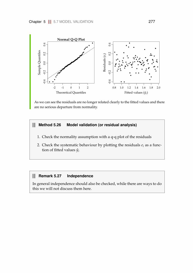
Chapter 5 5.7 MODEL VALIDATION 277
-2 -1 0 1 2
-0.4
-0.2
0.0
0.2
0.4
Normal Q-Q Plot
Theoretical Quantiles
Sam
ple
Qua
ntile
s
0.8 1.0 1.2 1.4 1.6 1.8 2.0
-0.4
-0.2
0.0
0.2
0.4
Fitted values (yi)
Res
idua
ls(e
i)As we can see the residuals are no longer related clearly to the fitted values and thereare no serious departure from normality.
Method 5.26 Model validation (or residual analysis)
1. Check the normality assumption with a q-q plot of the residuals
2. Check the systematic behaviour by plotting the residuals ei as a func-tion of fitted values yi
Remark 5.27 Independence
In general independence should also be checked, while there are ways to dothis we will not discuss them here.
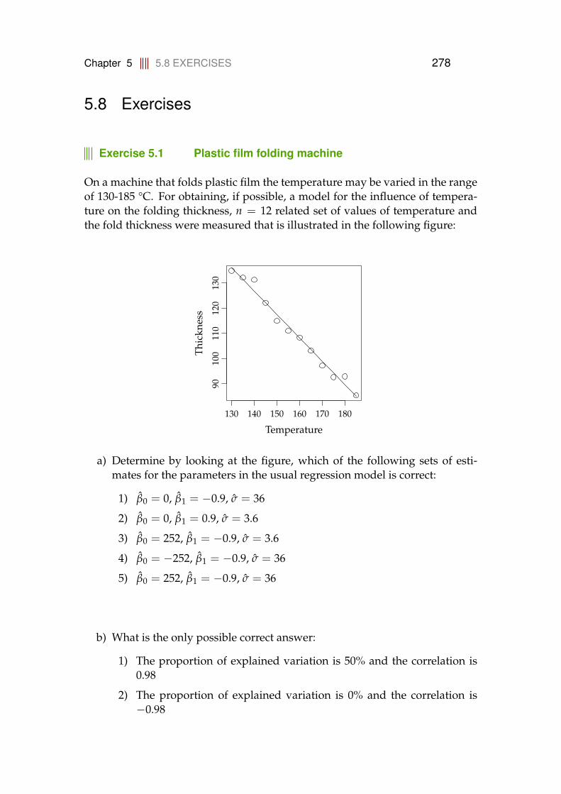
Chapter 5 5.8 EXERCISES 278
5.8 Exercises
Exercise 5.1 Plastic film folding machine
On a machine that folds plastic film the temperature may be varied in the rangeof 130-185 °C. For obtaining, if possible, a model for the influence of tempera-ture on the folding thickness, n = 12 related set of values of temperature andthe fold thickness were measured that is illustrated in the following figure:
130 140 150 160 170 180
9010
011
012
013
0
Temperature
Thic
knes
s
a) Determine by looking at the figure, which of the following sets of esti-mates for the parameters in the usual regression model is correct:
1) β0 = 0, β1 = −0.9, σ = 36
2) β0 = 0, β1 = 0.9, σ = 3.6
3) β0 = 252, β1 = −0.9, σ = 3.6
4) β0 = −252, β1 = −0.9, σ = 36
5) β0 = 252, β1 = −0.9, σ = 36
b) What is the only possible correct answer:
1) The proportion of explained variation is 50% and the correlation is0.98
2) The proportion of explained variation is 0% and the correlation is−0.98
Chapter 5 5.8 EXERCISES 279
3) The proportion of explained variation is 96% and the correlation is−1
4) The proportion of explained variation is 96% and the correlation is0.98
5) The proportion of explained variation is 96% and the correlation is−0.98
Exercise 5.2 Linear regression life time model
A company manufactures an electronic device to be used in a very wide tem-perature range. The company knows that increased temperature shortens thelife time of the device, and a study is therefore performed in which the life timeis determined as a function of temperature. The following data is found:
Temperature in Celcius (t) 10 20 30 40 50 60 70 80 90Life time in hours (y) 420 365 285 220 176 117 69 34 5
a) Calculate the 95% confidence interval for the slope in the usual linear re-gression model, which expresses the life time as a linear function of thetemperature.
b) Can a relation between temperature and life time be documented on level5%?
Exercise 5.3 Yield of chemical process
The yield y of a chemical process is a random variable whose value is consideredto be a linear function of the temperature x. The following data of correspond-ing values of x and y is found:
Temperature in °C (x) 0 25 50 75 100Yield in grams (y) 14 38 54 76 95

Chapter 5 5.8 EXERCISES 280
The average and standard deviation of temperature and yield are
x = 50, sx = 39.52847, y = 55.4, sy = 31.66702,
In the exercise the usual linear regression model is used
Yi = β0 + β1xi + εi, εi ∼ N(0, σ2ε ), i = 1, . . . , 5
a) Can a significant relationship between yield and temperature be docu-mented on the usual significance level α = 0.05?
b) Give the 95% confidence interval of the expected yield at a temperature ofxnew = 80 °C.
c) What is the upper quartile of the residuals?
Exercise 5.4 Plastic material
In the manufacturing of a plastic material, it is believed that the cooling time hasan influence on the impact strength. Therefore a study is carried out in whichplastic material impact strength is determined for 4 different cooling times. Theresults of this experiment are shown in the following table:
Cooling times in seconds (x) 15 25 35 40Impact strength in kJ/m2 (y) 42.1 36.0 31.8 28.7
The following statistics may be used:
x = 28.75, y = 34.65, Sxx = 368.75.
a) What is the 95% confidence interval for the slope of the regression model,expressing the impact strength as a linear function of the cooling time?

Chapter 5 5.8 EXERCISES 281
b) Can you conclude that there is a relation between the impact strength andthe cooling time at significance level α = 5%?
c) For a similar plastic material the tabulated value for the linear relationbetween temperature and impact strength (i.e the slope) is −0.30. If thefollowing hypothesis is tested (at level α = 0.05)
H0 : β1 = −0.30H1 : β1 6= −0.30
with the usual t-test statistic for such a test, what is the range (for t) withinwhich the hypothesis is accepted?
Exercise 5.5 Water polution
In a study of pollution in a water stream, the concentration of pollution is mea-sured at 5 different locations. The locations are at different distances to thepollution source. In the table below, these distances and the average pollutionare given:
Distance to the pollution source (in km) 2 4 6 8 10Average concentration 11.5 10.2 10.3 9.68 9.32
a) What are the parameter estimates for the three unknown parameters inthe usual linear regression model: 1) The intercept (β0), 2) the slope (β1)and 3) error standard deviation (σ)?
b) How large a part of the variation in concentration can be explained by thedistance?
c) What is a 95%-confidence interval for the expected pollution concentra-tion 7 km from the pollution source?

Chapter 5 5.8 EXERCISES 282
Exercise 5.6 Membrane pressure drop
When purifying drinking water you can use a so-called membrane filtration.In an experiment one wishes to examine the relationship between the pressuredrop across a membrane and the flux (flow per area) through the membrane.We observe the following 10 related values of pressure (x) and flux (y):
1 2 3 4 5 6 7 8 9 10Pressure (x) 1.02 2.08 2.89 4.01 5.32 5.83 7.26 7.96 9.11 9.99Flux (y) 1.15 0.85 1.56 1.72 4.32 5.07 5.00 5.31 6.17 7.04
Copy this into R to avoid typing in the data:
D <- data.frame(pressure=c(1.02,2.08,2.89,4.01,5.32,5.83,7.26,7.96,9.11,9.99),flux=c(1.15,0.85,1.56,1.72,4.32,5.07,5.00,5.31,6.17,7.04)
)
a) What is the empirical correlation between pressure and flux estimated to?Give also an interpretation of the correlation.
b) What is a 90% confidence interval for the slope β1 in the usual regressionmodel?
c) How large a part of the flux-variation (∑10i=1(yi − y)2) is not explained by
pressure differences?
d) Can you at significance level α = 0.05 reject the hypothesis that the linepasses through (0, 0)?

Chapter 5 5.8 EXERCISES 283
e) A confidence interval for the line at three different pressure levels: xAnew =
3.5, xBnew = 5.0 and xC
new = 9.5 will look as follows:
β0 + β1 · xUnew ± CU
where U then is either A, B or C. Write the constants CU in increasingorder.
Exercise 5.7 Membrane pressure drop (matrix form)
This exercise uses the data presented in Exercise 6 above.
a) Find parameters values, standard errors, t-test statistics, and p-values forthe standard hypotheses tests.
Copy this into R to avoid typing in the data:
D <- data.frame(pressure=c(1.02,2.08,2.89,4.01,5.32,5.83,7.26,7.96,9.11,9.99),flux=c(1.15,0.85,1.56,1.72,4.32,5.07,5.00,5.31,6.17,7.04)
)
b) Reproduce the above numbers by matrix vector calculations. You willneed some matrix notation in R:
– Matrix multiplication (XY): X%*%Y
– Matrix transpose (XT): t(X)
– Matrix inverse (X−1): solve(X)
– Make a matrix from vectors (X = [xT1 ; x2
2]): cbind(x1,x2)
See also Example 5.22.

Chapter 5 5.8 EXERCISES 284
Exercise 5.8 Independence and correlation
Consider the layout of independent variable in Example 5.10,
a) Show that Sxx = n·(n+1)12·(n−1) .
Hint: you can use the following relations
n
∑i=1
i =n(n + 1)
2,
n
∑i=1
i2 =n(n + 1)(2n + 1)
6.
b) Show that the asymptotic correlation between β0 and β1 is
limn→∞
ρn(β0, β1) = −√
32
.
Consider a layout of the independent variable where n = 2k and xi = 0 for i ≤ kand xi = 1 for k < i ≤ n.
c) Find Sxx for the new layout of x.
d) Compare Sxx for the two layouts of x.
e) What is the consequence for the parameter variance in the two layouts?
f) Discuss pro’s and cons for the two layouts.
Chapter 6 285
Chapter 6
Multiple Linear Regression
In Chapter 5 we described the linear regression model, when the outcome (Y) isa linear function of one regressor (x). It is natural to extend this model to includemore than one regressor, in general we can write
Yi = β0 + β1x1,i + · · ·+ βpxp,i + εi, εi ∼ N(0, σ2), (6-1)
where as usual we assume that the residuals (εi) are independent and identi-cally distributed (i.i.d.) normal random variables with zero mean and someunknown variance (σ). Note, that this is the assumption for all random vari-able error terms in models presented in this chapter, however it is not noted forevery model.
The model in Equation (6-1) is referred to as the General Linear Model (GLM),and is closely related to the ANOVA covered in a later chapter. As we will seein Section 6.2, we can also use the approach to approximate non-linear functionsof the regressors, i.e.
Yi = f (xi) + εi, εi ∼ N(0, σ2). (6-2)
The optimal set of parameters for the multiple linear regression model is foundby minimising the residual sum of squares
RSS(β0, . . . , βp) =n
∑i=1
[Yi − (β0 + β1x1,i + · · ·+ βpxp,i)
]2 , (6-3)
where n is the number of observations. The general problem is illustrated inFigure 6.1, where the black dots represent the observations (yi), the blue and redlines represent errors (ei) (the ones we minimize), and the surface representedby the grey lines is the optimal estimate (with p = 2)
yi = β0 + β1x1,i + β2x2,i, (6-4)
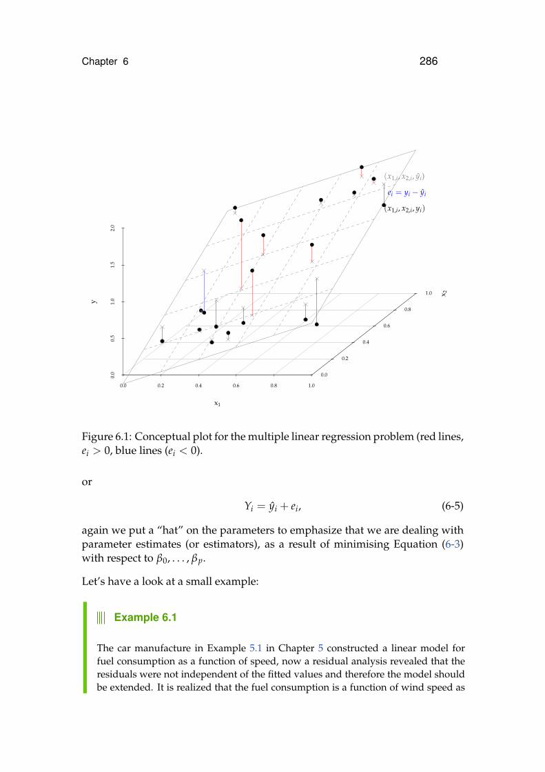
Chapter 6 286
0.0 0.2 0.4 0.6 0.8 1.0
0.0
0.5
1.0
1.5
2.0
0.0
0.2
0.4
0.6
0.8
1.0
x1
x 2
y
(x1,i, x2,i, yi)
(x1,i, x2,i, yi)
ei = yi − yi
Figure 6.1: Conceptual plot for the multiple linear regression problem (red lines,ei > 0, blue lines (ei < 0).
or
Yi = yi + ei, (6-5)
again we put a “hat” on the parameters to emphasize that we are dealing withparameter estimates (or estimators), as a result of minimising Equation (6-3)with respect to β0, . . . , βp.
Let’s have a look at a small example:
Example 6.1
The car manufacture in Example 5.1 in Chapter 5 constructed a linear model forfuel consumption as a function of speed, now a residual analysis revealed that theresiduals were not independent of the fitted values and therefore the model shouldbe extended. It is realized that the fuel consumption is a function of wind speed as

Chapter 6 6.1 PARAMETER ESTIMATION 287
well as the speed of the car, and a new model could be formulated as
Yi = β0 + β1x1,i + β2x2,i + ε i (6-6)
where x1,i is the speed, and x2,i is the wind speed (relative to the car). Anotherpossibility is that the model should in fact not be linear in the speed, but ratherquadratic
Yi = β0 + β1x1,i + β2x21,i + ε i (6-7)
= β0 + β1x1,i + β2x2,i + ε i, (6-8)
where x2,i is now the squared speed. Both models ((6-6) and (6-7)) are linear in theparameters (β0, β1, β2).
The example above illustrate that linearity refers to linearity in the parameters,not the regressors. E.g. the model
Yi = β0 + β2 log(xi) + εi, (6-9)
is a linear model, while
Yi = β0 + log(xi + β2) + εi, (6-10)
is not a linear model.
6.1 Parameter estimation
Just as in the case of simple linear regression the optimal parameters are theparameters that minimize the residual sum of squares (RSS), this is equivalentto equating the partial derivatives of RSS (Equation (6-3)) with zero, i.e.
∂RSS∂β j
= 0; j = 0, 1, . . . , p, (6-11)
which will give us p + 1 equations (the partial derivatives) in p + 1 unknowns(the parameters)
2n
∑i=1
[yi − (β0 + β1x1,i + · · ·+ βpxp,i)
]= 0, (6-12)
2n
∑i=1
[yi − (β0 + β1x1,i + · · ·+ βpxp,i)x1,i
]= 0, (6-13)
...
2n
∑i=1
[yi − (β0 + β1x1,i + · · ·+ βpxp,i)xp,i
]= 0, (6-14)

Chapter 6 6.1 PARAMETER ESTIMATION 288
the Equations (6-12)-(6-14) are referred to as the normal equations, and as wecan see these are a system of linear equations and thus best solved by methodsof linear algebra. The matrix formulation is covered in Section 6.6, but for nowwe will just assume that R is able to solve the normal equations and give thecorrect parameter estimates, standard errors for the parameter estimates, etc.
When the εi’s are independent identically normally distributed, we can con-struct tests for the individual parameters, assuming we know the parameterestimates and their standard errors:
Theorem 6.2 Hypothesis tests and confidence intervals
Suppose the we are given parameter estimates (β0, . . . , βp) and their corre-sponding standard errors (σβ0 , . . . , σβp), then under the null hypothesis
H0,i : βi = β0,i, (6-15)
the t-statistic
Ti =βi − β0,i
σβi
, (6-16)
will follow the t-distribution with n− (p + 1) degrees of freedom, and hy-pothesis testing and confidence intervals should be based on this distribu-tion. Further, a central estimate for the residual variance is
σ2 =RSS(β0, . . . , βp)
n− (p + 1). (6-17)
The interpretation of multiple linear regression in R is illustrated in the follow-ing example:
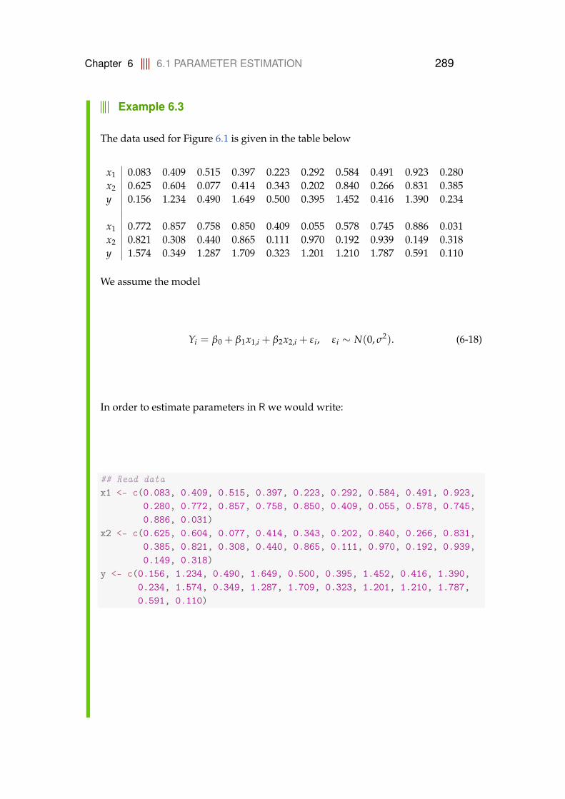
Chapter 6 6.1 PARAMETER ESTIMATION 289
Example 6.3
The data used for Figure 6.1 is given in the table below
x1 0.083 0.409 0.515 0.397 0.223 0.292 0.584 0.491 0.923 0.280x2 0.625 0.604 0.077 0.414 0.343 0.202 0.840 0.266 0.831 0.385y 0.156 1.234 0.490 1.649 0.500 0.395 1.452 0.416 1.390 0.234
x1 0.772 0.857 0.758 0.850 0.409 0.055 0.578 0.745 0.886 0.031x2 0.821 0.308 0.440 0.865 0.111 0.970 0.192 0.939 0.149 0.318y 1.574 0.349 1.287 1.709 0.323 1.201 1.210 1.787 0.591 0.110
We assume the model
Yi = β0 + β1x1,i + β2x2,i + ε i, ε i ∼ N(0, σ2). (6-18)
In order to estimate parameters in R we would write:
## Read datax1 <- c(0.083, 0.409, 0.515, 0.397, 0.223, 0.292, 0.584, 0.491, 0.923,
0.280, 0.772, 0.857, 0.758, 0.850, 0.409, 0.055, 0.578, 0.745,0.886, 0.031)
x2 <- c(0.625, 0.604, 0.077, 0.414, 0.343, 0.202, 0.840, 0.266, 0.831,0.385, 0.821, 0.308, 0.440, 0.865, 0.111, 0.970, 0.192, 0.939,0.149, 0.318)
y <- c(0.156, 1.234, 0.490, 1.649, 0.500, 0.395, 1.452, 0.416, 1.390,0.234, 1.574, 0.349, 1.287, 1.709, 0.323, 1.201, 1.210, 1.787,0.591, 0.110)
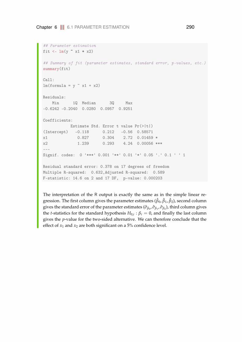
Chapter 6 6.1 PARAMETER ESTIMATION 290
## Parameter estimationfit <- lm(y ~ x1 + x2)
## Summary of fit (parameter estimates, standard error, p-values, etc.)summary(fit)
Call:lm(formula = y ~ x1 + x2)
Residuals:Min 1Q Median 3Q Max
-0.6242 -0.2040 0.0280 0.0957 0.9251
Coefficients:Estimate Std. Error t value Pr(>|t|)
(Intercept) -0.118 0.212 -0.56 0.58571x1 0.827 0.304 2.72 0.01459 *x2 1.239 0.293 4.24 0.00056 ***---Signif. codes: 0 '***' 0.001 '**' 0.01 '*' 0.05 '.' 0.1 ' ' 1
Residual standard error: 0.378 on 17 degrees of freedomMultiple R-squared: 0.632,Adjusted R-squared: 0.589F-statistic: 14.6 on 2 and 17 DF, p-value: 0.000203
The interpretation of the R output is exactly the same as in the simple linear re-gression. The first column gives the parameter estimates (β0, β1, β2), second columngives the standard error of the parameter estimates (σβ0 , σβ1 , σβ2), third column givesthe t-statistics for the standard hypothesis H0,i : βi = 0, and finally the last columngives the p-value for the two-sided alternative. We can therefore conclude that theeffect of x1 and x2 are both significant on a 5% confidence level.

Chapter 6 6.1 PARAMETER ESTIMATION 291
Method 6.4 Level α t-tests for parameters
1. Formulate the null hypothesis: H0,i : βi = β0,i, and the alternative hy-pothesis H1,i : βi 6= β0,i
2. Compute the test statistic tobs,βi =βi−β0,i
σβi
3. Compute the evidence against the null hypothesis
p-valuei = 2P(T > |tobs,βi |) (6-19)
4. If the p-valuei < α reject H0,i, otherwise accept H0,i
In many situations we will be more interested in quantifying the uncertainty ofthe parameter estimates rather than testing a specific hypothesis. This is usuallygiven in the form of confidence intervals for the parameters:
Method 6.5 Parameter confidence intervals
(1− α) confidence interval for βi is given by
βi ± t1−α/2 σβi , (6-20)
where t1−α/2 is the (1 − α/2)-quantile of a t-distribution with n − (p + 1)degrees of freedom.
Remark 6.6 (On finding βi and σβiin methods 6.4 and 6.5)
In Chapter 5 we were able to formulate the exact formulas for βi and σβi, in
a multiple linear regression setting we simply use R (summary(fit)), to findthese values.The explicit formulas are however given in the matrix formulation of thelinear regression problem in Section 6.6.

Chapter 6 6.1 PARAMETER ESTIMATION 292
Example 6.7
For our example the 95% confidence intervals become (t1−α/2 = 2.110)
Iβ0 = −0.118± 2.110 · 0.212, (6-21)
Iβ1 = 0.827± 2.110 · 0.304, (6-22)
Iβ2 = 1.239± 2.110 · 0.293, (6-23)
or in R (for β0):
-0.118+c(-1,1)*qt(0.975,df=17)*0.212
[1] -0.5653 0.3293
or directly in R (for β0, β1, and β2):
confint(fit, level = 0.95)
2.5 % 97.5 %(Intercept) -0.5643 0.329x1 0.1854 1.470x2 0.6220 1.857
The examples above illustrates how we can construct confidence intervals forthe parameters and test hypotheses without having to implement the actualestimation ourselves.
6.1.1 Confidence and prediction intervals for the line
Just as for the simple linear regression model we will often be interested in pre-diction of future outcome of an experiment, and as usual we will be interestedin quantifying the uncertainty of such an experiment. The expected value of anew experiment (with x1 = x1,new, . . . , xp = xp,new) is
ynew = β0 + β1x1,new + . . . + βpxp,new. (6-24)
In order to quantify the uncertainty of this estimate we need to calculate thevariance of ynew, in Section 5.3 we saw that this variance is a function of: 1) thevariance of the parameters, 2) the covariance between the parameters, and 3)xnew. This is also true in the multiple linear regression case, except that xnew is
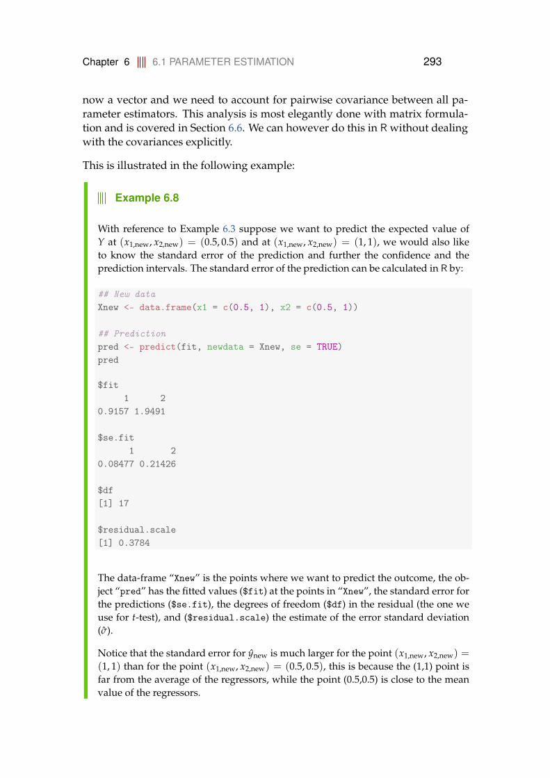
Chapter 6 6.1 PARAMETER ESTIMATION 293
now a vector and we need to account for pairwise covariance between all pa-rameter estimators. This analysis is most elegantly done with matrix formula-tion and is covered in Section 6.6. We can however do this in R without dealingwith the covariances explicitly.
This is illustrated in the following example:
Example 6.8
With reference to Example 6.3 suppose we want to predict the expected value ofY at (x1,new, x2,new) = (0.5, 0.5) and at (x1,new, x2,new) = (1, 1), we would also liketo know the standard error of the prediction and further the confidence and theprediction intervals. The standard error of the prediction can be calculated in R by:
## New dataXnew <- data.frame(x1 = c(0.5, 1), x2 = c(0.5, 1))
## Predictionpred <- predict(fit, newdata = Xnew, se = TRUE)pred
$fit1 2
0.9157 1.9491
$se.fit1 2
0.08477 0.21426
$df[1] 17
$residual.scale[1] 0.3784
The data-frame “Xnew” is the points where we want to predict the outcome, the ob-ject “pred” has the fitted values ($fit) at the points in “Xnew”, the standard error forthe predictions ($se.fit), the degrees of freedom ($df) in the residual (the one weuse for t-test), and ($residual.scale) the estimate of the error standard deviation(σ).
Notice that the standard error for ynew is much larger for the point (x1,new, x2,new) =
(1, 1) than for the point (x1,new, x2,new) = (0.5, 0.5), this is because the (1,1) point isfar from the average of the regressors, while the point (0.5,0.5) is close to the meanvalue of the regressors.
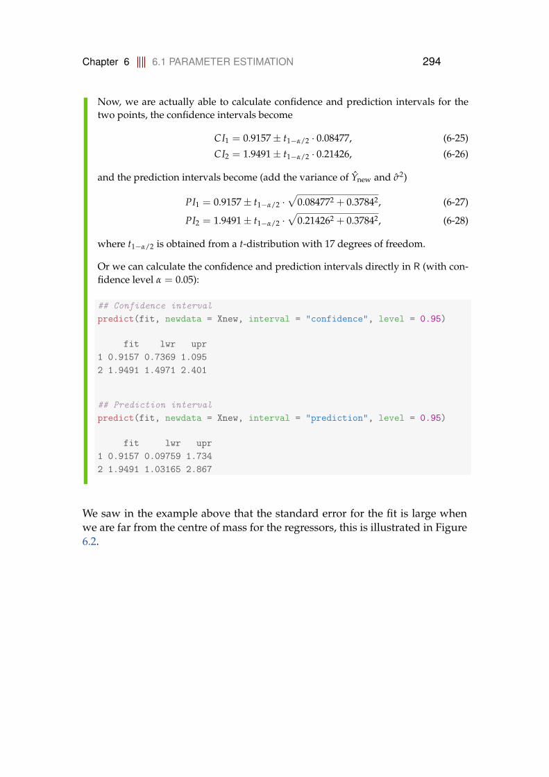
Chapter 6 6.1 PARAMETER ESTIMATION 294
Now, we are actually able to calculate confidence and prediction intervals for thetwo points, the confidence intervals become
CI1 = 0.9157± t1−α/2 · 0.08477, (6-25)
CI2 = 1.9491± t1−α/2 · 0.21426, (6-26)
and the prediction intervals become (add the variance of Ynew and σ2)
PI1 = 0.9157± t1−α/2 ·√
0.084772 + 0.37842, (6-27)
PI2 = 1.9491± t1−α/2 ·√
0.214262 + 0.37842, (6-28)
where t1−α/2 is obtained from a t-distribution with 17 degrees of freedom.
Or we can calculate the confidence and prediction intervals directly in R (with con-fidence level α = 0.05):
## Confidence intervalpredict(fit, newdata = Xnew, interval = "confidence", level = 0.95)
fit lwr upr1 0.9157 0.7369 1.0952 1.9491 1.4971 2.401
## Prediction intervalpredict(fit, newdata = Xnew, interval = "prediction", level = 0.95)
fit lwr upr1 0.9157 0.09759 1.7342 1.9491 1.03165 2.867
We saw in the example above that the standard error for the fit is large whenwe are far from the centre of mass for the regressors, this is illustrated in Figure6.2.

Chapter 6 6.1 PARAMETER ESTIMATION 295
0.0 0.2 0.4 0.6 0.8 1.0
0.0
0.1
0.2
0.3
0.4
0.5
0.0
0.2
0.4
0.6
0.8
1.0
x1
x 2
σy
Figure 6.2: Standard error for ynew (blue surface) and standard error for ynew(red surface).

Chapter 6 6.2 CURVILINEAR REGRESSION 296
Method 6.9 Intervals for the line (by R)
The (1-α) confidence and prediction intervals for the line β0 + β1x1,new +· · ·+ βpxp,new are calculated in R by
## Confidence intervalpredict(fit, newdata=Xnew, interval="confidence", level=1-alpha)## Prediction intervalpredict(fit, newdata=Xnew, interval="prediction", level=1-alpha)
Remark 6.10
Explicit formulas for confidence and prediction intervals are given in Section6.6.
6.2 Curvilinear regression
Suppose we are given pairs of values of x and y and there seems to be informa-tion in x about y, but the relation is clearly non-linear
Yi = f (xi) + εi, εi ∼ N(0, σ2), (6-29)
and the non-linear function f (x) is unknown to us. The methods we have dis-cussed don’t apply for non-linear functions, and even if we could do non-linearregression we would not know which function to insert. We do however knowfrom elementary calculus that any function can be approximated by its Taylorseries
f (x) ≈ f (0) + f ′(0) · x +f ′′(0)
2x2 + · · ·+ f (p)(0)
p!xp, (6-30)
now replace the Taylor series coefficients(
f (j)(0)j!
)by β j and insert (6-30) in
(6-29) to get
Yi = β0 + β1x + β2x2 + · · ·+ βpxp + εi
= β0 + β1x1 + β2x2 + · · ·+ βpxp + εi,(6-31)
where xj = xj, we refer to this method as curvilinear regression. The method isillustrated in the following example:

Chapter 6 6.2 CURVILINEAR REGRESSION 297
Example 6.11 Simulation of non-linear model
We simulate the following model
Yi = sin(πxi) + ε i, ε i ∼ N(0, 0.12), (6-32)
with x ∈ [0, 1] by:
n <- 200x <- runif(n)y <- sin(pi*x) + rnorm(n,sd=0.1)
Yi is a non-linear function of x but lets try to estimate parameters in the simple linearregression model
Yi = β0 + β1xi + ε i, ε i ∼ N(0, σ2), (6-33)
and find the 95% confidence interval for the parameters:
fit1 <- lm(y ~ x)confint(fit1)
2.5 % 97.5 %(Intercept) 0.5737 0.7544x -0.1960 0.1251
We see that the 95% confidence interval for β1 covers zero, and we can thereforenot reject the null hypothesis that β1 is zero. Now include a quadratic term in x1 toapproximate the non-linear function by the model
Yi = β0 + β1xi + β2x2i + ε i, ε i ∼ N(0, σ2), (6-34)
x1 <- x; x2 <- x^2fit2 <- lm(y ~ x1 + x2)confint(fit2)
2.5 % 97.5 %(Intercept) -0.0906 -0.005303x1 3.9858 4.381327x2 -4.3823 -4.001747
Now we see that all parameters are significantly different from zero on a 5% confi-dence level. The plot below shows the residuals for the two models as a function ofthe fitted values:

Chapter 6 6.2 CURVILINEAR REGRESSION 298
0.630 0.640 0.650 0.660
-0.6
-0.2
0.2
0.4
fit1$fitted.values
fit1$
resi
dual
s
0.0 0.2 0.4 0.6 0.8 1.0
-0.3
-0.1
0.1
0.2
0.3
fit2$fitted.values
fit2$
resi
dual
sIt is clear that including the second order term removed most, if not all, systematicdependence in the residuals. Also looking at the fitted values together with theactual values shows that we have a much better model when including the secondorder term (red line):
0.0 0.2 0.4 0.6 0.8 1.0
0.0
0.2
0.4
0.6
0.8
1.0
x
y
Remark 6.12
In general one should be careful when extrapolation models into areaswhere there is no data, and this is in particular true when we use curvilinearregression.
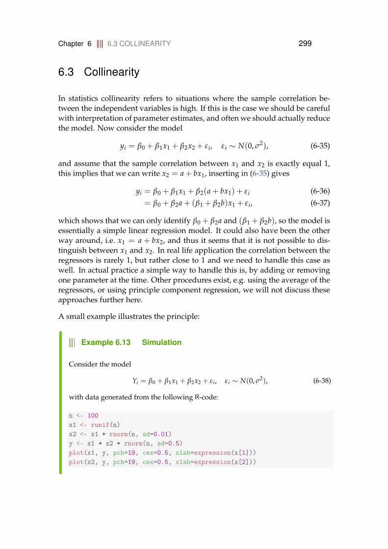
Chapter 6 6.3 COLLINEARITY 299
6.3 Collinearity
In statistics collinearity refers to situations where the sample correlation be-tween the independent variables is high. If this is the case we should be carefulwith interpretation of parameter estimates, and often we should actually reducethe model. Now consider the model
yi = β0 + β1x1 + β2x2 + εi, εi ∼ N(0, σ2), (6-35)
and assume that the sample correlation between x1 and x2 is exactly equal 1,this implies that we can write x2 = a + bx1, inserting in (6-35) gives
yi = β0 + β1x1 + β2(a + bx1) + εi (6-36)= β0 + β2a + (β1 + β2b)x1 + εi, (6-37)
which shows that we can only identify β0 + β2a and (β1 + β2b), so the model isessentially a simple linear regression model. It could also have been the otherway around, i.e. x1 = a + bx2, and thus it seems that it is not possible to dis-tinguish between x1 and x2. In real life application the correlation between theregressors is rarely 1, but rather close to 1 and we need to handle this case aswell. In actual practice a simple way to handle this is, by adding or removingone parameter at the time. Other procedures exist, e.g. using the average of theregressors, or using principle component regression, we will not discuss theseapproaches further here.
A small example illustrates the principle:
Example 6.13 Simulation
Consider the model
Yi = β0 + β1x1 + β2x2 + ε i, ε i ∼ N(0, σ2), (6-38)
with data generated from the following R-code:
n <- 100x1 <- runif(n)x2 <- x1 + rnorm(n, sd=0.01)y <- x1 + x2 + rnorm(n, sd=0.5)plot(x1, y, pch=19, cex=0.5, xlab=expression(x[1]))plot(x2, y, pch=19, cex=0.5, xlab=expression(x[2]))

Chapter 6 6.3 COLLINEARITY 300
0.0 0.2 0.4 0.6 0.8 1.0
01
23
x1
y
0.0 0.2 0.4 0.6 0.8 1.0
01
23
x2
yClearly, both x1 and x2 contain information about y, but our usual linear regressiongives:
confint(lm(y ~ x1 + x2))
2.5 % 97.5 %(Intercept) -0.3453 0.07124x1 -14.9270 5.98682x2 -3.6745 17.20468
we see that none of the parameters are significant (on a 5% level), but if we removex1 (this is the one with the highest p-value) from the model we get:
summary(lm(y ~ x2))
Call:lm(formula = y ~ x2)
Residuals:Min 1Q Median 3Q Max
-1.2229 -0.3025 0.0025 0.2641 1.7649
Coefficients:Estimate Std. Error t value Pr(>|t|)
(Intercept) -0.140 0.105 -1.33 0.19x2 2.305 0.194 11.86 <2e-16 ***---Signif. codes: 0 '***' 0.001 '**' 0.01 '*' 0.05 '.' 0.1 ' ' 1
Residual standard error: 0.502 on 98 degrees of freedomMultiple R-squared: 0.589,Adjusted R-squared: 0.585F-statistic: 141 on 1 and 98 DF, p-value: <2e-16
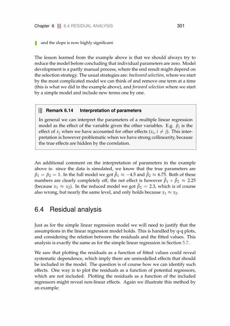
Chapter 6 6.4 RESIDUAL ANALYSIS 301
and the slope is now highly significant.
The lesson learned from the example above is that we should always try toreduce the model before concluding that individual parameters are zero. Modeldevelopment is a partly manual process, where the end result might depend onthe selection strategy. The usual strategies are: backward selection, where we startby the most complicated model we can think of and remove one term at a time(this is what we did in the example above), and forward selection where we startby a simple model and include new terms one by one.
Remark 6.14 Interpretation of parameters
In general we can interpret the parameters of a multiple linear regressionmodel as the effect of the variable given the other variables. E.g. β j is theeffect of xj when we have accounted for other effects (xi, i 6= j). This inter-pretation is however problematic when we have strong collinearity, becausethe true effects are hidden by the correlation.
An additional comment on the interpretation of parameters in the exampleabove is: since the data is simulated, we know that the true parameters areβ1 = β2 = 1. In the full model we got β1 ≈ −4.5 and β2 ≈ 6.75. Both of thesenumbers are clearly completely off, the net effect is however β1 + β2 ≈ 2.25(because x1 ≈ x2). In the reduced model we got β2 = 2.3, which is of coursealso wrong, but nearly the same level, and only holds because x1 ≈ x2.
6.4 Residual analysis
Just as for the simple linear regression model we will need to justify that theassumptions in the linear regression model holds. This is handled by q-q plots,and considering the relation between the residuals and the fitted values. Thisanalysis is exactly the same as for the simple linear regression in Section 5.7.
We saw that plotting the residuals as a function of fitted values could revealsystematic dependence, which imply there are unmodelled effects that shouldbe included in the model. The question is of course how we can identify sucheffects. One way is to plot the residuals as a function of potential regressors,which are not included. Plotting the residuals as a function of the includedregressors might reveal non-linear effects. Again we illustrate this method byan example:
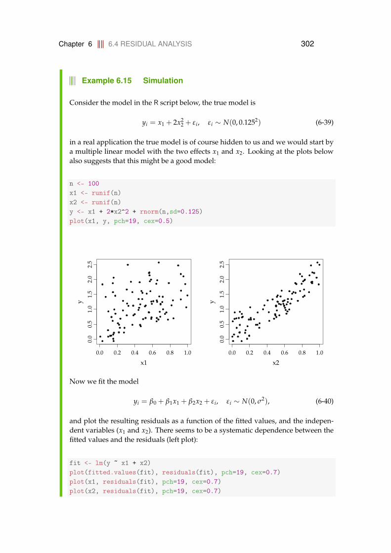
Chapter 6 6.4 RESIDUAL ANALYSIS 302
Example 6.15 Simulation
Consider the model in the R script below, the true model is
yi = x1 + 2x22 + ε i, ε i ∼ N(0, 0.1252) (6-39)
in a real application the true model is of course hidden to us and we would start bya multiple linear model with the two effects x1 and x2. Looking at the plots belowalso suggests that this might be a good model:
n <- 100x1 <- runif(n)x2 <- runif(n)y <- x1 + 2*x2^2 + rnorm(n,sd=0.125)plot(x1, y, pch=19, cex=0.5)
0.0 0.2 0.4 0.6 0.8 1.0
0.0
0.5
1.0
1.5
2.0
2.5
x1
y
0.0 0.2 0.4 0.6 0.8 1.0
0.0
0.5
1.0
1.5
2.0
2.5
x2
y
Now we fit the model
yi = β0 + β1x1 + β2x2 + ε i, ε i ∼ N(0, σ2), (6-40)
and plot the resulting residuals as a function of the fitted values, and the indepen-dent variables (x1 and x2). There seems to be a systematic dependence between thefitted values and the residuals (left plot):
fit <- lm(y ~ x1 + x2)plot(fitted.values(fit), residuals(fit), pch=19, cex=0.7)plot(x1, residuals(fit), pch=19, cex=0.7)plot(x2, residuals(fit), pch=19, cex=0.7)
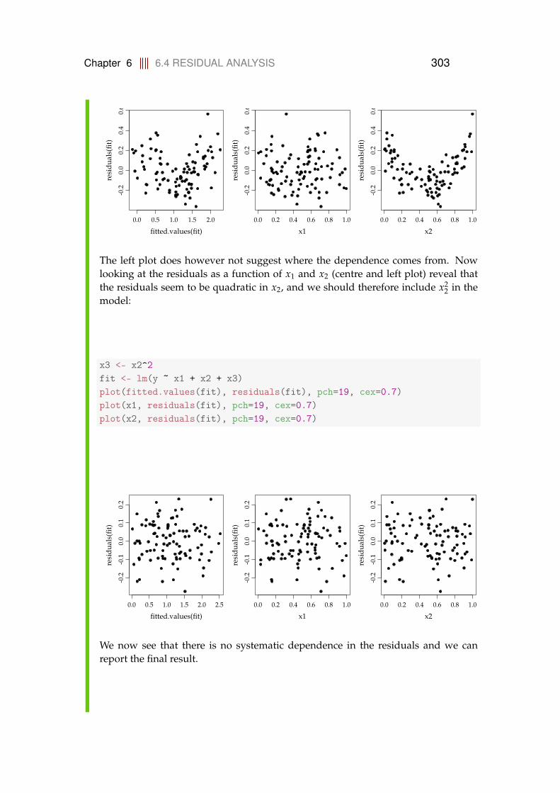
Chapter 6 6.4 RESIDUAL ANALYSIS 303
0.0 0.5 1.0 1.5 2.0
-0.2
0.0
0.2
0.4
0.6
fitted.values(fit)
resi
dual
s(fit
)
0.0 0.2 0.4 0.6 0.8 1.0
-0.2
0.0
0.2
0.4
0.6
x1re
sidu
als(
fit)
0.0 0.2 0.4 0.6 0.8 1.0
-0.2
0.0
0.2
0.4
0.6
x2
resi
dual
s(fit
)
The left plot does however not suggest where the dependence comes from. Nowlooking at the residuals as a function of x1 and x2 (centre and left plot) reveal thatthe residuals seem to be quadratic in x2, and we should therefore include x2
2 in themodel:
x3 <- x2^2fit <- lm(y ~ x1 + x2 + x3)plot(fitted.values(fit), residuals(fit), pch=19, cex=0.7)plot(x1, residuals(fit), pch=19, cex=0.7)plot(x2, residuals(fit), pch=19, cex=0.7)
0.0 0.5 1.0 1.5 2.0 2.5
-0.2
-0.1
0.0
0.1
0.2
fitted.values(fit)
resi
dual
s(fit
)
0.0 0.2 0.4 0.6 0.8 1.0
-0.2
-0.1
0.0
0.1
0.2
x1
resi
dual
s(fit
)
0.0 0.2 0.4 0.6 0.8 1.0
-0.2
-0.1
0.0
0.1
0.2
x2
resi
dual
s(fit
)
We now see that there is no systematic dependence in the residuals and we canreport the final result.

Chapter 6 6.5 LINEAR REGRESSION IN R 304
summary(fit)
Call:lm(formula = y ~ x1 + x2 + x3)
Residuals:Min 1Q Median 3Q Max
-0.27486 -0.07353 -0.00098 0.07630 0.23112
Coefficients:Estimate Std. Error t value Pr(>|t|)
(Intercept) -0.000979 0.032200 -0.03 0.98x1 0.998212 0.042055 23.74 <2e-16 ***x2 0.087010 0.138613 0.63 0.53x3 1.859060 0.140499 13.23 <2e-16 ***---Signif. codes: 0 '***' 0.001 '**' 0.01 '*' 0.05 '.' 0.1 ' ' 1
Residual standard error: 0.107 on 96 degrees of freedomMultiple R-squared: 0.972,Adjusted R-squared: 0.972F-statistic: 1.13e+03 on 3 and 96 DF, p-value: <2e-16
Now we can actually see that we find parameter values close to the true ones, furtherwe might actually exclude x2 (while keeping x2
2) and the intercept from the model,since they are not significantly different from zero.
6.5 Linear regression in R
Method 6.16 below gives a practical summary of Chapter 5 and 6 with refer-ences to the applied R-functions.
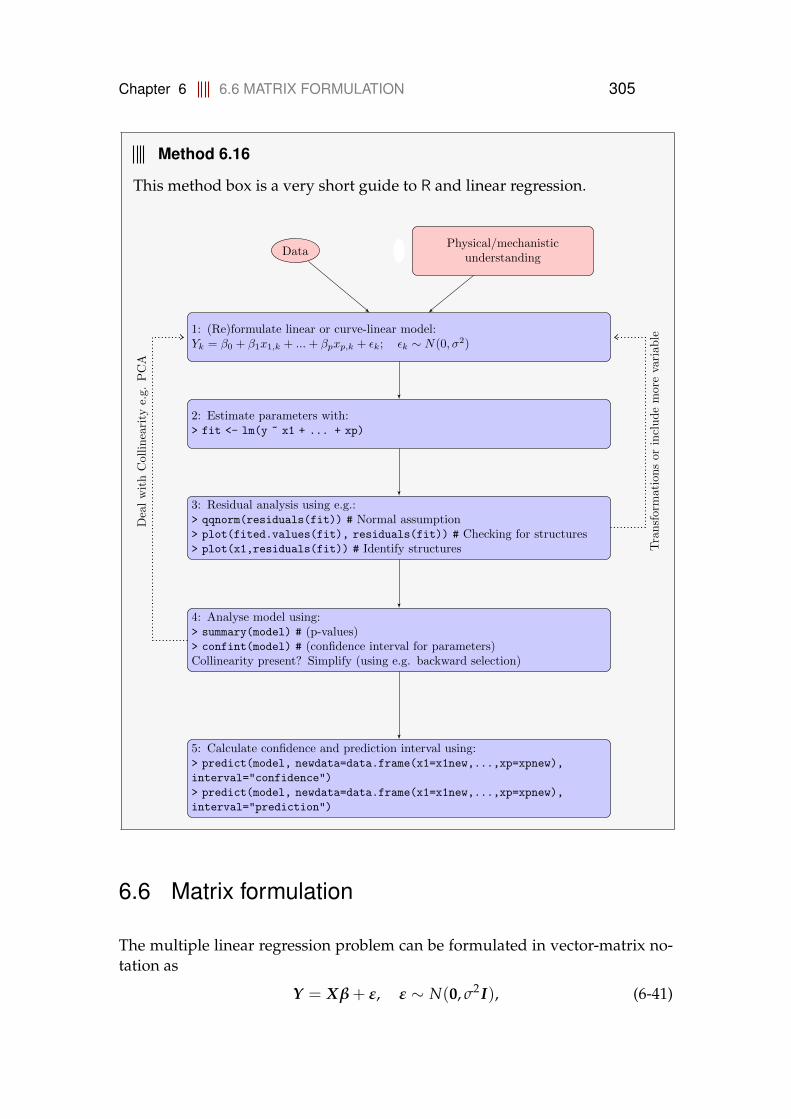
Chapter 6 6.6 MATRIX FORMULATION 305
Method 6.16
This method box is a very short guide to R and linear regression.
DataPhysical/mechanistic
understanding
1: (Re)formulate linear or curve-linear model:Yk = β0 + β1x1,k + ...+ βpxp,k + εk; εk ∼ N(0, σ2)
2: Estimate parameters with:> fit <- lm(y ~ x1 + ... + xp)
3: Residual analysis using e.g.:> qqnorm(residuals(fit)) # Normal assumption> plot(fited.values(fit), residuals(fit)) # Checking for structures> plot(x1,residuals(fit)) # Identify structures
4: Analyse model using:> summary(model) # (p-values)> confint(model) # (confidence interval for parameters)Collinearity present? Simplify (using e.g. backward selection)
5: Calculate confidence and prediction interval using:> predict(model, newdata=data.frame(x1=x1new,...,xp=xpnew),
interval="confidence")
> predict(model, newdata=data.frame(x1=x1new,...,xp=xpnew),
interval="prediction")
Tra
nsf
orm
atio
ns
orin
clude
more
vari
able
Dea
lw
ith
Col
linea
rity
e.g.
PC
A
6.6 Matrix formulation
The multiple linear regression problem can be formulated in vector-matrix no-tation as
Y = Xβ + ε, ε ∼ N(0, σ2I), (6-41)
Chapter 6 6.6 MATRIX FORMULATION 306
or
Y1...
Yn
=
1 x1,1 · · · xp,1...
......
1 x1,n · · · xp,n
β0...
βp
+
ε1...
εn
, εi ∼ N(0, σ2). (6-42)
Notice, that the formulation in (6-41) is exactly the same as we saw in Section5.5.
The residual sum of squares are calculated by
RSS = εTε = (y− Xβ)T(y− Xβ), (6-43)
and the parameter estimates are given by:
Theorem 6.17
The estimators of the parameters in the simple linear regression model aregiven by
β = (XTX)−1XTY , (6-44)
and the covariance matrix of the estimates is
V[β] = σ2(XTX)−1, (6-45)
and central estimate for the residual variance is
σ2 =RSS
n− (p + 1). (6-46)
The proof of this theorem follows the exact same arguments as the matrix for-mulation of the simple linear regression model in Chapter 5 and hence it isomitted here.
Marginal tests (H0 : βi = βi,0) can also in the multiple linear regression case beconstructed by
βi − βi,0√(Σβ)ii
∼ t(n− (p + 1)). (6-47)
Chapter 6 6.6 MATRIX FORMULATION 307
6.6.1 Confidence and prediction intervals for the line
Now suppose that we want to make a prediction at a new point
xnew = [1, x1,new, . . . , xp,new],
in order to construct confidence and prediction intervals we calculate the vari-ance of Ynew
V(Ynew) = V(xnewβ)
= xnew V(β)xTnew
= σ2xnew(XTX)−1xTnew,
(6-48)
in practice we will of course replace σ2 with its estimate (σ2), and hence usequantile of the appropriate t-distribution (and standard errors rather than vari-ances) to calculate confidence intervals. The variance of a single prediction iscalculated by
V(Ynew) = V(xnewβ + εnew)
= xnew V(β)xTnew + σ2
= σ2(1 + xnew(XTX)−1xTnew).
(6-49)
The calculations above illustrate that the derivations of variances are relativelysimple, when we formulate our model in the matrix-vector notation.

Chapter 6 6.7 EXERCISES 308
6.7 Exercises
Exercise 6.1 Nitrate concentration
In order to analyze the effect of reducing nitrate loading in a Danish fjord, it wasdecided to formulate a linear model that describes the nitrate concentration inthe fjord as a function of nitrate loading, it was further decided to correct forfresh water runoff. The resulting model was
Yi = β0 + β1x1,i + β2x2,i + εi, εi ∼ N(0, σ2), (6-50)
where Yi is the natural logarithm of nitrate concentration, x1,i is the naturallogarithm of nitrate loading, and x2,i is the natural logarithm of fresh waterrun off.
a) Which of the following statements are assumed fulfilled in the usual mul-tiple linear regression model?
1 ) εi = 0 for all i = 1, ..., n, and β j follows a normal distribution
2 ) E[x1] = E[x2] = 0 and V[εi] = β21
3 ) E[εi] = 0 and V[εi] = β21
4 ) εi is normally distributed with constant variance, and εi and ε j areindependent for i 6= j
5 ) εi = 0 for all i = 1, ..., n, and xj follows a normal distribution forj = {1, 2}
The parameters in the model were estimated in R and the following results areavailable (slightly modified output from summary):
> summary(lm(y ~ x1 + x2))
Call:lm(formula = y ~ x1 + x2)
Coefficients:Estimate Std. Error t value Pr(>|t|)
(Intercept) -2.36500 0.22184 -10.661 < 2e-16x1 0.47621 0.06169 7.720 3.25e-13x2 0.08269 0.06977 1.185 0.237
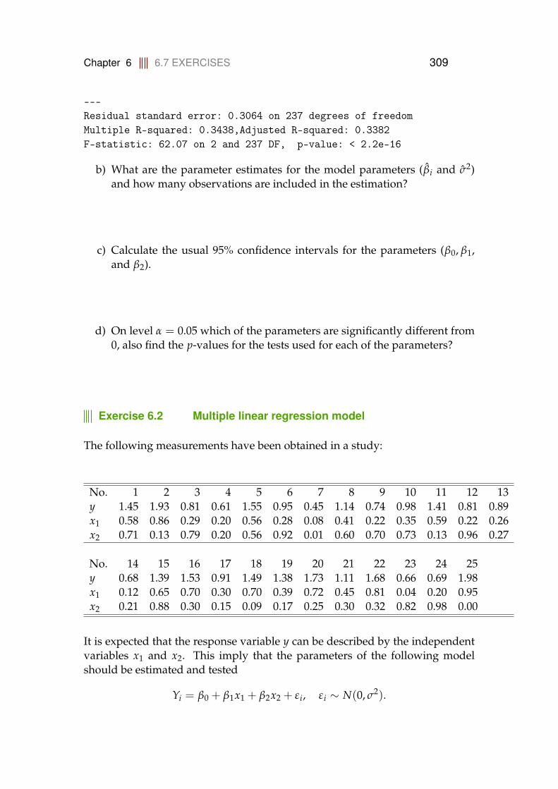
Chapter 6 6.7 EXERCISES 309
---Residual standard error: 0.3064 on 237 degrees of freedomMultiple R-squared: 0.3438,Adjusted R-squared: 0.3382F-statistic: 62.07 on 2 and 237 DF, p-value: < 2.2e-16
b) What are the parameter estimates for the model parameters (βi and σ2)and how many observations are included in the estimation?
c) Calculate the usual 95% confidence intervals for the parameters (β0, β1,and β2).
d) On level α = 0.05 which of the parameters are significantly different from0, also find the p-values for the tests used for each of the parameters?
Exercise 6.2 Multiple linear regression model
The following measurements have been obtained in a study:
No. 1 2 3 4 5 6 7 8 9 10 11 12 13y 1.45 1.93 0.81 0.61 1.55 0.95 0.45 1.14 0.74 0.98 1.41 0.81 0.89x1 0.58 0.86 0.29 0.20 0.56 0.28 0.08 0.41 0.22 0.35 0.59 0.22 0.26x2 0.71 0.13 0.79 0.20 0.56 0.92 0.01 0.60 0.70 0.73 0.13 0.96 0.27
No. 14 15 16 17 18 19 20 21 22 23 24 25y 0.68 1.39 1.53 0.91 1.49 1.38 1.73 1.11 1.68 0.66 0.69 1.98x1 0.12 0.65 0.70 0.30 0.70 0.39 0.72 0.45 0.81 0.04 0.20 0.95x2 0.21 0.88 0.30 0.15 0.09 0.17 0.25 0.30 0.32 0.82 0.98 0.00
It is expected that the response variable y can be described by the independentvariables x1 and x2. This imply that the parameters of the following modelshould be estimated and tested
Yi = β0 + β1x1 + β2x2 + εi, εi ∼ N(0, σ2).

Chapter 6 6.7 EXERCISES 310
a) Calculate the parameter estimates (β0, β1, β2, and σ2), in addition find theusual 95% confidence intervals for β0, β1, and β2.You can copy the following lines to R to load the data:
D <- data.frame(x1=c(0.58, 0.86, 0.29, 0.20, 0.56, 0.28, 0.08, 0.41, 0.22, 0.35,
0.59, 0.22, 0.26, 0.12, 0.65, 0.70, 0.30, 0.70, 0.39, 0.72,0.45, 0.81, 0.04, 0.20, 0.95),
x2=c(0.71, 0.13, 0.79, 0.20, 0.56, 0.92, 0.01, 0.60, 0.70, 0.73,0.13, 0.96, 0.27, 0.21, 0.88, 0.30, 0.15, 0.09, 0.17, 0.25,0.30, 0.32, 0.82, 0.98, 0.00),
y=c(1.45, 1.93, 0.81, 0.61, 1.55, 0.95, 0.45, 1.14, 0.74, 0.98,1.41, 0.81, 0.89, 0.68, 1.39, 1.53, 0.91, 1.49, 1.38, 1.73,1.11, 1.68, 0.66, 0.69, 1.98)
)
b) Still using confidence level α = 0.05 reduce the model if appropriate.
c) Carry out a residual analysis to check that the model assumptions are ful-filled.
d) Make a plot of the fitted line and 95% confidence and prediction intervalsof the line for x1 ∈ [0, 1] (it is assumed that the model was reduced above).
Exercise 6.3 MLR simulation exercise
The following measurements have been obtained in a study:
Nr. 1 2 3 4 5 6 7 8y 9.29 12.67 12.42 0.38 20.77 9.52 2.38 7.46x1 1.00 2.00 3.00 4.00 5.00 6.00 7.00 8.00x2 4.00 12.00 16.00 8.00 32.00 24.00 20.00 28.00
Chapter 6 6.7 EXERCISES 311
a) Plot the observed values of y as a function of x1 and x2. Does it seemreasonable that either x1 or x2 can describe the variation in y?You may copy the following lines into R to load the data
D <- data.frame(y=c(9.29,12.67,12.42,0.38,20.77,9.52,2.38,7.46),x1=c(1.00,2.00,3.00,4.00,5.00,6.00,7.00,8.00),x2=c(4.00,12.00,16.00,8.00,32.00,24.00,20.00,28.00)
)
b) Estimate the parameters for the two models
Yi = β0 + β1x1,i + εi, εi ∼ N(0, σ2),
and
Yi = β0 + β1x2,i + εi, εi ∼ N(0, σ2),
and report the 95% confidence intervals for the parameters. Are any of theparameters significantly different from zero on a 5% confidence level?
c) Estimate the parameters for the model
Yi = β0 + β1x1,i + β2x2,i + εi, εi ∼ (N(0, σ2), (6-51)
and go through the steps of Method 6.16 (use confidence level 0.05 in alltests).
d) Find the standard error for the line, and the confidence and prediction in-tervals for the line for the points (min(x1), min(x2)), (x1, x2), (max(x1), max(x2)).
e) Plot the observed values together with the fitted values (e.g. as a functionof x1).
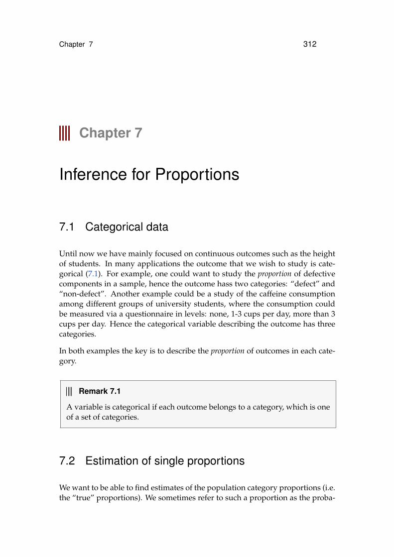
Chapter 7 312
Chapter 7
Inference for Proportions
7.1 Categorical data
Until now we have mainly focused on continuous outcomes such as the heightof students. In many applications the outcome that we wish to study is cate-gorical (7.1). For example, one could want to study the proportion of defectivecomponents in a sample, hence the outcome hass two categories: “defect” and“non-defect”. Another example could be a study of the caffeine consumptionamong different groups of university students, where the consumption couldbe measured via a questionnaire in levels: none, 1-3 cups per day, more than 3cups per day. Hence the categorical variable describing the outcome has threecategories.
In both examples the key is to describe the proportion of outcomes in each cate-gory.
Remark 7.1
A variable is categorical if each outcome belongs to a category, which is oneof a set of categories.
7.2 Estimation of single proportions
We want to be able to find estimates of the population category proportions (i.e.the “true” proportions). We sometimes refer to such a proportion as the proba-
Chapter 7 7.2 ESTIMATION OF SINGLE PROPORTIONS 313
bility of belonging to the category. This is simply because the probability that arandomly sampled observation from the population belongs to the category, isthe proportion of the category in the population.
Example 7.2
In a survey in the US in 2000, 1154 persons answered the question whether theywould be willing to pay more for petrol to help the environment. Of the 1154 par-ticipants 518 answered that they would be willing to do so.
Our best estimate of the proportion of persons willing to pay more (p) is the ob-served proportion of positive answers
p ="Number of positive answers""Total number of participants"
=5181154
= 0.4489.
This means that our best estimate of the proportion of people willing to pay morefor petrol to help the environment is 44.89%.
In the above example we can think of n = 1154 trials, where we each time havea binary outcome (yes or no), occuring with the unknown probability p. Therandom variable X counts the number of times we get a yes to the question,hence X follows a binomial distribution B(n, p) with the probability of observ-ing x successes given by
P(X = x) =(
nx
)px(1− p)n−x. (7-1)
As mentioned in Example 7.2, our best estimate of the unknown p is the pro-portion
p =xn
, p ∈ [0, 1]. (7-2)
From Chapter 2 we know that if X ∼ B(n, p), then
E(X) = np, (7-3)V(X) = np(1− p). (7-4)
This means that
E( p) = E(
Xn
)=
npn
= p, (7-5)
V( p) = V(
Xn
)=
1n2 V(X) =
p(1− p)n
. (7-6)

Chapter 7 7.2 ESTIMATION OF SINGLE PROPORTIONS 314
From Equation (7-5) we see that p is an unbiased estimator of the unknown pand from Equation (7-6) that the standard error (the (sampling) standard devi-
ation) of p is σp =√
p(1−p)n . It is important to quantify the uncertainty of the
calculated estimate using confidence intervals. For large samples, the CentralLimit Theorem gives us that the sample proportion p is well approximated bya normal distribution, and thus a (1− α)100% confidence interval for the pop-ulation proportion p is
p± z1−α/2 σp. (7-7)
However, σp depends on the unknown p, which we do not know. In practicewe will have to estimate the standard error by substituting the unknown p bythe estimate p.
Method 7.3 Proportion estimate and confidence interval
The best estimate of the probability p of belonging to a category (the popu-lation proportion) is the sample proportion
p =xn
, (7-8)
where x is the number of observations in the category and n is the totalnumber of observations.
A large sample (1− α)100% confidence interval for p is given as
p± z1−α/2
√p(1− p)
n. (7-9)
Remark 7.4
As a rule of thumb the normal distribution is a good approximation of thebinomial distrinution if np and n(1− p) are both greater than 15.
Example 7.5
In the figure below we have some examples of binomial distributions. When wereach a size where np ≥ 15 and n(1 − p) ≥ 15 it seems reasonable that the bell-shaped normal distribution will be a good approximation.
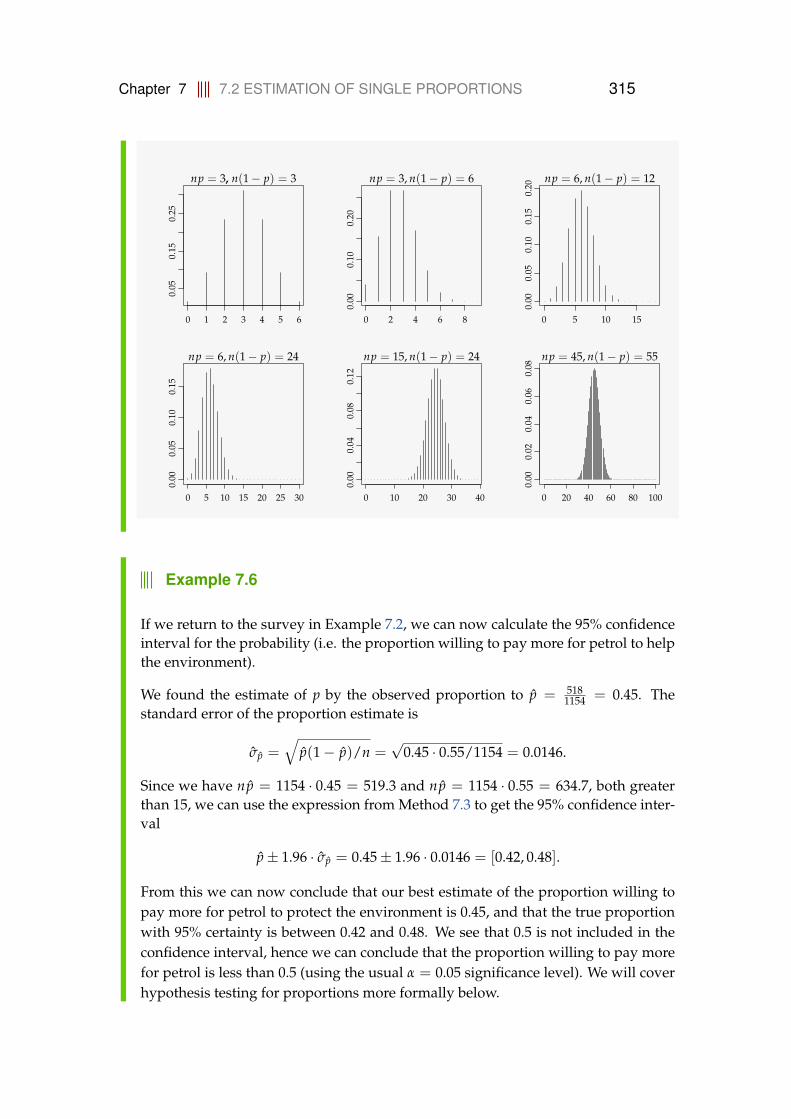
Chapter 7 7.2 ESTIMATION OF SINGLE PROPORTIONS 315
0 1 2 3 4 5 6
0.05
0.15
0.25
np = 3, n(1 − p) = 3
0 2 4 6 8
0.00
0.10
0.20
np = 3, n(1 − p) = 6
0 5 10 15
0.00
0.05
0.10
0.15
0.20
np = 6, n(1 − p) = 12
0 5 10 15 20 25 30
0.00
0.05
0.10
0.15
np = 6, n(1 − p) = 24
0 10 20 30 40
0.00
0.04
0.08
0.12
np = 15, n(1 − p) = 24
0 20 40 60 80 100
0.00
0.02
0.04
0.06
0.08
np = 45, n(1 − p) = 55
Example 7.6
If we return to the survey in Example 7.2, we can now calculate the 95% confidenceinterval for the probability (i.e. the proportion willing to pay more for petrol to helpthe environment).
We found the estimate of p by the observed proportion to p = 5181154 = 0.45. The
standard error of the proportion estimate is
σp =√
p(1− p)/n =√
0.45 · 0.55/1154 = 0.0146.
Since we have np = 1154 · 0.45 = 519.3 and np = 1154 · 0.55 = 634.7, both greaterthan 15, we can use the expression from Method 7.3 to get the 95% confidence inter-val
p± 1.96 · σp = 0.45± 1.96 · 0.0146 = [0.42, 0.48].
From this we can now conclude that our best estimate of the proportion willing topay more for petrol to protect the environment is 0.45, and that the true proportionwith 95% certainty is between 0.42 and 0.48. We see that 0.5 is not included in theconfidence interval, hence we can conclude that the proportion willing to pay morefor petrol is less than 0.5 (using the usual α = 0.05 significance level). We will coverhypothesis testing for proportions more formally below.

Chapter 7 7.2 ESTIMATION OF SINGLE PROPORTIONS 316
Remark 7.7 What about small samples then?
There exist several ways of expressing a valid confidence interval for p insmall sample cases, that is, when either np ≤ 15 or n(1− p) ≤ 15. We men-tion three of these here - only for the last one we give the explicit formula:
Continuity correction
The so-called continuity correction is a general approach to making thebest approximation of discrete probabilities (in this case the binomialprobabilities) using a continuous distribution, (in this case the normaldistribution). We do not give any details here. In fact, a version of sucha correction is the default of the R-function prop.test.
Exact intervals
Probably the most well known of such small sample ways of obtain-ing a valid confidence interval for a proportion is the so-called exactmethod based on actual binomial probabilities rather than a normalapproximation. It is not possible to give a simple formula for theseconfidence limits, and we will not explain the details here, but simplynote that they can be obtained by the R-function binom.test. Thesewill be valid no matter the size of n and p.
“Plus 2”-approach
Finally, a simple approach to a good small sample confidence inter-val for a proportion, will be to us the simple formula given above inMethod 7.3, but applied to x = x + 2 and n = n + 4.
Chapter 7 7.2 ESTIMATION OF SINGLE PROPORTIONS 317
Remark 7.8 Confidence intervals for single proportions in R
In R we can use either the function prop.test or binom.test to find theconfidence interval of a single proportion (and some hypothesis testing in-formation to be described below).
The binom.test uses the exact approach. The prop.test uses a version ofthe continuity correction as default and something yet different again whena continuity correction is not applied (using the option correct=FALSE).
Therefore: none of these (three different) intervals calculated by R coincidesexactly with the formula given in Method 7.3, neither applied to x and n norapplied to x = x + 2 and n = n+ 4. And vice versa: the exact computationaldetails of the three different intervals (i.e. with the default correct=TRUE)calculated by R are not given in the text here.
7.2.1 Testing hypotheses
Hypothesis testing for a single proportion (or probability) p is presented in thissection.
The first step is to formulate the null hypothesis and the alternative as well aschoosing the level of significance α. The null hypothesis for a proportion hasthe form
H0 : p = p0 (7-10)
where p0 is a chosen value between 0 and 1. In Example 7.2, we could be in-terested in testing whether half of the population, from which the sample wastaken, would be willing to pay more for petrol, hence p0 = 0.5.
The alternative hypothesis is the two-sided alternative
H1 : p 6= p0. (7-11)

Chapter 7 7.2 ESTIMATION OF SINGLE PROPORTIONS 318
Remark 7.9
As for the t-tests presented in Chapter 3, we can also have one-sided testsfor proportions, i.e. the “less than” alternative
H0 : p ≥ p0 (7-12)H1 : p < p0, (7-13)
and the “greater than” alternative
H0 : p ≤ p0 (7-14)H1 : p > p0, (7-15)
however these are not included further in the material, see the discussion inSection 3.1.7 (from page 153 in the book), which applies similarly here.
The next step is to calculate a test statistic as a measure of how well our data fitsthe null hypothesis. The test statistic measures how far our estimate p is fromthe value p0 relative to the uncertainty – under the scenario that H0 is true.
So, under H0 the true proportion is p0 and the standard error is√
p0(1− p0)/n,thus to measure the distance between p and p0 in standard deviations we cal-culate the test statistic
zobs =x− np0√
np0(1− p0). (7-16)
When H0 is true, the test statistic seen as a random variable is
Z =p− p0√
p0(1− p0)/n=
X− np0√np0(1− p0)
, (7-17)
and follows approximately a standard normal distribution Z ∼ N(0, 1), whenn is large enough:
Theorem 7.10
In the large sample case the random variable Z follows approximately astandard normal distribution
Z =X− np0√
np0(1− p0)∼ N(0, 1), (7-18)
when the null hypothesis is true. As a rule of thumb, the result will be validwhen both np0 > 15 and n(1− p0) > 15 .
Chapter 7 7.2 ESTIMATION OF SINGLE PROPORTIONS 319
We can use this to make the obvious explicit method for the hypothesis test:
Method 7.11 One sample proportion hypothesis test
1. Compute the test statistic using Equation (7-16)
zobs =x− np0√
np0(1− p0)
2. Compute evidence against the null hypothesis
H0 : p = p0, (7-19)
vs. the the alternative hypothesis
H1 : p 6= p0, (7-20)
by the
p-value = 2 · P(Z > |zobs|). (7-21)
where the standard normal distribution Z ∼ N(0, 12) is used
3. If the p-value < α we reject H0, otherwise we accept H0,
or
The rejection/acceptance conclusion can equivalently be based on thecritical value(s) ±z1−α/2:if |zobs| > z1−α/2 we reject H0, otherwise we accept H0
Example 7.12
To conclude Example 7.2 we want to test the null hypothesis
H0 : p = 0.5,
against the alternative
H1 : p 6= 0.5.
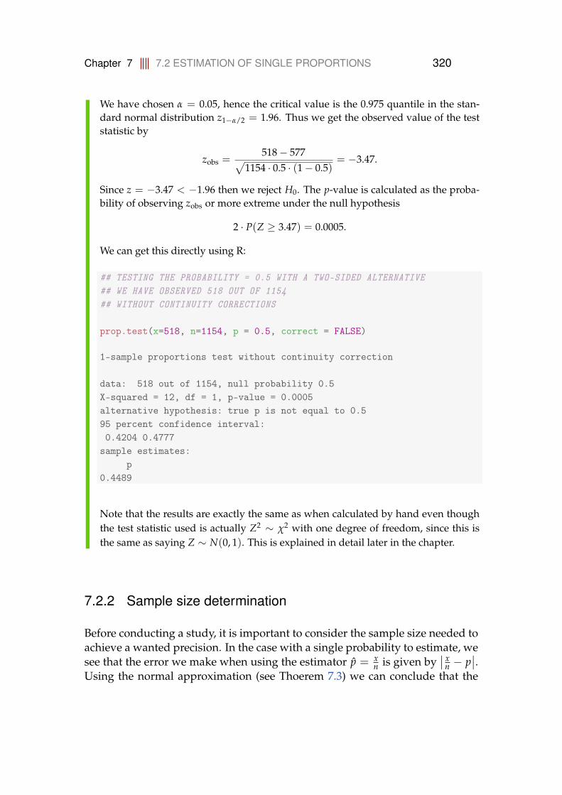
Chapter 7 7.2 ESTIMATION OF SINGLE PROPORTIONS 320
We have chosen α = 0.05, hence the critical value is the 0.975 quantile in the stan-dard normal distribution z1−α/2 = 1.96. Thus we get the observed value of the teststatistic by
zobs =518− 577√
1154 · 0.5 · (1− 0.5)= −3.47.
Since z = −3.47 < −1.96 then we reject H0. The p-value is calculated as the proba-bility of observing zobs or more extreme under the null hypothesis
2 · P(Z ≥ 3.47) = 0.0005.
We can get this directly using R:
## TESTING THE PROBABILITY = 0.5 WITH A TWO-SIDED ALTERNATIVE## WE HAVE OBSERVED 518 OUT OF 1154## WITHOUT CONTINUITY CORRECTIONS
prop.test(x=518, n=1154, p = 0.5, correct = FALSE)
1-sample proportions test without continuity correction
data: 518 out of 1154, null probability 0.5X-squared = 12, df = 1, p-value = 0.0005alternative hypothesis: true p is not equal to 0.595 percent confidence interval:0.4204 0.4777
sample estimates:p
0.4489
Note that the results are exactly the same as when calculated by hand even thoughthe test statistic used is actually Z2 ∼ χ2 with one degree of freedom, since this isthe same as saying Z ∼ N(0, 1). This is explained in detail later in the chapter.
7.2.2 Sample size determination
Before conducting a study, it is important to consider the sample size needed toachieve a wanted precision. In the case with a single probability to estimate, wesee that the error we make when using the estimator p = x
n is given by∣∣ x
n − p∣∣.
Using the normal approximation (see Thoerem 7.3) we can conclude that the
Chapter 7 7.3 COMPARING PROPORTIONS IN TWO POPULATIONS 321
error will be bounded by
∣∣∣ xn− p
∣∣∣ < z1−α/2
√p(1− p)
n, (7-22)
with probability 1− α. Thus the Margin of Error (ME) of the estimate becomes
ME = z1−α/2
√p(1− p)
n. (7-23)
Similar to the method given for quantitative data in Method 3.62, we can useEquation (7-23) to determine the needed sample size in a single proportionssetup. Solving for n we get:
Method 7.13 Sample size formula for the CI of a proportion
Given some “guess” (scenario) of the size of the unknown p, and given somerequirement to the ME-value (required expected precision) the necessarysample size is then
n = p(1− p)(z1−α/2
ME
)2. (7-24)
If p is unknown, a worst case scenario with p = 1/2 is applied and necessarysample size is
n =14
(z1−α/2
ME
)2. (7-25)
The expression in Equation (7-25) for n when no information about p is availableis due to the fact that p(1− p) is largest for p = 1/2, so the required sample sizewill be largest when p = 1/2.
Method 7.13 can be used to calculate the sample size for a given choice of ME.
7.3 Comparing proportions in two populations
For categorical variables we sometimes want to compare the proportions in twopopulations (groups). Let p1 denote the proportion in group 1 and p2 the pro-portion in group 2. We will compare the groups by looking at the difference inproportions p1 − p2, which is estimated by p1 − p2.

Chapter 7 7.3 COMPARING PROPORTIONS IN TWO POPULATIONS 322
Example 7.14
In a study in the US (1975) the relation between intake of contraceptive pills (birthcontrol pills) and the risk of blood clot in the heart was investigated. The followingdata were collected from a participating hospital:
Contraceptive pill No pillBlood clot 23 35No blood clot 34 132Total 57 167
We have a binary outcome blood clot (yes or no) and two groups (pill or no pill). Asin Section 7.2 we find that the best estimates of the unknown probabilities are theobserved proportions
p1 ="Number of blood clots in the pill group"
"Number of women in the pill group"=
2357
= 0.4035, (7-26)
p2 ="Number of blood clots in the no pill group"
"Number of women in the no pill group"=
35167
= 0.2096. (7-27)
The difference in probabilities is estimated to be
p1 − p2 = 0.4035− 0.2096 = 0.1939. (7-28)
Thus the observed probability of getting a blood clot, was 0.1939 higher in the con-traceptive pill group than in the no pill group.
We have the estimate p1 − p2 of the difference in probabilities p1 − p2 and theuncertainty of this estimate can be calculated by:

Chapter 7 7.3 COMPARING PROPORTIONS IN TWO POPULATIONS 323
Method 7.15
An estimate of the standard error of the estimator p1 − p2 is
σp1− p2 =
√p1(1− p1)
n1+
p2(1− p2)
n2. (7-29)
The (1− α)100% confidence interval for the difference p1 − p2 is
( p1 − p2)± z1−α/2 · σp1− p2 . (7-30)
This confidence interval requires independent random samples for the twogroups and large enough sample sizes n1 and n2. A rule of thumb is thatni pi ≥ 10 and ni(1− pi) ≥ 10 for i = 1, 2, must be satisfied.
Remark 7.16
The standard error in Method 7.15 can be calculated by
V( p1 − p2) = V( p1) + V( p2) = σ2p1+ σ2
p2, (7-31)
σp1− p2 =√
V( p1 − p2) =√
σ2p1+ σ2
p2. (7-32)
Notice, that the standard errors are added (before the square root) such thatthe standard error of the difference is larger than the standard error for theobserved proportions alone. Therefore in practice the estimate of the differ-ence p1 − p2 will often be further from the true difference p1 − p2 than p1will be from p1 or p2 will be from p2.
Example 7.17
Returning to Example 7.14 where we found the estimated difference in probabilityto be
p1 − p2 = 0.4035− 0.2096 = 0.1939. (7-33)
The estimated standard error of the estimate is
σp1− p2 =
√0.4035(1− 0.4035)
57+
0.2096(1− 0.2096)167
= 0.0722. (7-34)
A 99% confidence interval for this difference is then
( p1 − p2)± z0.995 · σp1− p2 = 0.1939± 2.5758 · 0.0722 = [0.0079, 0.3799]. (7-35)
Chapter 7 7.3 COMPARING PROPORTIONS IN TWO POPULATIONS 324
Hence our best estimate of the difference is 0.19 and with very high confidence thetrue difference is between 0.008 and 0.38.
We find that 0 is not included in the confidence interval, so 0 is not a plausible valuefor the difference p1 − p2. The values in the confidence interval are all positive andtherefore we can conclude that (p1 − p2) > 0, that is p1 > p2, i.e. the probability ofblood clot is larger in the contraceptive pill group than in the no pill group.
We can also compare the two proportions p1 and p2 using a hypothesis test. Asin Method 7.11, there are four steps when we want to carry out the test. Thefirst step is to formulate the hypothesis and the alternative.
The null hypothesis is H0 : p1 = p2 and we will denote the common proportionp, and choose a two-sided alternative H1 : p1 6= p2.
In the second step we calculate a test statistic measuring how far p1 − p2 fallsfrom 0, which is the value of p1 − p2 under H0.
Under H0, we only have one proportion p (since p1 = p2 = p). The best estima-tor for this common proportion is the overall observed proportion
p =x1 + x2
n1 + n2. (7-36)
When the two sample sizes n1 and n2 are similar, this pooled estmate of theoverall proportion will be approximately half way between p1 and p2, but oth-erwise the pooled estimate will be closest to the estimate from the largest samplesize.
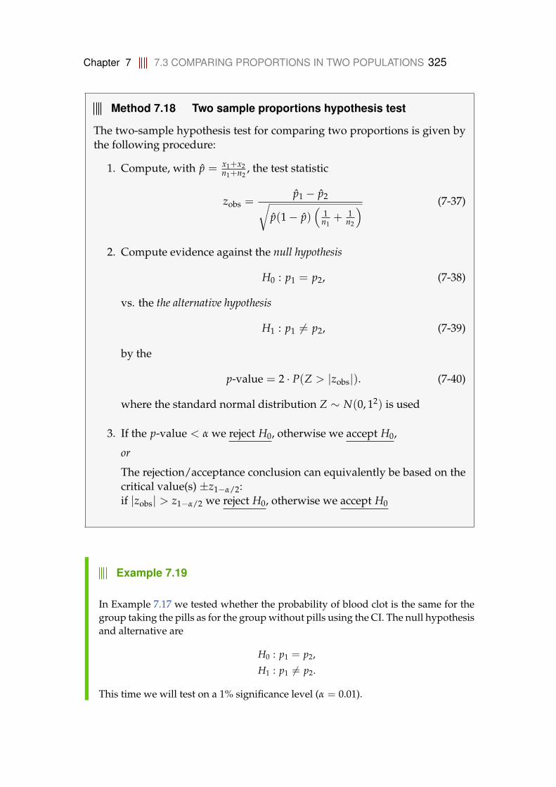
Chapter 7 7.3 COMPARING PROPORTIONS IN TWO POPULATIONS 325
Method 7.18 Two sample proportions hypothesis test
The two-sample hypothesis test for comparing two proportions is given bythe following procedure:
1. Compute, with p = x1+x2n1+n2
, the test statistic
zobs =p1 − p2√
p(1− p)(
1n1
+ 1n2
) (7-37)
2. Compute evidence against the null hypothesis
H0 : p1 = p2, (7-38)
vs. the the alternative hypothesis
H1 : p1 6= p2, (7-39)
by the
p-value = 2 · P(Z > |zobs|). (7-40)
where the standard normal distribution Z ∼ N(0, 12) is used
3. If the p-value < α we reject H0, otherwise we accept H0,
or
The rejection/acceptance conclusion can equivalently be based on thecritical value(s) ±z1−α/2:if |zobs| > z1−α/2 we reject H0, otherwise we accept H0
Example 7.19
In Example 7.17 we tested whether the probability of blood clot is the same for thegroup taking the pills as for the group without pills using the CI. The null hypothesisand alternative are
H0 : p1 = p2,
H1 : p1 6= p2.
This time we will test on a 1% significance level (α = 0.01).
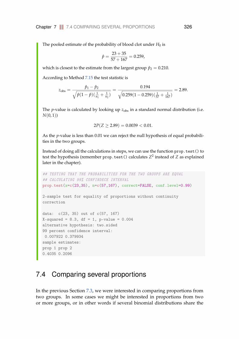
Chapter 7 7.4 COMPARING SEVERAL PROPORTIONS 326
The pooled estimate of the probability of blood clot under H0 is
p =23 + 35
57 + 167= 0.259,
which is closest to the estimate from the largest group p2 = 0.210.
According to Method 7.15 the test statistic is
zobs =p1 − p2√
p(1− p)( 1n1
+ 1n2)=
0.194√0.259(1− 0.259)( 1
57 +1
167 )= 2.89.
The p-value is calculated by looking up zobs in a standard normal distribution (i.e.N(0, 1))
2P(Z ≥ 2.89) = 0.0039 < 0.01.
As the p-value is less than 0.01 we can reject the null hypothesis of equal probabili-ties in the two groups.
Instead of doing all the calculations in steps, we can use the function prop.test() totest the hypothesis (remember prop.test() calculates Z2 instead of Z as explainedlater in the chapter).
## TESTING THAT THE PROBABILITIES FOR THE TWO GROUPS ARE EQUAL## CALCULATING 99% CONFINDECE INTERVALprop.test(x=c(23,35), n=c(57,167), correct=FALSE, conf.level=0.99)
2-sample test for equality of proportions without continuitycorrection
data: c(23, 35) out of c(57, 167)X-squared = 8.3, df = 1, p-value = 0.004alternative hypothesis: two.sided99 percent confidence interval:0.007922 0.379934
sample estimates:prop 1 prop 20.4035 0.2096
7.4 Comparing several proportions
In the previous Section 7.3, we were interested in comparing proportions fromtwo groups. In some cases we might be interested in proportions from twoor more groups, or in other words if several binomial distributions share the
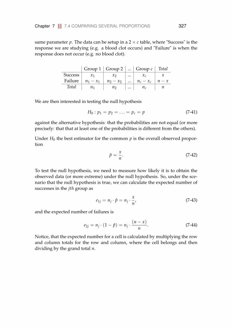
Chapter 7 7.4 COMPARING SEVERAL PROPORTIONS 327
same parameter p. The data can be setup in a 2× c table, where "Success" is theresponse we are studying (e.g. a blood clot occurs) and "Failure" is when theresponse does not occur (e.g. no blood clot).
Group 1 Group 2 ... Group c TotalSuccess x1 x2 ... xc xFailure n1 − x1 n2 − x2 ... nc − xc n− x
Total n1 n2 ... nc n
We are then interested in testing the null hypothesis
H0 : p1 = p2 = . . . = pc = p (7-41)
against the alternative hypothesis: that the probabilities are not equal (or moreprecisely: that that at least one of the probabilities is different from the others).
Under H0 the best estimator for the common p is the overall observed propor-tion
p =xn
. (7-42)
To test the null hypothesis, we need to measure how likely it is to obtain theobserved data (or more extreme) under the null hypothesis. So, under the sce-nario that the null hypothesis is true, we can calculate the expected number ofsuccesses in the jth group as
e1j = nj · p = nj ·xn
, (7-43)
and the expected number of failures is
e2j = nj · (1− p) = nj ·(n− x)
n. (7-44)
Notice, that the expected number for a cell is calculated by multiplying the rowand column totals for the row and column, where the cell belongs and thendividing by the grand total n.
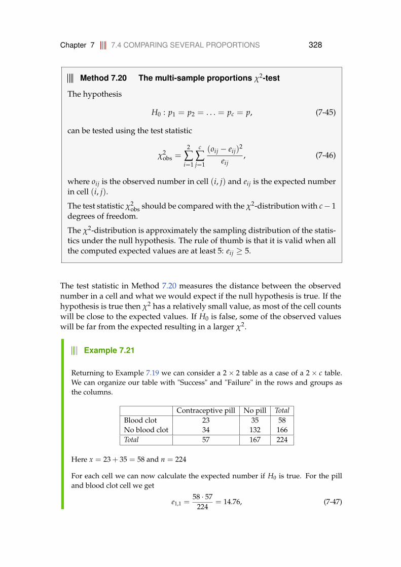
Chapter 7 7.4 COMPARING SEVERAL PROPORTIONS 328
Method 7.20 The multi-sample proportions χ2-test
The hypothesis
H0 : p1 = p2 = . . . = pc = p, (7-45)
can be tested using the test statistic
χ2obs =
2
∑i=1
c
∑j=1
(oij − eij)2
eij, (7-46)
where oij is the observed number in cell (i, j) and eij is the expected numberin cell (i, j).
The test statistic χ2obs should be compared with the χ2-distribution with c− 1
degrees of freedom.
The χ2-distribution is approximately the sampling distribution of the statis-tics under the null hypothesis. The rule of thumb is that it is valid when allthe computed expected values are at least 5: eij ≥ 5.
The test statistic in Method 7.20 measures the distance between the observednumber in a cell and what we would expect if the null hypothesis is true. If thehypothesis is true then χ2 has a relatively small value, as most of the cell countswill be close to the expected values. If H0 is false, some of the observed valueswill be far from the expected resulting in a larger χ2.
Example 7.21
Returning to Example 7.19 we can consider a 2× 2 table as a case of a 2× c table.We can organize our table with "Success" and "Failure" in the rows and groups asthe columns.
Contraceptive pill No pill TotalBlood clot 23 35 58No blood clot 34 132 166Total 57 167 224
Here x = 23 + 35 = 58 and n = 224
For each cell we can now calculate the expected number if H0 is true. For the pilland blood clot cell we get
e1,1 =58 · 57
224= 14.76, (7-47)
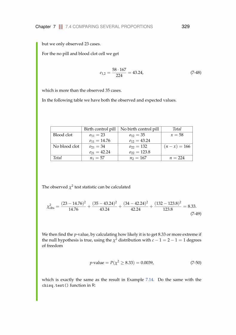
Chapter 7 7.4 COMPARING SEVERAL PROPORTIONS 329
but we only observed 23 cases.
For the no pill and blood clot cell we get
e1,2 =58 · 167
224= 43.24, (7-48)
which is more than the observed 35 cases.
In the following table we have both the observed and expected values.
Birth control pill No birth control pill TotalBlood clot o11 = 23 o12 = 35 x = 58
e11 = 14.76 e12 = 43.24No blood clot o21 = 34 o22 = 132 (n− x) = 166
e21 = 42.24 o22 = 123.8Total n1 = 57 n2 = 167 n = 224
The observed χ2 test statistic can be calculated
χ2obs =
(23− 14.76)2
14.76+
(35− 43.24)2
43.24+
(34− 42.24)2
42.24+
(132− 123.8)2
123.8= 8.33.
(7-49)
We then find the p-value, by calculating how likely it is to get 8.33 or more extreme ifthe null hypothesis is true, using the χ2 distribution with c− 1 = 2− 1 = 1 degreesof freedom
p-value = P(χ2 ≥ 8.33) = 0.0039, (7-50)
which is exactly the same as the result in Example 7.14. Do the same with thechisq.test() function in R:
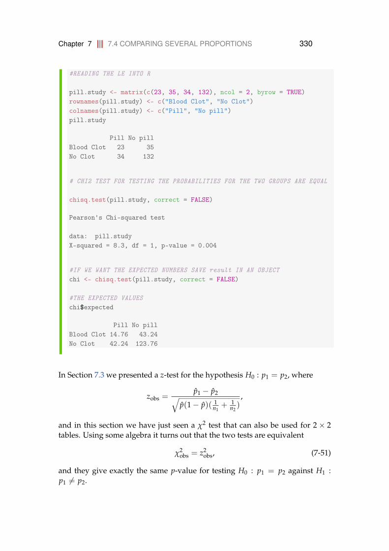
Chapter 7 7.4 COMPARING SEVERAL PROPORTIONS 330
#READING THE LE INTO R
pill.study <- matrix(c(23, 35, 34, 132), ncol = 2, byrow = TRUE)rownames(pill.study) <- c("Blood Clot", "No Clot")colnames(pill.study) <- c("Pill", "No pill")pill.study
Pill No pillBlood Clot 23 35No Clot 34 132
# CHI2 TEST FOR TESTING THE PROBABILITIES FOR THE TWO GROUPS ARE EQUAL
chisq.test(pill.study, correct = FALSE)
Pearson's Chi-squared test
data: pill.studyX-squared = 8.3, df = 1, p-value = 0.004
#IF WE WANT THE EXPECTED NUMBERS SAVE result IN AN OBJECTchi <- chisq.test(pill.study, correct = FALSE)
#THE EXPECTED VALUESchi$expected
Pill No pillBlood Clot 14.76 43.24No Clot 42.24 123.76
In Section 7.3 we presented a z-test for the hypothesis H0 : p1 = p2, where
zobs =p1 − p2√
p(1− p)( 1n1
+ 1n2)
,
and in this section we have just seen a χ2 test that can also be used for 2× 2tables. Using some algebra it turns out that the two tests are equivalent
χ2obs = z2
obs, (7-51)
and they give exactly the same p-value for testing H0 : p1 = p2 against H1 :p1 6= p2.
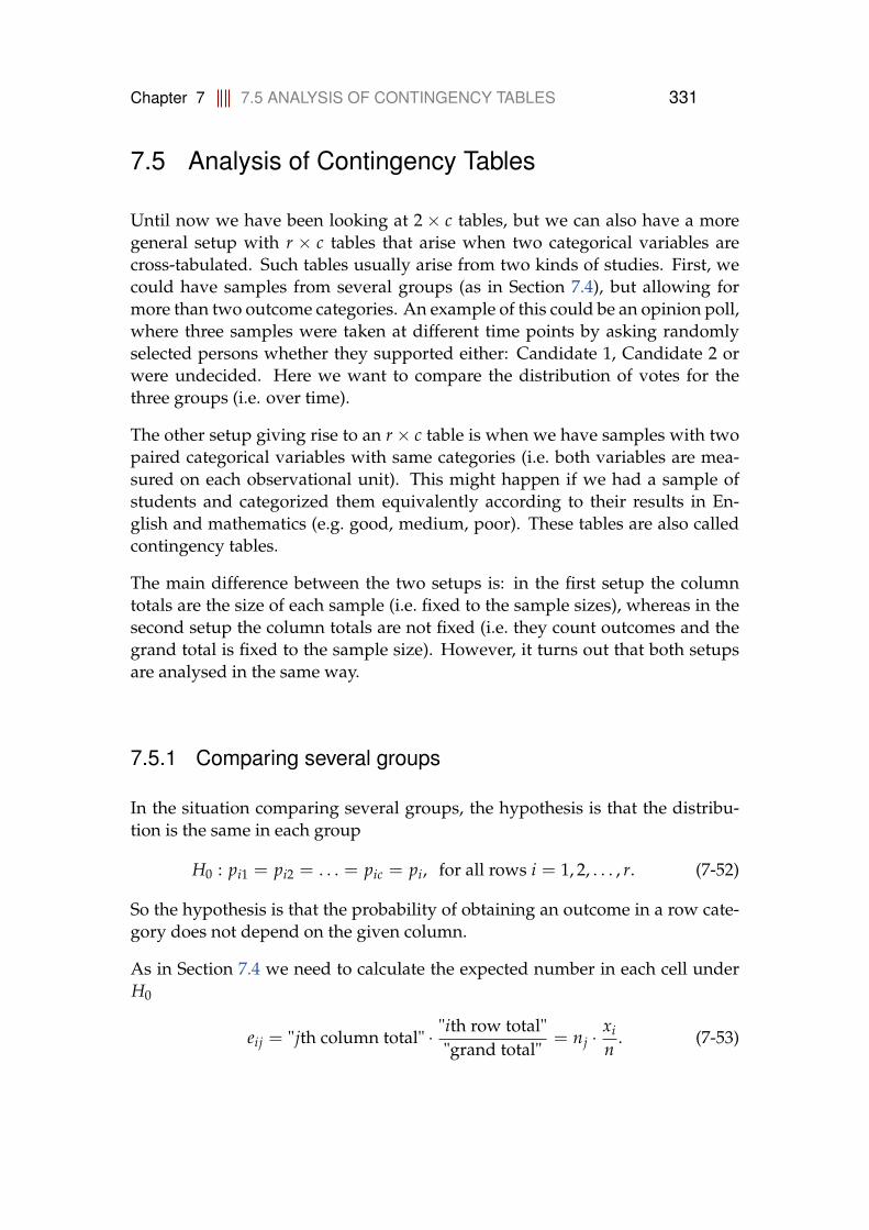
Chapter 7 7.5 ANALYSIS OF CONTINGENCY TABLES 331
7.5 Analysis of Contingency Tables
Until now we have been looking at 2× c tables, but we can also have a moregeneral setup with r × c tables that arise when two categorical variables arecross-tabulated. Such tables usually arise from two kinds of studies. First, wecould have samples from several groups (as in Section 7.4), but allowing formore than two outcome categories. An example of this could be an opinion poll,where three samples were taken at different time points by asking randomlyselected persons whether they supported either: Candidate 1, Candidate 2 orwere undecided. Here we want to compare the distribution of votes for thethree groups (i.e. over time).
The other setup giving rise to an r× c table is when we have samples with twopaired categorical variables with same categories (i.e. both variables are mea-sured on each observational unit). This might happen if we had a sample ofstudents and categorized them equivalently according to their results in En-glish and mathematics (e.g. good, medium, poor). These tables are also calledcontingency tables.
The main difference between the two setups is: in the first setup the columntotals are the size of each sample (i.e. fixed to the sample sizes), whereas in thesecond setup the column totals are not fixed (i.e. they count outcomes and thegrand total is fixed to the sample size). However, it turns out that both setupsare analysed in the same way.
7.5.1 Comparing several groups
In the situation comparing several groups, the hypothesis is that the distribu-tion is the same in each group
H0 : pi1 = pi2 = . . . = pic = pi, for all rows i = 1, 2, . . . , r. (7-52)
So the hypothesis is that the probability of obtaining an outcome in a row cate-gory does not depend on the given column.
As in Section 7.4 we need to calculate the expected number in each cell underH0
eij = "jth column total" · "ith row total""grand total"
= nj ·xi
n. (7-53)
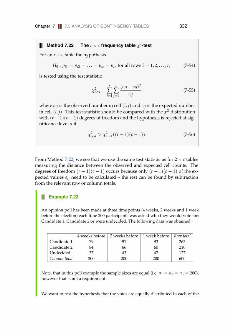
Chapter 7 7.5 ANALYSIS OF CONTINGENCY TABLES 332
Method 7.22 The r× c frequency table χ2-test
For an r× c table the hypothesis
H0 : pi1 = pi2 = . . . = pic = pi, for all rows i = 1, 2, . . . , r, (7-54)
is tested using the test statistic
χ2obs =
r
∑i=1
c
∑j=1
(oij − eij)2
eij. (7-55)
where oij is the observed number in cell (i, j) and eij is the expected numberin cell (i, j). This test statistic should be compared with the χ2-distributionwith (r− 1)(c− 1) degrees of freedom and the hypothesis is rejected at sig-nificance level α if
χ2obs > χ2
1−α
((r− 1)(c− 1)
). (7-56)
From Method 7.22, we see that we use the same test statistic as for 2× c tablesmeasuring the distance between the observed and expected cell counts. Thedegrees of freedom (r− 1)(c− 1) occurs because only (r− 1)(c− 1) of the ex-pected values eij need to be calculated – the rest can be found by subtractionfrom the relevant row or column totals.
Example 7.23
An opinion poll has been made at three time points (4 weeks, 2 weeks and 1 weekbefore the election) each time 200 participants was asked who they would vote for:Candidate 1, Candidate 2 or were undecided. The following data was obtained:
4 weeks before 2 weeks before 1 week before Row totalCandidate 1 79 91 93 263Candidate 2 84 66 60 210Undecided 37 43 47 127Column total 200 200 200 600
Note, that in this poll example the sample sizes are equal (i.e. n1 = n2 = n3 = 200),however that is not a requirement.
We want to test the hypothesis that the votes are equally distributed in each of the
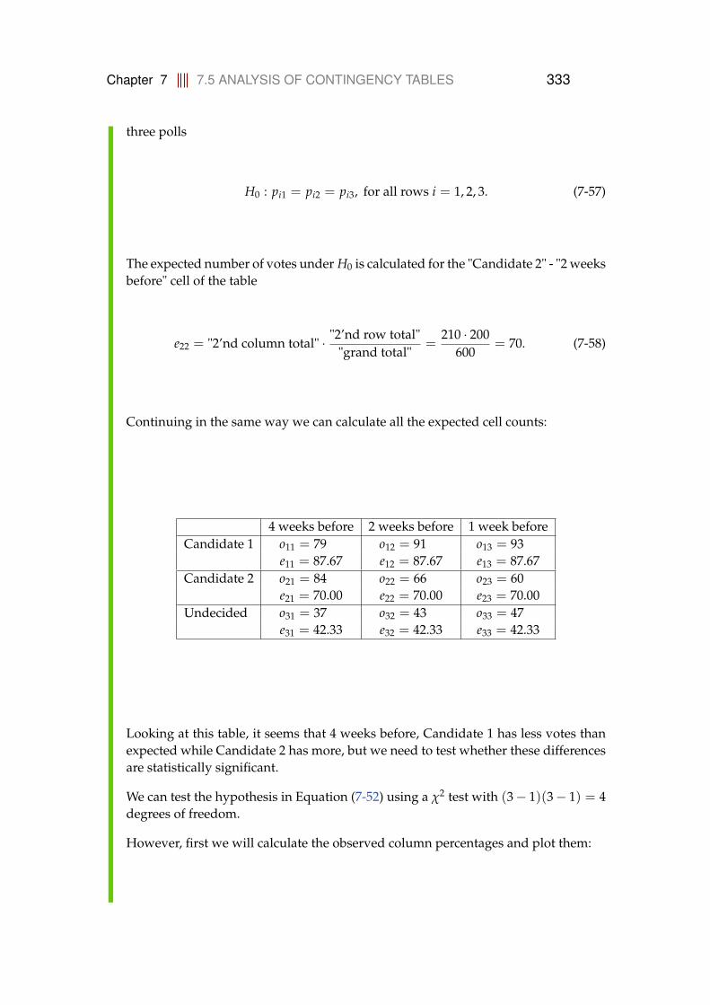
Chapter 7 7.5 ANALYSIS OF CONTINGENCY TABLES 333
three polls
H0 : pi1 = pi2 = pi3, for all rows i = 1, 2, 3. (7-57)
The expected number of votes under H0 is calculated for the "Candidate 2" - "2 weeksbefore" cell of the table
e22 = "2’nd column total" · "2’nd row total""grand total"
=210 · 200
600= 70. (7-58)
Continuing in the same way we can calculate all the expected cell counts:
4 weeks before 2 weeks before 1 week beforeCandidate 1 o11 = 79 o12 = 91 o13 = 93
e11 = 87.67 e12 = 87.67 e13 = 87.67Candidate 2 o21 = 84 o22 = 66 o23 = 60
e21 = 70.00 e22 = 70.00 e23 = 70.00Undecided o31 = 37 o32 = 43 o33 = 47
e31 = 42.33 e32 = 42.33 e33 = 42.33
Looking at this table, it seems that 4 weeks before, Candidate 1 has less votes thanexpected while Candidate 2 has more, but we need to test whether these differencesare statistically significant.
We can test the hypothesis in Equation (7-52) using a χ2 test with (3− 1)(3− 1) = 4degrees of freedom.
However, first we will calculate the observed column percentages and plot them:
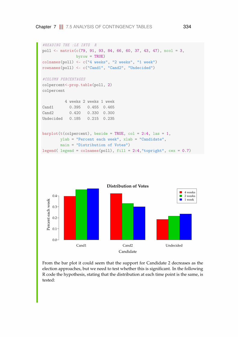
Chapter 7 7.5 ANALYSIS OF CONTINGENCY TABLES 334
#READING THE :LE INTO Rpoll <- matrix(c(79, 91, 93, 84, 66, 60, 37, 43, 47), ncol = 3,
byrow = TRUE)colnames(poll) <- c("4 weeks", "2 weeks", "1 week")rownames(poll) <- c("Cand1", "Cand2", "Undecided")
#COLUMN PERCENTAGEScolpercent<-prop.table(poll, 2)colpercent
4 weeks 2 weeks 1 weekCand1 0.395 0.455 0.465Cand2 0.420 0.330 0.300Undecided 0.185 0.215 0.235
barplot(t(colpercent), beside = TRUE, col = 2:4, las = 1,ylab = "Percent each week", xlab = "Candidate",main = "Distribution of Votes")
legend( legend = colnames(poll), fill = 2:4,"topright", cex = 0.7)
Cand1 Cand2 Undecided
Distribution of Votes
Candidate
Perc
ente
ach
wee
k
0.0
0.1
0.2
0.3
0.44 weeks2 weeks1 week
From the bar plot it could seem that the support for Candidate 2 decreases as theelection approaches, but we need to test whether this is significant. In the followingR code the hypothesis, stating that the distribution at each time point is the same, istested:
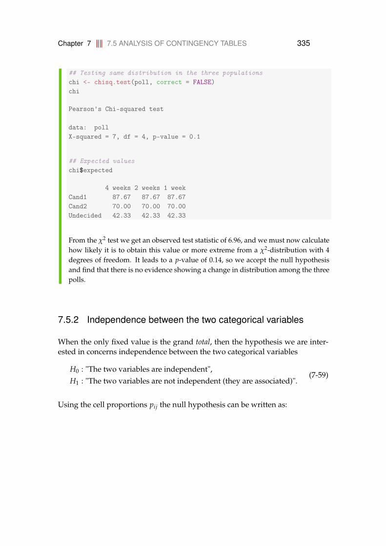
Chapter 7 7.5 ANALYSIS OF CONTINGENCY TABLES 335
## Testing same distribution in the three populationschi <- chisq.test(poll, correct = FALSE)chi
Pearson's Chi-squared test
data: pollX-squared = 7, df = 4, p-value = 0.1
## Expected valueschi$expected
4 weeks 2 weeks 1 weekCand1 87.67 87.67 87.67Cand2 70.00 70.00 70.00Undecided 42.33 42.33 42.33
From the χ2 test we get an observed test statistic of 6.96, and we must now calculatehow likely it is to obtain this value or more extreme from a χ2-distribution with 4degrees of freedom. It leads to a p-value of 0.14, so we accept the null hypothesisand find that there is no evidence showing a change in distribution among the threepolls.
7.5.2 Independence between the two categorical variables
When the only fixed value is the grand total, then the hypothesis we are inter-ested in concerns independence between the two categorical variables
H0 : "The two variables are independent",H1 : "The two variables are not independent (they are associated)".
(7-59)
Using the cell proportions pij the null hypothesis can be written as:
Chapter 7 7.5 ANALYSIS OF CONTINGENCY TABLES 336
Theorem 7.24
To test if two categorical variables are independent the null hypothesis
H0 : pij = pi.p.j for all i, j, (7-60)
where pi. = ∑cj=1 pij is the proportion of row i and p.j = ∑r
i=1 pij is theproportion of column j, is tested.
The p-value for the observed result under this null hypothesis is calculatedusing the χ2 test statistic from Method 7.22.
Example 7.25
A group of 400 students have had an English test and a mathematics test. The resultsof each test a categorized as either bad, average or good.
English MathematicsBad Average Good Row total
Bad 23 60 29 112Average 28 79 60 167Good 9 49 63 121Column total 60 188 152 400
We want to test the hypothesis of independence between results in English andmathematics. First we read the data into R and calculate proportions and totals:
## READING THE LE INTO Rresults <- matrix(c(23, 60, 29, 28, 79, 60, 9, 49, 63), ncol = 3,
byrow = TRUE)colnames(results) <- c("MathBad", "MathAve", "MathGood")rownames(results) <- c("EngBad", "EngAve", "EngGood")

Chapter 7 7.5 ANALYSIS OF CONTINGENCY TABLES 337
#PERCENTAGESprop.table(results)
MathBad MathAve MathGoodEngBad 0.0575 0.1500 0.0725EngAve 0.0700 0.1975 0.1500EngGood 0.0225 0.1225 0.1575
#ROW TOTALSmargin.table(results, 1)
EngBad EngAve EngGood112 167 121
#COLUMN TOTALSmargin.table(results, 2)
MathBad MathAve MathGood60 188 152
We want to calculate the expected cell count if H0 is true. Consider the events "goodEnglish result" and "good mathematics result" corresponding to cell (3, 3). Underthe hypothesis of independence, we have
p33 = P("Good English and Good Maths") = P("Good English") · P("Good Maths")(7-61)
From the calculated row and column totals, we would estimate
p33 =
(121400
)·(
152400
), (7-62)
and out of 400 students we would expect
e33 = 400 · p33 = 400 ·(
121400
)·(
152400
)= 121 · 152
400= 45.98. (7-63)
The method of calculating the expected cell counts is exactly as before. For the“Good English and Good Mathematics” cell the expected value is less than the ob-served 63. Continuing in this way, we can calculate all the expected cell counts:
English MathematicsBad Average Good
Bad o11 = 23 o12 = 60 o13 = 29e11 = 16.80 e12 = 52.64 e13 = 42.56
Average o21 = 28 o22 = 79 o23 = 60e21 = 25.05 e22 = 78.49 e23 = 63.46
Good o31 = 9 o32 = 49 o33 = 63e31 = 18.15 e32 = 56.87 e33 = 45.98
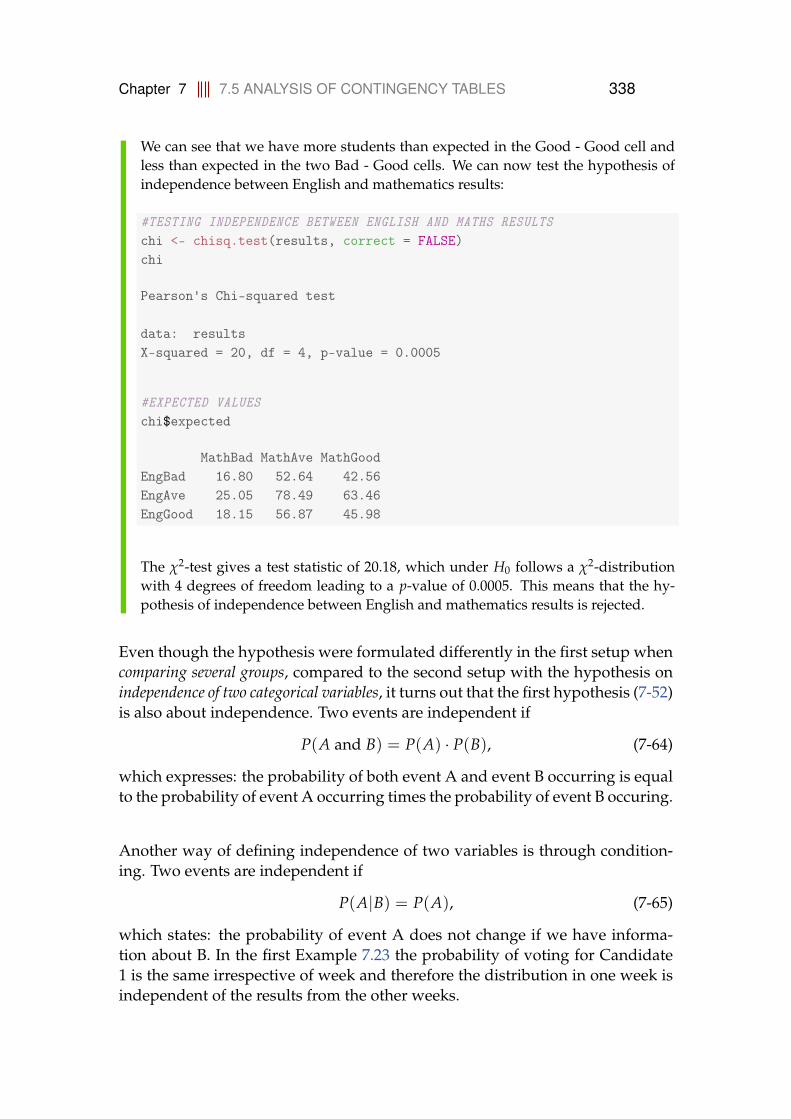
Chapter 7 7.5 ANALYSIS OF CONTINGENCY TABLES 338
We can see that we have more students than expected in the Good - Good cell andless than expected in the two Bad - Good cells. We can now test the hypothesis ofindependence between English and mathematics results:
#TESTING INDEPENDENCE BETWEEN ENGLISH AND MATHS RESULTSchi <- chisq.test(results, correct = FALSE)chi
Pearson's Chi-squared test
data: resultsX-squared = 20, df = 4, p-value = 0.0005
#EXPECTED VALUESchi$expected
MathBad MathAve MathGoodEngBad 16.80 52.64 42.56EngAve 25.05 78.49 63.46EngGood 18.15 56.87 45.98
The χ2-test gives a test statistic of 20.18, which under H0 follows a χ2-distributionwith 4 degrees of freedom leading to a p-value of 0.0005. This means that the hy-pothesis of independence between English and mathematics results is rejected.
Even though the hypothesis were formulated differently in the first setup whencomparing several groups, compared to the second setup with the hypothesis onindependence of two categorical variables, it turns out that the first hypothesis (7-52)is also about independence. Two events are independent if
P(A and B) = P(A) · P(B), (7-64)
which expresses: the probability of both event A and event B occurring is equalto the probability of event A occurring times the probability of event B occuring.
Another way of defining independence of two variables is through condition-ing. Two events are independent if
P(A|B) = P(A), (7-65)
which states: the probability of event A does not change if we have informa-tion about B. In the first Example 7.23 the probability of voting for Candidate1 is the same irrespective of week and therefore the distribution in one week isindependent of the results from the other weeks.
Chapter 7 7.6 EXERCISES 339
7.6 Exercises
Exercise 7.1 Passing proportions
To compare the level of 2 different courses at a university the following gradesdistributions (given as number of pupils who achieved the grades) were regis-tered:
Course 1 Course 2 Row totalGrade 12 20 14 34Grade 10 14 14 28Grade 7 16 27 43Grade 4 20 22 42Grade 2 12 27 39Grade 0 16 17 33Grade -3 10 22 32Column total 108 143 251
The passing proportions for the two courses, p1 and p2 should be compared. Asthe grades -3 and 0 means not passed, we get the following table of the numberof students:
Course 1 Course 2 Row totalPassed 82 104 186Not passed 26 39 65Column total 108 143 251
a) Compute a 95% confidence interval for the difference between the twopassing proportions.
b) What is the critical values for the χ2-test of the hypothesis H0 : p1 = p2with significance level α = 0.01?
c) If the passing proportion for a course given repeatedly is assumed to be0.80 on average, and there are 250 students who are taking the exam eachtime, what is the expected value, µ and standard deviation, σ, for the num-ber of students who do not pass the exam for a randomly selected course?
Chapter 7 7.6 EXERCISES 340
Exercise 7.2 Outdoor lighting
A company that sells outdoor lighting, gets a lamp produced in 3 material vari-ations: in copper, with painted surface and with stainless steel. The lamps aresold partly in Denmark and partly for export. For 250 lamps the distribution ofsales between the three variants and Denmark/export are depicted. The data isshown in the following table:
CountryDanmark Export
Copper variant 7.2% 6.4%Painted variant 28.0% 34.8%Stainless steel variant 8.8% 14.8%
a) Is there a significant difference between the proportion exported and theproportion sold in Denmark (with α = 0.05)?
b) The relevant critical value to use for testing whether there is a significantdifference in how the sold variants are distributed in Denmark and forexport is (with α = 0.05)?
Exercise 7.3 Local elections
At the local elections in Denmark in November 2013 the Social Democrats (A)had p = 29.5% of the votes at the country level. From an early so-called exitpoll it was estimated that they would only get 22.7% of the votes. Suppose theexit poll was based on 740 people out of which then 168 people reported havingvoted for A.
a) At the time of the exit poll the p was of course not known. If the followinghypothesis was tested based on the exit poll
H0 : p = 0.295H1 : p 6= 0.295,
what test statistic and conclusion would then be obtained with α = 0.001?
Chapter 7 7.6 EXERCISES 341
b) Calculate a 95%-confidence interval for p based on the exit poll.
c) Based on a scenario that the proportion voting for particular party is around30%, how large an exit poll should be taken to achieve a 99% confidenceinterval having a width of 0.01 in average for this proportion?
Exercise 7.4 Sugar quality
A wholesaler needs to find a supplier that delivers sugar in 1 kg bags. From twopotential suppliers 50 bags of sugar are received from each. A bag is describedas ’defective’ if the weight of the filled bag is less than 990 grams. The receivedbags were all control weighed and 6 defective from supplier A and 12 defectivefrom supplier B were found.
a) If the following hypothesis is tested
H0 : pA = pB,H1 : pA 6= pB.
What is the p-value?
b) A supplier has delivered 200 bags, of which 36 were defective. A 99%confidence interval for p the proportion of defective bags for this supplieris:
c) Based on the scenario, that the proportion of defective bags for a new sup-plier is about 20%, a new study was planned with the aim of obtaining anaverage width, B, of a 95% confidence interval. The Analysis Departmentachieved the result that one should examine 1537 bags, but had forgottento specify which value for the width B, they had used. What was the valueused for B?
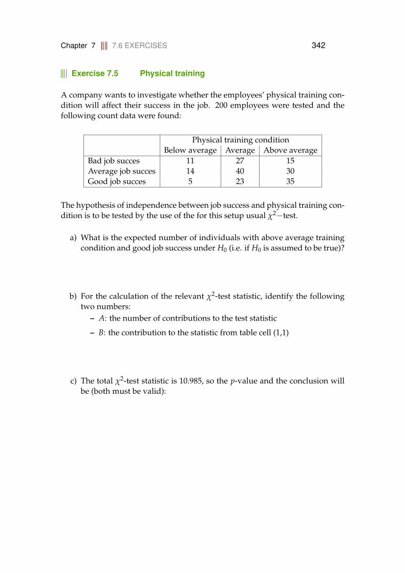
Chapter 7 7.6 EXERCISES 342
Exercise 7.5 Physical training
A company wants to investigate whether the employees’ physical training con-dition will affect their success in the job. 200 employees were tested and thefollowing count data were found:
Physical training conditionBelow average Average Above average
Bad job succes 11 27 15Average job succes 14 40 30Good job succes 5 23 35
The hypothesis of independence between job success and physical training con-dition is to be tested by the use of the for this setup usual χ2−test.
a) What is the expected number of individuals with above average trainingcondition and good job success under H0 (i.e. if H0 is assumed to be true)?
b) For the calculation of the relevant χ2-test statistic, identify the followingtwo numbers:
– A: the number of contributions to the test statistic
– B: the contribution to the statistic from table cell (1,1)
c) The total χ2-test statistic is 10.985, so the p-value and the conclusion willbe (both must be valid):
Chapter 8 343
Chapter 8
Comparing means of multiple groups- ANOVA
8.1 Introduction
In Chapter 3 the test of difference in mean of two groups was introduced
H0 : µ1 − µ2 = δ0. (8-1)
Often we are interested in testing if the mean of the two groups are different(H0 : µ1 = µ2), against the alternative (µ1 6= µ2). Often we will face a situ-ation where we have data in multiple (more than two) groups leading to thenatural extension of the two-sample situation to a multi-sample situation. Thehypothesis of k groups having the same means can then be expressed as:
H0 : µ1 = µ2 = · · · = µk. (8-2)
Or in words we have k groups (often refered to as treatments) and we want totest if they all have the same mean against the alternative that at least one groupis different from the other groups. Note, that the hypothesis is not expressingany particular values for the means, but just that they are all the same.
The purpose of the data analysis in such a multigroup situation can be ex-pressed as a two-fold purpose:
1. Answer the question: are the group means (significantly) different (hy-pothesis test)?
2. Tell the story about (or “quantify”) the groups and their potential differ-ences (estimates and confidence intervals)
Chapter 8 8.2 ONE-WAY ANOVA 344
The statistical analysis used for such an analysis is called one-way Analysisof Variance (ANOVA). Though there is an initial contradiction in the name, asANOVA is used to compare the means of populations and not their variances,the name should not be met with confusion. An ANOVA expresses how dif-ferent the means of k populations are by measuring how much of the variancein data is explained by grouping the observations (in other words: the varianceexplained by fitting a model with a mean for each population). If enough of thevariation is explained, then a significant difference in population means can beconcluded.
The one-way ANOVA is the natural multi-sample extension of the indepen-dent two-sample setup covered in Chapter 3. We will also present a naturalmulti-sample extension of the two paired-sample situation from Chapter 3. Thisgeneralization, where the k samples are somehow dependent, e.g. if the sameindividuals are used in each of the groups, is called two-way ANOVA.
8.2 One-way ANOVA
8.2.1 Data structure and model
As mentioned above we assume that we have data from k groups, also assumeni repetitions in group (i), this imply that we can order data in a table like:
Tr1 y11 . . . y1,n1...
... . . .Trk yk,1 . . . yk,nk
The total number of observations is n = ∑ki=1 ni, note that there does not have
to be the same number of observations within each group (treatment).
As for the two-sample case in Chapter 3 there are some standard assumptionsthat are usually made in order for the methods to come to be 100% valid. Inthe case of one-way ANOVA, these assumptions are expressed by formulatinga “model” much like how regression models in Chapters 5 and 6 are expressed
Yij = µi + εij, εij ∼ N(0, σ2). (8-3)
The model is expressing that the observations come from a normal distributionwithin each group, that each group (i) has a specific mean, and that the varianceis the same (σ2) for all groups. Further, we see explicitly that we have a numberof observations (ni) within each group (j = 1, . . . , ni).
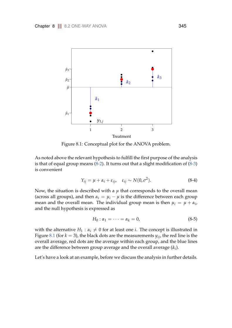
Chapter 8 8.2 ONE-WAY ANOVA 345
Treatment
1 2 3
µ1
µ
µ2
µ3
α1
α2
α3
y1,j
Figure 8.1: Conceptual plot for the ANOVA problem.
As noted above the relevant hypothesis to fulfill the first purpose of the analysisis that of equal group means (8-2). It turns out that a slight modification of (8-3)is convenient
Yij = µ + αi + εij, εij ∼ N(0, σ2). (8-4)
Now, the situation is described with a µ that corresponds to the overall mean(across all groups), and then αi = µi − µ is the difference between each groupmean and the overall mean. The individual group mean is then µi = µ + αi,and the null hypothesis is expressed as
H0 : α1 = · · · = αk = 0, (8-5)
with the alternative H1 : αi 6= 0 for at least one i. The concept is illustrated inFigure 8.1 (for k = 3), the black dots are the measurements yij, the red line is theoverall average, red dots are the average within each group, and the blue linesare the difference between group average and the overall average (αi).
Let’s have a look at an example, before we discuss the analysis in further details.
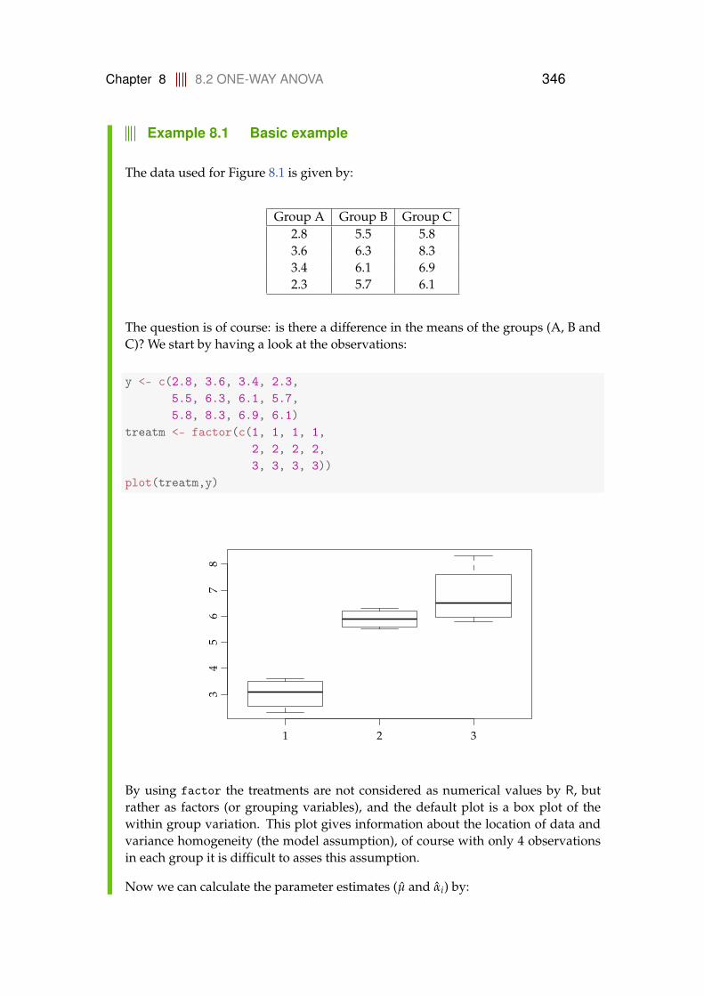
Chapter 8 8.2 ONE-WAY ANOVA 346
Example 8.1 Basic example
The data used for Figure 8.1 is given by:
Group A Group B Group C2.8 5.5 5.83.6 6.3 8.33.4 6.1 6.92.3 5.7 6.1
The question is of course: is there a difference in the means of the groups (A, B andC)? We start by having a look at the observations:
y <- c(2.8, 3.6, 3.4, 2.3,5.5, 6.3, 6.1, 5.7,5.8, 8.3, 6.9, 6.1)
treatm <- factor(c(1, 1, 1, 1,2, 2, 2, 2,3, 3, 3, 3))
plot(treatm,y)
1 2 3
34
56
78
By using factor the treatments are not considered as numerical values by R, butrather as factors (or grouping variables), and the default plot is a box plot of thewithin group variation. This plot gives information about the location of data andvariance homogeneity (the model assumption), of course with only 4 observationsin each group it is difficult to asses this assumption.
Now we can calculate the parameter estimates (µ and αi) by:

Chapter 8 8.2 ONE-WAY ANOVA 347
mu <- mean(y)muis <- tapply(y, treatm, mean)alpha <- muis - mumu
[1] 5.233
muis
1 2 33.025 5.900 6.775
alpha
1 2 3-2.2083 0.6667 1.5417
So our estimate of the overall mean is µ = 5.23, and the group levels (offsets fromthe overall sample mean) are α1 = −2.21, α2 = 0.67 and α3 = 1.54. The question weneed to answer is: how likely is it that the observed differences in group means arerandom variation? If this is very unlikely, then it can be concluded that at least oneof them is significantly different from zero.
The shown use of the tapply function is a convenient way of finding the mean of yfor each level of the factor treatm. By the way if the mean is substituted by any otherR-function, e.g. the variance, we could similarly find the sample variance withineach group (we will have a closer look at these later):
tapply(y, treatm, var)
1 2 30.3492 0.1333 1.2492
8.2.2 Decomposition of variability, the ANOVA table
A characteristic of ANOVA in general and one-way ANOVA specifically is thefact that the overall variability (measured by the total variation) decomposesinto interpretable components – it is these components which are used for hy-pothesis testing and more. For the one-way ANOVA presented in this sectionthe total variation, that is, the variation calculated across all the data completely
Chapter 8 8.2 ONE-WAY ANOVA 348
ignoring the fact that the data falls in different groups, can be decomposed intotwo components: a component expressing the group differences and a compo-nent expressing the (average) variation within the groups:
Theorem 8.2 Variability decomposition
The total sum of squares (SST) can be decomposed into sum of squarederrors (SSE) and treatment sum of squares (SS(Tr))
k
∑i=1
ni
∑j=1
(yij − y)2
︸ ︷︷ ︸SST
=k
∑i=1
ni
∑j=1
(yij − yi)2
︸ ︷︷ ︸SSE
+k
∑i=1
ni(yi − y)2
︸ ︷︷ ︸SS(Tr)
, (8-6)
where
y =1n
k
∑j=1
ni
∑j=1
yij, yi =1ni
ni
∑j=1
yij. (8-7)
Expressed in short form
SST = SS(Tr) + SSE. (8-8)
Before we turn to the proof of the theorem, we will briefly discuss some in-terpretations and implications of this. First we look at each of the three termsseparately.
The SST expresses the total variation. Let us compare with Equation (1-6) theformula for sample variance
s2 =1
n− 1
n
∑i=1
(xi − x)2. (8-9)
We can see that if the sample variance formula was applied to all the yijs in thatsetting (by simply joining them as a single sample), we see that with dividingwith n − 1 we have SST. The double sum of the SST definition is simply theformal way to express a summation of all double indexed observations yij. Orsimilarly expressed, if we call the (one-sample) variance of all the yijs, s2
y:
SST = (n− 1) · s2y. (8-10)
The group mean differences are quantified by the SS(Tr) component, as is ba-sically directly seen from the definition, where the overall mean is subtracted

Chapter 8 8.2 ONE-WAY ANOVA 349
from each group mean. As discussed above this could then alternatively beexpressed by the name of these deviations αi:
SS(Tr) =k
∑i=1
ni(yi − y)2 =k
∑i=1
niα2i , (8-11)
so SS(Tr) is the sum of squared αi’s multiplied by the number of observationsin group ni.
Remark 8.3
SS(Tr) is also the key expression to get the idea of why we call the wholething “analysis of variance”: if we, for a second, assume that we have thesame number of observations in each group: n1 = · · · = nk, and let us callthis common number m. Then we can express SS(Tr) directly in terms of thevariance of the k means
SS(Tr) = (k− 1) ·m · s2means, (8-12)
where
s2means =
1k− 1
k
∑i=1
(yi − y)2. (8-13)
Let us emphasize that the formulas of this remark is not thought to be for-mulas that we use for practical purposes, but they are expressed to showexplicitly that “SS(Tr) quantifies the group differences by variation”.
Finally, SSE expresses the average variability within each group, as each in-dividual observation yij is compared with the mean in the group to which itbelongs. In Figure 8.1 these are the differences between each of the black dotswith the relevant read dot. Again we can link the formula given above to basicuses of the sample variance formula:
Chapter 8 8.2 ONE-WAY ANOVA 350
Theorem 8.4 Within group variability
The sum of squared errors SSE divided by n − k, also called the residualmean square MSE = SSE/(n − k) is the weighted average of the samplevariances from each group
MSE =SSE
n− k=
(n1 − 1)s21 + · · ·+ (nk − 1)s2
kn− k
, (8-14)
where s2i is the variance within the ith group
s2i =
1ni − 1
ni
∑i=1
(yij − yi)2. (8-15)
When k = 2, that is, we are in the two-sample case presented in Section 3.2,the result here is a copy of the pooled variance expression in Method 3.51
For k = 2 : MSE = s2p =
(n1 − 1)s21 + (n2 − 1)s2
2n− 2
. (8-16)
Intuitively, we would say that if some of the αi’s are large (in absolute terms),then it is evidence against the null hypothesis of equal means. So a large SS(Tr)value is evidence against the null hypothesis. It is also natural that “large”should be relative to some variation. SSE is the within group variation, and italso seems reasonable that if αi is large and the variation around µi is small thenthis is evidence against the null hypothesis. It does therefore seem natural tocompare SS(Tr) and SSE, and we will get back to the question of exactly how todo this after the proof of Theorem 8.2:
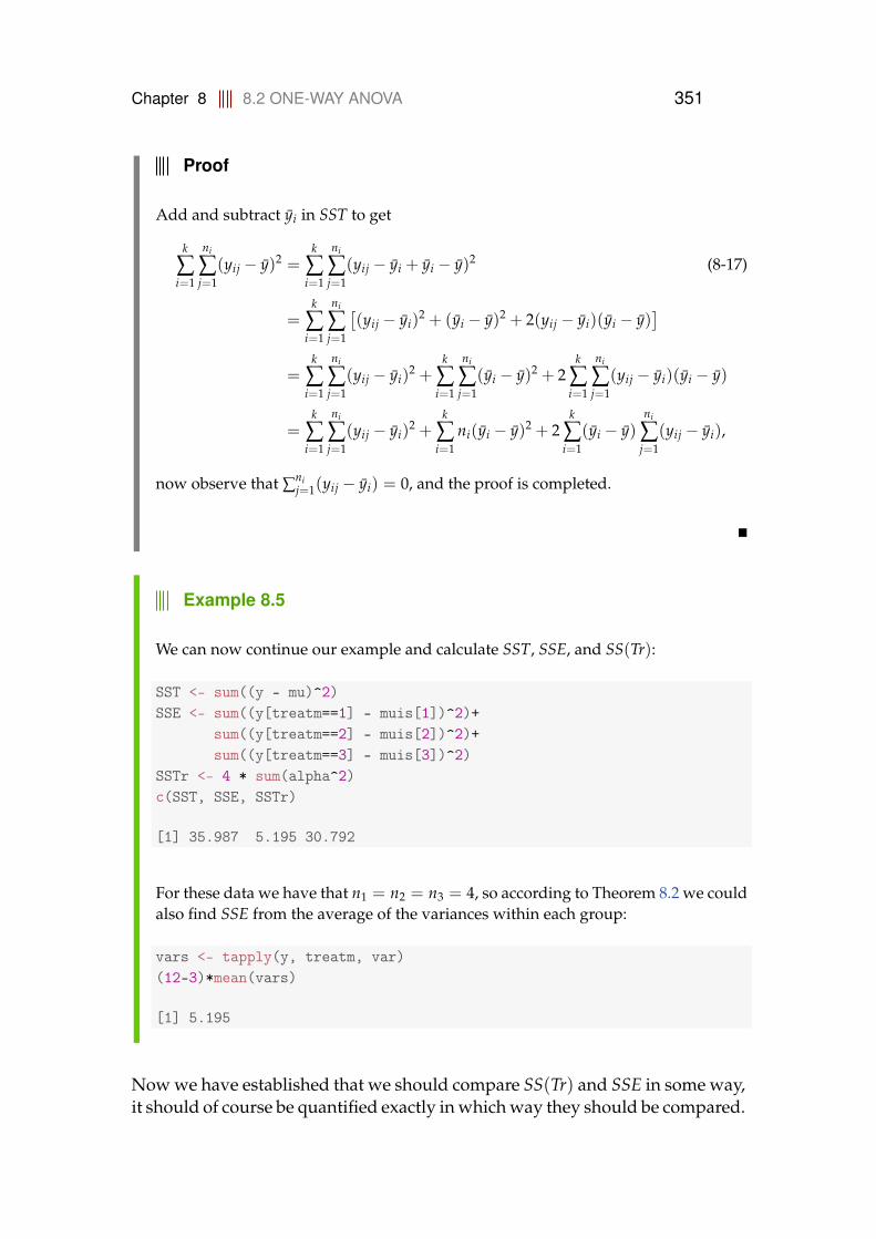
Chapter 8 8.2 ONE-WAY ANOVA 351
Proof
Add and subtract yi in SST to get
k
∑i=1
ni
∑j=1
(yij − y)2 =k
∑i=1
ni
∑j=1
(yij − yi + yi − y)2 (8-17)
=k
∑i=1
ni
∑j=1
[(yij − yi)
2 + (yi − y)2 + 2(yij − yi)(yi − y)]
=k
∑i=1
ni
∑j=1
(yij − yi)2 +
k
∑i=1
ni
∑j=1
(yi − y)2 + 2k
∑i=1
ni
∑j=1
(yij − yi)(yi − y)
=k
∑i=1
ni
∑j=1
(yij − yi)2 +
k
∑i=1
ni(yi − y)2 + 2k
∑i=1
(yi − y)ni
∑j=1
(yij − yi),
now observe that ∑nij=1(yij − yi) = 0, and the proof is completed.
�
Example 8.5
We can now continue our example and calculate SST, SSE, and SS(Tr):
SST <- sum((y - mu)^2)SSE <- sum((y[treatm==1] - muis[1])^2)+
sum((y[treatm==2] - muis[2])^2)+sum((y[treatm==3] - muis[3])^2)
SSTr <- 4 * sum(alpha^2)c(SST, SSE, SSTr)
[1] 35.987 5.195 30.792
For these data we have that n1 = n2 = n3 = 4, so according to Theorem 8.2 we couldalso find SSE from the average of the variances within each group:
vars <- tapply(y, treatm, var)(12-3)*mean(vars)
[1] 5.195
Now we have established that we should compare SS(Tr) and SSE in some way,it should of course be quantified exactly in which way they should be compared.
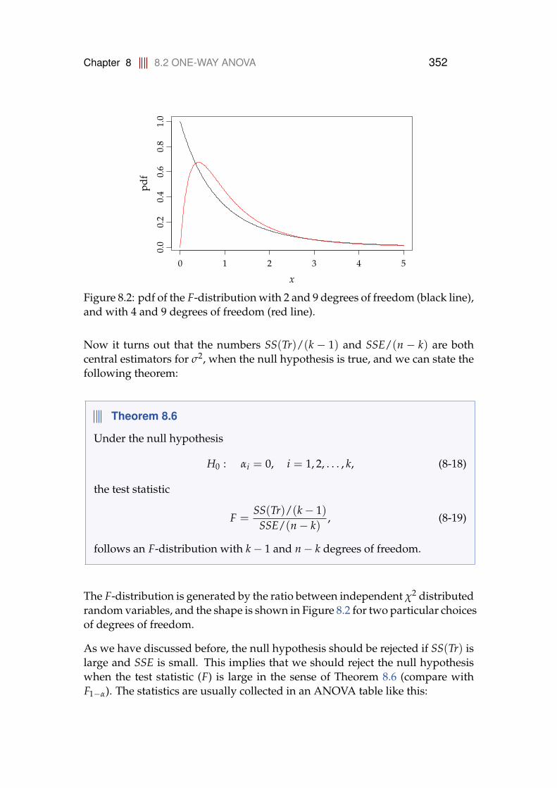
Chapter 8 8.2 ONE-WAY ANOVA 352
0 1 2 3 4 5
0.0
0.2
0.4
0.6
0.8
1.0
x
Figure 8.2: pdf of the F-distribution with 2 and 9 degrees of freedom (black line),and with 4 and 9 degrees of freedom (red line).
Now it turns out that the numbers SS(Tr)/(k − 1) and SSE/(n − k) are bothcentral estimators for σ2, when the null hypothesis is true, and we can state thefollowing theorem:
Theorem 8.6
Under the null hypothesis
H0 : αi = 0, i = 1, 2, . . . , k, (8-18)
the test statistic
F =SS(Tr)/(k− 1)
SSE/(n− k), (8-19)
follows an F-distribution with k− 1 and n− k degrees of freedom.
The F-distribution is generated by the ratio between independent χ2 distributedrandom variables, and the shape is shown in Figure 8.2 for two particular choicesof degrees of freedom.
As we have discussed before, the null hypothesis should be rejected if SS(Tr) islarge and SSE is small. This implies that we should reject the null hypothesiswhen the test statistic (F) is large in the sense of Theorem 8.6 (compare withF1−α). The statistics are usually collected in an ANOVA table like this:

Chapter 8 8.2 ONE-WAY ANOVA 353
Source of Degrees of Sums of Mean sum of Test- p-variation freedom squares squares statistic F valueTreatment k− 1 SS(Tr) MS(Tr) = SS(Tr)
k−1 Fobs =MS(Tr)
MSE P(F > Fobs)
Residual n− k SSE MSE = SSEn−k
Total n− 1 SST
Example 8.7
We can now continue with our example and find the F-statistic and the p-value:
F <- (SSTr/(3 - 1)/(SSE/(12 - 3)))pv <- 1 - pf(F, df1 = 3 - 1, df2 = 12 - 3)c(F , pv)
[1] 26.672281 0.000165
So we have a test statistic F = 26.7 and a p-value equal to 0.000165 and we reject thenull hypothesis on e.g. level α = 0.05. The calculations can of course also be donedirectly in R, by:
anova(lm(y ~ treatm))
Analysis of Variance Table
Response: yDf Sum Sq Mean Sq F value Pr(>F)
treatm 2 30.8 15.40 26.7 0.00017 ***Residuals 9 5.2 0.58---Signif. codes: 0 '***' 0.001 '**' 0.01 '*' 0.05 '.' 0.1 ' ' 1
Note, that in the direct R calculation it is very important to include treatm as a factor,in order to get the correct analysis.
If we reject the null hypothesis, it implies that the observations can be finallydescribed by the initial model re-stated here
Yij = µ + αi + εij, εij ∼ N(0, σ2), (8-20)
and the estimate of σ2 is σ2 = SSE/(n− k) = MSE.
Chapter 8 8.2 ONE-WAY ANOVA 354
Remark 8.8 When multiple groups = 2 groups
When k = 2, that is, we are in the two-sample case studied in Chapter 3, wealready saw above in Theorem 8.4 that MSE = s2
p. Actually, this means thatthe analysis we get from a one-way ANOVA when we apply it for only k = 2groups, which could be perfectly fine - nothing in the ANOVA approachreally relies on k having to be larger than 2 - corresponds to the pooled t-testgiven as Method 3.52. More exact
for k = 2 : Fobs = t2obs, (8-21)
where tobs is the pooled version coming from Methods 3.51 and 3.52. Thusthe p-value obtained from the k = 2 group ANOVA equals exactly the p-value obtained from the pooled t-test given in Method 3.52.
8.2.3 Post hoc comparisons
If we reject the overall null hypothesis above, and hence conclude that αi 6= 0 forat least one i it makes sense to ask which of the treatments are actually different.That is, trying to meet the second of the two major purposes indicated in thebeginning. This can be done by pairwise comparison of the treatments. Wehave already seen in Chapter 3, that such comparison could be based on the t-distribution. We can construct confidence interval with similar formulas exceptthat we should use SSE/(n − k) as the estimate of the residual variance andhence also n− k degrees of freedom in the t-distribution:

Chapter 8 8.2 ONE-WAY ANOVA 355
Method 8.9 Post hoc pairwise confidence intervals
A single pre-planned (1 − α) · 100% confidence interval for the differencebetween treatment i and j is found as
yi − yj ± t1−α/2
√√√√ SSEn− k
(1ni
+1nj
), (8-22)
where t1−α/2 is based on the t-distribution with n− k degrees of freedom.
If all M = k(k − 1)/2 combinations of pairwise confidence intervals arecalculated using the formula M times, but each time with αBonferroni = α/M(see Remark 8.14 below).
Similarly one could do pairwise hypothesis tests:
Method 8.10 Post hoc pairwise hypothesis tests
A single pre-planned level α hypothesis tests:
H0 : µi = µj, H1 : µi 6= µj, (8-23)
is carried out by
tobs =yi − yj√
MSE(
1ni+ 1
nj
) , (8-24)
and
p-value = 2 · P(T > |tobs|), (8-25)
where the t-distribution with n− k degrees of freedom is used.
If all M = k(k− 1)/2 combinations of pairwise hypothesis tests are carriedout use the approach M times but each time with test level αBonferroni = α/M(see Remark 8.14 below).
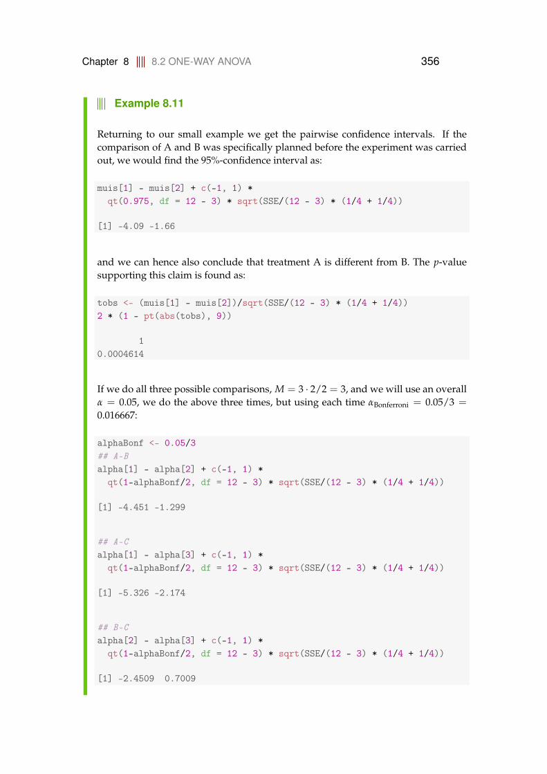
Chapter 8 8.2 ONE-WAY ANOVA 356
Example 8.11
Returning to our small example we get the pairwise confidence intervals. If thecomparison of A and B was specifically planned before the experiment was carriedout, we would find the 95%-confidence interval as:
muis[1] - muis[2] + c(-1, 1) *qt(0.975, df = 12 - 3) * sqrt(SSE/(12 - 3) * (1/4 + 1/4))
[1] -4.09 -1.66
and we can hence also conclude that treatment A is different from B. The p-valuesupporting this claim is found as:
tobs <- (muis[1] - muis[2])/sqrt(SSE/(12 - 3) * (1/4 + 1/4))2 * (1 - pt(abs(tobs), 9))
10.0004614
If we do all three possible comparisons, M = 3 · 2/2 = 3, and we will use an overallα = 0.05, we do the above three times, but using each time αBonferroni = 0.05/3 =
0.016667:
alphaBonf <- 0.05/3## A-Balpha[1] - alpha[2] + c(-1, 1) *
qt(1-alphaBonf/2, df = 12 - 3) * sqrt(SSE/(12 - 3) * (1/4 + 1/4))
[1] -4.451 -1.299
## A-Calpha[1] - alpha[3] + c(-1, 1) *
qt(1-alphaBonf/2, df = 12 - 3) * sqrt(SSE/(12 - 3) * (1/4 + 1/4))
[1] -5.326 -2.174
## B-Calpha[2] - alpha[3] + c(-1, 1) *
qt(1-alphaBonf/2, df = 12 - 3) * sqrt(SSE/(12 - 3) * (1/4 + 1/4))
[1] -2.4509 0.7009
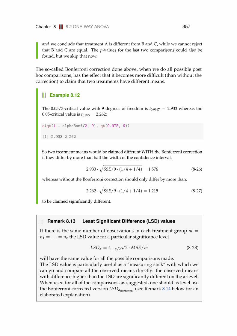
Chapter 8 8.2 ONE-WAY ANOVA 357
and we conclude that treatment A is different from B and C, while we cannot rejectthat B and C are equal. The p-values for the last two comparisons could also befound, but we skip that now.
The so-called Bonferroni correction done above, when we do all possible posthoc comparisons, has the effect that it becomes more difficult (than without thecorrection) to claim that two treatments have different means.
Example 8.12
The 0.05/3-critical value with 9 degrees of freedom is t0.9917 = 2.933 whereas the0.05-critical value is t0.975 = 2.262:
c(qt(1 - alphaBonf/2, 9), qt(0.975, 9))
[1] 2.933 2.262
So two treatment means would be claimed different WITH the Bonferroni correctionif they differ by more than half the width of the confidence interval:
2.933 ·√
SSE/9 · (1/4 + 1/4) = 1.576 (8-26)
whereas without the Bonferroni correction should only differ by more than:
2.262 ·√
SSE/9 · (1/4 + 1/4) = 1.215 (8-27)
to be claimed significantly different.
Remark 8.13 Least Significant Difference (LSD) values
If there is the same number of observations in each treatment group m =n1 = . . . = nk the LSD value for a particular significance level
LSDα = t1−α/2√
2 ·MSE/m (8-28)
will have the same value for all the possible comparisons made.The LSD value is particularly useful as a “measuring stick” with which wecan go and compare all the observed means directly: the observed meanswith difference higher than the LSD are significantly different on the α-level.When used for all of the comparisons, as suggested, one should as level usethe Bonferroni corrected version LSDαBonferroni (see Remark 8.14 below for anelaborated explanation).
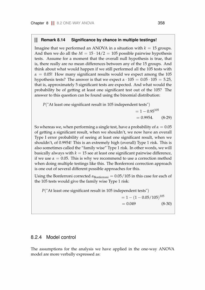
Chapter 8 8.2 ONE-WAY ANOVA 358
Remark 8.14 Significance by chance in multiple testings!
Imagine that we performed an ANOVA in a situation with k = 15 groups.And then we do all the M = 15 · 14/2 = 105 possible pairwise hypothesistests. Assume for a moment that the overall null hypothesis is true, thatis, there really are no mean differences between any of the 15 groups. Andthink about what would happen if we still performed all the 105 tests withα = 0.05! How many significant results would we expect among the 105hypothesis tests? The answer is that we expect α · 105 = 0.05 · 105 = 5.25,that is, approximately 5 significant tests are expected. And what would theprobability be of getting at least one significant test out of the 105? Theanswer to this question can be found using the binomial distribution:
P("At least one significant result in 105 independent tests")
= 1− 0.95105
= 0.9954. (8-29)
So whereas we, when performing a single test, have a probability of α = 0.05of getting a significant result, when we shouldn’t, we now have an overallType I error probability of seeing at least one significant result, when weshouldn’t, of 0.9954! This is an extremely high (overall) Type 1 risk. This isalso sometimes called the “family wise” Type 1 risk. In other words, we willbasically always with k = 15 see at least one significant pairwise difference,if we use α = 0.05. This is why we recommend to use a correction methodwhen doing multiple testings like this. The Bonferroni correction approachis one out of several different possible approaches for this.
Using the Bonferroni corrected αBonferroni = 0.05/105 in this case for each ofthe 105 tests would give the family wise Type 1 risk:
P("At least one significant result in 105 independent tests")
= 1− (1− 0.05/105)105
= 0.049 (8-30)
8.2.4 Model control
The assumptions for the analysis we have applied in the one-way ANOVAmodel are more verbally expressed as:
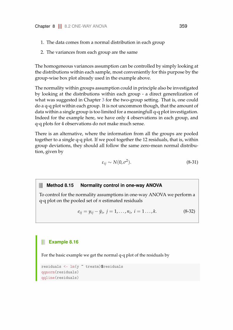
Chapter 8 8.2 ONE-WAY ANOVA 359
1. The data comes from a normal distribution in each group
2. The variances from each group are the same
The homogeneous variances assumption can be controlled by simply looking atthe distributions within each sample, most conveniently for this purpose by thegroup-wise box plot already used in the example above.
The normality within groups assumption could in principle also be investigatedby looking at the distributions within each group - a direct generelization ofwhat was suggested in Chapter 3 for the two-group setting. That is, one coulddo a q-q plot within each group. It is not uncommon though, that the amount ofdata within a single group is too limited for a meaningfull q-q plot investigation.Indeed for the example here, we have only 4 observations in each group, andq-q plots for 4 observations do not make much sense.
There is an alternative, where the information from all the groups are pooledtogether to a single q-q plot. If we pool together the 12 residuals, that is, withingroup deviations, they should all follow the same zero-mean normal distribu-tion, given by
εij ∼ N(0, σ2). (8-31)
Method 8.15 Normality control in one-way ANOVA
To control for the normality assumptions in one-way ANOVA we perform aq-q plot on the pooled set of n estimated residuals
eij = yij − yi, j = 1, . . . , ni, i = 1 . . . , k. (8-32)
Example 8.16
For the basic example we get the normal q-q plot of the residuals by
residuals <- lm(y ~ treatm)$residualsqqnorm(residuals)qqline(residuals)
Chapter 8 8.2 ONE-WAY ANOVA 360
-1.5 -0.5 0.5 1.5
-1.0
-0.5
0.0
0.5
1.0
1.5
Normal Q-Q Plot
Theoretical Quantiles
Sam
ple
Qua
ntile
s
residuals
1 2 3 4 5 6 7 8 9 10-0.225 0.575 0.375 -0.725 -0.400 0.400 0.200 -0.200 -0.975 1.525
11 120.125 -0.675
8.2.5 A complete worked through example: plastic types for lamps
Example 8.17 Plastic types for lamps
On a lamp two plastic screens are to be mounted. It is essential that these plasticscreens have a good impact strength. Therefore an experiment is carried out for 5different types of plastic. 6 samples in each plastic type are tested. The strengths ofthese items are determined. The following measurement data was found (strengthin kJ/m2):
Type of plasticI II III IV V
44.6 52.8 53.1 51.5 48.250.5 58.3 50.0 53.7 40.846.3 55.4 54.4 50.5 44.548.5 57.4 55.3 54.4 43.945.2 58.1 50.6 47.5 45.952.3 54.6 53.4 47.8 42.5

Chapter 8 8.2 ONE-WAY ANOVA 361
We run the following in R:
D <- data.frame(strength=c(44.6, 52.8, 53.1, 51.5, 48.2, 50.5, 58.3, 50.0, 53.7, 40.8,
46.3, 55.4, 54.4, 50.5, 44.5, 48.5, 57.4, 55.3, 54.4, 43.9,45.2, 58.1, 50.6, 47.5, 45.9, 52.3, 54.6, 53.4, 47.8, 42.5),
plastictype=factor(rep(1:5, 6)))plot(D$plastictype, D$strength, xlab="Plastictype", ylab="Strength")
1 2 3 4 5
4550
55
Plastictype
Stre
ngth
fit <- lm(strength ~ plastictype, data=D)anova(fit)
Analysis of Variance Table
Response: strengthDf Sum Sq Mean Sq F value Pr(>F)
plastictype 4 492 122.9 18.2 4e-07 ***Residuals 25 169 6.7---Signif. codes: 0 '***' 0.001 '**' 0.01 '*' 0.05 '.' 0.1 ' ' 1
The ANOVA results are more nicely put in a table here:
Df Sum Sq Mean Sq F value Pr(>F)Plastictype 4 491.76 122.94 18.23 4 · 10−7
Residuals 25 168.56 6.74
From the box plot we see that there appears to be group mean differences and ex-tremely low p-value in the ANOVA table confirms this: there is very strong evidence
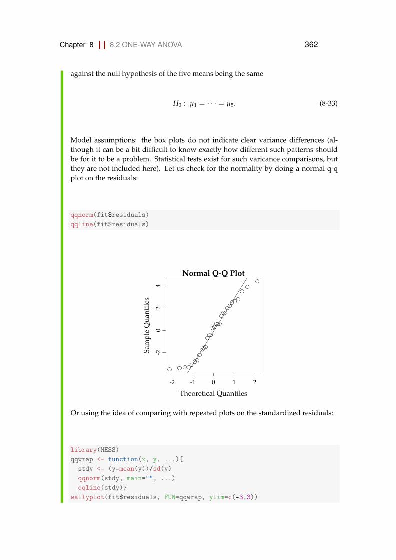
Chapter 8 8.2 ONE-WAY ANOVA 362
against the null hypothesis of the five means being the same
H0 : µ1 = · · · = µ5. (8-33)
Model assumptions: the box plots do not indicate clear variance differences (al-though it can be a bit difficult to know exactly how different such patterns shouldbe for it to be a problem. Statistical tests exist for such varicance comparisons, butthey are not included here). Let us check for the normality by doing a normal q-qplot on the residuals:
qqnorm(fit$residuals)qqline(fit$residuals)
-2 -1 0 1 2
-20
24
Normal Q-Q Plot
Theoretical Quantiles
Sam
ple
Qua
ntile
s
Or using the idea of comparing with repeated plots on the standardized residuals:
library(MESS)qqwrap <- function(x, y, ...){
stdy <- (y-mean(y))/sd(y)qqnorm(stdy, main="", ...)qqline(stdy)}
wallyplot(fit$residuals, FUN=qqwrap, ylim=c(-3,3))

Chapter 8 8.2 ONE-WAY ANOVA 363
-2 -1 0 1 2
-3-2
-10
12
3
Theoretical Quantiles
Sam
ple
Qua
ntile
s
-2 -1 0 1 2
-3-2
-10
12
3
Theoretical Quantiles
Sam
ple
Qua
ntile
s
-2 -1 0 1 2
-3-2
-10
12
3
Theoretical Quantiles
Sam
ple
Qua
ntile
s
-2 -1 0 1 2
-3-2
-10
12
3
Theoretical Quantiles
Sam
ple
Qua
ntile
s
-2 -1 0 1 2
-3-2
-10
12
3
Theoretical Quantiles
Sam
ple
Qua
ntile
s
-2 -1 0 1 2
-3-2
-10
12
3
Theoretical Quantiles
Sam
ple
Qua
ntile
s
-2 -1 0 1 2
-3-2
-10
12
3
Theoretical Quantiles
Sam
ple
Qua
ntile
s
-2 -1 0 1 2
-3-2
-10
12
3
Theoretical Quantiles
Sam
ple
Qua
ntile
s
-2 -1 0 1 2
-3-2
-10
12
3
Theoretical Quantiles
Sam
ple
Qua
ntile
s
There appears to be no important deviation from normality.
To complete the story about (quantifying) the five plastic types, we first compute thefive means:
tapply(D$strength, D$plastictype, mean)
1 2 3 4 547.9 56.1 52.8 50.9 44.3
And then we want to construct the M = 5 · 4/2 = 10 different confidence intervalsusing Method 8.9. As all nis equal 6 in this case, all 10 confidence intervals will havethe same width, and we can use Remark 8.13 and compute the (half) width of theconfidence intervals, the LSD-value. And since there are 10 multiple comparisonswe will use αBonferroni = 0.05/10 = 0.005:

Chapter 8 8.3 TWO-WAY ANOVA 364
LSD_0.005 <- qt(0.9975, 25) * sqrt(2*6.74/6)LSD_0.005
[1] 4.614
So Plastictypes are significantly different from each other if they differ by more than4.61. A convenient way to collect the information about the 10 comparisons is byordering the means from smallest to largest and then using the so-called compactletter display:
Plastictype Mean5 44.3 a1 47.9 ab4 50.9 bc3 52.8 cd2 56.1 d
Plastic types with a mean difference less than the LSD-value, hence not significantlydifferent share letters. Plastic types not sharing letters are significantly different. Wecan hence read off all the 10 comparisons from this table.
One could also add the compact letter information to the boxplot for a nice plotting -it is allowed to be creative (while not changing the basic information and the results!)in order to communicate the results.
8.3 Two-way ANOVA
8.3.1 Data structure and model
The one-way ANOVA is the natural multi-sample extension of the indepen-dent two-sample situation covered in Section 3.2. The k samples are hence com-pletely independent from each other, which e.g. in a clinical experiment wouldmean that different patients get different treatments – and hence each patientonly tries a single treatment. Often this would be the only possible way to do acomparison of treatments.
However, sometimes it will be possible to apply multiple treatments to the samepatient (with some time in between). This could then lead to a multi-treatmentsetup, where the sample within each treatment consists of the same patients.This is the natural extension of the paired-design setup covered in Section 3.2.3,where we “pair” if there is exactly 2 treatments. With more than two treatmentswe use the phrase “block”. A block would then be the patient in this case -

Chapter 8 8.3 TWO-WAY ANOVA 365
and the same blocks then appear in all treatment samples. The “block” namecomes from the historical background of these methods coming from agricul-tural field trials, where a block would be an actual piece of land within whichall treatments are applied.
Remark 8.18 Design: independent sampling or blocking?
For the project manager who is in charge of designing the study there willbe a choice to make in cases where both approaches are practicle feasible:should the independent samples approach or the blocked approach be used?Should we use, say, 4 groups of 20 patients each, that is 80 patients all to-gether, or should we use the same 20 patients in each of the four groups?The costs would probably be more or less the same. It sounds nice with 80patients rather than 20? However, the answer is actually pretty clear if what-ever we are going to measure will vary importantly from person to person.And most things in medical studies do vary a lot from person to person dueto many things: gender, age, weight, BMI, or simply due to genetic differ-ences that means that our bodies will respond differently to the medicin.Then the blocked design would definitely be the better choice! This is so,as we will see below, in the analysis of the blocked design the block-main-variability is accounted for and will not “blur” the treatment difference sig-nal. In the independent design the person-to-person variability may be themain part of the “within group” varibility used for the statistical analysis.Or differently put: in a block design each patient would act as his/her owncontrol, the treatment comparison is carried out “within the block”.
For the actual study design it would in both cases be recommended to ran-domize the allocation of patients as much as possible: In the independentdesign patients should be allocated to treatments by randomization. In theblock design all patients receive all treatments but then one would random-ize the order in which they receive the treatments. For this reason these twotypes of expereimental designs are usually called the Completely RandomizedDesign and the Randomized Block Design.
We looked above in the one-way part at an example with 3 treatments with4 observations for each. If the observations were on 4 different persons (andnot 12) it would make sense and would be important to include this personvariability in the model. The resulting model becomes:
Yij = µ + αi + β j + εij, εij ∼ N(0, σ2), (8-34)
so there is an overall mean µ, a treatment effect αi and a block effect β j and ourusual random error term εij.

Chapter 8 8.3 TWO-WAY ANOVA 366
The design is illustrated in the table below, so we have k treatments (A1, . . . ,Ak)and l blocks (B1, . . . ,Bl):
B1 . . . BlA1 y11 . . . y1,l...
... . . ....
Ak yk,1 . . . yk,l
We can now find the parameters in the model above by
µ =1
k · lk
∑i=1
l
∑j=1
yij, (8-35)
αi =
(1l
l
∑j=1
yij
)− µ, (8-36)
β j =
(1k
k
∑i=1
yij
)− µ. (8-37)
Or expressed more compact, with the definitions of the terms obvious from theabove:
µ = ¯y, (8-38)αi = yi· − ¯y, (8-39)
β j = y·j − ¯y. (8-40)
In a way, these means are the essential information in these data. All the rest wedo is just all the statistics to distinguish signal from noise. It does not changethe fact, that these means contain the core story. It also shows explicitly how wenow compute means, not only across one way in the data table, but also acrossthe other way. We compute means both row-wise and column-wise. Hence thename: two-way ANOVA.
Example 8.19
Lets assume that the data we used in the previous section was actually a result of arandomized block design and we could therefore write:
Group A Group B Group CBlock 1 2.8 5.5 5.8Block 2 3.6 6.3 8.3Block 3 3.4 6.1 6.9Block 4 2.3 5.7 6.1
Chapter 8 8.3 TWO-WAY ANOVA 367
In this case we should of course keep track of the blocks as well as the treatments:
y <- c(2.8, 3.6, 3.4, 2.3,5.5, 6.3, 6.1, 5.7,5.8, 8.3, 6.9, 6.1)
treatm <- factor(c(1, 1, 1, 1,2, 2, 2, 2,3, 3, 3, 3))
block <- factor(c(1, 2, 3, 4,1, 2, 3, 4,1, 2, 3, 4))
Now we can calculate the parameter estimates (µ and αi, and β j):
mu <- mean(y)alpha <- tapply(y, treatm, mean) - mubeta <- tapply(y, block, mean) - mumu
[1] 5.233
alpha
1 2 3-2.2083 0.6667 1.5417
beta
1 2 3 4-0.5333 0.8333 0.2333 -0.5333
so our estimates of the overall mean (µ) and αi remain the same while the estimatedblock effects are β1 = −0.53, β2 = 0.83, β3 = 0.23 and β4 = −0.53.
8.3.2 Decomposition of variability and the ANOVA table
In the same way as we saw for the one-way ANOVA, there exists a decomposi-tion of variation for the two-way ANOVA:
Chapter 8 8.3 TWO-WAY ANOVA 368
Theorem 8.20 Variation decomposition
The total sum of squares (SST) can be decomposed into sum of squarederrors (SSE), treatment sum of squares (SS(Tr)), and a block sum of squares(SS(Bl))
k
∑i=1
l
∑j=1
(yij − µ)2
︸ ︷︷ ︸SST
=k
∑i=1
l
∑j=1
(yij − αi − β j − µ)2
︸ ︷︷ ︸SSE
+ l ·k
∑i=1
α2i
︸ ︷︷ ︸SS(Tr)
+ k ·l
∑j=1
β2j
︸ ︷︷ ︸SS(Bl)
=k
∑i=1
l
∑j=1
(yij − yi· − y·j + ¯y)2
︸ ︷︷ ︸SSE
+ l ·k
∑i=1
(yi· − ¯y)2
︸ ︷︷ ︸SS(Tr)
+ k ·l
∑j=1
(y·j − ¯y)2
︸ ︷︷ ︸SS(Bl)
,
(8-41)
Expressed in short form
SST = SS(Tr) + SS(Bl) + SSE. (8-42)
Note, how the SST and SS(Tr) are found exactly as in the one-way ANOVA.If one ignores the block-way of the table, the two-way data has exactly thesame structure as one-way data (with the same number of observations in eachgroup). Further, note how SS(Bl) corresponds to finding a “one-way SS(Tr)”,but on the other way of the table (and ignoring the treatment-way of the datatable). So from a computational point of view, finding these three, that is, find-ing SST, SS(Tr) and SS(Bl) is done by known one-way methodology. And thenthe last one, SSE, could then be found from the decomposition theorem as:
SSE = SST− SS(Tr)− SS(Bl). (8-43)
Example 8.21
Returning to the example we get (SST and SS(Tr) remain unchanged):
SSBl <- 3 * sum(beta^2)SSE <- SST - SSTr - SSBlc(SST, SSE, SSTr, SSBl)
[1] 35.987 1.242 30.792 3.953
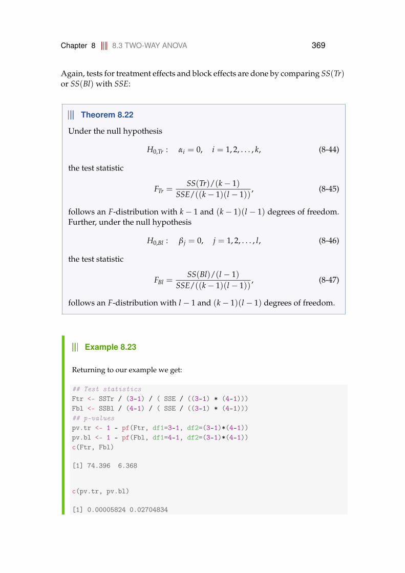
Chapter 8 8.3 TWO-WAY ANOVA 369
Again, tests for treatment effects and block effects are done by comparing SS(Tr)or SS(Bl) with SSE:
Theorem 8.22
Under the null hypothesis
H0,Tr : αi = 0, i = 1, 2, . . . , k, (8-44)
the test statistic
FTr =SS(Tr)/(k− 1)
SSE/((k− 1)(l − 1)), (8-45)
follows an F-distribution with k− 1 and (k− 1)(l − 1) degrees of freedom.Further, under the null hypothesis
H0,Bl : β j = 0, j = 1, 2, . . . , l, (8-46)
the test statistic
FBl =SS(Bl)/(l − 1)
SSE/((k− 1)(l − 1)), (8-47)
follows an F-distribution with l − 1 and (k− 1)(l − 1) degrees of freedom.
Example 8.23
Returning to our example we get:
## Test statisticsFtr <- SSTr / (3-1) / ( SSE / ((3-1) * (4-1)))Fbl <- SSBl / (4-1) / ( SSE / ((3-1) * (4-1)))## p-valuespv.tr <- 1 - pf(Ftr, df1=3-1, df2=(3-1)*(4-1))pv.bl <- 1 - pf(Fbl, df1=4-1, df2=(3-1)*(4-1))c(Ftr, Fbl)
[1] 74.396 6.368
c(pv.tr, pv.bl)
[1] 0.00005824 0.02704834
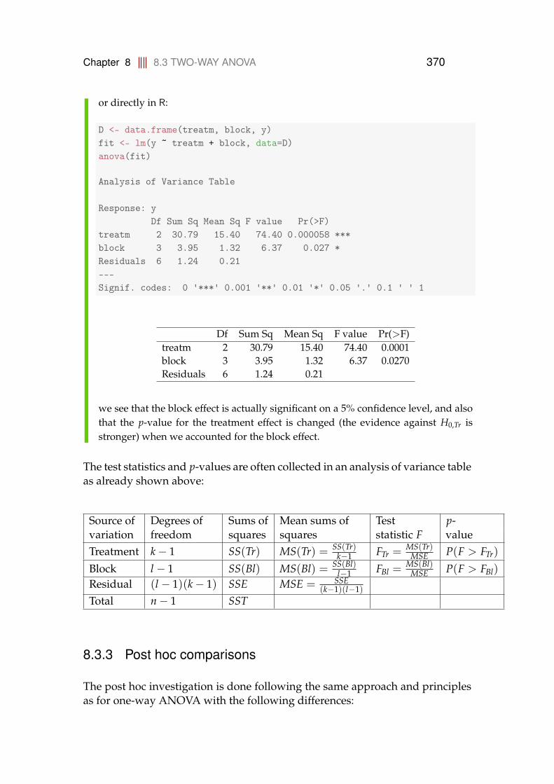
Chapter 8 8.3 TWO-WAY ANOVA 370
or directly in R:
D <- data.frame(treatm, block, y)fit <- lm(y ~ treatm + block, data=D)anova(fit)
Analysis of Variance Table
Response: yDf Sum Sq Mean Sq F value Pr(>F)
treatm 2 30.79 15.40 74.40 0.000058 ***block 3 3.95 1.32 6.37 0.027 *Residuals 6 1.24 0.21---Signif. codes: 0 '***' 0.001 '**' 0.01 '*' 0.05 '.' 0.1 ' ' 1
Df Sum Sq Mean Sq F value Pr(>F)treatm 2 30.79 15.40 74.40 0.0001block 3 3.95 1.32 6.37 0.0270Residuals 6 1.24 0.21
we see that the block effect is actually significant on a 5% confidence level, and alsothat the p-value for the treatment effect is changed (the evidence against H0,Tr isstronger) when we accounted for the block effect.
The test statistics and p-values are often collected in an analysis of variance tableas already shown above:
Source of Degrees of Sums of Mean sums of Test p-variation freedom squares squares statistic F valueTreatment k− 1 SS(Tr) MS(Tr) = SS(Tr)
k−1 FTr =MS(Tr)
MSE P(F > FTr)
Block l − 1 SS(Bl) MS(Bl) = SS(Bl)l−1 FBl =
MS(Bl)MSE P(F > FBl)
Residual (l − 1)(k− 1) SSE MSE = SSE(k−1)(l−1)
Total n− 1 SST
8.3.3 Post hoc comparisons
The post hoc investigation is done following the same approach and principlesas for one-way ANOVA with the following differences:
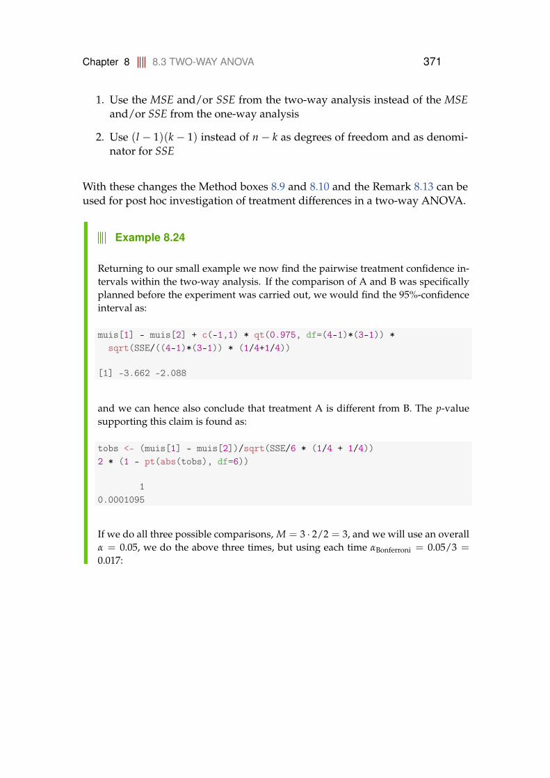
Chapter 8 8.3 TWO-WAY ANOVA 371
1. Use the MSE and/or SSE from the two-way analysis instead of the MSEand/or SSE from the one-way analysis
2. Use (l − 1)(k− 1) instead of n− k as degrees of freedom and as denomi-nator for SSE
With these changes the Method boxes 8.9 and 8.10 and the Remark 8.13 can beused for post hoc investigation of treatment differences in a two-way ANOVA.
Example 8.24
Returning to our small example we now find the pairwise treatment confidence in-tervals within the two-way analysis. If the comparison of A and B was specificallyplanned before the experiment was carried out, we would find the 95%-confidenceinterval as:
muis[1] - muis[2] + c(-1,1) * qt(0.975, df=(4-1)*(3-1)) *sqrt(SSE/((4-1)*(3-1)) * (1/4+1/4))
[1] -3.662 -2.088
and we can hence also conclude that treatment A is different from B. The p-valuesupporting this claim is found as:
tobs <- (muis[1] - muis[2])/sqrt(SSE/6 * (1/4 + 1/4))2 * (1 - pt(abs(tobs), df=6))
10.0001095
If we do all three possible comparisons, M = 3 · 2/2 = 3, and we will use an overallα = 0.05, we do the above three times, but using each time αBonferroni = 0.05/3 =
0.017:
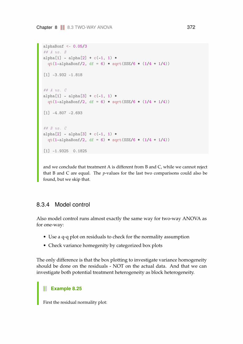
Chapter 8 8.3 TWO-WAY ANOVA 372
alphaBonf <- 0.05/3## A vs. Balpha[1] - alpha[2] + c(-1, 1) *
qt(1-alphaBonf/2, df = 6) * sqrt(SSE/6 * (1/4 + 1/4))
[1] -3.932 -1.818
## A vs. Calpha[1] - alpha[3] + c(-1, 1) *
qt(1-alphaBonf/2, df = 6) * sqrt(SSE/6 * (1/4 + 1/4))
[1] -4.807 -2.693
## B vs. Calpha[2] - alpha[3] + c(-1, 1) *
qt(1-alphaBonf/2, df = 6) * sqrt(SSE/6 * (1/4 + 1/4))
[1] -1.9325 0.1825
and we conclude that treatment A is different from B and C, while we cannot rejectthat B and C are equal. The p-values for the last two comparisons could also befound, but we skip that.
8.3.4 Model control
Also model control runs almost exactly the same way for two-way ANOVA asfor one-way:
• Use a q-q plot on residuals to check for the normality assumption
• Check variance homegenity by categorized box plots
The only difference is that the box plotting to investigate variance homogeneityshould be done on the residuals - NOT on the actual data. And that we caninvestigate both potential treatment heterogeneity as block heterogeneity.
Example 8.25
First the residual normality plot:
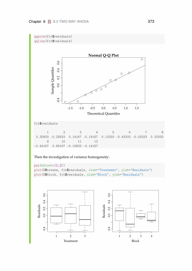
Chapter 8 8.3 TWO-WAY ANOVA 373
qqnorm(fit$residuals)qqline(fit$residuals)
-1.5 -1.0 -0.5 0.0 0.5 1.0 1.5
-0.4
0.0
0.2
0.4
0.6
Normal Q-Q Plot
Theoretical Quantiles
Sam
ple
Qua
ntile
s
fit$residuals
1 2 3 4 5 6 7 80.30833 -0.25833 0.14167 -0.19167 0.13333 -0.43333 -0.03333 0.33333
9 10 11 12-0.44167 0.69167 -0.10833 -0.14167
Then the investigation of variance homogeneity:
par(mfrow=c(1,2))plot(D$treatm, fit$residuals, xlab="Treatment", ylab="Residuals")plot(D$block, fit$residuals, xlab="Block", ylab="Residuals")
1 2 3
-0.4
0.0
0.2
0.4
0.6
Treatment
Res
idua
ls
1 2 3 4
-0.4
0.0
0.2
0.4
0.6
Block
Res
idua
ls
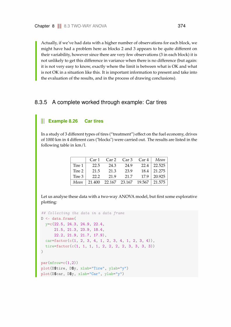
Chapter 8 8.3 TWO-WAY ANOVA 374
Actually, if we’ve had data with a higher number of observations for each block, wemight have had a problem here as blocks 2 and 3 appears to be quite different ontheir variability, however since there are very few observations (3 in each block) it isnot unlikely to get this difference in variance when there is no difference (but again:it is not very easy to know, exactly where the limit is between what is OK and whatis not OK in a situation like this. It is important information to present and take intothe evaluation of the results, and in the process of drawing conclusions).
8.3.5 A complete worked through example: Car tires
Example 8.26 Car tires
In a study of 3 different types of tires (“treatment”) effect on the fuel economy, drivesof 1000 km in 4 different cars ("blocks") were carried out. The results are listed in thefollowing table in km/l.
Car 1 Car 2 Car 3 Car 4 MeanTire 1 22.5 24.3 24.9 22.4 22.525Tire 2 21.5 21.3 23.9 18.4 21.275Tire 3 22.2 21.9 21.7 17.9 20.925Mean 21.400 22.167 23.167 19.567 21.575
Let us analyse these data with a two-way ANOVA model, but first some explorativeplotting:
## Collecting the data in a data frameD <- data.frame(
y=c(22.5, 24.3, 24.9, 22.4,21.5, 21.3, 23.9, 18.4,22.2, 21.9, 21.7, 17.9),
car=factor(c(1, 2, 3, 4, 1, 2, 3, 4, 1, 2, 3, 4)),tire=factor(c(1, 1, 1, 1, 2, 2, 2, 2, 3, 3, 3, 3))
)
par(mfrow=c(1,2))plot(D$tire, D$y, xlab="Tire", ylab="y")plot(D$car, D$y, xlab="Car", ylab="y")
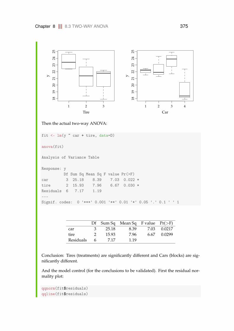
Chapter 8 8.3 TWO-WAY ANOVA 375
1 2 3
1819
2021
2223
2425
Tire
y
1 2 3 4
1819
2021
2223
2425
Car
yThen the actual two-way ANOVA:
fit <- lm(y ~ car + tire, data=D)
anova(fit)
Analysis of Variance Table
Response: yDf Sum Sq Mean Sq F value Pr(>F)
car 3 25.18 8.39 7.03 0.022 *tire 2 15.93 7.96 6.67 0.030 *Residuals 6 7.17 1.19---Signif. codes: 0 '***' 0.001 '**' 0.01 '*' 0.05 '.' 0.1 ' ' 1
Df Sum Sq Mean Sq F value Pr(>F)car 3 25.18 8.39 7.03 0.0217tire 2 15.93 7.96 6.67 0.0299Residuals 6 7.17 1.19
Conclusion: Tires (treatments) are significantly different and Cars (blocks) are sig-nificantly different.
And the model control (for the conclusions to be validated). First the residual nor-mality plot:
qqnorm(fit$residuals)qqline(fit$residuals)

Chapter 8 8.3 TWO-WAY ANOVA 376
-1.5 -0.5 0.5 1.5
-1.0
-0.5
0.0
0.5
1.0
Normal Q-Q Plot
Theoretical Quantiles
Sam
ple
Qua
ntile
s
Then the investigation of variance homogeneity:
par(mfrow=c(1,2))plot(D$car, fit$residuals, xlab="Car", ylab="Residuals")plot(D$tire, fit$residuals, xlab="Tire", ylab="Residuals")
1 2 3 4
-1.0
-0.5
0.0
0.5
1.0
Car
Res
idua
ls
1 2 3
-1.0
-0.5
0.0
0.5
1.0
Tire
Res
idua
ls
It seems like the variance for Car 2 and Car 3 is difference, however, as in the previ-ous example, there are very few observations (only 3) for each car, hence this differ-ence in variation is not unlikely if there is no difference. Thus we find that there donot see any important deviations from the model assumptions.
Finally, the post hoc analysis, first the treatment means:
tapply(D$y, D$tire, mean)
1 2 323.52 21.27 20.92
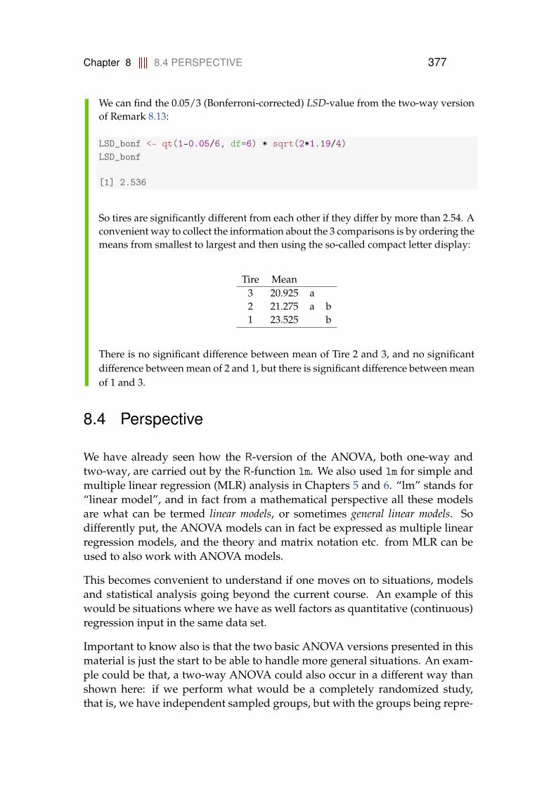
Chapter 8 8.4 PERSPECTIVE 377
We can find the 0.05/3 (Bonferroni-corrected) LSD-value from the two-way versionof Remark 8.13:
LSD_bonf <- qt(1-0.05/6, df=6) * sqrt(2*1.19/4)LSD_bonf
[1] 2.536
So tires are significantly different from each other if they differ by more than 2.54. Aconvenient way to collect the information about the 3 comparisons is by ordering themeans from smallest to largest and then using the so-called compact letter display:
Tire Mean3 20.925 a2 21.275 a b1 23.525 b
There is no significant difference between mean of Tire 2 and 3, and no significantdifference between mean of 2 and 1, but there is significant difference between meanof 1 and 3.
8.4 Perspective
We have already seen how the R-version of the ANOVA, both one-way andtwo-way, are carried out by the R-function lm. We also used lm for simple andmultiple linear regression (MLR) analysis in Chapters 5 and 6. “lm” stands for“linear model”, and in fact from a mathematical perspective all these modelsare what can be termed linear models, or sometimes general linear models. Sodifferently put, the ANOVA models can in fact be expressed as multiple linearregression models, and the theory and matrix notation etc. from MLR can beused to also work with ANOVA models.
This becomes convenient to understand if one moves on to situations, modelsand statistical analysis going beyond the current course. An example of thiswould be situations where we have as well factors as quantitative (continuous)regression input in the same data set.
Important to know also is that the two basic ANOVA versions presented in thismaterial is just the start to be able to handle more general situations. An exam-ple could be that, a two-way ANOVA could also occur in a different way thanshown here: if we perform what would be a completely randomized study,that is, we have independent sampled groups, but with the groups being repre-

Chapter 8 8.4 PERSPECTIVE 378
sented by a two-way treatment factor structure, say, factor A with 5 levels andfactor B with 3 levels. Hence, we have all 15 groups consisting of all combina-tions of the two treatments, but with several observations within each of the 15groups. This would sometimes be called a two-way ANOVA with replications,whereas the randomized block setting covered above then would be the two-way ANOVA without replication (there is only and exactly one observation foreach combination of treatment and block).
And then the next step could be even more than two treatment factors, andmaybe such a multi-factorial setting could even be combined with blocking andmaybe some quantitative x-input (then often called covariates) calling for ex-tentions of all this.
Another important extension direction are situations with different levels of ob-servations/variability: there could be hierarchical structures in the data, e.g.repeated measurents on an individual animal, but having also many animals inthe study, and animals might come from different farms, that lies in differentregions within different countries. This calls for so-called hierarchical models,multi-level models, variance components models or models, where both treat-ment factors and such hierarchical random effects are present – the so-calledmixed models.
All of this and many other good things can be learned in statistics courses build-ing further on the methods presented in this material!

Chapter 8 8.5 EXERCISES 379
8.5 Exercises
Exercise 8.1 Environment action plans
To investigate the effect of two recent national Danish aquatic environment ac-tion plans the concentration of nitrogen (measured in g/m3) have been mea-sured in a particular river just before the national action plans were enforced(1998 and 2003) and in 2011. Each measurement is repeated 6 times during ashort stretch of river. The result is shown in the following table:
N1998 N2003 N20115.01 5.59 3.026.23 5.13 4.765.98 5.33 3.465.31 4.65 4.125.13 5.52 4.515.65 4.92 4.42
Row mean 5.5517 5.1900 4.0483
Further, the total variation in the data is SST = 11.4944. You got the followingoutput from R corresponding to a one-way analysis of variance (where most ofthe information, however, is replaced by the letters A-E as well as U and V):
> anova(lm(N ~ Year))Analysis of Variance Table
Response: NDf SumSq MeanSq Fvalue Pr(>F)
Year A B C U VResiduals D 4.1060 E
a) What numbers did the letters A-D substitute?
b) If you use the significance level α = 0.05, what critical value should beused for the hypothesis test carried out in the analysis (and in the tableillustrated with the figures U and V)?
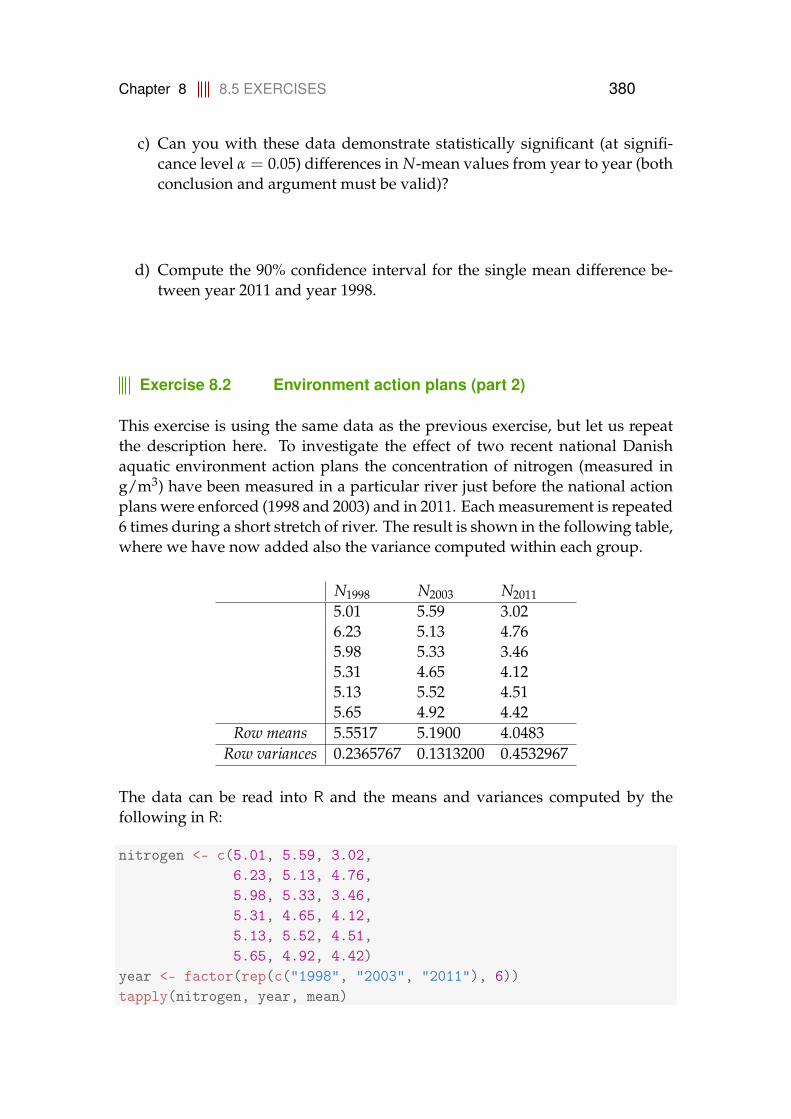
Chapter 8 8.5 EXERCISES 380
c) Can you with these data demonstrate statistically significant (at signifi-cance level α = 0.05) differences in N-mean values from year to year (bothconclusion and argument must be valid)?
d) Compute the 90% confidence interval for the single mean difference be-tween year 2011 and year 1998.
Exercise 8.2 Environment action plans (part 2)
This exercise is using the same data as the previous exercise, but let us repeatthe description here. To investigate the effect of two recent national Danishaquatic environment action plans the concentration of nitrogen (measured ing/m3) have been measured in a particular river just before the national actionplans were enforced (1998 and 2003) and in 2011. Each measurement is repeated6 times during a short stretch of river. The result is shown in the following table,where we have now added also the variance computed within each group.
N1998 N2003 N20115.01 5.59 3.026.23 5.13 4.765.98 5.33 3.465.31 4.65 4.125.13 5.52 4.515.65 4.92 4.42
Row means 5.5517 5.1900 4.0483Row variances 0.2365767 0.1313200 0.4532967
The data can be read into R and the means and variances computed by thefollowing in R:
nitrogen <- c(5.01, 5.59, 3.02,6.23, 5.13, 4.76,5.98, 5.33, 3.46,5.31, 4.65, 4.12,5.13, 5.52, 4.51,5.65, 4.92, 4.42)
year <- factor(rep(c("1998", "2003", "2011"), 6))tapply(nitrogen, year, mean)

Chapter 8 8.5 EXERCISES 381
1998 2003 20115.552 5.190 4.048
tapply(nitrogen, year, var)
1998 2003 20110.2366 0.1313 0.4533
mean(nitrogen)
[1] 4.93
a) Compute the three sums of squares (SST, SS(Tr) and SSE) using the threemeans and three variances, and the overall mean (show the formulas ex-plicitly).
b) Find the SST-value in R using the sample variance function var.
c) Run the ANOVA in R and produce the ANOVA table in R.
d) Do a complete post hoc analysis, where all the 3 years are compared pair-wise.
e) Use R to do model validation by residual analysis.

Chapter 8 8.5 EXERCISES 382
Exercise 8.3 Plastic film
A company is starting a production of a new type of patch. For the product athin plastic film is to be used. Samples of products were received from 5 possiblesuppliers. Each sample consisted of 20 measurements of the film thickness andthe following data were found:
Average film thickness Sample standard deviationx in µm s in µm
Supplier 1 31.4 1.9Supplier 2 30.6 1.6Supplier 3 30.5 2.2Supplier 4 31.3 1.8Supplier 5 29.2 2.2
From the usual calculations for a one-way analysis of variance the following isobtained:
Source Degrees of freedom Sums of SquaresSupplier 4 SS(Tr) = 62Error 95 SSE = 362.71
a) Is there a significant (α = 5%) difference between the mean film thick-nesses for the suppliers (both conclusion and argument must be correct)?
b) Compute a 95% confidence interval for the difference in mean film thick-nesses of Supplier 1 and Supplier 4 (considered as a “single pre-planned”comparison).
Exercise 8.4 Brass alloys
When brass is used in a production, the modulus of elasticity, E, of the materialis often important for the functionality. The modulus of elasticity for 6 differentbrass alloys are measured. 5 samples from each alloy are tested. The results areshown in the table below where the measured modulus of elasticity is given inGPa:
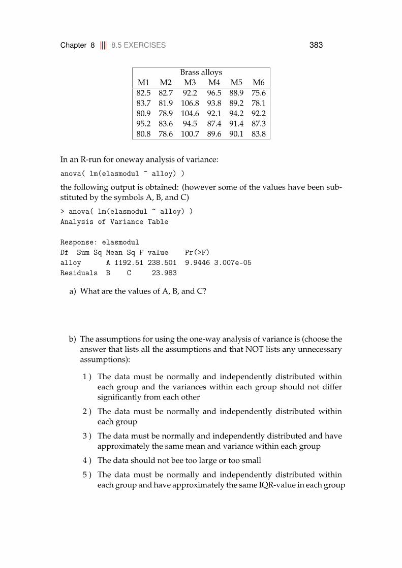
Chapter 8 8.5 EXERCISES 383
Brass alloysM1 M2 M3 M4 M5 M682.5 82.7 92.2 96.5 88.9 75.683.7 81.9 106.8 93.8 89.2 78.180.9 78.9 104.6 92.1 94.2 92.295.2 83.6 94.5 87.4 91.4 87.380.8 78.6 100.7 89.6 90.1 83.8
In an R-run for oneway analysis of variance:
anova( lm(elasmodul ~ alloy) )
the following output is obtained: (however some of the values have been sub-stituted by the symbols A, B, and C)
> anova( lm(elasmodul ~ alloy) )Analysis of Variance Table
Response: elasmodulDf Sum Sq Mean Sq F value Pr(>F)alloy A 1192.51 238.501 9.9446 3.007e-05Residuals B C 23.983
a) What are the values of A, B, and C?
b) The assumptions for using the one-way analysis of variance is (choose theanswer that lists all the assumptions and that NOT lists any unnecessaryassumptions):
1 ) The data must be normally and independently distributed withineach group and the variances within each group should not differsignificantly from each other
2 ) The data must be normally and independently distributed withineach group
3 ) The data must be normally and independently distributed and haveapproximately the same mean and variance within each group
4 ) The data should not bee too large or too small
5 ) The data must be normally and independently distributed withineach group and have approximately the same IQR-value in each group
Chapter 8 8.5 EXERCISES 384
c) Compute a 95% confidence interval for the single pre-planned differencebetween brass alloy 1 and 2.
Exercise 8.5 Plastic tubes
Some plastic tubes for which the tensile strength is essential are to be produced.Hence, sample tube items are produced and tested, where the tensile strengthis determined. Two different granules and four possible suppliers are used inthe trial. The measurement results (in MPa) from the trial are listed in the tablebelow:
Granuleg1 g2
Supplier a 34.2 33.1Supplier b 34.8 31.2Supplier c 31.3 30.2Supplier d 31.9 31.6
The following is run in R:
D <- data.frame(strength=c(34.2,34.8,31.3,31.9,33.1,31.2,30.2,31.6),supplier=factor(c("a","b","c","d","a","b","c","d")),granule=factor(c(1,1,1,1,2,2,2,2))
)anova(lm( strength ~ supplier + granule, data=D))
with the following result:

Chapter 8 8.5 EXERCISES 385
Analysis of Variance Table
Response: strengthDf Sum Sq Mean Sq F value Pr(>F)
supplier 3 10.0338 3.3446 3.2537 0.1792granule 1 4.6512 4.6512 4.5249 0.1233Residuals 3 3.0837 1.0279
a) Which distribution has been used to find the p-value 0.1792?
b) What is the most correct conclusion based on the analysis among the fol-lowing options (use α = 0.05)?
1 ) A significant difference has been found between the variances fromthe analysis of variance
2 ) A significant difference has been found between the means for the 2granules but not for the 4 suppliers
3 ) No significant difference has been found between the means for nei-ther the 4 suppliers nor the 2 granules
4 ) A significant difference has been found between the means for as wellthe 4 suppliers as the 2 granules
5 ) A significant difference has been found between the means for the 4suppliers but not for the 2 granules
Exercise 8.6 Joining methods
To compare alternative joining methods and materials a series of experimentsare now performed where three different joining methods and four differentchoices of materials are compared.
Data from the experiment are shown in the table below:
Material RowJoining methods 1 2 3 4 averageA 242 214 254 248 239.50B 248 214 248 247 239.25C 236 211 245 243 233.75Column average 242 213 249 246
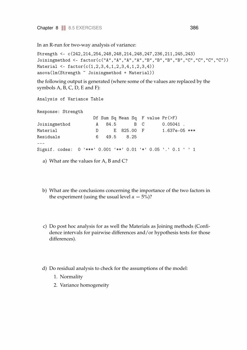
Chapter 8 8.5 EXERCISES 386
In an R-run for two-way analysis of variance:
Strength <- c(242,214,254,248,248,214,248,247,236,211,245,243)Joiningmethod <- factor(c("A","A","A","A","B","B","B","B","C","C","C","C"))Material <- factor(c(1,2,3,4,1,2,3,4,1,2,3,4))anova(lm(Strength ~ Joiningmethod + Material))
the following output is generated (where some of the values are replaced by thesymbols A, B, C, D, E and F):
Analysis of Variance Table
Response: StrengthDf Sum Sq Mean Sq F value Pr(>F)
Joiningmethod A 84.5 B C 0.05041 .Material D E 825.00 F 1.637e-05 ***Residuals 6 49.5 8.25---Signif. codes: 0 '***' 0.001 '**' 0.01 '*' 0.05 '.' 0.1 ' ' 1
a) What are the values for A, B and C?
b) What are the conclusions concerning the importance of the two factors inthe experiment (using the usual level α = 5%)?
c) Do post hoc analysis for as well the Materials as Joining methods (Confi-dence intervals for pairwise differences and/or hypothesis tests for thosedifferences).
d) Do residual analysis to check for the assumptions of the model:
1. Normality
2. Variance homogeneity
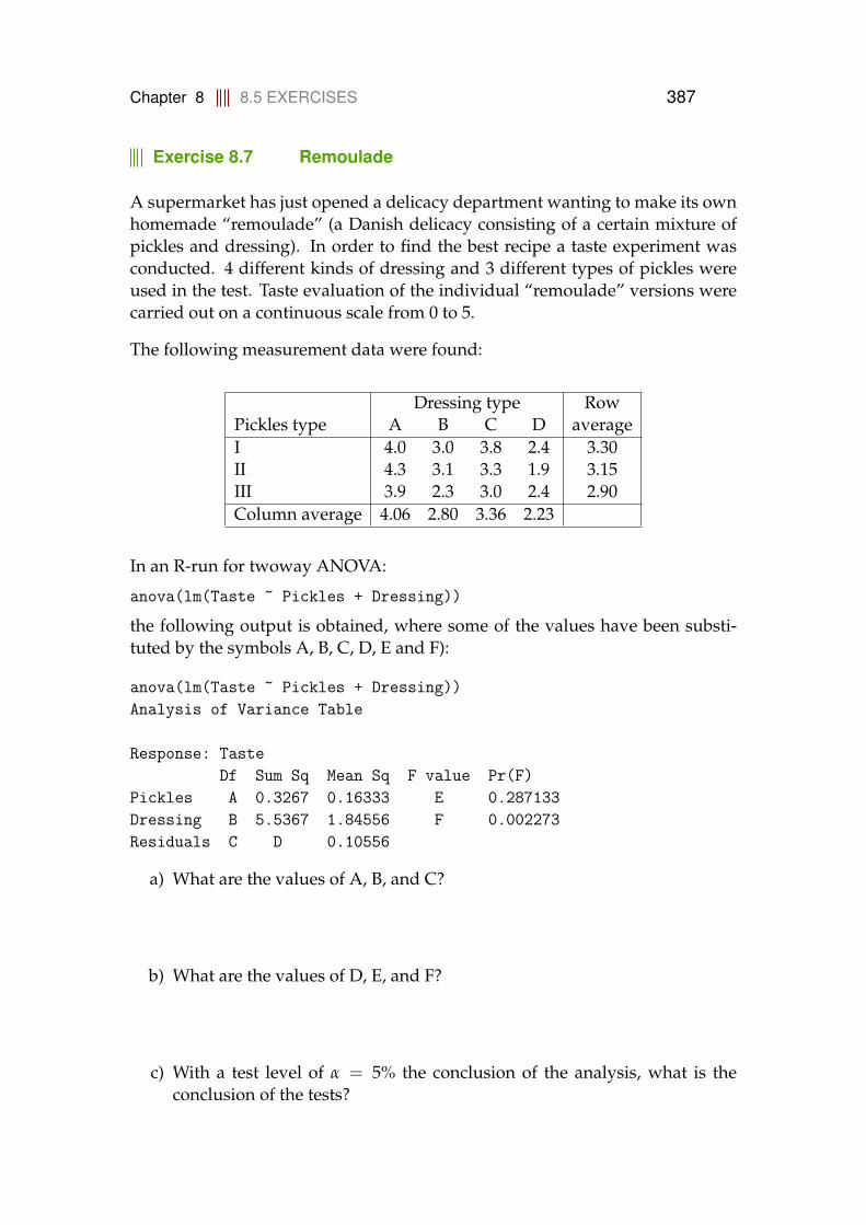
Chapter 8 8.5 EXERCISES 387
Exercise 8.7 Remoulade
A supermarket has just opened a delicacy department wanting to make its ownhomemade “remoulade” (a Danish delicacy consisting of a certain mixture ofpickles and dressing). In order to find the best recipe a taste experiment wasconducted. 4 different kinds of dressing and 3 different types of pickles wereused in the test. Taste evaluation of the individual “remoulade” versions werecarried out on a continuous scale from 0 to 5.
The following measurement data were found:
Dressing type RowPickles type A B C D averageI 4.0 3.0 3.8 2.4 3.30II 4.3 3.1 3.3 1.9 3.15III 3.9 2.3 3.0 2.4 2.90Column average 4.06 2.80 3.36 2.23
In an R-run for twoway ANOVA:
anova(lm(Taste ~ Pickles + Dressing))
the following output is obtained, where some of the values have been substi-tuted by the symbols A, B, C, D, E and F):
anova(lm(Taste ~ Pickles + Dressing))Analysis of Variance Table
Response: TasteDf Sum Sq Mean Sq F value Pr(F)
Pickles A 0.3267 0.16333 E 0.287133Dressing B 5.5367 1.84556 F 0.002273Residuals C D 0.10556
a) What are the values of A, B, and C?
b) What are the values of D, E, and F?
c) With a test level of α = 5% the conclusion of the analysis, what is theconclusion of the tests?
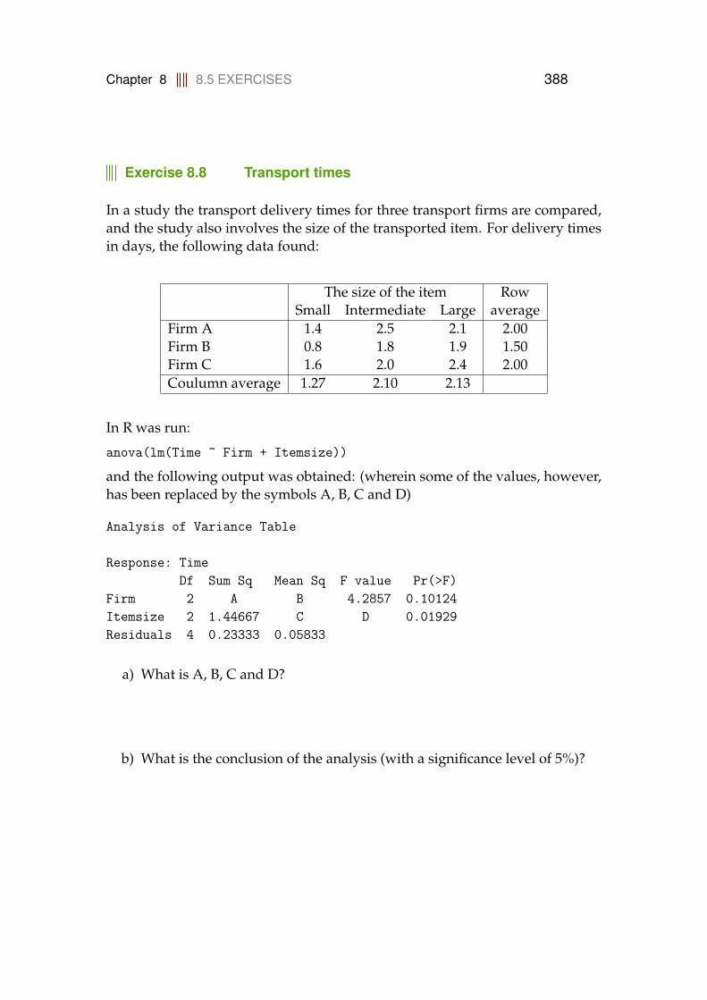
Chapter 8 8.5 EXERCISES 388
Exercise 8.8 Transport times
In a study the transport delivery times for three transport firms are compared,and the study also involves the size of the transported item. For delivery timesin days, the following data found:
The size of the item RowSmall Intermediate Large average
Firm A 1.4 2.5 2.1 2.00Firm B 0.8 1.8 1.9 1.50Firm C 1.6 2.0 2.4 2.00Coulumn average 1.27 2.10 2.13
In R was run:
anova(lm(Time ~ Firm + Itemsize))
and the following output was obtained: (wherein some of the values, however,has been replaced by the symbols A, B, C and D)
Analysis of Variance Table
Response: TimeDf Sum Sq Mean Sq F value Pr(>F)
Firm 2 A B 4.2857 0.10124Itemsize 2 1.44667 C D 0.01929Residuals 4 0.23333 0.05833
a) What is A, B, C and D?
b) What is the conclusion of the analysis (with a significance level of 5%)?
Chapter 8 Glossaries 389
Glossaries
Alternative hypothesis [Alternativ hypotese] The alternative hypothesis (H1)is oftern the negation of the null hypothesis 151
Binomial distribution [Binomial fordeling] If an experiment has two possibleoutcomes (e.g. failure or success, no or yes, 0 or 1) and is repeated morethan one time, then the number of successes is binomial distributed 58
Box plot [Box plot] The so-called boxplot in its basic form depicts the five quar-tiles (min, Q1 , median, Q3 , max) with a box from Q1 to Q3 emphasizingthe Inter Quartile Range (IQR) 29
cumulated distribution function [Fordelingsfunktion]The cdf is the functionwhich determines the probability of observing an outcome of a randomvariable below a given value 396,
χ2-distribution [χ2-fordeling (udtales: chi-i-anden fordeling)] 97, 139
confidence interval [Konfidensinterval] The confidence interval is a way to han-dle the uncertainty by the use of probability theory. The confidence inter-val represents those values of the unknown population mean µ that webelieve is based on the data. Thus we believe the true mean in the statis-tics class is in this interval 130,
Central Limit Theorem [Centrale grænseværdisætning] The Central Limit The-orem (CLT) states that the sample mean of independent identically dis-tributed outcomes converges to a normal distribution 134
Continuous random variable [Kontinuert stokastisk variabel] If an outcome ofan experiment takes a continuous value, for example: a distance, a tem-perature, a weight, etc., then it is represented by a continuous randomvariable 44, 67, 396
Correlation [Korrelation] The sample correlation coefficient are a summary statis-tic that can be calculated for two (related) sets of observations. It quantifies
Chapter 8 Glossaries 390
the (linear) strength of the relation between the two. See also: Covariance16, 88, 395
Covariance [Kovarians] The sample covariance coefficient are a summary statis-tic that can be calculated for two (related) sets of observations. It quantifiesthe (linear) strength of the relation between the two. See also: Correlation16, 88, 395, 397
Critical value Kritisk værdi As an alternative to the p-value one can use the so-called critical values, that is the values of the test-statistic which matchesexactly the significance level 149
Degrees of freedom [Frihedsgrader] The number of "observations" in the datathat are free to vary when estimating statistical parameters often definedas n− 1 97, 176
Descriptive statistics [Beskrivende statistik] Descriptive statistics, or explorativestatistics, is an important part of statistics, where the data is summarizedand described 8
Discrete random variable [Diskret stokastisk variabel] A discrete random vari-able has discrete outcomes and follows a discrete distribution 45
Distribution [Fordeling] Defines how the data is distributed such as, normaldistribution, cumulated distribution function, probability density func-tion exponential distribution, log-normal distribution, Poisson distribu-tion, uniform distribution, hypergeometric distribution, binomial distri-bution, t-distribution, F-distribution 44
Empirical cumulative distribution [Empirisk fordeling] The empirical cumu-lative distribution function Fn is a step function with jumps i/n at obser-vation values, where i is the number of identical observations at that value28
Expectation [Forventningsværdi] A function for calculating the mean. The valuewe expect for a random variable (or function of random variables), henceof the population 53
Exponential distribution [Eksponential fordelingen] The usual application ofthe exponential distribution is for describing the length (usually time) be-tween events which, when counted, follows a Poisson distribution 78
F-distribution [F-fordelingen] The F-distribution appears as the ratio betweentwo independent χ2-distributed random variables 108
Chapter 8 Glossaries 391
Frequency [Frekvens] How frequent data is observed. The frequency distribu-tion of the data for a certain grouping is nicely depicted by the histogram,which is a barplot of either raw frequencies or for some number of classes26
Histogram [Histogram] The default histogram uses the same width for all classesand depicts the raw frequencies/counts in each class. By dividing the rawcounts by n times the class width the density histogram is found wherethe area of all bars sum to 1 26
Hypergeometric distribution [Hypergeometrisk fordeling] 61
Independence [Uafhængighed] 91
Independent samples [Uafhængige stikprøver] 180
(Statistical) Inference [Statistisk inferens (følgeslutninger baseret på data)] 122
Interval [Interval] Data in a specified range 63
Inter Quartile Range [Interkvartil bredde] The Inter Quartile Range (IQR) isthe middle 50% range of data 15, 395
Log-normal distribution [Lognormal fordeling] 78
Maximum likelihood [Estimator baseret på maximum likelihood metoden] 211
Median [Median, stikprøvemedian] The median of population or sample (note,in text no distinguishment between population median and sample median)10, 394
Non-parametric (test) [Ikke-parametriske (tests)] 222
Normal distribution [Normal fordeling] 71
Null hypothesis [Nulhypotese (H0)] 148
One-sample t-test Missing description 153
P-value [p-værdi (for faktisk udfald af en teststørrelse)] 144
probability density function The pdf is the function which determines the prob-ability of every possible outcome of a random variable 396,
Quantile [Fraktil, stikprøvefraktil] The quantiles of population or sample (note,in text no distinguishment between population quantile and sample quantile)11, 394

Chapter 8 Glossaries 392
Quartile [Fraktil, stikprøvefraktil] The quartiles of population or sample (note,in text no distinguishment between population quartile and sample quartile)12, 394
Sample variance [Empirisk varians, stikprøvevarians] 13, 395
Sample mean [Stikprøvegennemsnit] The average of a sample 9, 52, 124, 394
Standard deviation [Standard afvigelse] 395
t-distribution [t-fordeling] 102

Chapter 8 Acronyms 393
Acronyms
ANOVA Analysis of Variance Glossary: Analysis of Variance
cdf cumulated distribution function 46, Glossary: cumulated distribution func-tion
CI confidence interval Glossary: confidence interval
CLT Central Limit Theorem Glossary: Central Limit Theorem
IQR Inter Quartile Range Glossary: Inter Quartile Range
LSD Least Significant Difference Glossary: Least Significant Difference
pdf probability density function Glossary: probability density function

Chapter A 394
Appendix A
Collection of formulas and R commands
This appendix chapter holds a collection of formulas. All the relevant equations from def-initions, methods and theorems are included – along with associated R functions. All arein included in the same order as in the book, except for the distributions which are listedtogether.
A.1 Introduction, descriptive statistics, R and datavisualization
Description Formula R command
1.4 Sample meanThe mean of a sample.
x =1n
n
∑i=1
xi mean(x)
1.5
Sample medianThe value that divides a sam-ple in two halves with equalnumber of observations ineach.
Q2 =
x( n+12 ) for odd n
x( n2 )+x
( n+22 )
2 for even nmedian(x)
1.7
Sample quantileThe value that divide a sam-ple such that p of the obser-vations are less that the value.The 0.5 quantile is the Me-dian.
qp =
{ x(np)+x(np+1)2 for pn integer
x(dnpe) for pn non-integerquantile(x,p,type=2),
1.8
Sample quartilesThe quartiles are the fivequantiles dividing the samplein four parts, such that eachpart holds an equal number ofobservations
Q0 = q0 = “minimum”
Q1 = q0.25 = “lower quartile”
Q2 = q0.5 = “median”
Q3 = q0.75 = “upper quartile”
Q4 = q1 = “maximum”
quantile(x,probs,type=2)
whereprobs=p
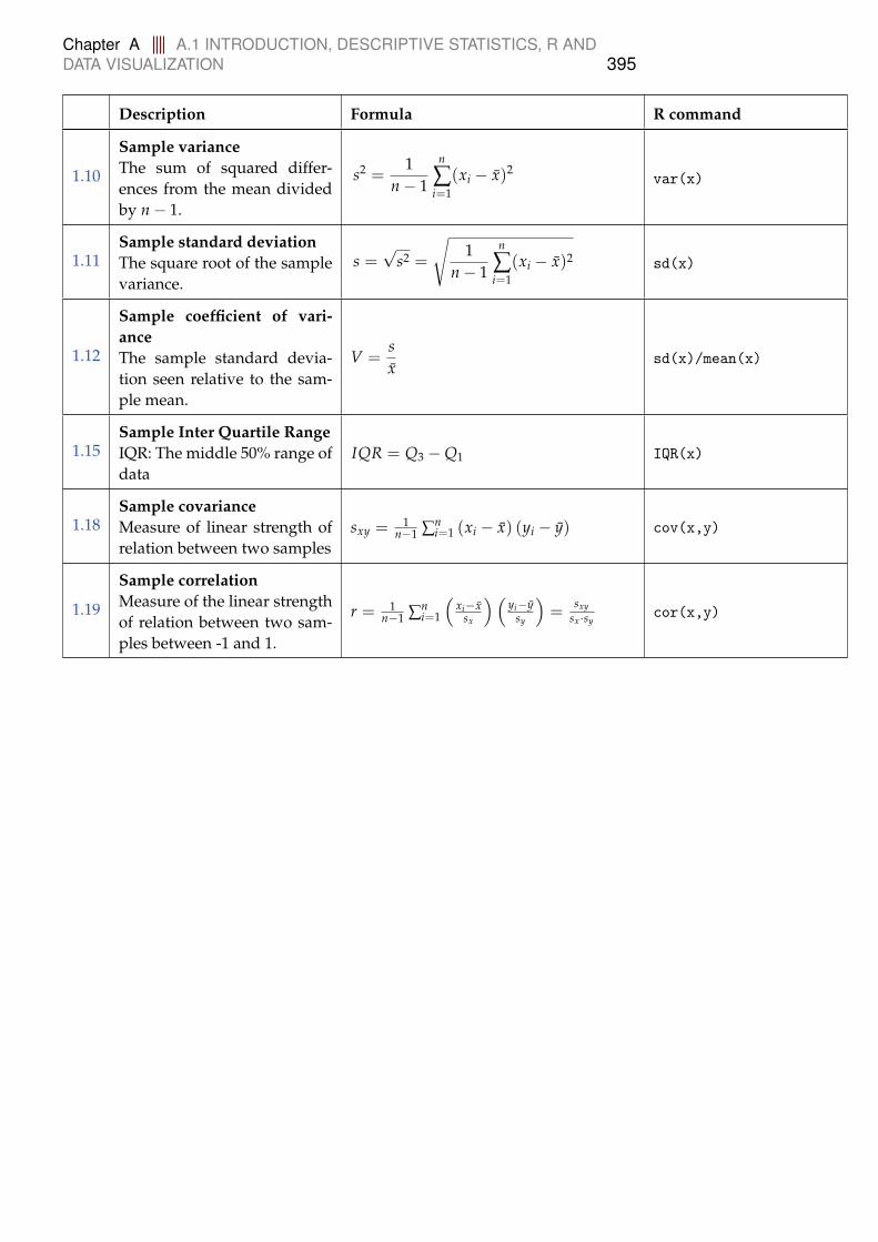
Chapter A A.1 INTRODUCTION, DESCRIPTIVE STATISTICS, R ANDDATA VISUALIZATION 395
Description Formula R command
1.10
Sample varianceThe sum of squared differ-ences from the mean dividedby n− 1.
s2 =1
n− 1
n
∑i=1
(xi − x)2var(x)
1.11Sample standard deviationThe square root of the samplevariance.
s =√
s2 =
√1
n− 1
n
∑i=1
(xi − x)2 sd(x)
1.12
Sample coefficient of vari-anceThe sample standard devia-tion seen relative to the sam-ple mean.
V =sx
sd(x)/mean(x)
1.15Sample Inter Quartile RangeIQR: The middle 50% range ofdata
IQR = Q3 −Q1 IQR(x)
1.18Sample covarianceMeasure of linear strength ofrelation between two samples
sxy = 1n−1 ∑n
i=1 (xi − x) (yi − y) cov(x,y)
1.19
Sample correlationMeasure of the linear strengthof relation between two sam-ples between -1 and 1.
r = 1n−1 ∑n
i=1
(xi−x
sx
) (yi−y
sy
)=
sxysx ·sy
cor(x,y)

Chapter A A.2 PROBABILITY AND SIMULATION 396
A.2 Probability and Simulation
Description Formula R command
2.6
Probability density function(pdf) for a discrete variablefulfills two conditions: f (x) ≥0 and ∑all x f (x) = 1 and findsthe probality for one x value.
f (x) = P(X = x)dnorm,dbinom,dhyper,dpois
2.9
Cumulated distributionfunction (cdf)gives the probability in arange of x values whereP(a < X ≤ b) = F(b)− F(a).
F(x) = P(X ≤ x)pnorm,pbinom,phyper,ppois
2.13Mean of a discrete randomvariable µ = E(X) = ∑∞
i=1 xi f (xi)
2.16Variance of a discrete ran-dom variable X σ2 = Var(X) = E[(X− µ)2]
2.32
Pdf of a continuous randomvariableis a non-negative function forall possible outcomes and hasan area below the function ofone
P(a < X ≤ b) =∫ b
a f (x)dx
2.33
Cdf of a continuous randomvariableis non-decreasingand limx→−∞ F(x) =
0 and limx→∞ F(x) = 1
F(x) = P(X ≤ x) =∫ x−∞ f (u)du
2.34Mean and variance for a con-tinuous random variable X
µ = E(X) =∫ ∞−∞ x f (x)dx
σ2 = E[(X− µ)2] =∫ ∞−∞(x− µ)2 f (x)dx
2.54
Mean and variance of a linearfunctionThe mean and variance of alinear function of a randomvariable X.
E(aX + b) = a E(X) + b
V(aX + b) = a2 V(X)
2.56
Mean and variance of a linearcombinationThe mean and variance of alinear combination of randomvariables.
E(a1X1 + a2X2 + · · ·+ anXn) =
a1 E(X1) + a2 E(X2) + · · ·+ an E(Xn)
V(a1X1 + a2X2 + . . . + anXn) =
a21 V(X1) + a2
2 V(X2) + · · ·+ a2n V(Xn)

Chapter A A.2 PROBABILITY AND SIMULATION 397
Description Formula R command
2.58
CovarianceThe covariance between betwo random variables X andY.
Cov(X, Y) = E [(X− E[X])(Y− E[Y])]
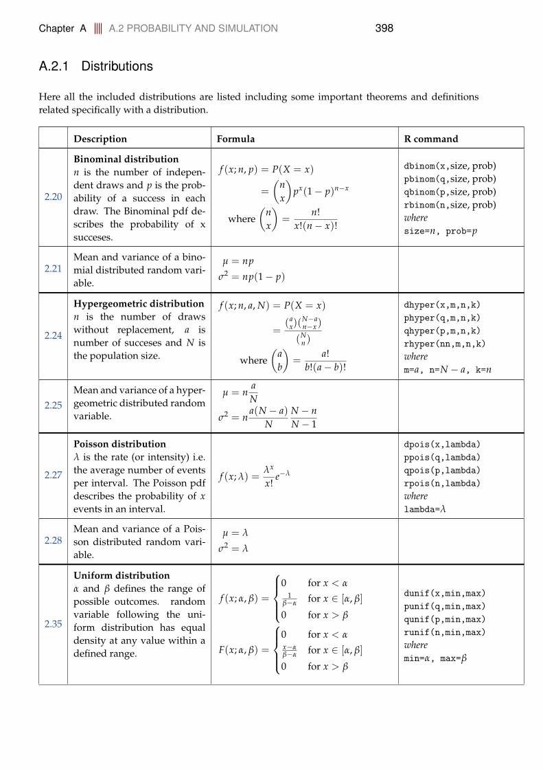
Chapter A A.2 PROBABILITY AND SIMULATION 398
A.2.1 Distributions
Here all the included distributions are listed including some important theorems and definitionsrelated specifically with a distribution.
Description Formula R command
2.20
Binominal distributionn is the number of indepen-dent draws and p is the prob-ability of a success in eachdraw. The Binominal pdf de-scribes the probability of xsucceses.
f (x; n, p) = P(X = x)
=
(nx
)px(1− p)n−x
where(
nx
)=
n!x!(n− x)!
dbinom(x,size, prob)pbinom(q,size, prob)qbinom(p,size, prob)rbinom(n,size, prob)wheresize=n, prob=p
2.21Mean and variance of a bino-mial distributed random vari-able.
µ = np
σ2 = np(1− p)
2.24
Hypergeometric distributionn is the number of drawswithout replacement, a isnumber of succeses and N isthe population size.
f (x; n, a, N) = P(X = x)
=(a
x)(N−an−x)
(Nn )
where(
ab
)=
a!b!(a− b)!
dhyper(x,m,n,k)phyper(q,m,n,k)qhyper(p,m,n,k)rhyper(nn,m,n,k)wherem=a, n=N − a, k=n
2.25Mean and variance of a hyper-geometric distributed randomvariable.
µ = naN
σ2 = na(N − a)
NN − nN − 1
2.27
Poisson distributionλ is the rate (or intensity) i.e.the average number of eventsper interval. The Poisson pdfdescribes the probability of xevents in an interval.
f (x; λ) =λx
x!e−λ
dpois(x,lambda)ppois(q,lambda)qpois(p,lambda)rpois(n,lambda)wherelambda=λ
2.28Mean and variance of a Pois-son distributed random vari-able.
µ = λ
σ2 = λ
2.35
Uniform distributionα and β defines the range ofpossible outcomes. randomvariable following the uni-form distribution has equaldensity at any value within adefined range.
f (x; α, β) =
0 for x < α1
β−α for x ∈ [α, β]
0 for x > β
F(x; α, β) =
0 for x < αx−αβ−α for x ∈ [α, β]
0 for x > β
dunif(x,min,max)punif(q,min,max)qunif(p,min,max)runif(n,min,max)wheremin=α, max=β
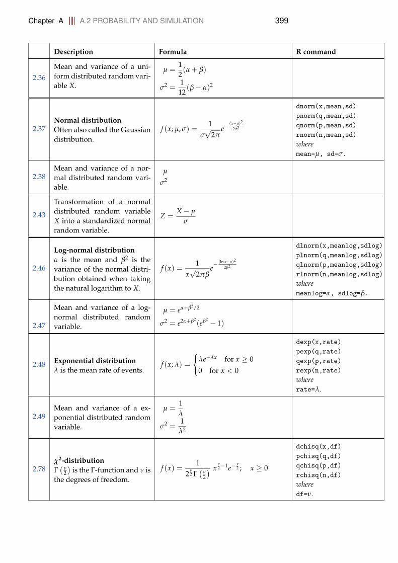
Chapter A A.2 PROBABILITY AND SIMULATION 399
Description Formula R command
2.36Mean and variance of a uni-form distributed random vari-able X.
µ =12(α + β)
σ2 =1
12(β− α)2
2.37Normal distributionOften also called the Gaussiandistribution.
f (x; µ, σ) =1
σ√
2πe−
(x−µ)2
2σ2
dnorm(x,mean,sd)pnorm(q,mean,sd)qnorm(p,mean,sd)rnorm(n,mean,sd)wheremean=µ, sd=σ.
2.38Mean and variance of a nor-mal distributed random vari-able.
µ
σ2
2.43
Transformation of a normaldistributed random variableX into a standardized normalrandom variable.
Z =X− µ
σ
2.46
Log-normal distributionα is the mean and β2 is thevariance of the normal distri-bution obtained when takingthe natural logarithm to X.
f (x) =1
x√
2πβe− (ln x−α)2
2β2
dlnorm(x,meanlog,sdlog)plnorm(q,meanlog,sdlog)qlnorm(p,meanlog,sdlog)rlnorm(n,meanlog,sdlog)wheremeanlog=α, sdlog=β.
2.47
Mean and variance of a log-normal distributed randomvariable.
µ = eα+β2/2
σ2 = e2α+β2(eβ2 − 1)
2.48 Exponential distributionλ is the mean rate of events.
f (x; λ) =
{λe−λx for x ≥ 0
0 for x < 0
dexp(x,rate)pexp(q,rate)qexp(p,rate)rexp(n,rate)whererate=λ.
2.49Mean and variance of a ex-ponential distributed randomvariable.
µ =1λ
σ2 =1
λ2
2.78χ2-distributionΓ(
ν2
)is the Γ-function and ν is
the degrees of freedom.
f (x) =1
2ν2 Γ(
ν2
) xν2−1e−
x2 ; x ≥ 0
dchisq(x,df)pchisq(q,df)qchisq(p,df)rchisq(n,df)wheredf=ν.
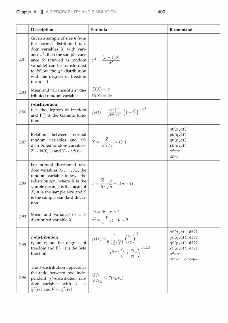
Chapter A A.2 PROBABILITY AND SIMULATION 400
Description Formula R command
2.81
Given a sample of size n fromthe normal distributed ran-dom variables Xi with vari-ance σ2, then the sample vari-ance S2 (viewed as randomvariable) can be transformedto follow the χ2 distributionwith the degrees of freedomν = n− 1.
χ2 =(n− 1)S2
σ2
2.83 Mean and variance of a χ2 dis-tributed random variable.
E(X) = ν
V(X) = 2ν
2.86
t-distributionν is the degrees of freedomand Γ() is the Gamma func-tion.
fT(t) =Γ( ν+1
2 )√νπ Γ( ν
2 )
(1 + t2
ν
)− ν+12
2.87
Relation between normalrandom variables and χ2-distributed random variables.Z ∼ N(0, 1) and Y ∼ χ2(ν).
X =Z√Y/ν
∼ t(ν)
dt(x,df)pt(q,df)qt(p,df)rt(n,df)wheredf=ν.
2.89
For normal distributed ran-dom variables X1, . . . , Xn, therandom variable follows thet-distribution, where X is thesample mean, µ is the mean ofX, n is the sample size and Sis the sample standard devia-tion.
T =X− µ
S/√
n∼ t(n− 1)
2.93 Mean and variance of a t-distributed variable X.
µ = 0; ν > 1
σ2 =ν
ν− 2; ν > 2
2.95
F-distributionν1 an ν2 are the degrees offreedom and B(·, ·) is the Betafunction.
fF(x) =1
B( ν1
2 , ν22
)(
ν1
ν2
) ν12
· xν12 −1
(1 +
ν1
ν2x)− ν1+ν2
2
df(x,df1,df2)pf(q,df1,df2)qf(p,df1,df2)rf(n,df1,df2)wheredf1=ν1,df2=µ2.
2.96
The F-distribution appears asthe ratio between two inde-pendent χ2-distributed ran-dom variables with U ∼χ2(ν1) and V ∼ χ2(ν2).
U/ν1
V/ν2∼ F(ν1, ν2)

Chapter A A.2 PROBABILITY AND SIMULATION 401
Description Formula R command
2.98
X1, . . . , Xn1 and Y1, . . . , Yn2
with the mean µ1 and µ2
and the variance σ21 and σ2
2is independent and sampledfrom a normal distribution.
S21/σ2
1
S22/σ2
2∼ F(n1 − 1, n2 − 1)
2.101 Mean and variance of a F-distributed variable X.
µ =ν2
ν2 − 2; ν2 > 2
σ =2ν2
2(ν1 + ν2 − 2)ν1(ν2 − 2)2(ν2 − 4)
; ν2 > 4
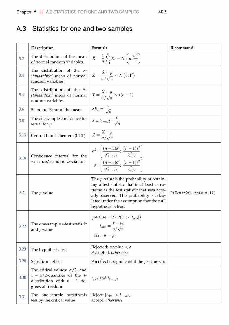
Chapter A A.3 STATISTICS FOR ONE AND TWO SAMPLES 402
A.3 Statistics for one and two samples
Description Formula R command
3.2 The distribution of the meanof normal random variables.
X =1n
n
∑i=1
Xi ∼ N(
µ,σ2
n
)
3.4The distribution of the σ-standardized mean of normalrandom variables
Z =X− µ
σ/√
n∼ N
(0, 12)
3.4The distribution of the S-standardized mean of normalrandom variables
T =X− µ
S/√
n∼ t(n− 1)
3.6 Standard Error of the mean SEx =s√n
3.8 The one sample confidence in-terval for µ
x± t1−α/2 ·s√n
3.13 Central Limit Theorem (CLT) Z =X− µ
σ/√
n
3.18 Confidence interval for thevariance/standard deviation
σ2 :
[(n− 1)s2
χ21−α/2
;(n− 1)s2
χ2α/2
]
σ :
[(n− 1)s2
χ21−α/2
;(n− 1)s2
χ2α/2
]
3.21 The p-value
The p-valueis the probability of obtain-ing a test statistic that is at least as ex-treme as the test statistic that was actu-ally observed. This probability is calcu-lated under the assumption that the nullhypothesis is true.
P(T>x)=2(1-pt(x,n-1))
3.22 The one-sample t-test statisticand p-value
p-value = 2 · P(T > |tobs|)
tobs =x− µ0
s/√
nH0 : µ = µ0
3.23 The hypothesis testRejected: p-value < α
Accepted: otherwise
3.28 Significant effect An effect is significant if the p-value< α
3.30
The critical values: α/2- and1 − α/2-quantiles of the t-distribution with n − 1 de-grees of freedom
tα/2 and t1−α/2
3.31 The one-sample hypothesistest by the critical value
Reject: |tobs| > t1−α/2accept: otherwise
Chapter A A.3 STATISTICS FOR ONE AND TWO SAMPLES 403
Description Formula R command
3.32 Confidence interval for µx± t1−α/2 · s√
nacceptance region/CI: H0 : µ = µ0
3.35 The level α one-sample t-test
Test: H0 : µ = µ0 and H1 : µ 6= µ0 byp-value = 2 · P(T > |tobs|)Reject: p-value < α or |tobs| > t1−α/2Accept: Otherwise
3.62The one-sample confidenceinterval (CI) sample size for-mula
n =( z1−α/2·σ
ME
)2
3.64 The one-sample sample sizeformula
n =(
σz1−β+z1−α/2(µ0−µ1)
)2
3.41 The Normal q-q plot withn > 10
naive approach: pi =in , i = 1, . . . , n
commonly aproach: pi = i−0.5n+1 , i =
1, . . . , n
3.48 The (Welch) two-sample t-teststatistic
δ = µ2 − µ1
H0 : δ = δ0
tobs =(x1−x2)−δ0√s2
1/n1+s22/n2
3.49 The distribution of the(Welch) two-sample statistic
T = (X1−X2)−δ0√S2
1/n1+S22/n2
ν =
(s21
n1+
s22
n2
)2
(s21/n1)
2
n1−1 +(s2
2/n2)2
n2−1
3.50 The level α two-sample t-test
Test: H0 : µ1 − µ2 = δ0 and H1 : µ1 −µ2 6= δ0 by p-value = 2 · P(T > |tobs|)Reject: p-value < α or |tobs| > t1−α/2Accept: Otherwise
3.51 The pooled two-sample esti-mate of variance
s2p =
(n1−1)s21+(n2−1)s2
2n1+n2−2
3.52 The pooled two-sample t-teststatistic
δ = µ1 − µ2
H0 : δ = δ0
tobs =(x1−x2)−δ0√s2
p/n1+s2p/n2
3.53 The distribution of the pooledtwo-sample t-test statistic
T = (X1−X2)−δ0√S2
p/n1+S2p/n2
3.46 The two-sample confidenceinterval for µ1 − µ2
x− y± t1−α/2 ·√
s21
n1+
s22
n2
ν =
(s21
n1+
s22
n2
)2
(s21/n1)
2
n1−1 +(s2
2/n2)2
n2−1
Chapter A A.4 SIMULATION BASED STATISTICS 404
A.4 Simulation based statistics
Description Formula R command
4.3 The non-linear approximativeerror propagation rule
σ2f (X1,...,Xn)
= ∑ni=1
(∂ f∂xi
)2σ2
i
4.4 Non-linear error propagationby simulation
1. Simulate k outcomes2. Calculate the standard deviation by
ssimf (X1,...,Xn)
=√
1k−1 ∑k
i=1( f j − f )2
4.7Confidence interval for anyfeature θ by parametric boot-strap
1.Simulate k samples2.Calculate the statistic θ
3.Calculate CI:[q∗100(α/2)%, q∗100(1−α/2)%
]
4.10
Two-sample confidence inter-val for any feature compar-ison θ1 − θ2 by parametricbootstrap
1.Simulate k sets of 2 samples2.Calculate the statistic θ∗xk − θ∗yk
3.Calculate CI:[q∗100(α/2)%, q∗100(1−α/2)%
]
Chapter A A.5 SIMPLE LINEAR REGRESSION 405
A.5 Simple linear regression
Description Formula R command
5.4 Least square estimators
β1 =∑n
i=1(Yi − Y)(xi − x)Sxx
β0 = Y− β1 x
where Sxx = ∑ni=1(xi − x)2
5.7 Variance of estimators
V[β0] =σ2
n+
x2σ2
Sxx
V[β1] =σ2
Sxx
Cov[β0, β1] = −xσ2
Sxx
5.11 Tests statistics for H0 : β0 = 0and H0 : β1 = 0
Tβ0 =β0 − β0,0
σβ0
Tβ1 =β1 − β0,1
σβ1
5.13 Level α t-tests for parameter
Test H0,i : βi = β0,i vs. H1,i : βi 6= β0,iwith p-value = 2 · P(T > |tobs,βi |)where tobs,βi =
βi−β0,iσβi
.If p-value < α then reject H0,otherwise accept H0
D <- data.frame(x=c(), y=c())
fit <- lm(y~x, data=D)summary(fit)
5.14 Parameter confidence inter-vals
β0 ± t1−α/2 σβ0
β1 ± t1−α/2 σβ1
confint(fit,level=0.95)
5.17 Confident and prediction in-terval
Confidence interval for the line:
β0 + β1xnew ± t1−α/2σ√
1n + (xnew−x)2
Sxx
Interval for a new point prediction:
β0 + β1xnew ± t1−α/2σ√
1 + 1n + (xnew−x)2
Sxx
predict(fit,newdata=data.frame(),interval="confidence",level=0.95)
predict(fit,newdata=data.frame(),interval="prediction",level=0.95)
5.21
The matrix formulation ofthe parameter estimators inthe simple linear regressionmodel
β = (XTX)−1XTY
V[β] = σ2(XTX)−1
σ2 =RSS
n− 2
5.23
Coefficient of determinationR2 r2 = 1− ∑i(yi−yi)
2
∑i(yi−y)2

Chapter A A.5 SIMPLE LINEAR REGRESSION 406
Description Formula R command
5.7 Model validation of assump-tions
> Check the normality assumption witha q-q plot of the residuals.
> Check the systematic behavior byplotting the residuals ei as a function offitted values yi
qqnorm(fit$residuals)qqline(fit$residuals)
plot(fit$fitted.values,fit$residuals)

Chapter A A.6 MULTIPLE LINEAR REGRESSION 407
A.6 Multiple linear regression
Description Formula R command
6.2 Level α t-tests for parameter
Test H0,i : βi = β0,i vs. H1,i : βi 6= β0,iwith p-value = 2 · P(T > |tobs,βi |)where tobs,βi =
βi−β0,iσβi
.If p-value < α the reject H0,otherwise accept H0
D<-data.frame(x1=c(),x2=c(),y=c())
fit <- lm(y~x1+x2,data=D)
summary(fit)
6.5 Parameter confidence inter-vals
βi ± t1−α/2 σβi confint(fit,level=0.95)
6.9 Confident and prediction in-terval (in R)
Confident interval for the lineβ0 + β1x1,new + · · ·+ βpxp,new
Interval for a new point predictionβ0 + β1x1,new + · · ·+ βpxp,new + εnew
predict(fit,newdata=data.frame(),interval="confidence",level=0.95)
predict(fit,newdata=data.frame(),interval="prediction",level=0.95)
6.17
The matrix formulation ofthe parameter estimators inthe multiple linear regressionmodel
β = (XTX)−1XTY
V[β] = σ2(XTX)−1
σ2 =RSS
n− (p + 1)
6.16 Model selection procedureBackward selection: start with fullmodel and stepwise remove insignifi-cant terms
Chapter A A.7 INFERENCE FOR PROPORTIONS 408
A.7 Inference for proportions
Description Formula R command
7.3 Proportion estimate and con-fidence interval
p = xn
p± z1−α/2
√p(1− p)
n
prop.test(x=, n=,correct=FALSE)
7.10 Approximate proportion withZ
Z = X−np0√np0(1−p0)
∼ N(0, 1)
7.11 The level α one-sample pro-portion hypothesis test
Test: H0 : p = p0, vs. H1 : p 6= p0
by p-value = 2 · P(Z > |zobs|)where Z ∼ N(0, 12)
If p-value < α the reject H0,otherwise accept H0
prop.test(x=, n=,correct=FALSE)
7.13 Sample size formula for the CIof a proportion
Guessed p (with prior knowledge):n = p(1− p)( z1−α/2
ME )2
Unknown p:n = 1
4 (z1−α/2
ME )2
7.15
Difference of two proportionsestimator p1 − p2 and confi-dence interval for the differ-ence
σp1− p2 =√
p1(1− p1)n1
+ p2(1− p2)n2
( p1 − p2)± z1−α/2 · σp1− p2
7.18 The level α one-sample t-test
Test: H0 : p1 = p2, vs. H1 : p1 6= p2
by p-value = 2 · P(Z > |zobs|)where Z ∼ N(0, 12)
If p-value < α the reject H0,otherwise accept H0
prop.test(x=, n=,correct=FALSE)
7.20 The multi-sample proportionsχ2-test
Test: H0 : p1 = p2 = . . . = pc = p
by χ2obs = ∑2
i=1 ∑cj=1
(oij−eij)2
eij
chisq.test(X,correct = FALSE)
7.22 The r × c frequency table χ2-test
Test: H0 : pi1 = pi2 = . . . = pic = pifor all rows i = 1, 2, . . . , rby χ2
obs = ∑ri=1 ∑c
j=1(oij−eij)
2
eij
Reject if χ2obs > χ2
1−α
((r− 1)(c− 1)
)
Otherwise accept
chisq.test(X,correct = FALSE)
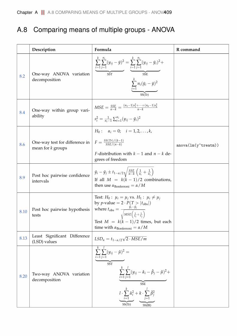
Chapter A A.8 COMPARING MEANS OF MULTIPLE GROUPS - ANOVA409
A.8 Comparing means of multiple groups - ANOVA
Description Formula R command
8.2 One-way ANOVA variationdecomposition
k
∑i=1
ni
∑j=1
(yij − y)2
︸ ︷︷ ︸SST
=k
∑i=1
ni
∑j=1
(yij − yi)2
︸ ︷︷ ︸SSE
+
k
∑i=1
ni(yi − y)2
︸ ︷︷ ︸SS(Tr)
8.4 One-way within group vari-ability
MSE = SSEn−k =
(n1−1)s21+···+(nk−1)s2
kn−k
s2i = 1
ni−1 ∑nii=1(yij − yi)
2
8.6 One-way test for difference inmean for k groups
H0 : αi = 0; i = 1, 2, . . . , k,
F = SS(Tr)/(k−1)SSE/(n−k)
F-distribution with k − 1 and n − k de-grees of freedom
anova(lm(y~treatm))
8.9 Post hoc pairwise confidenceintervals
yi − yj ± t1−α/2
√SSEn−k
(1ni+ 1
nj
)
If all M = k(k − 1)/2 combinations,then use αBonferroni = α/M
8.10 Post hoc pairwise hypothesistests
Test: H0 : µi = µj vs. H1 : µi 6= µjby p-value = 2 · P(T > |tobs|)where tobs =
yi−yj√MSE
(1ni+ 1
nj
)
Test M = k(k − 1)/2 times, but eachtime with αBonferroni = α/M
8.13 Least Significant Difference(LSD) values
LSDα = t1−α/2√
2 ·MSE/m
8.20 Two-way ANOVA variationdecomposition
k
∑i=1
l
∑j=1
(yij − µ)2
︸ ︷︷ ︸SST
=
k
∑i=1
l
∑j=1
(yij − αi − β j − µ)2
︸ ︷︷ ︸SSE
+
l ·k
∑i=1
α2i
︸ ︷︷ ︸SS(Tr)
+ k ·l
∑j=1
β2j
︸ ︷︷ ︸SS(Bl)

Chapter A A.8 COMPARING MEANS OF MULTIPLE GROUPS - ANOVA410
Description Formula R command
8.22Test for difference in means intwo-way ANOVA grouped intreatments and in blocks
H0,Tr : αi = 0, i = 1, 2, . . . , k
FTr =SS(Tr)/(k− 1)
SSE/((k− 1)(l − 1))
H0,Bl : β j = 0, j = 1, 2, . . . , l
FBl =SS(Bl)/(l − 1)
SSE/((k− 1)(l − 1))
fit<-lm(y~treatm+block)anova(fit)
One-way ANOVA
Source of Degrees of Sums of Mean sum of Test- p-
variation freedom squares squares statistic F value
Treatment k− 1 SS(Tr) MS(Tr) = SS(Tr)k−1 Fobs =
MS(Tr)MSE P(F > Fobs)
Residual n− k SSE MSE = SSEn−k
Total n− 1 SST
Two-way ANOVA
Source of Degrees of Sums of Mean sums of Test p-
variation freedom squares squares statistic F value
Treatment k− 1 SS(Tr) MS(Tr) = SS(Tr)k−1 FTr =
MS(Tr)MSE P(F > FTr)
Block l − 1 SS(Bl) MS(Bl) = SS(Bl)l−1 FBl =
MS(Bl)MSE P(F > FBl)
Residual (l − 1)(k− 1) SSE MSE = SSE(k−1)(l−1)
Total n− 1 SST