integrals involving and 653 2.1. Constraints on the...
109
Annals of Mathematics 174 (2011), 647–755 http://dx.doi.org/10.4007/annals.2011.174.2.1 Rearrangement inequalities and applications to isoperimetric problems for eigenvalues By Franc ¸ois Hamel, Nikolai Nadirashvili, and Emmanuel Russ Abstract Let Ω be a bounded C 2 domain in R n , where n is any positive inte- ger, and let Ω * be the Euclidean ball centered at 0 and having the same Lebesgue measure as Ω. Consider the operator L = -div(A∇)+ v ·∇ + V on Ω with Dirichlet boundary condition, where the symmetric matrix field A is in W 1,∞ (Ω), the vector field v is in L ∞ (Ω, R n ) and V is a continu- ous function in Ω. We prove that minimizing the principal eigenvalue of L when the Lebesgue measure of Ω is fixed and when A, v and V vary under some constraints is the same as minimizing the principal eigenvalue of some operators L * in the ball Ω * with smooth and radially symmetric coefficients. The constraints which are satisfied by the original coefficients in Ω and the new ones in Ω * are expressed in terms of some distribution functions or some integral, pointwise or geometric quantities. Some strict comparisons are also established when Ω is not a ball. To these purposes, we associate to the principal eigenfunction ϕ of L a new symmetric re- arrangement defined on Ω * , which is different from the classical Schwarz symmetrization and which preserves the integral of div(A∇ϕ) on suitable equi-measurable sets. A substantial part of the paper is devoted to the proofs of pointwise and integral inequalities of independent interest which are satisfied by this rearrangement. The comparisons for the eigenvalues hold for general operators of the type L and they are new even for sym- metric operators. Furthermore they generalize, in particular, and provide an alternative proof of the well-known Rayleigh-Faber-Krahn isoperimetric inequality about the principal eigenvalue of the Laplacian under Dirichlet boundary condition on a domain with fixed Lebesgue measure. Contents 1. Introduction 648 2. Main results 651 2.1. Constraints on the distribution function of V - and on some integrals involving Λ and v 653 647
Transcript of integrals involving and 653 2.1. Constraints on the...
Annals of Mathematics 174 (2011), 647–755http://dx.doi.org/10.4007/annals.2011.174.2.1
Rearrangement inequalities andapplications to isoperimetric problems
for eigenvalues
By Francois Hamel, Nikolai Nadirashvili, and Emmanuel Russ
Abstract
Let Ω be a bounded C2 domain in Rn, where n is any positive inte-
ger, and let Ω∗ be the Euclidean ball centered at 0 and having the same
Lebesgue measure as Ω. Consider the operator L = −div(A∇) + v · ∇+ V
on Ω with Dirichlet boundary condition, where the symmetric matrix field
A is in W 1,∞(Ω), the vector field v is in L∞(Ω,Rn) and V is a continu-
ous function in Ω. We prove that minimizing the principal eigenvalue of
L when the Lebesgue measure of Ω is fixed and when A, v and V vary
under some constraints is the same as minimizing the principal eigenvalue
of some operators L∗ in the ball Ω∗ with smooth and radially symmetric
coefficients. The constraints which are satisfied by the original coefficients
in Ω and the new ones in Ω∗ are expressed in terms of some distribution
functions or some integral, pointwise or geometric quantities. Some strict
comparisons are also established when Ω is not a ball. To these purposes,
we associate to the principal eigenfunction ϕ of L a new symmetric re-
arrangement defined on Ω∗, which is different from the classical Schwarz
symmetrization and which preserves the integral of div(A∇ϕ) on suitable
equi-measurable sets. A substantial part of the paper is devoted to the
proofs of pointwise and integral inequalities of independent interest which
are satisfied by this rearrangement. The comparisons for the eigenvalues
hold for general operators of the type L and they are new even for sym-
metric operators. Furthermore they generalize, in particular, and provide
an alternative proof of the well-known Rayleigh-Faber-Krahn isoperimetric
inequality about the principal eigenvalue of the Laplacian under Dirichlet
boundary condition on a domain with fixed Lebesgue measure.
Contents
1. Introduction 648
2. Main results 651
2.1. Constraints on the distribution function of V − and on some
integrals involving Λ and v 653
647
648 F. HAMEL, N. NADIRASHVILI, and E. RUSS
2.2. Constraints on the determinant and another symmetric function
of the eigenvalues of A 656
2.3. Faber-Krahn inequalities for nonsymmetric operators 659
2.4. Some comparisons with results in the literature 661
2.5. Main tools: a new type of symmetrization 664
3. Inequalities for the rearranged functions 666
3.1. General framework, definitions of the rearrangements and basic
properties 666
3.2. Pointwise comparison between ψ and ψ 673
3.3. A pointwise differential inequality for the rearranged data 677
3.4. An integral inequality for the rearranged data 680
4. Improved inequalities when Ω is not a ball 684
5. Application to eigenvalue problems 691
5.1. Approximation of symmetrized fields by fields having given
distribution functions 692
5.2. Operators whose coefficients have given averages or given
distribution functions 694
5.3. Constraints on the eigenvalues of the matrix field A 727
6. The cases of Lp constraints 730
6.1. Optimization in fixed domains 730
6.2. Faber-Krahn inequalities 739
7. Appendix 742
7.1. Proof of the approximation Lemma 5.1 742
7.2. A remark on distribution functions 747
7.3. Estimates of λ1(BnR, τer) as τ → +∞ 748
References 752
1. Introduction
Throughout all the paper, we fix an integer n ≥ 1 and denote by αn =
πn/2/Γ(n/2 + 1) the Lebesgue measure of the Euclidean unit ball in Rn. By
“domain”, we mean a nonempty open connected subset of Rn, and we denote
by C the set of all bounded domains of Rn which are of class C2. Throughout
all the paper, unless otherwise specified, Ω will always be in the class C. For
any measurable subset A ⊂ Rn, |A| stands for the Lebesgue measure of A. If
Ω ∈ C, then Ω∗ will denote the Euclidean ball centered at 0 such that
|Ω∗| = |Ω| .
Define also C(Ω) (resp. C(Ω,Rn)) the space of real-valued (resp. Rn-valued)
continuous functions on Ω. For all x ∈ Rn \ 0, set
(1.1) er(x) =x
|x|,
REARRANGEMENT INEQUALITIES 649
where |x| denotes the Euclidean norm of x. Finally, if Ω ∈ C, if v : Ω→ Rn is
measurable and if 1 ≤ p ≤ +∞, we say that v ∈ Lp(Ω,Rn) if |v| ∈ Lp(Ω), and
write (somewhat abusively) ‖v‖p or ‖v‖Lp(Ω,Rn) instead of ‖|v|‖Lp(Ω,R).
Various rearrangement techniques for functions defined on Ω were consid-
ered in the literature. The most famous one is the Schwarz symmetrization.
Let us briefly recall what the idea of this symmetrization is. For any function
u ∈ L1(Ω), denote by µu the distribution function of u, given by
µu(t) = |x ∈ Ω; u(x) > t|
for all t ∈ R. Note that µ is right-continuous, nonincreasing and µu(t) → 0
(resp. µu(t)→ |Ω|) as t→ +∞ (resp. t→ −∞). For all x ∈ Ω∗\0, define
u∗(x) = sup t ∈ R; µu(t) ≥ αn |x|n .
The function u∗ is clearly radially symmetric, nonincreasing in the variable |x|,and it satisfies
|x ∈ Ω, u(x) > ζ| = |x ∈ Ω∗, u∗(x) > ζ|
for all ζ ∈ R. An essential property of the Schwarz symmetrization is the
following one: if u ∈ H10 (Ω), then |u|∗ ∈ H1
0 (Ω∗) and (see [41])
(1.2) ‖ |u|∗‖L2(Ω∗) = ‖u‖L2(Ω) and ‖∇|u|∗‖L2(Ω∗) ≤ ‖∇u‖L2(Ω) .
One of the main applications of this rearrangement technique is the resolu-
tion of optimization problems for the eigenvalues of some second-order elliptic
operators on Ω. Let us briefly recall some of these problems. If λ1(Ω) de-
notes the first eigenvalue of the Laplace operator in Ω with Dirichlet boundary
condition, then it is well known that λ1(Ω) ≥ λ1(Ω∗) and that the inequality
is strict unless Ω is a ball (remember that Ω is always assumed to be in the
class C). Since λ1(Ω∗) can be explicitly computed, this result provides the
classical Rayleigh-Faber-Krahn inequality, which states that
(1.3) λ1(Ω) ≥ λ1(Ω∗) =
Ç1
|Ω|
å2/n
α2/nn (jn/2−1,1)2,
where jm,1 the first positive zero of the Bessel function Jm. Moreover, equality
in (1.3) is attained if and only if Ω is a ball. This result was first conjectured
by Rayleigh for n = 2 ([42, pp. 339–340]), and proved independently by Faber
([21]) and Krahn ([30]) for n = 2, and by Krahn for all n in [31] (see [33] for
the English translation). The proof of the inequality λ1(Ω) ≥ λ1(Ω∗) is an
immediate consequence of the following variational formula for λ1(Ω):
(1.4) λ1(Ω) = minv∈H1
0 (Ω)\0
∫Ω|∇v(x)|2 dx∫
Ω|v(x)|2 dx
and of the properties (1.2) of the Schwarz symmetrization.
650 F. HAMEL, N. NADIRASHVILI, and E. RUSS
Lots of optimization results involving other eigenvalues of the Laplacian
(or more general elliptic symmetric operators of the form −div(A∇)) on Ω
under Dirichlet boundary condition have also been established. For instance,
the minimum of λ2(Ω) (the second eigenvalue of the Laplace operator in Ω un-
der Dirichlet boundary condition) among bounded open sets of Rn with given
Lebesgue measure is achieved by the union of two identical balls (this result
is attributed to Szego; see [39]). Very few things seem to be known about
optimization problems for the other eigenvalues; see [17], [25], [39], [40], and
[49]. Various optimization results are also known for functions of the eigenval-
ues. For instance, it is proved in [5] that λ2(Ω)/λ1(Ω) ≤ λ2(Ω∗)/λ1(Ω∗), and
the equality is attained if and only if Ω is a ball. The same result was also
extended in [5] to elliptic operators in divergence form with definite weight.
We also refer to [6], [7], [9], [12], [18], [28], [29], [32], [34], [37], [38], and [40]
for further bounds or other optimization results for some eigenvalues or some
functions of the eigenvalues in fixed or varying domains of Rn (or of manifolds).
Other boundary conditions may also be considered. For instance, if µ2(Ω)
is the first nontrivial eigenvalue of −∆ under the Neumann boundary condi-
tion, then µ2(Ω) ≤ µ2(Ω∗) and the equality is attained if, and only if, Ω is a ball
(see [44] in dimension n = 2, and [48] in any dimension). Bounds or optimiza-
tion results for other eigenvalues of the Laplacian under Neumann boundary
condition ([40], [44], [48]; see also [10] for inhomogeneous problems), for Robin
boundary condition ([15], [19], [20]) or for the Stekloff eigenvalue problem ([16])
have also been established. We also mention another Rayleigh conjecture for
the lowest eigenvalue of the clamped plate. If Ω ⊂ R2, then denote by Λ1(Ω)
the lowest eigenvalue of the operator ∆2, so that ∆2u1 = Λ1(Ω)u1 in Ω with
u1 = ν · ∇u1 = 0 on ∂Ω, where u1 denotes the principal eigenfunction and
ν denotes the outward unit normal on ∂Ω. The second author proved in [35]
that Λ1(Ω) ≥ Λ1(Ω∗) and that equality holds if and only if Ω is a ball, that is
a disk in dimension n = 2. The analogous result was also established in R3 in
[8], while the problem is still open in higher dimensions. Much more complete
surveys of all these topics can be found in [11], [25], and [26].
It is important to observe that the variational formula (1.4) relies heavily
on the fact that −∆ is symmetric on L2(Ω). More generally, all the opti-
mization problems considered hitherto concern symmetric operators, and their
resolution relies on a “Rayleigh” quotient (that is, a variational formula similar
to (1.4)) and the Schwarz symmetrization. Before going further, let us recall
that rearrangement techniques other than the Schwarz symmetrization can be
found in the literature. For instance, even if this kind of problem is quite
different from the ones we are interested in for the present paper, the Steiner
symmetrization is the key tool to show that, among all triangles with fixed
REARRANGEMENT INEQUALITIES 651
area, the principal eigenvalue of the Laplacian with Dirichlet boundary condi-
tion is minimal for the equilateral triangle (see [41]). Steiner symmetrization
is indeed relevant to take into account the polygonal geometry of the domain.
A natural question then arises: can inequalities on eigenvalues of nonsym-
metric operators be obtained? In view of what we have just explained, such
problems require different rearrangement techniques.
Actually, even for symmetric operators, some optimization problems can-
not be solved by means of the Schwarz symmetrization, and other rearrange-
ments have to be used. For instance, consider an operator L = −div(A∇) on a
domain Ω under Dirichlet boundary condition. Assume that A(x) ≥ Λ(x) Id on
Ω in the sense of quadratic forms (see below for precise definitions; Id denotes
the n× n identity matrix) for some positive function Λ and that the L1 norm
of Λ−1 is given. Then, what can be said about the infimum of the principal
eigenvalue of L under this constraint? In particular, is this infimum greater
than the corresponding one on Ω∗, which is a natural conjecture in view of all
the previous results? Solving such a problem, which is one of our results in the
present paper, does not seem to be possible by means of a variational formula
for λ1 (although the operator L is symmetric in L2(Ω)) and the Schwarz or
Steiner symmetrizations.
More general constraints (given distribution functions; integral, pointwise
or geometric constraints) on the coefficients A, v and V of nonsymmetric op-
erators L of the type L = −div(A∇) + v · ∇ + V under Dirichlet boundary
condition will also be investigated. In general, the operator L is nonsymmet-
ric, and there is no simple variational formulation of its first eigenvalue such
as (1.4) — min-max formulations of the pointwise type (see [13]) or of the
integral type (see [27]) certainly hold, but they do not help in our context.
The purpose of the present paper is twofold. First, we present a new
rearrangement technique and we show some properties of the rearranged func-
tion. The inequalities we obtain between the function in Ω and its symmetriza-
tion in Ω∗ are of independent interest. Then we show how this technique can
be used to cope with new comparisons between the principal eigenvalues of
general nonsymmetric elliptic operators of the type −div(A∇) + v · ∇ + V
in Ω and of some symmetrized operators in Ω∗. Actually, the comparisons we
establish are new even when the operators are symmetric or one-dimensional.
2. Main results
Let us now give precise statements. We are interested in operators of the
form
L = −div(A∇) + v · ∇+ V
in Ω ∈ C under Dirichlet boundary condition.
652 F. HAMEL, N. NADIRASHVILI, and E. RUSS
Throughout the paper, we denote by Sn(R) the set of n×n symmetric ma-
trices with real entries. We always assume that A : Ω→ Sn(R) is in W 1,∞(Ω).
This assumption will be denoted by A = (ai,j)1≤i,j≤n ∈ W 1,∞(Ω,Sn(R)): all
the components ai,j are in W 1,∞(Ω), and they can therefore be assumed to be
continuous in Ω up to a modification on a zero-measure set. We set
‖A‖W 1,∞(Ω,Sn(R)) = max1≤i,j≤n
‖ai,j‖W 1,∞(Ω),
where
‖ai,j‖W 1,∞(Ω) = ‖ai,j‖L∞(Ω) +∑
1≤k≤n
∥∥∥∥∂ai,j∂xk
∥∥∥∥L∞(Ω)
.
We always assume that A is uniformly elliptic on Ω, which means that there
exists δ > 0 such that, for all x ∈ Ω and for all ξ ∈ Rn,
A(x)ξ · ξ ≥ δ |ξ|2 .
For B = (bi,j)1≤i,j≤n ∈ Sn(R), ξ = (ξ1, . . . , ξn) ∈ Rn and ξ′=(ξ′1, . . . , ξ′n)∈Rn,
we denote Bξ ·ξ′ = ∑1≤i,j≤n bi,jξjξ
′i. Actually, in some statements we compare
the matrix field A with a matrix field of the type x 7→ Λ(x)Id. We call
L∞+ (Ω) = Λ ∈ L∞(Ω), ess infΩ
Λ > 0,
and, for A ∈ W 1,∞(Ω,Sn(R)) and Λ ∈ L∞+ (Ω), we say that A ≥ Λ Id almost
everywhere (a.e.) in Ω if, for almost every x ∈ Ω,
∀ ξ ∈ Rn, A(x)ξ · ξ ≥ Λ(x)|ξ|2.
For instance, if, for each x ∈ Ω, Λ[A](x) denotes the smallest eigenvalue of
the matrix A(x), then Λ[A] ∈ L∞+ (Ω) and there holds A(x) ≥ Λ[A](x)Id (this
inequality is actually satisfied for all x ∈ Ω).
We also always assume that the vector field v is in L∞(Ω,Rn) and that
the potential V is in L∞(Ω). In some statements, V will be in the space C(Ω)
of continuous functions on Ω.
Denote by λ1(Ω, A, v, V ) the principal eigenvalue of
L = −div(A∇) + v · ∇+ V
with Dirichlet boundary condition on Ω andϕΩ,A,v,V the corresponding (unique)
nonnegative eigenfunction with L∞-norm equal to 1. Recall that the following
properties hold for ϕΩ,A,v,V (see [13]):
(2.1)
−div (A∇ϕΩ,A,v,V ) + v · ∇ϕΩ,A,v,V + V ϕΩ,A,v,V = λ1(Ω, A, v, V )ϕΩ,A,v,V in Ω,
ϕΩ,A,v,V > 0 in Ω,
ϕΩ,A,v,V = 0 on ∂Ω,
‖ϕΩ,A,v,V ‖L∞(Ω) = 1,
REARRANGEMENT INEQUALITIES 653
and ϕΩ,A,v,V ∈ W 2,p(Ω) for all 1 ≤ p < +∞ by standard elliptic estimates,
whence ϕΩ,A,v,V ∈C1,α(Ω) for all 0≤α<1. Recall also that λ1(Ω, A, v, V )>0
if and only if the operator L satisfies the maximum principle in Ω, and that
the inequality
λ1(Ω, A, v, V ) > ess infΩ
V
always holds (see [13] for details and further results).
We are interested in optimization problems for λ1(Ω, A, v, V ) when Ω, A, v
and V vary and satisfy some constraints. Our goal is to compare λ1(Ω, A, v, V )
with the principal eigenvalue λ1(Ω∗, A∗, v∗, V ∗) for some fields A∗, v∗ and V ∗
which are defined in the ball Ω∗ and satisfy the same constraints as A, v and
V . The constraints may be of different types: integral type, L∞ type, given
distribution function of V −, or bounds on the determinant of A and on another
symmetric function of the eigenvalues of A. Throughout the paper, we denote
s− = max(−s, 0) and s+ = max(s, 0) ∀ s ∈ R.
2.1. Constraints on the distribution function of V − and on some integrals
involving Λ and v. We fix here the L1 norms of Λ−1 and |v|2Λ−1, some L∞
bounds on Λ and v, as well as the distribution function of the negative part of
V , under the condition that λ1(Ω, A, v, V ) ≥ 0. Then we can associate some
fields A∗, v∗ and V ∗ satisfying the same constraints in Ω∗, and for which the
principal eigenvalue is not too much larger that λ1(Ω, A, v, V ), with the extra
property that A∗, |v∗| and V ∗ are smooth and radially symmetric.
Theorem 2.1. Let Ω ∈ C, A ∈ W 1,∞(Ω,Sn(R)), Λ ∈ L∞+ (Ω), v ∈L∞(Ω,Rn) and V ∈ C(Ω). Assume that A ≥ Λ Id a.e. in Ω, and that
λ1(Ω, A, v, V ) ≥ 0. Then, for all ε > 0, there exist three radially symmet-
ric C∞(Ω∗) fields Λ∗ > 0, ω∗ ≥ 0 and V∗ ≤ 0 such that, for v∗ = ω∗er in
Ω∗\0,(2.2)
ess infΩ
Λ ≤ minΩ∗
Λ∗ ≤ maxΩ∗
Λ∗ ≤ ess supΩ
Λ, ‖(Λ∗)−1‖L1(Ω∗) =‖Λ−1‖L1(Ω),
‖v∗‖L∞(Ω∗,Rn) ≤ ‖v‖L∞(Ω,Rn), ‖ |v∗|2(Λ∗)−1‖L1(Ω∗) =‖ |v|2Λ−1‖L1(Ω),
µ|V ∗| = µ(V∗)− ≤ µV − ,
and
(2.3) λ1(Ω∗,Λ∗Id, v∗, V∗) ≤ λ1(Ω, A, v, V ) + ε.
There also exists a nonpositive radially symmetric L∞(Ω∗) field V ∗ such that
µV ∗=µ−V − , V ∗≤V ∗ ≤ 0 in Ω∗ and λ1(Ω∗,Λ∗Id, v∗, V ∗)≤λ1(Ω∗,Λ∗Id, v∗, V∗)
≤ λ1(Ω, A, v, V ) + ε.
If one further assumes that Λ is equal to a constant γ > 0 in Ω, then there
exist two radially symmetric bounded functions ω∗0 ≥ 0 and V ∗0 ≤ 0 in Ω∗ such
654 F. HAMEL, N. NADIRASHVILI, and E. RUSS
that, for v∗0 = ω∗0er,
(2.4) ‖v∗0‖L∞(Ω∗,Rn) ≤ ‖v‖L∞(Ω,Rn), ‖v∗0‖L2(Ω∗,Rn) ≤ ‖v‖L2(Ω,Rn),
‖V ∗0 ‖Lp(Ω∗) ≤ ‖V −‖Lp(Ω) ∀ 1 ≤ p ≤ +∞, ‖V ∗0 ‖L1(Ω∗) = ‖V −‖L1(Ω),
and
(2.5) λ1(Ω∗, γ Id, v∗0, V∗
0 ) ≤ λ1(Ω, A, v, V ).
Remember (see [13]) that the inequality λ1(Ω, A, v, V ) ≥ λ1(Ω, A, v,−V −)
always holds. This is the reason why, in order to decrease λ1(Ω, A, v, V ), the
rearranged potentials had better be nonpositive in Ω∗, and only the negative
part of V plays a role. Notice that the quantities such as the integral of Λ−1,
which are preserved here after symmetrization, also appear in other contexts,
like in homogenization of elliptic or parabolic equations.
In the case when Λ is a constant, then the number ε can be dropped
in (2.3). The price to pay is that the new fields in Ω∗ may not be smooth
anymore, and the distribution function of the new potential V ∗0 in Ω∗ is no
longer equal to that of −V −.
However, in the general case, neither Λ is constant in Ω nor Λ∗ is constant
in Ω∗ (see Remark 5.5 for details). For instance, as already underlined, an
admissible Λ is the continuous positive function Λ[A], which is not constant in
general. Actually, even in the case of operators L which are written in a self-
adjoint form (that is, with v = 0), the comparison result stated in Theorem 2.1
is new.
An optimization result follows immediately from Theorem 2.1. To state
it, we need a few notations. Given
(2.6)
m > 0, MΛ ≥ mΛ > 0, α ∈ñm
MΛ,m
mΛ
ô, Mv ≥ 0, τ ∈
[0, αM
2v
], MV ≥ 0
and
µ ∈ F0,MV(m) =
ρ : R→ [0,m], ρ is right-continuous, nonincreasing,
ρ = m on (−∞, 0), ρ = 0 on [MV ,+∞),
we set, for all open set Ω ∈ C such that |Ω| = m,
GMΛ,mΛ,α,Mv,τ,MV ,µ
(Ω) =
(A, v, V ) ∈W 1,∞(Ω,Sn(R))× L∞(Ω,Rn)× C(Ω);
∃ Λ ∈ L∞+ (Ω), A ≥ Λ Id a.e. in Ω,
mΛ ≤ ess infΩ
Λ ≤ ess supΩ
Λ ≤MΛ,∥∥Λ−1
∥∥L1(Ω)
= α,
‖v‖L∞(Ω,Rn) ≤Mv,∥∥|v|2Λ−1
∥∥L1(Ω)
= τ and µV − ≤ µ
REARRANGEMENT INEQUALITIES 655
and
(2.7) λMΛ,mΛ,α,Mv ,τ,MV ,µ(Ω) = inf
(A,v,V )∈GMΛ,mΛ,α,Mv,τ,MV ,µ
(Ω)λ1(Ω, A, v, V ).
Notice that, given µ ∈ F0,MV(m) and Ω ∈ C such that |Ω| = m, there exists
V ∈ C(Ω) such that µV − ≤ µ (for instance, V = 0 is admissible; furthermore,
there is V ∈ L∞(Ω) such that µV − = µ — see Appendix 7.2), and, necessarily,
V ≥ −MV in Ω. It is immediate to see that, under the conditions (2.6), each
set GMΛ,mΛ,α,Mv ,τ,MV ,µ(Ω) is not empty.
Corollary 2.2. Let m, MΛ, mΛ, α, Mv , τ , MV be as in (2.6), µ ∈F0,MV
(m) and Ω∗be the Euclidean ball centered at the origin such that |Ω∗|=m.
If λMΛ,mΛ,α,Mv ,τ,MV ,µ(Ω) ≥ 0 for all Ω ∈ C such that |Ω| = m, then
(2.8) minΩ∈C, |Ω|=m
λMΛ,mΛ,α,Mv ,τ,MV ,µ(Ω) = λMΛ,mΛ,α,Mv ,τ,MV ,µ
(Ω∗).
Furthermore, in the definition of λMΛ,mΛ,α,Mv ,τ,MV ,µ(Ω∗) in (2.7), the data A,
v and V can be assumed to be such that A = Λ Id, v = ωer = |v|er and V ≤ 0
in Ω∗, where Λ, ω and V are C∞(Ω∗) and radially symmetric.
Let us now discuss about the nonnegativity condition λ1(Ω, A, v, V ) ≥ 0
in Theorem 2.1, as well as that of Corollary 2.2. We recall (see [13]) that
λ1(Ω, A, v, V ) > minΩV.
Therefore, the condition λ1(Ω, A, v, V ) ≥ 0 is satisfied in particular if V ≥ 0 in
Ω, and the condition λMΛ,mΛ,α,Mv ,τ,MV ,µ(Ω) ≥ 0 in Corollary 2.2 is satisfied if
MV = 0. Another more complex condition which also involves A and v can be
derived. To do so, assume A ≥ Λ Id a.e. in Ω with mΛ := ess infΩ Λ > 0, and
call Mv = ‖v‖∞ and mV = minΩ V . Multiply by ϕ = ϕΩ,A,v,V equation (2.1)
and integrate by parts over Ω. It follows that, for all β ∈ (0, 1],
λ1(Ω, A, v, V )
∫Ωϕ2 ≥
∫Ω
Λ|∇ϕ|2 −∫
Ω|v| |∇ϕ| ϕ+mV
∫Ωϕ2
≥ (1− β)
∫Ω
Λ|∇ϕ|2 +mV
∫Ωϕ2 − 1
4β
∫Ω|v|2Λ−1ϕ2
≥ [(1− β)mΛλ1(Ω) +mV − (4βmΛ)−1M2v ]
∫Ωϕ2,
where λ1(Ω) = λ1(Ω, Id, 0, 0) = minφ∈H10 (Ω), ‖φ‖2=1
∫Ω |∇φ|2. If Mv > 0 and
mΛ
»λ1(Ω) ≥Mv, then the value β = Mv/(2mΛ
»λ1(Ω)) ∈ (0, 1] gives the best
inequality; that is, λ1(Ω, A, v, V ) ≥ mV +»λ1(Ω)(mΛ
»λ1(Ω)−Mv). The same
inequality also holds from the previous calculations if Mv = 0. Therefore, the
656 F. HAMEL, N. NADIRASHVILI, and E. RUSS
following inequality always holds:
λ1(Ω, A, v, V ) ≥ mV +»λ1(Ω)×max(0,mΛ
»λ1(Ω)−Mv).
As a consequence, under the notation of Corollary 2.2, it follows from (1.3)
that
λMΛ,mΛ,α,Mv ,τ,MV ,µ(Ω) ≥ −MV +m−1/nα1/n
n jn/2−1,1
×max(0,mΛm−1/nα1/n
n jn/2−1,1 −Mv)
for all Ω ∈ C such that |Ω| = m. The conclusion of Corollary 2.2 is then true
if the right-hand side of the above inequality is nonnegative. In particular, for
given n ∈ N\0, mΛ > 0, Mv ≥ 0 and MV ≥ 0, this holds if m > 0 is small
enough.
To complete this section, we now give a more precise version of Theo-
rem 2.1 when Ω is not a ball.
Theorem 2.3. Under the notation of Theorem 2.1, assume that Ω ∈ C is
not a ball and let MA > 0, mΛ > 0, Mv ≥ 0 and MV ≥ 0 be such that
(2.9)
‖A‖W 1,∞(Ω,Sn(R)) ≤MA, ess infΩ
Λ ≥ mΛ,
‖v‖L∞(Ω,Rn) ≤Mv, ‖V ‖L∞(Ω,R) ≤MV .
Then there exists a positive constant θ = θ(Ω, n,MA,mΛ,Mv,MV ) > 0 de-
pending only on Ω, n, MA, mΛ, Mv and MV , such that if λ1(Ω, A, v, V ) > 0,
then there exist three radially symmetric C∞(Ω∗) fields Λ∗ > 0, ω∗ ≥ 0, V∗ ≤ 0
and a nonpositive radially symmetric L∞(Ω∗) field V ∗, which satisfy (2.2),
µV ∗ = µ−V − , V ∗ ≤ V ∗ ≤ 0 and are such that
λ1(Ω∗,Λ∗Id, v∗, V ∗) ≤ λ1(Ω∗,Λ∗Id, v∗, V∗) ≤ λ1(Ω, A, v, V )
1 + θ,
where v∗ = ω∗er in Ω∗\0.
Notice that the assumption A ≥ Λ Id a.e. in Ω and the bounds (2.9)
necessarily imply that MA ≥ mΛ.
2.2. Constraints on the determinant and another symmetric function of
the eigenvalues of A. For our second type of comparison result, we keep the
same constraints on v and V as in Theorem 2.1 but we modify the one on A:
we now prescribe some conditions on the determinant and another symmetric
function of the eigenvalues of A. We assume in this subsection that n ≥ 2.
If A ∈ Sn(R), if p ∈ 1, . . . , n − 1 and if λ1[A] ≤ · · · ≤ λn[A] denote the
eigenvalues of A, then we call
σp(A) =∑
I⊂1,...,n, card(I)=p
(∏i∈I
λi[A]
).
REARRANGEMENT INEQUALITIES 657
Throughout the paper, the notation card(I) means the cardinal of a finite
set I. If A is nonnegative, it follows from the arithmetico-geometrical inequality
that Cpn × (det(A))p/n ≤ σp(A), where Cp
n is the binomial coefficient Cpn =
n!/(p!× (n− p)!).Our third result is as follows:
Theorem 2.4. Assume n ≥ 2. Let Ω ∈ C, A ∈ W 1,∞(Ω,Sn(R)), v ∈L∞(Ω,Rn), V ∈ C(Ω) and let p ∈ 1, . . . , n − 1, ω > 0 and σ > 0 be given.
Assume that A ≥ γ Id in Ω for some constant γ > 0, that
(2.10) det(A(x)) ≥ ω, σp(A(x)) ≤ σ ∀ x ∈ Ω
and that λ1(Ω, A, v, V ) ≥ 0. Then, there are two positive numbers 0 < a1 ≤ a2
which only depend on n, p, ω and σ, such that, for all ε > 0, there exist a
matrix field A∗ ∈ C∞(Ω∗\0,Sn(R)), two radially symmetric C∞(Ω∗) fields
ω∗ ≥ 0 and V∗ ≤ 0, and a nonpositive radially symmetric L∞(Ω∗) field V ∗,
such that, for v∗ = ω∗er in Ω∗\0,
(2.11)
A ≥ a1Id in Ω, A∗ ≥ a1Id in Ω∗,
det(A∗(x)) = ω, σp(A∗(x)) = σ ∀ x ∈ Ω∗\0,
‖v∗‖L∞(Ω∗,Rn) ≤ ‖v‖L∞(Ω,Rn), ‖v∗‖L2(Ω∗,Rn) = ‖v‖L2(Ω,Rn),
µ|V ∗| ≤ µV − , µV ∗ = µ−V − , V∗ ≤ V ∗ ≤ 0 in Ω∗
and
λ1(Ω∗, A∗, v∗, V ∗) ≤ λ1(Ω∗, A∗, v∗, V∗) ≤ λ1(Ω, A, v, V ) + ε.
Furthermore, the matrix field A∗ is defined, for all x ∈ Ω∗\0, by
A∗(x)x · x = a1|x|2 and A∗(x)y · y = a2|y|2 ∀ y ⊥ x.
Lastly, there exist two radially symmetric bounded functions ω∗0 ≥ 0 and V ∗0 ≤ 0
in Ω∗ satisfying (2.4) and λ1(Ω∗, A∗, v∗0, V∗
0 ) ≤ λ1(Ω, A, v, V ), where v∗0 = ω∗0erin Ω∗.
Remark 2.5. Notice that the assumptions of Theorem 2.4 necessarily im-
ply that Cpnω
p/n ≤ σ. Actually, the matrix field A∗ cannot be extended by con-
tinuity at 0, unless a1 = a2, namely Cpnω
p/n = σ. As a consequence, A∗ is not
in W 1,∞(Ω∗,Sn(R)) if Cpnω
p/n 6= σ, but we can still define λ1(Ω∗, A∗, v∗, V ∗).
Indeed, for ‹A∗ = a1Id in Ω∗, the principal eigenfunction ϕ∗ (resp. ϕ∗) of the
operator −div(‹A∗∇) + v∗ · ∇+ V∗
(resp. −div(‹A∗∇) + v∗ · ∇+ V ∗) is radially
symmetric and belongs to all W 2,p(Ω∗) spaces for all 1 ≤ p < +∞. Hence,
A∗∇ϕ∗ = ‹A∗∇ϕ∗ = a1∇ϕ∗
(resp. A∗∇ϕ∗ = ‹A∗∇ϕ∗ = a1∇ϕ∗). With a slight abuse of notation, we say
that ϕ∗ (resp. ϕ∗) is the principal eigenfunction of −div(A∗∇) + v∗ · ∇ + V∗
658 F. HAMEL, N. NADIRASHVILI, and E. RUSS
(resp. −div(A∗∇) + v∗ · ∇+ V ∗) and we call
λ1(Ω∗, A∗, v∗, V∗) = λ1(Ω∗, ‹A∗, v∗, V ∗)
(resp. λ1(Ω∗, A∗, v∗, V ∗) = λ1(Ω∗, ‹A∗, v∗, V ∗)).An interpretation of the conditions (2.10) is that they provide some bounds
for the local deformations induced by the matrices A(x), uniformly with respect
to x ∈ Ω. Notice that these constraints are saturated for the matrix field A∗
in the ball Ω∗.
As for Theorem 2.1, an optimization result follows immediately from The-
orem 2.4.
Corollary 2.6. Assume n ≥ 2. Given m > 0, p ∈ 1, . . . , n−1, ω > 0,
σ ≥ Cpnω
p/n, Mv ≥ 0, τ ∈î0,√m×Mv
ó, MV ≥ 0 and µ ∈ F0,MV
(m), we
set, for all Ω ∈ C such that |Ω| = m,
G′p,ω,σ,Mv ,τ,MV ,µ
(Ω) =
(A, v, V ) ∈W 1,∞(Ω,Sn(R))× L∞(Ω,Rn)× C(Ω);
∃ γ > 0, A(x) ≥ γId ∀ x ∈ Ω,
det(A(x)) ≥ ω, σp(A(x)) ≤ σ ∀ x ∈ Ω,
‖v‖L∞(Ω,Rn) ≤Mv, ‖v‖L2(Ω,Rn) = τ and µV − ≤ µ
and
λ′p,ω,σ,Mv ,τ,MV ,µ
(Ω) = inf(A,v,V )∈G′
p,ω,σ,Mv,τ,MV ,µ(Ω)
λ1(Ω, A, v, V ).
If λ′p,ω,σ,Mv ,τ,MV ,µ
(Ω) ≥ 0 for all Ω ∈ C such that |Ω| = m, then
infΩ∈C, |Ω|=m
λ′p,ω,σ,Mv ,τ,MV ,µ
(Ω) = inf(v∗,V ∗)∈G∗
Mv,τ,MV ,µ
λ1(Ω∗, A∗, v∗, V ∗),
where Ω∗ is the ball centered at the origin such that |Ω∗| = m, A∗ is given as
in Theorem 2.4 and
G∗Mv ,τ,MV ,µ
=
(v∗, V ∗) ∈ L∞(Ω∗,Rn)× C(Ω), v∗ = |v∗|er, V ∗ ≤ 0,
|v∗| and V ∗ are radially symmetric and C∞(Ω∗),
‖v∗‖L∞(Ω,Rn) ≤Mv, ‖v∗‖L2(Ω,Rn) = τ and µ(V ∗)− ≤ µ.
Notice also that a sufficient condition for λ′p,ω,σ,Mv ,τ,MV ,µ
(Ω) to be non-
negative for all Ω ∈ C such that |Ω| = m is
−MV +m−1/nα1/nn jn/2−1,1 ×max(0, a1m
−1/nα1/nn jn/2−1,1 −Mv) ≥ 0,
where a1 > 0 is the same as in Theorem 2.4 and only depends on n, p, ω and
σ (see Lemma 5.10 for its definition). When n, p, ω, σ, Mv and MV are given,
the above inequality is satisfied in particular if m > 0 is small enough.
REARRANGEMENT INEQUALITIES 659
When Ω ∈ C is not a ball, we can make Theorem 2.4 more precise: under
the same notation as in Theorem 2.4, if MA > 0, Mv ≥ 0 and MV ≥ 0 are
such that ‖A‖W 1,∞(Ω,Sn(R)) ≤MA, ‖v‖L∞(Ω,Rn) ≤Mv and ‖V ‖L∞(Ω,R) ≤MV ,
then there exists a positive constant
θ′ = θ′(Ω, n, p, ω, σ,MA,Mv,MV ) > 0
depending only on Ω, n, p, ω, σ, MA, Mv and MV , such that if λ1(Ω, A, v, V )
> 0, then there exist a matrix field A∗ ∈ C∞(Ω∗\0,Sn(R)) (the same as in
Theorem 2.4), two radially symmetric C∞(Ω∗) fields ω∗ ≥ 0, V∗ ≤ 0 and a
nonpositive radially symmetric L∞(Ω∗) field V ∗, which satisfy (2.11), µV ∗ =
µ−V − , V ∗ ≤ V ∗ ≤ 0 and are such that
λ1(Ω∗, A∗, v∗, V ∗) ≤ λ1(Ω∗, A∗, v∗, V∗) ≤ λ1(Ω, A, v, V )
1 + θ′,
where v∗ = ω∗er in Ω∗\0. It is immediate to see that this fact is a conse-
quence of Theorems 2.3 and 2.4 (notice in particular that the eigenvalues of
A(x) are between two positive constants which only depend on n, p, ω and σ).
2.3. Faber-Krahn inequalities for nonsymmetric operators. An immediate
corollary of Theorem 2.1 is an optimization result, slightly different from Corol-
lary 2.2, where the constraint over the potential V is stated in terms of Lp
norms. Namely, given m > 0, MΛ ≥ mΛ > 0, α ∈[mMΛ
, mmΛ
], Mv ≥ 0,
τ ∈[0, αM
2v
], τV ≥ 0, 1 ≤ p ≤ +∞ and Ω ∈ C such that |Ω| = m, set
HMΛ,mΛ,α,Mv ,τ,τV ,p(Ω)
=
(A, v, V ) ∈W 1,∞(Ω,Sn(R))× L∞(Ω,Rn)× C(Ω);
∃ Λ ∈ L∞+ (Ω), A ≥ Λ Id a.e. in Ω,
mΛ ≤ ess infΩ
Λ ≤ ess supΩ
Λ ≤MΛ,∥∥∥Λ−1
∥∥∥L1(Ω)
= α,
‖v‖L∞(Ω,Rn)≤Mv,∥∥∥|v|2Λ−1
∥∥∥L1(Ω)
=τ,∥∥∥V −∥∥∥
Lp(Ω)≤τV
and
λMΛ,mΛ,α,Mv ,τ,τV ,p
(Ω) = inf(A,v,V )∈H
MΛ,mΛ,α,Mv,τ,τV ,p(Ω)
λ1(Ω, A, v, V ).
Since, in Theorem 2.1, the Lp norm of V∗
is smaller than the one of V −
(because the distribution functions of their absolute values are ordered this
way), it follows from Theorem 2.1 that
minΩ∈C, |Ω|=m
λMΛ,mΛ,α,Mv ,τ,τV ,p
(Ω) = λMΛ,mΛ,α,Mv ,τ,τV ,p
(Ω∗),
660 F. HAMEL, N. NADIRASHVILI, and E. RUSS
assuming that λMΛ,mΛ,α,Mv ,τ,τV ,p
(Ω) ≥ 0 for all Ω ∈ C such that |Ω| = m.
In other words, the infimum of λ1(Ω, A, v, V ) over all the previous constraints
when Ω varies but still satisfies |Ω| = m is the same as the infimum in the
ball Ω∗. Observe that we do not know in general if this infimum is actually
a minimum. However, specializing to the case of L∞ constraints for v and
V , we can solve a slightly different optimization problem and establish, as an
application of Theorems 2.4 and 6.8 (see §6 below), a generalization of the
classical Rayleigh-Faber-Krahn inequality for the principal eigenvalue of the
Laplace operator.
Theorem 2.7. Let Ω ∈ C, MA > 0, mΛ > 0, τ1 ≥ 0 and τ2 ≥ 0 be given.
Assume that Ω is not a ball. Consider A ∈ W 1,∞(Ω,Sn(R)), Λ ∈ L∞+ (Ω),
v ∈ L∞(Ω,Rn) and V ∈ L∞(Ω) satisfyingA ≥ Λ Id a.e. in Ω, ‖A‖W 1,∞(Ω,Sn(R)) ≤MA, ess inf
ΩΛ ≥ mΛ,
‖v‖L∞(Ω,Rn) ≤ τ1 and ‖V ‖L∞(Ω) ≤ τ2.
Then there exists a positive constant η = η(Ω, n,MA,mΛ, τ1) > 0 depending
only on Ω, n, MA, mΛ and τ1, and there exists a radially symmetric C∞(Ω∗)
field Λ∗ > 0 such that
(2.12)
ess infΩ
Λ ≤ minΩ∗
Λ∗ ≤ maxΩ∗
Λ∗ ≤ ess supΩ
Λ, ‖(Λ∗)−1‖L1(Ω∗) = ‖Λ−1‖L1(Ω),
and
(2.13) λ1(Ω∗,Λ∗Id, τ1er,−τ2) ≤ λ1(Ω, A, v, V )− η.
Notice that, as in Theorem 2.3, the assumptions of Theorem 2.7 necessarily
imply that MA ≥ mΛ. Notice also that, in Theorem 2.7, contrary to our other
results, we do not assume that λ1(Ω, A, v, V ) ≥ 0. In the previous results, we
imposed a constraint on the distribution function of the negative part of the
potential and we needed the nonnegativity of λ1(Ω, A, v, V ). Here, we first
write
λ1(Ω, A, v, V ) ≥ λ1(Ω, A, v,−τ2) = −τ2 + λ1(Ω, A, v, 0),
and we apply Theorem 2.3 to λ1(Ω, A, v, 0), which is positive. We complete
the proof with further results which are established in Section 6.
Observe also that, in inequality (2.13), the constraints τ1 and τ2 on the
L∞ norms of the drift and the potential are saturated in the ball Ω∗.
Actually, in Theorem 2.7, if we replace the assumption ‖V ‖L∞(Ω) ≤ τ2
with ess infΩ V ≥ τ3 (where τ3 ∈ R), then inequality (2.13) is changed into
λ1(Ω∗,Λ∗Id, τ1er, τ3) ≤ λ1(Ω, A, v, V )− η.
REARRANGEMENT INEQUALITIES 661
Since λ1(Ω∗,Λ∗Id, τ1er, τ) = λ1(Ω∗,Λ∗Id, τ1er, 0) + τ for all τ ∈ R, the previ-
ous inequality is better than (2.13). In the following corollary, we choose to
compare directly V with ess infΩ V .
Corollary 2.8. Let Ω ∈ C, A ∈ W 1,∞(Ω,Sn(R)), v ∈ L∞(Ω,Rn) and
V ∈ L∞(Ω). Call Λ[A](x) the smallest eigenvalue of the matrix A(x) at each
point x ∈ Ω and assume that γA = minΩ Λ[A] > 0. Then
(2.14) λ1(Ω, A, v, V ) ≥ Fn(|Ω|,minΩ
Λ[A], ‖v‖L∞(Ω,Rn), ess infΩ
V ),
where Fn : (0,+∞)× (0,+∞)× [0,+∞)× R→ R is defined by
Fn(m, γ, α, β) = λ1(Bn(m/αn)1/n , γId, α er, β)
for all (m, γ, α, β) ∈ (0,+∞)× (0,+∞)× [0,+∞)×R, and Bn(m/αn)1/n denotes
the Euclidean ball of Rn with center 0 and radius (m/αn)1/n. Furthermore,
inequality (2.14) is strict if Ω is not a ball.
In Corollary 2.8, formula (2.14) reduces to (1.3) when A = Id and v = 0,
V = 0. Theorem 2.7 can then be viewed as a natural extension of the first
Rayleigh conjecture to more general elliptic operators with potential, drift
and general diffusion. We refer to Remark 6.9 for further comments on these
results.
2.4. Some comparisons with results in the literature. If, in Theorem 2.1,
the function Λ is identically equal to a constant γ > 0 in Ω, and if V ≥ 0, then
inequality (2.5) could also be derived implicitly from Theorem 1 by Talenti
[45]. In [45], Talenti’s argument relies on the Schwarz symmetrization and one
of the key inequalities which is used in [45] is∫Ω−div(A∇ϕ)× ϕ =
∫ΩA∇ϕ · ∇ϕ ≥ γ
∫Ω|∇ϕ|2.
This kind of inequality cannot be used directly for our purpose since it does
not take into account the fact that A ≥ Λ Id a.e. in Ω, where the function
Λ may not be constant. The proofs of the present paper use a completely
different rearrangement technique which has its own interest and which allows
us to take into account any nonconstant function Λ ∈ L∞+ (Ω). Actually, paper
[45] was not concerned with eigenvalue problems, but with various comparison
results for solutions of elliptic problems (see also [2], [3], [4], [46]). Even in
the case when Λ is constant and V ≥ 0, proving inequality (2.5) between
the principal eigenvalues of the initial and rearranged operators by means of
Talenti’s results requires several extra arguments, some of them using results
contained in Section 6 of the present paper. We also refer to Section 6.2 for
additional comments in the case when Λ is constant.
662 F. HAMEL, N. NADIRASHVILI, and E. RUSS
But, once again, besides the own interest and the novelty of the tools we
use in the present paper, one of the main features in Theorem 2.1 (and in
Theorems 2.3 and 2.7) is that the ellipticity function Λ and its symmetrization
Λ∗ are not constant in general (see Remark 5.5). Optimizing with noncon-
stant coefficients in the second-order terms creates additional and substantial
difficulties. In particular, the conclusion of Theorem 2.1 does not follow from
previous works, even implicitely and even if the lower-order terms are zero.
More generally speaking, all the comparison results of the present paper are
new even when v = 0, namely when the operator L is symmetric. Moreover,
all the results are also new when the operators are one-dimensional (except
Theorem 2.4 the statement of which does make sense only when n ≥ 2).
The improved version of Theorem 2.1 when Ω is not a ball, namely The-
orem 2.3, is also new and does not follow from earlier results.
As far as Theorem 2.4 is concerned, optimization problems for eigenvalues
when the constraint on A is expressed in terms of the determinant and the
trace, or more general symmetric functions of the eigenvalues of A, have not
been considered hitherto.
Let us now focus on Theorem 2.7 and Corollary 2.8. In a previous work
([24], [23]), we proved a somewhat more complete version of this Faber-Krahn
inequality in the case of the Laplace operator with a drift term. Namely, let
Ω be a C2,α nonempty bounded domain of Rn for some 0 < α < 1. For any
vector field v ∈ L∞(Ω,Rn), denote by
(2.15) λ1(Ω, v) = λ1(Ω, Id, v, 0)
the principal eigenvalue of −∆+v ·∇ in Ω under Dirichlet boundary condition.
Then, the following Faber-Krahn type inequality holds:
Theorem 2.9 ([24], [23]). Let Ω be a C2,α nonempty bounded connected
open subset of Rn for some 0 < α < 1, let τ ≥ 0 and v ∈ L∞(Ω,Rn) be such
that ‖v‖L∞(Ω,Rn) ≤ τ . Then
(2.16) λ1(Ω, v) ≥ λ1(Ω∗, τer),
and the equality holds if and only if, up to translation, Ω = Ω∗ and v = τer.
Remark 2.10. Here we quote exactly the statement of [24], [23], but actu-
ally it is enough to assume that Ω is of class C2.
Notice that we can recover Theorem 2.9 from the results of the present
paper. Indeed, when Ω is not ball, the strict inequality in (2.16) follows at
once from Theorem 2.7, and when Ω is a ball (say, with center 0) and v 6= τer,
this strict inequality will follow from Theorem 6.8 (see §6 below). Strictly
speaking, inequality (2.16) could also be derived from Theorem 2 in [45] (see
also [2], [3]) and from extra arguments similar to the ones used in Section 6.1.
REARRANGEMENT INEQUALITIES 663
But the case of equality is new, while Theorem 2.7 is entirely new. Indeed, an
important feature in Theorem 2.7 is the fact that the diffusion A is assumed
to be bounded from below by Λ Id where Λ is a possibly nonconstant function
and that λ1(Ω, A, v, V ) is compared with λ1(Ω∗,Λ∗Id, ‖v‖∞er,−‖V ‖∞), where
Λ∗ is also possibly nonconstant (in other words, the operator div(Λ∗∇) is not
necessarily equal to a constant times the Laplace operator). Furthermore,
another novelty in Theorem 2.7 is that, when Ω is not a ball, the difference
λ1(Ω, A, v, V ) − λ1(Ω∗,Λ∗Id, ‖v‖∞er,−‖V ‖∞) is estimated from below by a
positive quantity depending only on Ω, n and on some structural constants of
the operator. All these observations imply that Theorem 2.7 is definitely more
general than Theorem 2.9 and is not implicit in [45], or even in more recent
works in the same spirit (like [4], for instance).
When the vector field v is divergence free (in the sense of distributions),
then λ1(Ω, v) ≥ λ1(Ω) (multiply −∆ϕΩ,Id,v,0 +v ·∇ϕΩ,Id,v,0 = λ1(Ω, v)ϕΩ,Id,v,0by ϕΩ,Id,v,0 and integrate by parts over Ω).1 Thus, minimizing λ1(Ω, v) when
|Ω| = m and v is divergence free and satisfies ‖v‖L∞(Ω,Rn) ≤ τ (with given
m > 0 and τ ≥ 0) is the same as minimizing λ1(Ω) in the Rayleigh conjecture.
We also refer to [24] and [23] for further optimization results for λ1(Ω, v) with
L∞ constraints on the drifts.
Remark 2.11. For nonempty connected and possibly unbounded open sets
Ω with finite measure, the principal eigenvalue λ1(Ω, A, v, V ) of the operator
L = −div(A∇) + v · ∇+ V can be defined as
λ1(Ω, A, v, V ) = sup λ ∈ R, ∃ φ ∈ C2(Ω), φ > 0 in Ω, (−L+ λ)φ ≤ 0 in Ω.
When Ω is bounded, this definition is taken from [13] (see also [1], [36]), and
it coincides with the characterization (2.1) when Ω ∈ C. It follows from the
arguments of Chapter 2 of [13] that
(2.17) λ1(Ω, A, v, V ) = infΩ′⊂⊂Ω, Ω′∈C
λ1(Ω′, A|Ω′ , v|Ω′ , V |Ω′),
where A|Ω′ , v|Ω′ , V |Ω′ denote the restrictions of the fields A, v and V to Ω′.
When Ω is a general nonempty open set with finite measure, we then define
(2.18) λ1(Ω, A, v, V ) = infj∈J
λ1(Ωj , A|Ωj , v|Ωj , V |Ωj ),
where the Ωj ’s are the connected components of Ω. Some of the comparison
results which are stated in the previous subsections can then be extended to
the class of general open sets Ω with finite measure (see Remarks 5.9, 5.11
and 6.10).
1We refer to [14] for a detailed analysis of the behavior of λ1(Ω, A,Bv, V ) when B → +∞and v is a fixed divergence free vector field in L∞(Ω).
664 F. HAMEL, N. NADIRASHVILI, and E. RUSS
2.5. Main tools : a new type of symmetrization. As already underlined,
the proofs of Theorems 2.1, 2.3, 2.4 and 2.7 do not use the usual Schwarz
symmetrization. The key tool in the proofs is a new (up to our knowledge)
rearrangement technique for some functions on Ω, which can take into account
nonconstant ellipticity functions Λ. Roughly speaking, given Ω, A, v and V
such that A ≥ Λ Id, if ϕ = ϕΩ,A,v,V denotes the principal eigenfunction of
the operator −div(A∇) + v · ∇ + V in Ω under Dirichlet boundary condition
(that is, ϕ solves (2.1)), then we associate to ϕ, Λ, v and V some rearranged
functions or vector fields, which are called ϕ, Λ, v and “V . They are defined on
Ω∗ and are built so that some quantities are preserved. The precise definitions
will be given in Section 3, but let us quickly explain how the function ϕ is
defined. Denote by R the radius of Ω∗. For all 0 ≤ a < 1, define
Ωa = x ∈ Ω, a < ϕ(x) ≤ 1
and define ρ(a) ∈ (0, R] such that |Ωa| =∣∣∣Bρ(a)
∣∣∣, where Bs denotes the open
Euclidean ball of radius s > 0 and centre 0. Define also ρ(1) = 0. The function
ρ : [0, 1] → [0, R] is decreasing, continuous, one-to-one and onto. Then, the
rearrangement of ϕ is the radially symmetric decreasing function ϕ : Ω∗ → Rvanishing on ∂Ω∗ such that, for all 0 ≤ a < 1,∫
Ωa
div(A∇ϕ)(x)dx =
∫Bρ(a)
div(Λ∇ϕ)(x)dx
(we do not wish to give the explicit expression of the function Λ right now).
The fundamental inequality satisfied by ϕ is the fact that, for all x ∈ Ω∗,
(2.19) ϕ(x) ≥ ρ−1(|x|)
(see Corollary 3.6 below, and Lemma 4.3 for strict inequalities when Ω is not
a ball).
This symmetrization is definitely different from the Schwarz symmetriza-
tion since the distribution functions of ϕ and ϕ are not the same in general.
Moreover, the L1 norm of the gradient of ϕ on Ω∗ is larger than or equal to that
of ϕ on Ω, and, when A = γ Id (for a positive constant γ), the L2 norm of the
gradient of ϕ on Ω∗ is larger than or equal to that of ϕ on Ω (see Remark 3.13
below).
Actually, the function ϕ is not regular enough for this construction to be
correct, and we have to deal with suitable approximations of ϕ. We refer to
Section 3 and the following ones for exact and complete statements and proofs.
Let us just mention that the proof of (2.19) relies, apart from the definition of
ϕ, on the usual isoperimetric inequality on Rn.
Notice that the tools which are developed in this paper not only give new
comparison results for symmetric and nonsymmetric second-order operators
with nonconstant coefficients, but they also provide an alternative proof of the
REARRANGEMENT INEQUALITIES 665
Rayleigh-Faber-Krahn isoperimetric inequality (1.3) for the Dirichlet Lapla-
cian.
Finally, the new rearrangement we introduce in this paper is likely to be
used in other problems involving elliptic partial differential equations.
Let us give a few open problems related to our results. In all our results,
several minimization problems for the principal eigenvalue of a second-order
elliptic operator in a domain Ω under some constraints have been reduced to
the same problems on the ball Ω∗ centered at 0 with the same Lebesgue mea-
sure and for operators with radially symmetric coefficients. However, even in
the case of the ball and for operators with radially symmetric coefficients, some
of these optimization problems remain open. For instance, in Corollary 2.2,
is it possible to compute explicitly the right-hand side of (2.8)? An analo-
gous question may be asked for the other theorems, corresponding to different
constraints (even for Theorem 2.7).
When we combine Theorems 2.1 and 2.3, it follows that inequality (2.5) is
strict when Ω is not a ball and λ1(Ω, A, v, V ) > 0. But in Theorem 2.1, when
Ω is a ball, for which A, v and V does the case of equality occur in (2.5)? Does
this require that the initial data should be all radially symmetric? The same
question can be asked in Theorem 2.4 as well. An answer to these questions
would provide a complete analogue of Theorem 2.9 for general second-order
elliptic operators in divergence form. Furthermore, in Theorem 2.1, in the
general case when Λ is not constant and even if Ω is a ball, can one state a
result without ε but with still keeping the constraints (2.2)? In Section 5.2.2,
we prove some inequalities of the type λ1(Ω∗,Λ∗0 Id, v∗0, V∗
0 ) ≤ λ1(Ω, A, v, V )
(without the ε term), where the radially symmetric bounded function V ∗0 ≤ 0
only satisfies (2.4) and the radially symmetric function Λ∗0 satisfies (2.2) but is
a priori only in L∞+ (Ω∗): the quantity λ1(Ω∗,Λ∗0 Id, v∗0, V∗
0 ) is then understood
in a weaker sense (see §5.2.2 for more details).
When Ω = Ω∗, Λ∗ is fixed and v and V vary with some constraints on their
L∞ norms, we prove in Section 6 that there exist a unique v and a unique V
minimizing λ1(Ω∗,Λ∗Id, v, V ). In particular, if Λ∗ is radially symmetric, then
we show that v and V are given by inequality (2.13) of Theorem 2.7. Many
other optimization results in the ball can be asked if some of the fields Λ∗, v∗
and V ∗ are fixed while the others vary under some constraints. We intend to
come back to all these issues in a forthcoming paper.
Here are some other open problems. In Theorem 2.4, can one replace the
determinant of A with more general functions of the eigenvalues of A, namely
σq(A) with p < q ≤ n− 1? It would also be very interesting to obtain results
similar to ours for general second-order elliptic operators of the form
−∑i,j
ai,j∂i,j +∑i
bi∂i + c,
666 F. HAMEL, N. NADIRASHVILI, and E. RUSS
where the ai,j ’s are continuous in Ω (but do not necessarily belong toW 1,∞(Ω)),
and the bi’s and c are bounded in Ω (recall that such operators still have a
real principal eigenvalue, see [13]), and to consider other boundary conditions
(Neumann, Robin, Stekloff problems... .)
Outline of the paper. The paper is organized as follows. Section 3 is de-
voted to the precise definitions of the rearranged function and the proof of
the inequalities satisfied by this rearrangement, whereas improved inequalities
are obtained in Section 4 when Ω is not a ball. The proofs of Theorems 2.1,
2.3 and 2.4 are given in Section 5, while the Faber-Krahn inequalities (The-
orem 2.7 and Corollary 2.8) are established in Section 6. Some optimization
results in a fixed domain, which are interesting in their own right and are also
required for the proof of Theorem 2.7, are also proved in Section 6. Finally,
the appendix contains the proof of a technical approximation result (which is
used in the proofs of §5), a short remark about distribution functions and some
useful asymptotics of λ1(Ω∗, τer) = λ1(Ω∗, Id, τer, 0) when τ → +∞.
Acknowledgements. The authors thank C. Bandle for pointing out to us
reference [45] and L. Roques for valuable discussions.
3. Inequalities for the rearranged functions
In this section, we present a new spherical rearrangement of functions and
we prove some pointwise and integral inequalities for the rearranged data. The
results are of independent interest and this is the reason why we present them
in a separate section.
3.1. General framework, definitions of the rearrangements and basic prop-
erties. In this subsection, we give some assumptions which will remain valid
throughout all Section 3. Fix Ω ∈ C, AΩ ∈ C1(Ω,Sn(R)), ΛΩ ∈ C1(Ω),
ω ∈ C(Ω) and V ∈ C(Ω). Assume that
(3.1) AΩ(x) ≥ ΛΩ(x) Id ∀ x ∈ Ω,
and that there exists γ > 0 such that
ΛΩ(x) ≥ γ ∀ x ∈ Ω.
Let ψ be a C1(Ω) function, analytic and positive in Ω, such that ψ = 0
on ∂Ω and
∇ψ(x) 6= 0 ∀ x ∈ ∂Ω,
so that ν · ∇ψ < 0 on ∂Ω, where ν denotes the outward unit normal to ∂Ω.
We always assume throughout this section that
f := −div(AΩ∇ψ) in Ω
REARRANGEMENT INEQUALITIES 667
is a nonzero polynomial, so that ψ ∈ W 2,p(Ω) for all 1 ≤ p < +∞ and ψ ∈C1,α(Ω) for all 0 ≤ α < 1.
Set
M = maxx∈Ω
ψ(x).
For all a ∈ [0,M), define
Ωa = x ∈ Ω, ψ(x) > a
and, for all a ∈ [0,M ],
Σa =¶x ∈ Ω, ψ(x) = a
©.
The set x ∈ Ω, ∇ψ(x) = 0 is included in some compact set K ⊂ Ω, which
implies that the set
Z = a ∈ [0,M ], ∃ x ∈ Σa, ∇ψ(x) = 0
of the critical values of ψ is finite ([43]) and can then be written as
Z = a1, . . . , am
for some m ∈ N∗ = N\0. Observe also that M ∈ Z and that 0 6∈ Z. One
can then assume without loss of generality that
0 < a1 < · · · < am = M.
The set Y = [0,M ]\Z of the noncritical values of ψ is open relatively to [0,M ]
and can be written as
Y = [0,M ]\Z = [0, a1) ∪ (a1, a2) ∪ · · · ∪ (am−1,M).
For all a ∈ Y , the hypersurface Σa is of class C2 (notice also that Σ0 = ∂Ω is
of class C2 by assumption) and |∇ψ| does not vanish on Σa. Therefore, the
functions defined on Y by
(3.2)
g : Y 3 a 7→∫
Σa
|∇ψ(y)|−1dσa(y)
h : Y 3 a 7→∫
Σa
f(y)|∇ψ(y)|−1dσa(y)
i : Y 3 a 7→∫
Σa
dσa(y)
are (at least) continuous in Y and C1 in Y \0, where dσa denotes the surface
measure on Σa for a ∈ Y .
Denote by R the radius of Ω∗ (the open Euclidean ball centered at the
origin and such that |Ω∗| = |Ω|, that is Ω∗ = BR). For all a ∈ [0,M), let
ρ(a) ∈ (0, R] be defined so that
|Ωa| = |Bρ(a)| = αnρ(a)n.
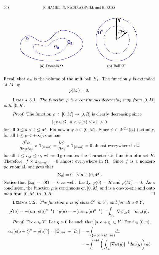
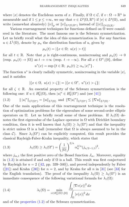
668 F. HAMEL, N. NADIRASHVILI, and E. RUSS
a
(a) Domain Ω
*
R
(b) Ball Ω∗
Recall that αn is the volume of the unit ball B1. The function ρ is extended
at M by
ρ(M) = 0.
Lemma 3.1. The function ρ is a continuous decreasing map from [0,M ]
onto [0, R].
Proof. The function ρ : [0,M ]→ [0, R] is clearly decreasing since
|x ∈ Ω, a < ψ(x) ≤ b| > 0
for all 0 ≤ a < b ≤ M . Fix now any a ∈ (0,M ]. Since ψ ∈ W 2,p(Ω) (actually,
for all 1 ≤ p < +∞), one has
∂2ψ
∂xi∂xj× 1ψ=a =
∂ψ
∂xi× 1ψ=a = 0 almost everywhere in Ω
for all 1 ≤ i, j ≤ n, where 1E denotes the characteristic function of a set E.
Therefore, f × 1ψ=a = 0 almost everywhere in Ω. Since f is a nonzero
polynomial, one gets that
|Σa| = 0 ∀ a ∈ (0,M ].
Notice that |Σ0| = |∂Ω| = 0 as well. Lastly, ρ(0) = R and ρ(M) = 0. As a
conclusion, the function ρ is continuous on [0,M ] and is a one-to-one and onto
map from [0,M ] to [0, R].
Lemma 3.2. The function ρ is of class C1 in Y , and for all a ∈ Y ,
ρ′(a) = −(nαnρ(a)n−1)−1g(a) = −(nαnρ(a)n−1)−1∫
Σa
|∇ψ(y)|−1dσa(y).
Proof. Fix a ∈ Y . Let η > 0 be such that [a, a+ η] ⊂ Y . For t ∈ (0, η),
αn[ρ(a+ t)n − ρ(a)n] = |Ωa+t| − |Ωa| = −∫a<ψ(x)≤a+t
dx
= −∫ a+t
a
Ç∫Σb
|∇ψ(y)|−1dσb(y)
ådb
REARRANGEMENT INEQUALITIES 669
from the coarea formula. Hence,
αn[ρ(a+ t)n − ρ(a)n]
t→ −g(a) as t→ 0+
for all a ∈ Y , due to the continuity of g on Y . Similarly, one has that
αn[ρ(a+ t)n − ρ(a)n]
t→ −g(a) as t→ 0−
for all a ∈ Y \0. The conclusion of the lemma follows since Y ⊂ [0,M),
whence ρ(a) 6= 0 for all a ∈ Y .
We now define the function ψ in Ω∗, which is a spherical rearrangement
of ψ by means of a new type of symmetrization. The definition of ψ involves
the rearrangement of the datum ΛΩ.
First, call
E = x ∈ Ω∗, |x| ∈ ρ(Y ).
The set E is a finite union of spherical shells and, from Lemma 3.1, it is open
relatively to Ω∗ and can be written as
E = x ∈ Rn, |x| ∈ (0, ρ(am−1)) ∪ · · · ∪ (ρ(a2), ρ(a1)) ∪ (ρ(a1), R],
with
0 = ρ(am) = ρ(M) < ρ(am−1) < · · · < ρ(a1) < R.
Notice that 0 6∈ E.
Next, for all r ∈ ρ(Y ), set
(3.3) G(r) =
∫Σρ−1(r)
|∇ψ(y)|−1 dσρ−1(r)∫Σρ−1(r)
ΛΩ(y)−1 |∇ψ(y)|−1 dσρ−1(r)
> 0,
where ρ−1 : [0, R] → [0,M ] denotes the reciprocal of the function ρ. For all
x ∈ E, define
(3.4) Λ(x) = G(|x|).
The function Λ is then defined almost everywhere in Ω∗. By the observations
above and since ΛΩ is positive and C1(Ω), the function Λ is continuous on E
and C1 on E ∩ Ω∗. Furthermore, Λ ∈ L∞(Ω∗) and
(3.5) 0 < minΩ
ΛΩ ≤ ess infΩ∗
Λ ≤ ess supΩ∗
Λ ≤ maxΩ
ΛΩ.
670 F. HAMEL, N. NADIRASHVILI, and E. RUSS
For any two real numbers a < b such that [a, b] ⊂ Y , the coarea formula gives∫Ωa\Ωb
ΛΩ(y)−1dy =
∫ b
a
Ç∫Σs
ΛΩ(y)−1|∇ψ(y)|−1dσs(y)
åds
=
∫ ρ(a)
ρ(b)
á∫Σρ−1(t)
ΛΩ(y)−1|∇ψ(y)|−1dσρ−1(t)(y)∫Σρ−1(t)
|∇ψ(y)|−1dσρ−1(t)(y)
ënαnt
n−1dt.
The last equality is obtained from Lemma 3.2 after the change of variables
s = ρ−1(t). Since Λ is radially symmetric, it follows by (3.3)–(3.4) that∫Ωa\Ωb
ΛΩ(y)−1dy =
∫Sρ(b),ρ(a)
Λ(x)−1dx,
where, for any 0 ≤ s < s′, Ss,s′ denotes
Ss,s′ = x ∈ Rn, s < |x| < s′.
Lebesgue’s dominated convergence theorem then implies that
(3.6)
∫Ω
ΛΩ(y)−1dy =
∫Ω∗
Λ(x)−1dx.
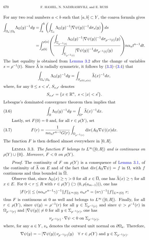
Lastly, set F (0) = 0 and, for all r ∈ ρ(Y ), set
(3.7) F (r) =1
nαnrn−1G(r)
∫Ωρ−1(r)
div(AΩ∇ψ)(x)dx.
The function F is then defined almost everywhere in [0, R].
Lemma 3.3. The function F belongs to L∞([0, R]) and is continuous on
ρ(Y ) ∪ 0. Moreover, F < 0 on ρ(Y ).
Proof. The continuity of F on ρ(Y ) is a consequence of Lemma 3.1, of
the continuity of Λ on E and of the fact that div(AΩ∇ψ) = f in Ω, with f
continuous and thus bounded in Ω.
Observe that, since ΛΩ(x) ≥ γ > 0 for all x ∈ Ω, one has Λ(x) ≥ γ for all
x ∈ E. For 0 < r ≤ R with r ∈ ρ(Y ) (⊃ (0, ρ(am−1))), one has
|F (r)| ≤ (nαnrn−1γ)−1‖f‖L∞(Ω) αnr
n = (nγ)−1‖f‖L∞(Ω) r;
thus F is continuous at 0 as well and belongs to L∞ ([0, R]). Finally, for all
r ∈ ρ(Y ), since ψ(y) = ρ−1(r) for all y ∈ Σρ−1(r) and since ψ > ρ−1(r) in
Ωρ−1(r) and |∇ψ(y)| 6= 0 for all y ∈ Σρ−1(r), one has
νρ−1(r) · ∇ψ < 0 on Σρ−1(r),
where, for any a ∈ Y , νa denotes the outward unit normal on ∂Ωa. Therefore,
∇ψ(y) = − |∇ψ(y)| νρ−1(r)(y) ∀ r ∈ ρ(Y ) and y ∈ Σρ−1(r).
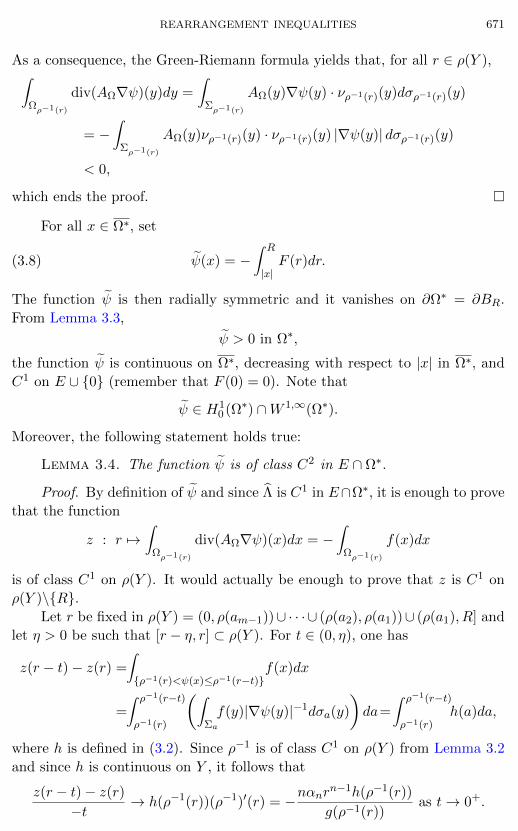
REARRANGEMENT INEQUALITIES 671
As a consequence, the Green-Riemann formula yields that, for all r ∈ ρ(Y ),∫Ωρ−1(r)
div(AΩ∇ψ)(y)dy =
∫Σρ−1(r)
AΩ(y)∇ψ(y) · νρ−1(r)(y)dσρ−1(r)(y)
= −∫
Σρ−1(r)
AΩ(y)νρ−1(r)(y) · νρ−1(r)(y) |∇ψ(y)| dσρ−1(r)(y)
< 0,
which ends the proof.
For all x ∈ Ω∗, set
(3.8) ψ(x) = −∫ R
|x|F (r)dr.
The function ψ is then radially symmetric and it vanishes on ∂Ω∗ = ∂BR.
From Lemma 3.3,
ψ > 0 in Ω∗,
the function ψ is continuous on Ω∗, decreasing with respect to |x| in Ω∗, and
C1 on E ∪ 0 (remember that F (0) = 0). Note that
ψ ∈ H10 (Ω∗) ∩W 1,∞(Ω∗).
Moreover, the following statement holds true:
Lemma 3.4. The function ψ is of class C2 in E ∩ Ω∗.
Proof. By definition of ψ and since Λ is C1 in E∩Ω∗, it is enough to prove
that the function
z : r 7→∫
Ωρ−1(r)
div(AΩ∇ψ)(x)dx = −∫
Ωρ−1(r)
f(x)dx
is of class C1 on ρ(Y ). It would actually be enough to prove that z is C1 on
ρ(Y )\R.Let r be fixed in ρ(Y ) = (0, ρ(am−1))∪ · · · ∪ (ρ(a2), ρ(a1))∪ (ρ(a1), R] and
let η > 0 be such that [r − η, r] ⊂ ρ(Y ). For t ∈ (0, η), one has
z(r − t)− z(r) =
∫ρ−1(r)<ψ(x)≤ρ−1(r−t)
f(x)dx
=
∫ ρ−1(r−t)
ρ−1(r)
Ç∫Σa
f(y)|∇ψ(y)|−1dσa(y)
åda=
∫ ρ−1(r−t)
ρ−1(r)h(a)da,
where h is defined in (3.2). Since ρ−1 is of class C1 on ρ(Y ) from Lemma 3.2
and since h is continuous on Y , it follows that
z(r − t)− z(r)−t
→ h(ρ−1(r))(ρ−1)′(r) = −nαnrn−1h(ρ−1(r))
g(ρ−1(r))as t→ 0+.
672 F. HAMEL, N. NADIRASHVILI, and E. RUSS
The same limit holds as t→ 0− for all r ∈ ρ(Y )\R. Therefore, the function
z is differentiable on ρ(Y ) and
z′(r) = −nαnrn−1h(ρ−1(r))
g(ρ−1(r))∀ r ∈ ρ(Y ).
Since ρ−1 is continuous on [0, R], and g and h are continuous on Y , the function
z is of class C1 on ρ(Y ). That completes the proof of Lemma 3.4.
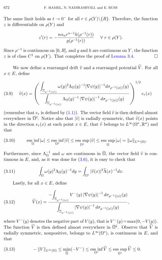
We now define a rearranged drift v and a rearranged potential “V . For all
x ∈ E, define
(3.9) v(x) =
á∫Σρ−1(|x|)
ω(y)2ΛΩ(y)−1|∇ψ(y)|−1dσρ−1(|x|)(y)∫Σρ−1(|x|)
ΛΩ(y)−1 |∇ψ(y)|−1 dσρ−1(|x|)(y)
ë1/2
er(x)
(remember that er is defined by (1.1)). The vector field v is then defined almost
everywhere in Ω∗. Notice also that |v| is radially symmetric, that v(x) points
in the direction er(x) at each point x ∈ E, that v belongs to L∞(Ω∗,Rn) and
that
(3.10) ess infΩ|ω| ≤ ess inf
Ω∗|v| ≤ ess sup
Ω∗|v| ≤ ess sup
Ω|ω| = ‖ω‖L∞(Ω).
Furthermore, since Λ−1Ω and ω are continuous in Ω, the vector field v is con-
tinuous in E, and, as it was done for (3.6), it is easy to check that
(3.11)
∫Ωω(y)2ΛΩ(y)−1dy =
∫Ω∗|v(x)|2Λ(x)−1dx.
Lastly, for all x ∈ E, define
(3.12) “V (x) =
−∫
Σρ−1(|x|)
V −(y) |∇ψ(y)|−1 dσρ−1(|x|)(y)∫Σρ−1(|x|)
|∇ψ(y)|−1 dσρ−1(|x|)(y),
where V −(y) denotes the negative part of V (y), that is V −(y)=max(0,−V (y)).
The function “V is then defined almost everywhere in Ω∗. Observe that “V is
radially symmetric, nonpositive, belongs to L∞(Ω∗), is continuous in E, and
that
(3.13) − ‖V ‖L∞(Ω) ≤ minΩ
(−V −) ≤ ess infΩ∗
“V ≤ ess supΩ∗
“V ≤ 0.
REARRANGEMENT INEQUALITIES 673
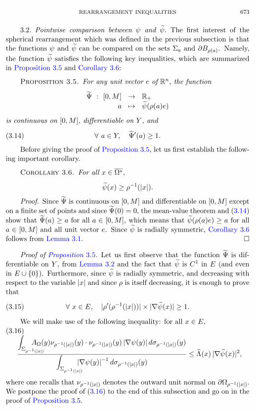
3.2. Pointwise comparison between ψ and ψ. The first interest of the
spherical rearrangement which was defined in the previous subsection is that
the functions ψ and ψ can be compared on the sets Σa and ∂Bρ(a). Namely,
the function ψ satisfies the following key inequalities, which are summarized
in Proposition 3.5 and Corollary 3.6:
Proposition 3.5. For any unit vector e of Rn, the function‹Ψ : [0,M ] → R+
a 7→ ψ(ρ(a)e)
is continuous on [0,M ], differentiable on Y , and
(3.14) ∀ a ∈ Y, ‹Ψ′(a) ≥ 1.
Before giving the proof of Proposition 3.5, let us first establish the follow-
ing important corollary.
Corollary 3.6. For all x ∈ Ω∗,
ψ(x) ≥ ρ−1(|x|).
Proof. Since ‹Ψ is continuous on [0,M ] and differentiable on [0,M ] except
on a finite set of points and since ‹Ψ(0) = 0, the mean-value theorem and (3.14)
show that ‹Ψ(a) ≥ a for all a ∈ [0,M ], which means that ψ(ρ(a)e) ≥ a for all
a ∈ [0,M ] and all unit vector e. Since ψ is radially symmetric, Corollary 3.6
follows from Lemma 3.1.
Proof of Proposition 3.5. Let us first observe that the function ‹Ψ is dif-
ferentiable on Y , from Lemma 3.2 and the fact that ψ is C1 in E (and even
in E ∪ 0). Furthermore, since ψ is radially symmetric, and decreasing with
respect to the variable |x| and since ρ is itself decreasing, it is enough to prove
that
(3.15) ∀ x ∈ E, |ρ′(ρ−1(|x|))| × |∇ψ(x)| ≥ 1.
We will make use of the following inequality: for all x ∈ E,
(3.16)∫Σρ−1(|x|)
AΩ(y)νρ−1(|x|)(y) · νρ−1(|x|)(y) |∇ψ(y)| dσρ−1(|x|)(y)∫Σρ−1(|x|)
|∇ψ(y)|−1 dσρ−1(|x|)(y)≤ Λ(x) |∇ψ(x)|2,
where one recalls that νρ−1(|x|) denotes the outward unit normal on ∂Ωρ−1(|x|).
We postpone the proof of (3.16) to the end of this subsection and go on in the
proof of Proposition 3.5.
674 F. HAMEL, N. NADIRASHVILI, and E. RUSS
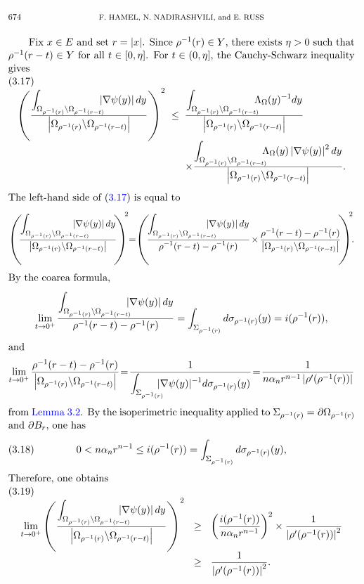
Fix x ∈ E and set r = |x|. Since ρ−1(r) ∈ Y , there exists η > 0 such that
ρ−1(r − t) ∈ Y for all t ∈ [0, η]. For t ∈ (0, η], the Cauchy-Schwarz inequality
gives
(3.17)á∫Ωρ−1(r)\Ωρ−1(r−t)
|∇ψ(y)| dy∣∣∣Ωρ−1(r)\Ωρ−1(r−t)
∣∣∣ë2
≤
∫Ωρ−1(r)\Ωρ−1(r−t)
ΛΩ(y)−1dy∣∣∣Ωρ−1(r)\Ωρ−1(r−t)
∣∣∣×
∫Ωρ−1(r)\Ωρ−1(r−t)
ΛΩ(y) |∇ψ(y)|2 dy∣∣∣Ωρ−1(r)\Ωρ−1(r−t)
∣∣∣ .
The left-hand side of (3.17) is equal toá∫Ωρ−1(r)\Ωρ−1(r−t)
|∇ψ(y)| dy∣∣Ωρ−1(r)\Ωρ−1(r−t)∣∣ë2
=
á∫Ωρ−1(r)\Ωρ−1(r−t)
|∇ψ(y)| dy
ρ−1(r − t)− ρ−1(r)× ρ−1(r − t)− ρ−1(r)∣∣Ωρ−1(r)\Ωρ−1(r−t)
∣∣ë2
.
By the coarea formula,
limt→0+
∫Ωρ−1(r)\Ωρ−1(r−t)
|∇ψ(y)| dy
ρ−1(r − t)− ρ−1(r)=
∫Σρ−1(r)
dσρ−1(r)(y) = i(ρ−1(r)),
and
limt→0+
ρ−1(r − t)− ρ−1(r)∣∣∣Ωρ−1(r)\Ωρ−1(r−t)
∣∣∣ =1∫
Σρ−1(r)
|∇ψ(y)|−1dσρ−1(r)(y)=
1
nαnrn−1 |ρ′(ρ−1(r))|
from Lemma 3.2. By the isoperimetric inequality applied to Σρ−1(r) = ∂Ωρ−1(r)
and ∂Br, one has
(3.18) 0 < nαnrn−1 ≤ i(ρ−1(r)) =
∫Σρ−1(r)
dσρ−1(r)(y),
Therefore, one obtains
(3.19)
limt→0+
á∫Ωρ−1(r)\Ωρ−1(r−t)
|∇ψ(y)| dy∣∣∣Ωρ−1(r)\Ωρ−1(r−t)
∣∣∣ë2
≥Çi(ρ−1(r))
nαnrn−1
å2
× 1
|ρ′(ρ−1(r))|2
≥ 1
|ρ′(ρ−1(r))|2.
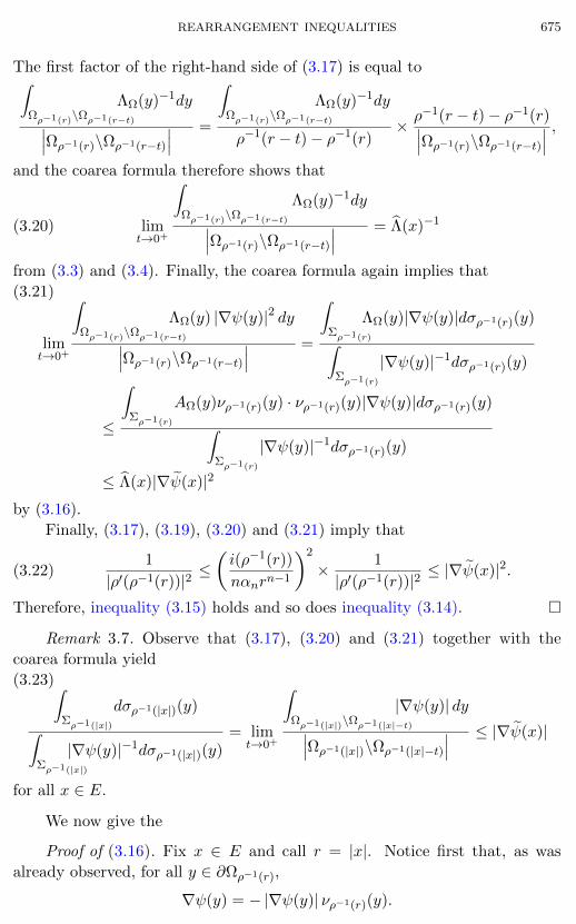
REARRANGEMENT INEQUALITIES 675
The first factor of the right-hand side of (3.17) is equal to∫Ωρ−1(r)\Ωρ−1(r−t)
ΛΩ(y)−1dy∣∣∣Ωρ−1(r)\Ωρ−1(r−t)
∣∣∣ =
∫Ωρ−1(r)\Ωρ−1(r−t)
ΛΩ(y)−1dy
ρ−1(r − t)− ρ−1(r)× ρ−1(r − t)− ρ−1(r)∣∣∣Ωρ−1(r)\Ωρ−1(r−t)
∣∣∣ ,and the coarea formula therefore shows that
(3.20) limt→0+
∫Ωρ−1(r)\Ωρ−1(r−t)
ΛΩ(y)−1dy∣∣∣Ωρ−1(r)\Ωρ−1(r−t)
∣∣∣ = Λ(x)−1
from (3.3) and (3.4). Finally, the coarea formula again implies that
(3.21)
limt→0+
∫Ωρ−1(r)\Ωρ−1(r−t)
ΛΩ(y) |∇ψ(y)|2 dy∣∣∣Ωρ−1(r)\Ωρ−1(r−t)
∣∣∣ =
∫Σρ−1(r)
ΛΩ(y)|∇ψ(y)|dσρ−1(r)(y)∫Σρ−1(r)
|∇ψ(y)|−1dσρ−1(r)(y)
≤
∫Σρ−1(r)
AΩ(y)νρ−1(r)(y) · νρ−1(r)(y)|∇ψ(y)|dσρ−1(r)(y)∫Σρ−1(r)
|∇ψ(y)|−1dσρ−1(r)(y)
≤ Λ(x)|∇ψ(x)|2
by (3.16).
Finally, (3.17), (3.19), (3.20) and (3.21) imply that
(3.22)1
|ρ′(ρ−1(r))|2≤Çi(ρ−1(r))
nαnrn−1
å2
× 1
|ρ′(ρ−1(r))|2≤ |∇ψ(x)|2.
Therefore, inequality (3.15) holds and so does inequality (3.14).
Remark 3.7. Observe that (3.17), (3.20) and (3.21) together with the
coarea formula yield
(3.23)∫Σρ−1(|x|)
dσρ−1(|x|)(y)∫Σρ−1(|x|)
|∇ψ(y)|−1dσρ−1(|x|)(y)= lim
t→0+
∫Ωρ−1(|x|)\Ωρ−1(|x|−t)
|∇ψ(y)| dy∣∣∣Ωρ−1(|x|)\Ωρ−1(|x|−t)
∣∣∣ ≤ |∇ψ(x)|
for all x ∈ E.
We now give the
Proof of (3.16). Fix x ∈ E and call r = |x|. Notice first that, as was
already observed, for all y ∈ ∂Ωρ−1(r),
∇ψ(y) = − |∇ψ(y)| νρ−1(r)(y).
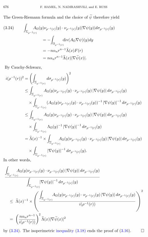
676 F. HAMEL, N. NADIRASHVILI, and E. RUSS
The Green-Riemann formula and the choice of ψ therefore yield∫Σρ−1(r)
AΩ(y)νρ−1(r)(y) · νρ−1(r)(y)|∇ψ(y)|dσρ−1(r)(y)(3.24)
= −∫
Ωρ−1(r)
div(AΩ∇ψ)(y)dy
= −nαnrn−1Λ(x)F (r)
= nαnrn−1Λ(x)|∇ψ(x)|.
By Cauchy-Schwarz,
i(ρ−1(r))2 =
(∫Σρ−1(r)
dσρ−1(r)(y)
)2
≤∫
Σρ−1(r)
AΩ(y)νρ−1(r)(y) · νρ−1(r)(y) |∇ψ(y)| dσρ−1(r)(y)
×∫
Σρ−1(r)
(AΩ(y)νρ−1(r)(y) · νρ−1(r)(y))−1 |∇ψ(y)|−1 dσρ−1(r)(y)
≤∫
Σρ−1(r)
AΩ(y)νρ−1(r)(y) · νρ−1(r)(y) |∇ψ(y)| dσρ−1(r)(y)
×∫
Σρ−1(r)
ΛΩ(y)−1 |∇ψ(y)|−1 dσρ−1(r)(y)
= Λ(x)−1 ×∫
Σρ−1(r)
AΩ(y)νρ−1(r)(y) · νρ−1(r)(y) |∇ψ(y)| dσρ−1(r)(y)
×∫
Σρ−1(r)
|∇ψ(y)|−1 dσρ−1(r)(y).
In other words,∫Σρ−1(r)
AΩ(y)νρ−1(r)(y) · νρ−1(r)(y) |∇ψ(y)| dσρ−1(r)(y)∫Σρ−1(r)
|∇ψ(y)|−1 dσρ−1(r)(y)
≤ Λ(x)−1 ×
á∫Σρ−1(r)
AΩ(y)νρ−1(r)(y) · νρ−1(r)(y) |∇ψ(y)| dσρ−1(r)(y)
i(ρ−1(r))
ë2
=
Çnαnr
n−1
i(ρ−1(r))
å2
Λ(x)|∇ψ(x)|2
by (3.24). The isoperimetric inequality (3.18) ends the proof of (3.16).
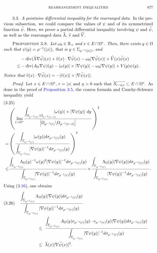
REARRANGEMENT INEQUALITIES 677
3.3. A pointwise differential inequality for the rearranged data. In the pre-
vious subsection, we could compare the values of ψ and of its symmetrized
function ψ. Here, we prove a partial differential inequality involving ψ and ψ,
as well as the rearranged data Λ, v and “V .
Proposition 3.8. Let ω0 ∈ R+ and x ∈ E∩Ω∗. Then, there exists y ∈ Ω
such that ψ(y) = ρ−1(|x|), that is y ∈ Σρ−1(|x|), and
− div(Λ∇ψ)(x) + v(x) · ∇ψ(x)− ω0|∇ψ(x)|+ “V (x)ψ(x)
≤− div(AΩ∇ψ)(y)− |ω(y)| × |∇ψ(y)| − ω0|∇ψ(y)|+ V (y)ψ(y).
Notice that v(x) · ∇ψ(x) = −|v(x)| × |∇ψ(x)|.
Proof. Let x ∈ E ∩ Ω∗, r = |x| and η > 0 such that Sr−η,r ⊂ E ∩ Ω∗. As
done in the proof of Proposition 3.5, the coarea formula and Cauchy-Schwarz
inequality yieldálimt→0+
∫Ωρ−1(r)\Ωρ−1(r−t)
|ω(y)| × |∇ψ(y)| dy∣∣∣Ωρ−1(r)\Ωρ−1(r−t)
∣∣∣ë2
(3.25)
=
á ∫Σρ−1(r)
|ω(y)|dσρ−1(r)(y)∫Σρ−1(r)
|∇ψ(y)|−1dσρ−1(r)(y)
ë2
≤
∫Σρ−1(r)
ΛΩ(y)−1ω(y)2|∇ψ(y)|−1dσρ−1(r)(y)∫Σρ−1(r)
|∇ψ(y)|−1dσρ−1(r)(y)×
∫Σρ−1(r)
ΛΩ(y)|∇ψ(y)|dσρ−1(r)(y)∫Σρ−1(r)
|∇ψ(y)|−1dσρ−1(r)(y).
Using (3.16), one obtains∫Σρ−1(r)
ΛΩ(y)|∇ψ(y)|dσρ−1(r)(y)∫Σρ−1(r)
|∇ψ(y)|−1dσρ−1(r)(y)(3.26)
≤
∫Σρ−1(r)
AΩ(y)νρ−1(r)(y) · νρ−1(r)(y)|∇ψ(y)|dσρ−1(r)(y)∫Σρ−1(r)
|∇ψ(y)|−1dσρ−1(r)(y)
≤ Λ(x)|∇ψ(x)|2.
678 F. HAMEL, N. NADIRASHVILI, and E. RUSS
Finally, (3.25) and (3.26), together with definitions (3.3)–(3.4) and (3.9), give
that
(3.27)
limt→0+
∫Ωρ−1(r)\Ωρ−1(r−t)
|ω(y)| × |∇ψ(y)| dy∣∣∣Ωρ−1(r)\Ωρ−1(r−t)
∣∣∣ ≤ |v(x)| × |∇ψ(x)| = −v(x) · ∇ψ(x).
The last equality follows also from (3.8) and Lemma 3.3.
Remember also from (3.23) that
(3.28) limt→0+
∫Ωρ−1(r)\Ωρ−1(r−t)
|∇ψ(y)| dy∣∣∣Ωρ−1(r)\Ωρ−1(r−t)
∣∣∣ ≤ |∇ψ(x)| = −er(x) · ∇ψ(x).
As far as V is concerned, for any fixed unit vector e in Rn and for any
t ∈ (0, η), it follows from (3.12) and Lemma 3.2 that∫Ωρ−1(r)\Ωρ−1(r−t)
V (y)ψ(y)dy
≥∫ ρ−1(r−t)
ρ−1(r)
Ç∫Σa
(−V −(y))ψ(y) |∇ψ(y)|−1 dσa(y)
åda
= −∫ ρ−1(r−t)
ρ−1(r)a
Ç∫Σa
V −(y) |∇ψ(y)|−1 dσa(y)
åda
= −∫ r
r−t
(∫Σρ−1(s)
V −(y) |∇ψ(y)|−1 dσρ−1(s)(y)
)ρ−1(s)ds
|ρ′(ρ−1(s))|
= −nαn∫ r
r−tsn−1ρ−1(s)
á∫Σρ−1(s)
V −(y) |∇ψ(y)|−1 dσρ−1(s)(y)∫Σρ−1(s)
|∇ψ(y)|−1 dσρ−1(s)(y)
ëds
= nαn
∫ r
r−tsn−1ρ−1(s)“V (se)ds.
Moreover, the radial symmetry of “V and ψ yields∫Sr−t,r
“V (y)ψ(y)dy = nαn
∫ r
r−tsn−1“V (se)ψ(se)ds.
Corollary 3.6 and the facts that∣∣∣Ωρ−1(r)\Ωρ−1(r−t)
∣∣∣ = |Sr−t,r| and that “V ≤ 0
therefore show that∫Ωρ−1(r)\Ωρ−1(r−t)
V (y)ψ(y)dy∣∣∣Ωρ−1(r)\Ωρ−1(r−t)
∣∣∣ ≥
∫Sr−t,r
“V (y)ψ(y)dy
|Sr−t,r|.
REARRANGEMENT INEQUALITIES 679
Since “V and ψ are continuous in E and radially symmetric, one therefore
obtains, together with the coarea formula,
(3.29)∫Σρ−1(r)
V (y)ψ(y)|∇ψ(y)|−1dσρ−1(r)(y)∫Σρ−1(r)
|∇ψ(y)|−1dσρ−1(r)(y)= lim
t→0+
∫Ωρ−1(r)\Ωρ−1(r−t)
V (y)ψ(y)dy∣∣∣Ωρ−1(r)\Ωρ−1(r−t)
∣∣∣≥ “V (x)ψ(x).
Let now t be any real number in (0, η). Since ψ (resp. Λ) is radially
symmetric and C2 (resp. C1) on Sr−t,r ⊂ E ∩Ω∗, the Green Riemann formula
gives
(3.30)∫Sr−t,r
div(Λ∇ψ)(y)dy =
∫∂Sr−t,r
Λ(y)∇ψ(y) · ν(y)dσ(y)
= nαn [rn−1G(r)F (r)− (r − t)n−1G(r − t)F (r − t)],
where dσ and ν here denote the superficial measure on ∂Sr−t,r and the out-
ward unit normal to Sr−t,r, and G and F were defined in (3.3) and (3.7). By
definition of F , one gets that∫Sr−t,r
div(Λ∇ψ)(y)dy =
∫Ωρ−1(r)\Ωρ−1(r−t)
div(AΩ∇ψ)(y)dy,
whence
(3.31)∫Σρ−1(r)
div(AΩ∇ψ)(y)|∇ψ(y)|−1dσρ−1(r)(y)∫Σρ−1(r)
|∇ψ(y)|−1dσρ−1(r)(y)
= limt→0+
∫Ωρ−1(r)\Ωρ−1(r−t)
div(AΩ∇ψ)(y)dy∣∣∣Ωρ−1(r)\Ωρ−1(r−t)
∣∣∣ = div(Λ∇ψ)(x)
since |Sr−t,r| =∣∣∣Ωρ−1(r)\Ωρ−1(r−t)
∣∣∣.It follows from (3.27), (3.28), (3.29) and (3.31) that
limt→0+
∫Ωρ−1(r)\Ωρ−1(r−t)
[div(AΩ∇ψ)(y) + |ω(y)| × |∇ψ(y)|+ ω0|∇ψ(y)| − V (y)ψ(y)] dy∣∣Ωρ−1(r)\Ωρ−1(r−t)∣∣
≤ div(Λ∇ψ)(x)− v(x) · ∇ψ(x) + ω0|∇ψ(x)| − “V (x)ψ(x).
To finish the proof, pick any sequence of positive numbers (εl)l∈N such that
εl → 0 as l→ +∞. Since ψ is C2 in Ω, since AΩ is C1 in Ω (and even in Ω) and
680 F. HAMEL, N. NADIRASHVILI, and E. RUSS
ω and V are continuous in Ω (and even in Ω), the previous inequality provides
the existence of a sequence of positive real numbers (tl)l∈N ∈ (0, η) such that
tl → 0 as l→ +∞, and a sequence of points
yl ∈ Ωρ−1(r)\Ωρ−1(r−tl) ⊂ Ωρ−1(r) ⊂ Ω
such that
div(AΩ∇ψ)(yl) + |ω(yl)| × |∇ψ(yl)|+ ω0|∇ψ(yl)| − V (yl)ψ(yl)
≤ div(Λ∇ψ)(x)− v(x) · ∇ψ(x) + ω0|∇ψ(x)| − “V (x)ψ(x) + εl.
Since ρ−1(r) ≤ ψ(yl) ≤ ρ−1(r−tl) and ρ−1 is continuous, the points yl converge,
up to the extraction of some subsequence, to a point y ∈ Σρ−1(r) such that
div(AΩ∇ψ)(y) + |ω(y)| × |∇ψ(y)|+ ω0|∇ψ(y)| − V (y)ψ(y)
≤ div(Λ∇ψ)(x)− v(x) · ∇ψ(x) + ω0|∇ψ(x)| − “V (x)ψ(x),
which is the conclusion of Proposition 3.8.
Corollary 3.9. If there are ω0 ≥ 0 and µ ≥ 0 such that
−div(AΩ∇ψ)(y)− |ω(y)|×|∇ψ(y)| − ω0|∇ψ(y)|+ V (y)ψ(y) ≤ µψ(y) ∀ y ∈ Ω,
then
−div(Λ∇ψ)(x) + v(x)·∇ψ(x)− ω0|∇ψ(x)|+ “V (x)ψ(x) ≤ µψ(x) ∀ x ∈ E ∩Ω∗.
Proof. It follows immediately from Corollary 3.6 and Proposition 3.8.
3.4. An integral inequality for the rearranged data. A consequence of the
pointwise comparisons which were established in the previous subsections is
the following integral comparison result:
Proposition 3.10. With the previous notation, assume that, for some
(ω0, µ) ∈ R2,
(3.32)
− div(Λ∇ψ)(x)+v(x)·∇ψ(x)−ω0|∇ψ(x)|+“V (x)ψ(x) ≤ µψ(x) ∀ x ∈ E ∩Ω∗.
Fix a unit vector e ∈ Rn. For all r ∈ [0, R], define
(3.33) H(r) =
∫ r
0|v(se)| Λ(se)−1ds
and, for all x ∈ Ω∗, let
(3.34) U(x) = H(|x|).
Then, the following integral inequality is valid :∫Ω∗
îΛ(x)|∇ψ(x)|2−ω0|∇ψ(x)|ψ(x)+“V (x)ψ(x)2
óe−U(x)dx(3.35)
≤ µ∫
Ω∗ψ(x)2e−U(x)dx.
REARRANGEMENT INEQUALITIES 681
Proof. Note first that, since |v| and Λ are radially symmetric and since
|v| ∈ L∞(Ω∗) and Λ satisfies (3.5), the function H is well defined and contin-
uous in [0, R]. Furthermore, its definition is independent from the choice of
e. The radially symmetric function U is then continuous in Ω∗ and, since the
radially symmetric functions v = |v|er and 1/Λ are (at least) continuous in E,
the function U is of class C1 in E and
(3.36) ∇U(x) = Λ(x)−1v(x) ∀ x ∈ E.
Observe also that the integrals in (3.35) are all well defined since ψ ∈ H10 (Ω∗)
and Λ, “V , U ∈ L∞(Ω∗) (even, U ∈ C(Ω∗)).
Now, recall that the set of critical values of ψ is Z = a1, . . . , am with
0 < a1 < · · · < am = M
and remember that the function ρ defined in Section 3.1 is continuous and
decreasing from [0,M ] onto [0, R], from Lemma 3.1. Fix j ∈ 1, . . . ,m− 1and r, r′ such that
0 ≤ ρ(aj+1) < r < r′ < ρ(aj) < R.
Multiplying (3.32) by the nonnegative function ψe−U and integrating over Sr,r′
yields
(3.37)∫Sr,r′
î−div(Λ∇ψ)(x) + v(x)·∇ψ(x)− ω0|∇ψ(x)|+ “V (x)ψ(x)
óψ(x) e−U(x) dx
≤ µ
∫Sr,r′
ψ(x)2e−U(x)dx.
Notice that all integrals above are well defined since ψ in C2 in E∩Ω∗, Λ is C1
in E ∩Ω∗, v, “V are continuous in E, U is continuous in Ω∗ and Sr,r′ ⊂ E ∩Ω∗.
Furthermore, as in (3.30), the Green-Riemann formula yields∫Sr,r′−div(Λ∇ψ)(x) ψ(x) e−U(x) dx
=
∫Sr,r′
Λ(x) |∇ψ(x)|2 e−U(x) dx−∫Sr,r′
Λ(x) ψ(x)∇ψ(x) · ∇U(x) e−U(x) dx
− nαn(r′)n−1G(r′)F (r′)ψ(r′e) e−H(r′) + nαnrn−1G(r)F (r)ψ(re) e−H(r).
By (3.36), it follows then that
(3.38)∫Sr,r′
î−div(Λ∇ψ)(x) + v(x)·∇ψ(x)− ω0|∇ψ(x)|+ “V (x)ψ(x)
óψ(x) e−U(x) dx
=
∫Sr,r′
îΛ(x)|∇ψ(x)|2 − ω0|∇ψ(x)|ψ(x) + “V (x)ψ(x)2
óe−U(x) dx
− nαn(r′)n−1G(r′)F (r′)ψ(r′e) e−H(r′) + nαnrn−1G(r)F (r)ψ(re) e−H(r).
682 F. HAMEL, N. NADIRASHVILI, and E. RUSS
On the other hand, for all s ∈ ρ(Y ),
nαnsn−1F (s)G(s) =
∫Ωρ−1(s)
div(AΩ∇ψ)(x)dx,
by (3.7). The function
s 7→ I(s) = nαnsn−1F (s)G(s),
which was a priori defined only in ρ(Y ), can then be extended continuously in
[0, R] from the results in Lemma 3.1 and since div(AΩ∇ψ) = −f is bounded
in Ω. The continuous extension of I in [0, R] is still called I. Passing to the
limit as r → ρ(aj+1)+ and r′ → ρ(aj)− in (3.37) and (3.38) yields, for each
j ∈ 1, . . . ,m− 1,∫Sρ(aj+1),ρ(aj)
îΛ(x)|∇ψ(x)|2 − ω0|∇ψ(x)|ψ(x) + “V (x)ψ(x)2
óe−U(x) dx(3.39)
− I(ρ(aj)) ψ(ρ(aj)e) e−H(ρ(aj)) + I(ρ(aj+1)) ψ(ρ(aj+1)e) e−H(ρ(aj+1))
≤ µ∫Sρ(aj+1),ρ(aj)
ψ(x)2e−U(x) dx.
Once again, all integrals above are well defined. Arguing similarly in the
spherical shell Sρ(a1),R and since ψ(Re) = 0, one obtains∫Sρ(a1),R
îΛ(x)|∇ψ(x)|2 − ω0|∇ψ(x)|ψ(x) + “V (x)ψ(x)2
óe−U(x) dx(3.40)
+ I(ρ(a1)) ψ(ρ(a1)e) e−H(ρ(a1)) ≤ µ∫Sρ(a1),R
ψ(x)2e−U(x)dx.
Summing up (3.39) for all 1 ≤ j ≤ m − 1 and (3.40) and using the fact that
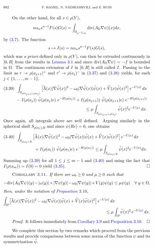
I(ρ(am)) = I(0) = 0 yield (3.35).
Corollary 3.11. If there are ω0 ≥ 0 and µ ≥ 0 such that
−div(AΩ∇ψ)(y)−|ω(y)|×|∇ψ(y)|−ω0|∇ψ(y)|+V (y)ψ(y) ≤ µψ(y) ∀ y ∈ Ω,
then, under the notation of Proposition 3.10,∫Ω∗
îΛ(x)|∇ψ(x)|2 − ω0|∇ψ(x)|ψ(x) + “V (x)ψ(x)2
óe−U(x) dx
≤ µ∫
Ω∗ψ(x)2 e−U(x) dx.
Proof. It follows immediately from Corollary 3.9 and Proposition 3.10.
We complete this section by two remarks which proceed from the previous
results and provide comparisons between some norms of the function ψ and its
symmetrization ψ.
REARRANGEMENT INEQUALITIES 683
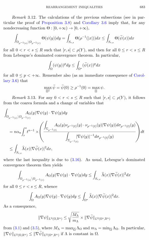
Remark 3.12. The calculations of the previous subsections (see in par-
ticular the proof of Proposition 3.8) and Corollary 3.6 imply that, for any
nondecreasing function Θ : [0,+∞)→ [0,+∞),∫Ωρ−1(s)\Ωρ−1(r)
Θ(ψ(y))dy =
∫Sr,s
Θ(ρ−1(|x|))dx ≤∫Sr,s
Θ(ψ(x))dx
for all 0 < r < s ≤ R such that [r, s] ⊂ ρ(Y ), and then for all 0 ≤ r < s ≤ R
from Lebesgue’s dominated convergence theorem. In particular,∫Ω
(ψ(y))pdy ≤∫
Ω∗(ψ(x))pdx
for all 0 ≤ p < +∞. Remember also (as an immediate consequence of Corol-
lary 3.6) that
maxΩ∗
ψ = ψ(0) ≥ ρ−1(0) = maxΩ
ψ.
Remark 3.13. For any 0 < r < s ≤ R such that [r, s] ⊂ ρ(Y ), it follows
from the coarea formula and a change of variables that∫Ωρ−1(s)\Ωρ−1(r)
AΩ(y)∇ψ(y) · ∇ψ(y)dy
= nαn
∫ s
rtn−1 ×
á∫Σρ−1(t)
AΩ(y)νρ−1(t)(y) · νρ−1(t)(y)|∇ψ(y)|dσρ−1(t)(y)∫Σρ−1(t)
|∇ψ(y)|−1dσρ−1(t)(y)
ëdt
≤∫Sr,s
Λ(x)|∇ψ(x)|2dx,
where the last inequality is due to (3.16). As usual, Lebesgue’s dominated
convergence theorem then yields∫Ωρ−1(s)\Ωρ−1(r)
AΩ(y)∇ψ(y) · ∇ψ(y)dy ≤∫Sr,s
Λ(x)|∇ψ(x)|2dx
for all 0 ≤ r < s ≤ R, whence∫ΩAΩ(y)∇ψ(y) · ∇ψ(y)dy ≤
∫Ω∗
Λ(x)|∇ψ(x)|2dx.
As a consequence,
‖∇ψ‖L2(Ω,Rn) ≤ MΛ
mΛ× ‖∇ψ‖L2(Ω∗,Rn)
from (3.1) and (3.5), where MΛ = maxΩ ΛΩ and mΛ = minΩ ΛΩ. In particular,
‖∇ψ‖L2(Ω,Rn) ≤ ‖∇ψ‖L2(Ω∗,Rn) if Λ is constant in Ω.
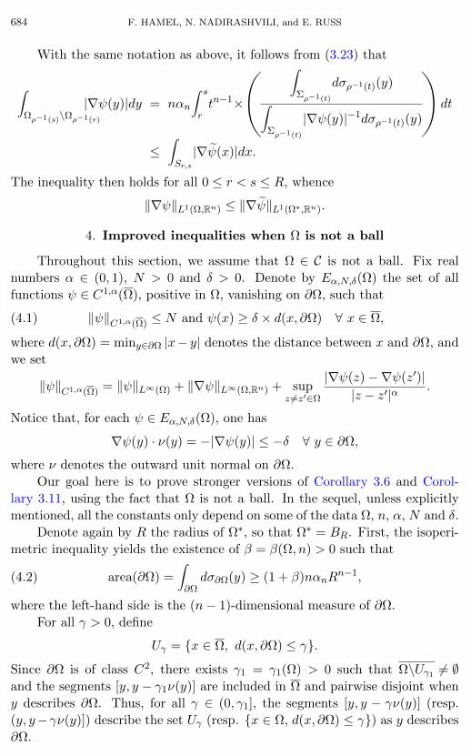
684 F. HAMEL, N. NADIRASHVILI, and E. RUSS
With the same notation as above, it follows from (3.23) that
∫Ωρ−1(s)\Ωρ−1(r)
|∇ψ(y)|dy = nαn
∫ s
rtn−1×
á ∫Σρ−1(t)
dσρ−1(t)(y)∫Σρ−1(t)
|∇ψ(y)|−1dσρ−1(t)(y)
ëdt
≤∫Sr,s
|∇ψ(x)|dx.
The inequality then holds for all 0 ≤ r < s ≤ R, whence
‖∇ψ‖L1(Ω,Rn) ≤ ‖∇ψ‖L1(Ω∗,Rn).
4. Improved inequalities when Ω is not a ball
Throughout this section, we assume that Ω ∈ C is not a ball. Fix real
numbers α ∈ (0, 1), N > 0 and δ > 0. Denote by Eα,N,δ(Ω) the set of all
functions ψ ∈ C1,α(Ω), positive in Ω, vanishing on ∂Ω, such that
(4.1) ‖ψ‖C1,α(Ω) ≤ N and ψ(x) ≥ δ × d(x, ∂Ω) ∀ x ∈ Ω,
where d(x, ∂Ω) = miny∈∂Ω |x− y| denotes the distance between x and ∂Ω, and
we set
‖ψ‖C1,α(Ω) = ‖ψ‖L∞(Ω) + ‖∇ψ‖L∞(Ω,Rn) + supz 6=z′∈Ω
|∇ψ(z)−∇ψ(z′)||z − z′|α
.
Notice that, for each ψ ∈ Eα,N,δ(Ω), one has
∇ψ(y) · ν(y) = −|∇ψ(y)| ≤ −δ ∀ y ∈ ∂Ω,
where ν denotes the outward unit normal on ∂Ω.
Our goal here is to prove stronger versions of Corollary 3.6 and Corol-
lary 3.11, using the fact that Ω is not a ball. In the sequel, unless explicitly
mentioned, all the constants only depend on some of the data Ω, n, α, N and δ.
Denote again by R the radius of Ω∗, so that Ω∗ = BR. First, the isoperi-
metric inequality yields the existence of β = β(Ω, n) > 0 such that
(4.2) area(∂Ω) =
∫∂Ωdσ∂Ω(y) ≥ (1 + β)nαnR
n−1,
where the left-hand side is the (n− 1)-dimensional measure of ∂Ω.
For all γ > 0, define
Uγ = x ∈ Ω, d(x, ∂Ω) ≤ γ.
Since ∂Ω is of class C2, there exists γ1 = γ1(Ω) > 0 such that Ω\Uγ1 6= ∅and the segments [y, y − γ1ν(y)] are included in Ω and pairwise disjoint when
y describes ∂Ω. Thus, for all γ ∈ (0, γ1], the segments [y, y − γν(y)] (resp.
(y, y−γν(y)]) describe the set Uγ (resp. x ∈ Ω, d(x, ∂Ω) ≤ γ) as y describes
∂Ω.
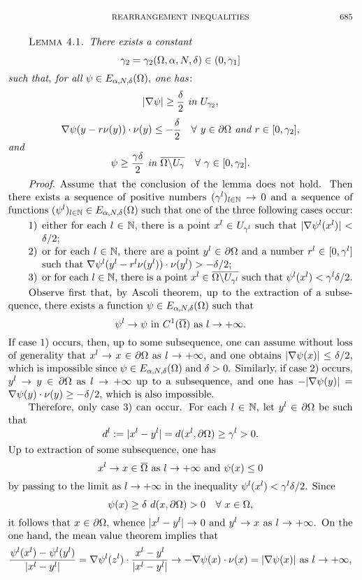
REARRANGEMENT INEQUALITIES 685
Lemma 4.1. There exists a constant
γ2 = γ2(Ω, α,N, δ) ∈ (0, γ1]
such that, for all ψ ∈ Eα,N,δ(Ω), one has :
|∇ψ| ≥ δ
2in Uγ2 ,
∇ψ(y − rν(y)) · ν(y) ≤ −δ2∀ y ∈ ∂Ω and r ∈ [0, γ2],
and
ψ ≥ γδ
2in Ω\Uγ ∀ γ ∈ [0, γ2].
Proof. Assume that the conclusion of the lemma does not hold. Then
there exists a sequence of positive numbers (γl)l∈N → 0 and a sequence of
functions (ψl)l∈N ∈ Eα,N,δ(Ω) such that one of the three following cases occur:
1) either for each l ∈ N, there is a point xl ∈ Uγl such that |∇ψl(xl)| <δ/2;
2) or for each l ∈ N, there are a point yl ∈ ∂Ω and a number rl ∈ [0, γl]
such that ∇ψl(yl − rlν(yl)) · ν(yl) > −δ/2;
3) or for each l ∈ N, there is a point xl ∈ Ω\Uγl such that ψl(xl) < γlδ/2.
Observe first that, by Ascoli theorem, up to the extraction of a subse-
quence, there exists a function ψ ∈ Eα,N,δ(Ω) such that
ψl → ψ in C1(Ω) as l→ +∞.
If case 1) occurs, then, up to some subsequence, one can assume without loss
of generality that xl → x ∈ ∂Ω as l → +∞, and one obtains |∇ψ(x)| ≤ δ/2,
which is impossible since ψ ∈ Eα,N,δ(Ω) and δ > 0. Similarly, if case 2) occurs,
yl → y ∈ ∂Ω as l → +∞ up to a subsequence, and one has −|∇ψ(y)| =
∇ψ(y) · ν(y) ≥ −δ/2, which is also impossible.
Therefore, only case 3) can occur. For each l ∈ N, let yl ∈ ∂Ω be such
that
dl := |xl − yl| = d(xl, ∂Ω) ≥ γl > 0.
Up to extraction of some subsequence, one has
xl → x ∈ Ω as l→ +∞ and ψ(x) ≤ 0
by passing to the limit as l→ +∞ in the inequality ψl(xl) < γlδ/2. Since
ψ(x) ≥ δ d(x, ∂Ω) > 0 ∀ x ∈ Ω,
it follows that x ∈ ∂Ω, whence |xl − yl| → 0 and yl → x as l → +∞. On the
one hand, the mean value theorem implies that
ψl(xl)− ψl(yl)|xl − yl|
= ∇ψl(zl) · xl − yl
|xl − yl|→ −∇ψ(x) · ν(x) = |∇ψ(x)| as l→ +∞,
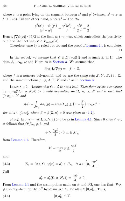
686 F. HAMEL, N. NADIRASHVILI, and E. RUSS
where zl is a point lying on the segment between xl and yl (whence, zl → x as
l→ +∞). On the other hand, since ψl = 0 on ∂Ω,
ψl(xl)− ψl(yl)|xl − yl|
=ψl(xl)
dl<γlδ
2γl=δ
2.
Hence, |∇ψ(x)| ≤ δ/2 at the limit as l→ +∞, which contradicts the positivity
of δ and the fact that ψ ∈ Eα,N,δ(Ω).
Therefore, case 3) is ruled out too and the proof of Lemma 4.1 is complete.
In the sequel, we assume that ψ ∈ Eα,N,δ(Ω) and is analytic in Ω. The
data AΩ, ΛΩ, ω and V are as in Section 3. We assume that
div(AΩ∇ψ) = −f in Ω,
where f is a nonzero polynomial, and we use the same sets Z, Y , E, Ωa, Σa
and the same functions ρ, ψ, Λ, v, “V and U as in Section 3.
Lemma 4.2. Assume that Ω ∈ C is not a ball. Then there exists a constant
a0 = a0(Ω, n, α,N, δ) > 0 only depending on Ω, n, α, N and δ such that
[0, a0] ⊂ Y and
i(a) =
∫Σa
dσa(y) = area(Σa) ≥Å
1 +β
2
ãnαnR
n−1
for all a ∈ [0, a0], where β = β(Ω, n) > 0 was given in (4.2).
Proof. Let γ2 = γ2(Ω, α,N, δ) > 0 be as in Lemma 4.1. Since 0 < γ2 ≤ γ1,
it follows that Ω\Uγ2 6= ∅, and
ψ ≥ γ2δ
2> 0 in Ω\Uγ2
from Lemma 4.1. Therefore,
M = maxΩ
ψ ≥ γ2δ
2
and
(4.3) Σa = x ∈ Ω, ψ(x) = a ⊂ Uγ2 ∀ a ∈ï0,γ2δ
4
ò.
Call
a′0 = a′0(Ω, α,N, δ) =γ2δ
4> 0.
From Lemma 4.1 and the assumptions made on ψ and ∂Ω, one has that |∇ψ|6= 0 everywhere on the C2 hypersurface Σa for all a ∈ [0, a′0]. Thus,
(4.4) [0, a′0] ⊂ Y.
REARRANGEMENT INEQUALITIES 687
On the other hand, for all y ∈ ∂Ω, the segment [y, y − γ2ν(y)] is included
in Ω and there exists θ ∈ [0, 1] such that
ψ(y − γ2ν(y)) = ψ(y)︸ ︷︷ ︸=0
−γ2ν(y) · ∇ψ(y − θγ2ν(y)) ≥ γ2δ
2,
again from Lemma 4.1. Actually, more precisely, for each y ∈ ∂Ω, the function
κ : [0, γ2]→ R, s 7→ ψ(y − sν(y))
is differentiable and κ′(s) ≥ δ/2 for all s ∈ [0, γ2]. It follows that, for all
a ∈ [0, a′0] and y ∈ ∂Ω, there exists a unique point
φa(y) ∈ [y, y − γ2ν(y)] ∩ Σa.
Moreover, for such a choice of a, the map φa is one-to-one since the segments
[y, y − γ2ν(y)] are pairwise disjoint (and describe Uγ2) when y describes ∂Ω
(because 0 < γ2 ≤ γ1). Lastly,
(4.5) Σa = φa(y), y ∈ ∂Ω
from (4.3).
Let us now prove that the area of Σa is close to that of ∂Ω for a ≥ 0 small
enough. To do so, call
B = x′ = (x1, . . . , xn−1), |x′| < 1
and represent ∂Ω by a finite number of C2 maps y1, . . . , yp (for some p =
p(Ω) ∈ N∗) defined in B, depending only on Ω, and for which
∂1yj(x′)× · · · × ∂n−1y
j(x′) 6= 0 ∀ 1 ≤ j ≤ p and x′ ∈ B.
Here,
∂iyj(x′) = (∂xiy
j1(x′), . . . , ∂xiy
jn(x′)) ∈ Rn
for each 1 ≤ i ≤ n−1, 1 ≤ j ≤ p and x′ ∈ B, where yj(x′) = (yj1(x′), . . . , yjn(x′)).
The maps yj are chosen so that
∂Ω = yj(x′), 1 ≤ j ≤ p, x′ ∈ B.
For each a ∈ [0, a′0] and for each 1 ≤ j ≤ p, there exists then a map
tja : B → [0, γ2] such that
(4.6) ψ(yj(x′)− tja(x′)ν(yj(x′))) = a ∀ x′ ∈ B,
and
Σa = yj(x′)− tja(x′)ν(yj(x′)), 1 ≤ j ≤ p, x′ ∈ B.Namely,
yj(x′)− tja(x′)ν(yj(x′)) = φa(yj(x′)) ∀ 1 ≤ j ≤ p and x′ ∈ B.
From the arguments above, each real number tja(x′) is then uniquely deter-
mined, and tj0(x′) = 0. Since the functions ψ, yj and ν yj (for all 1 ≤ j ≤ p)
688 F. HAMEL, N. NADIRASHVILI, and E. RUSS
are (at least) of class C1 (respectively in Ω, B and B), it follows from the im-
plicit function theorem and Lemma 4.1 that the functions tja (for all a ∈ [0, a′0]
and 1 ≤ j ≤ p) are of class C1(B) and that the functions
hjx′ : [0, a1]→ [0, γ2], a 7→ tja(x′)
(for all 1 ≤ j ≤ p and x′ ∈ B) are of class C1([0, a′0]). From the chain rule
applied to (4.6), it is straightforward to check that, for all a ∈ [0, a′0], 1 ≤ j ≤ pand x′ ∈ B,
(hjx′)′(a) =
−1
ν(yj(x′)) · ∇ψ(yj(x′)−tja(x′)ν(yj(x′)))∈ (0, 2δ−1]
(from Lemma 4.1), whence
(4.7) 0 ≤ tja(x′) = hjx′(a) ≤ 2δ−1a
because hjx′(0) = tj0(x′) = 0. Similarly,
(4.8)
∂xitja(x′) =
[∂iyj(x′)− tja(x′)∂i(ν yj)(x′)] · ∇ψ(yj(x′)− tja(x′)ν(yj(x′)))
ν(yj(x′)) · ∇ψ(yj(x′)− tja(x′)ν(yj(x′)))
for all a ∈ [0, a′0], 1 ≤ i ≤ n − 1, 1 ≤ j ≤ p and x′ ∈ B. For all 1 ≤ j ≤ p
and x′ ∈ B, one has ψ(yj(x′)) = 0, whence ∂iyj(x′) · ∇ψ(yj(x′)) = 0 (for all
1 ≤ i ≤ n− 1). As a consequence,
|∂iyj(x′) · ∇ψ(yj(x′)− tja(x′)ν(yj(x′)))| ≤ C1 × (tja(x′))α
for all a ∈ [0, a′0], 1 ≤ i ≤ n− 1, 1 ≤ j ≤ p, x′ ∈ B, and for some constant C1
defined by
C1 = max1≤i′≤n−1, 1≤j′≤p, ξ∈B
|∂i′yj′(ξ)| × sup
z 6=z′∈Ω
|∇ψ(z)−∇ψ(z′)||z − z′|α
< +∞.
Observe that C1 = C1(Ω, N) only depends on Ω and N (remember that
‖ψ‖C1,α(Ω) ≤ N). Call now
C2 = C2(Ω, N) = max1≤i′≤n−1, 1≤j′≤p, ξ∈B
|∂i′(ν yj′)(ξ))| × sup
z∈Ω
|∇ψ(z)| < +∞,
which also depends on Ω and N only. Together with (4.8) and Lemma 4.1, the
above arguments imply that
|∂xitja(x′)| ≤ 2δ−1[C1 × (tja(x′))α + C2 × tja(x′)]
≤ 2δ−1[C1 × (2δ−1a)α + 2C2 × δ−1a] from (4.7)
for all a ∈ [0, a′0], 1 ≤ i ≤ n− 1, 1 ≤ j ≤ p and x′ ∈ B.
It follows that, for all η > 0, there exists a′′0 = a′′0(Ω, α,N, δ, η) ∈ (0, a′0]
such that, for all a ∈ [0, a′′0],
(4.9) sup1≤i≤n−1, 1≤j≤p, x′∈B
|∂xi(tja ν yj)(x′)| ≤ η.
REARRANGEMENT INEQUALITIES 689
Finally, there are some open sets U1, . . . , Up ⊂ B such that
area(∂Ω) =p∑j=1
∫Uj|∂1y
j(x′)× · · · × ∂n−1yj(x′)| dx′,
where the sets yj(x′), x′ ∈ U j for j = 1, . . . , p are pairwise disjoint and, for
any ε > 0, there are some measurable sets V 1, . . . , V p ⊂ B such that
∂Ω = yj(x′), 1 ≤ j ≤ p, x′ ∈ V j,
and V j ⊃ U j ,
∫B1V j\Uj (x
′)dx′ ≤ ε for all 1 ≤ j ≤ p. Since all functions yj
and tja ν yj (for all a ∈ [0, a′0] and 1 ≤ j ≤ p) are of class C1(B), since each
function φa is one-to-one and since (4.5) holds, it follows that
area(Σa) =p∑j=1
∫Uj|∂1(yj − tjaν yj)(x′)× · · · × ∂n−1(yj − tjaν yj)(x′)| dx′
for all a ∈ [0, a′0].
One concludes from (4.9) that, since β = β(Ω, n) in (4.2) is positive, there
exists a positive constant a0 = a0(Ω, n, α,N, δ) ∈ (0, a′0] which only depends
on Ω, n, α, N and δ, and which is such that
|area(Σa)− area(∂Ω)| ≤ β
2nαnR
n−1 ∀ a ∈ [0, a0].
As a consequence, one has
i(a) = area(Σa) ≥Å
1 +β
2
ãnαnR
n−1
for all a ∈ [0, a0]. The area of Σa is well defined for all a ∈ [0, a0] since
[0, a0] ⊂ [0, a′0] ⊂ Y because of (4.4).
That completes the proof of Lemma 4.2.
Lemma 4.3. Assume that Ω ∈ C is not a ball. Then, with the notation of
Section 3 and Lemma 4.2, one has
ψ(x) ≥Å
1 +β
2
ãρ−1(|x|)
for all x ∈ Ω∗ such that ρ(a0) ≤ |x| ≤ R.
Proof. From Lemma 4.2, one knows that
Sρ(a0),R ⊂ E.
Notice that 0 < ρ(a0) < R. Fix any x ∈ Ω∗ such that r = |x| ∈ [ρ(a0), R] (that
is ρ−1(r) ∈ [0, a0] ⊂ Y ). Formula (3.22) of Section 3 implies that
i(ρ−1(r))
nαnrn−1≤ |ρ′(ρ−1(r))| × |∇ψ(x)|.
690 F. HAMEL, N. NADIRASHVILI, and E. RUSS
But
i(ρ−1(r)) =
∫Σρ−1(r)
dσρ−1(r)(y) = area(Σρ−1(r)) ≥Å
1 +β
2
ãnαnR
n−1
≥Å
1 +β
2
ãnαnr
n−1
from Lemma 4.2. Thus,
1 +β
2≤ |ρ′(ρ−1(r))| × |∇ψ(x)|.
The conclusion of Lemma 4.3 follows from the above inequality, as in the proof
of Corollary 3.6.
The improved version of Corollary 3.6 is the following:
Corollary 4.4. Assume that Ω ∈ C is not a ball. Then there exists a
positive constant η = η(Ω, n, α,N, δ) > 0 depending only on Ω, n, α, N and δ,
such that
ψ(x) ≥ (1 + η) ρ−1(|x|)for all x ∈ Ω∗.
Proof. Let e be any unit vector in Rn. Let ‹Φ be the function defined in
[0, R] by ‹Φ(r) = ψ(re) ∀ r ∈ [0, R].
This function is continuous in [0, R], differentiable (except at a finite set of
points) and decreasing in [0, R]. Furthermore, Proposition 3.5 and the fact
that ρ−1 is decreasing in [0, R] imply that
−‹Φ′(r) ≥ − d
dr(ρ−1(r)) ≥ 0
for all r ∈ ρ(Y ) = (0, ρ(am−1)) ∪ · · · ∪ (ρ(a2), ρ(a1)) ∪ (ρ(a1), R]. As in the
proof of Corollary 3.6, the mean value theorem yields
ψ(re)− ψ(ρ(a0)e) ≥ ρ−1(r)− a0
for all r ∈ [0, ρ(a0)]. For each such a r in [0, ρ(a0)], one has ρ−1(r) ∈ [a0,M ] ⊂(0,M ], whence
ψ(re)
ρ−1(r)≥ 1 +
ψ(ρ(a0)e)− a0
ρ−1(r)≥ 1 +
βa0
2ρ−1(r)
from Lemma 4.3. Remind that M denotes the maximum of ψ, so that ρ−1(r) ≤M ≤ N . Hence, one obtains
ψ(re) ≥Å
1 +βa0
2N
ãρ−1(r) ∀ r ∈ [0, ρ(a0)].
REARRANGEMENT INEQUALITIES 691
As in the proof of Corollary 3.6, the conclusion of Corollary 4.4 follows
from the above inequality and from Lemma 4.3, with the choice
η = η(Ω, n, α,N, δ) = min
Åβ
2,βa0
2N
ã=βa0
2N> 0
for instance (notice that a0 ≤M ≤ N).
Lastly, the following corollary is an improved version of Corollary 3.11.
Corollary 4.5. Assume that Ω ∈ C is not a ball. If there are ω0 ≥ 0
and µ ≥ 0 such that
−div(AΩ∇ψ)(y)−|ω(y)|×|∇ψ(y)|−ω0|∇ψ(y)|+V (y)ψ(y) ≤ µψ(y) ∀ y ∈ Ω,
then, under the notation of Section 3,∫Ω∗
îΛ(x)|∇ψ(x)|2−ω0|∇ψ(x)|ψ(x)+“V (x)ψ(x)2
óe−U(x)dx
≤ µ
1 + η
∫Ω∗ψ(x)2e−U(x)dx,
where the positive constant η = η(Ω, n, α,N, δ) > 0 is given in Corollary 4.4
and depends only on Ω, n, α, N and δ.
Proof. Under the assumptions of Corollary 4.5, it follows from Proposi-
tion 3.8 and Corollary 4.4 that, for all x ∈ E ∩ Ω∗,
−div(Λ∇ψ)(x)+v(x)·∇ψ(x)−ω0|∇ψ(x)|+“V (x)ψ(x) ≤ µρ−1(|x|) ≤ µ
1 + ηψ(x).
The conclusion of Corollary 4.5 then follows from Proposition 3.10.
5. Application to eigenvalue problems
The present section is devoted to the proofs of some of the main theorems
which were stated in Section 2. We apply the rearrangement inequalities of
the previous two sections to get some comparison results for the principal
eigenvalues of operators which are defined in Ω and in Ω∗. Here, the data
have given averages or given distribution functions, or satisfy other types of
pointwise constraints.
We shall use a triple approximation process. First, we approximate the
diffusion and the drift coefficients in Ω by smooth functions. Second, we ap-
proximate the principal eigenfunctions in Ω by analytic functions. Lastly, we
approximate the symmetrized data in Ω∗ by coefficients having the same dis-
tribution functions or satisfying the same constraints as the original data in Ω.
Section 5.1 is concerned with the latter approximation process. In Section 5.2,
we deal with the case of general nonsymmetric operators for which the inverse
of the lower bound Λ of the diffusion matrix field A has a given L1 norm, the
drift v has a given L2 norm with weight Λ−1 and the negative part of the po-
tential V has a given distribution function. Lastly, in Section 5.3, we consider
692 F. HAMEL, N. NADIRASHVILI, and E. RUSS
diffusion matrix fields A whose trace and determinant satisfy some pointwise
constraints.
5.1. Approximation of symmetrized fields by fields having given distri-
bution functions. In this subsection, Ω denotes an open connected bounded
nonempty C1 subset of Rn and Ω∗ is the open Euclidean ball which is centered
at the origin and such that |Ω∗| = |Ω|. In this subsection we do not require
Ω to be of class C2. Call R > 0 the radius of Ω∗, that is Ω∗ = BR. For
0 ≤ s < s′ ≤ R, one recalls that Ss,s′ = z ∈ Rn, s < |z| < s′.Let ψ : Ω→ R be a continuous function. Call
m = minΩψ and M = max
Ωψ.
For all a < b ∈ R, denote
Ωa=x ∈ Ω, a<ψ(x), Ωa,b=x ∈ Ω, a<ψ(x)≤b, Σa=x ∈ Ω, ψ(x)=a.
One assumes that
(5.1) |Σa| = 0 ∀ a ∈ R.
It follows then that m < M . For each a ∈ [m,M ], set
ρ(a) =
Ç|Ωa|αn
å1/n
.
The function ρ : [m,M ] → R is then continuous, decreasing and it ranges
onto [0, R].
Lemma 5.1. Under assumption (5.1), let g be in L∞(Ω,R) and h in
L∞(Ω∗,R) and radially symmetric, and assume that
(5.2) ∀ m ≤ a < b ≤M,
∫Ωa,b
g =
∫Sρ(b),ρ(a)
h.
Then there exist a sequence of radially symmetric functions (gk)k∈N in
L∞(Ω∗,R) and two sequences of radially symmetric C∞(Ω∗,R) functions (gk)k∈N
and (gk)k∈N such that
gk h, gk h and gk h as k → +∞
in σ(Lp(Ω∗), Lp′(Ω∗)) for all 1≤p≤+∞ (weak convergence, with 1/p+1/p′=1
for 1 ≤ p < +∞, and weak-* convergence for p = +∞ and p′ = 1),2 and|x ∈ Ω, g(x) > t| = |x ∈ Ω∗, gk(x) > t| ∀ t ∈ R and k ∈ N,
|x ∈ Ω, g(x) ≥ t| = |x ∈ Ω∗, gk(x) ≥ t| ∀ t ∈ R and k ∈ N,
ess infΩ
g ≤ gk≤ gk ≤ gk ≤ ess sup
Ωg a.e. in Ω∗ ∀ k ∈ N.
2This convention is used throughout the paper.
REARRANGEMENT INEQUALITIES 693
Remark 5.2. The functions gk and gk
are actually constructed so that
gk − gk → 0 and gk − gk → 0 as k → +∞ in Lq(Ω∗)
for all q ∈ [1,+∞) (see the proof of Lemma 5.1).
Remark 5.3. The functions gk then have the same distribution function as
g and the functions gk
(resp. gk) then have distribution functions which are less
than (resp. larger than) or equal to that of g. Moreover, if one further assumes
that g and h are nonnegative almost everywhere in Ω and Ω∗ respectively, then
the functions gk (resp. gk, gk) are nonnegative almost everywhere in Ω∗ (resp.
everywhere in Ω∗). The same property holds good with nonpositivity instead
of nonnegativity.
In order not to lengthen the reading of the paper, the proof of this lemma
is postponed in the Appendix. To finish this subsection, we just point out an
immediate corollary of Lemma 5.1.
Corollary 5.4. In addition to (5.1), assume that ψ is in C1(Ω), ψ = m
on ∂Ω, ψ > m in Ω, and ψ has a finite number p of critical values ai with
m < a1 < · · · < ap = M . Let g ∈ L∞(Ω,R) and g ∈ L∞(Ω∗,R) be defined by
(5.3) g(x) =
∫Σρ−1(|x|)
g(y)|∇ψ(y)|−1dσρ−1(|x|)(y)∫Σρ−1(|x|)
|∇ψ(y)|−1dσρ−1(|x|)(y)
for almost every x ∈ Ω∗ such that |x| 6= ρ(ap), . . . , ρ(a1), where dσa denotes
the surface measure on Σa for a ∈ [m,M ] which is not a critical value of ψ.
Then the conclusion of Lemma 5.1 holds for h = g.
Proof. It is enough to prove that the function g defined by (5.3) is indeed
well defined, bounded and radially symmetric and that property (5.2) is satis-
fied with h = g. To do so, choose first any two real numbers a < b in [m,M ]
such that ai 6∈ [a, b] for all i = 1, . . . , p. From the coarea formula and Fubini’s
theorem, one has
(5.4)
∫Ωa,b
|g(y)|dy =
∫ b
a
Ç∫Σs
|g(y)| × |∇ψ(y)|−1dσs(y)
åds < +∞
and the quantity ∫Σs
|g(y)| × |∇ψ(y)|−1dσs(y)
is therefore finite for almost every s ∈ [a, b]. The quantity∫Σρ−1(r)
g(y)|∇ψ(y)|−1dσρ−1(r)(y)∫Σρ−1(r)
|∇ψ(y)|−1dσρ−1(r)(y)
694 F. HAMEL, N. NADIRASHVILI, and E. RUSS
is then finite for almost every r in [ρ−1(b), ρ−1(a)] and for all m ≤ a < b ≤Msuch that a1, . . . , ap ∩ [a, b] = ∅. In other words, g is well defined for almost
every x ∈ Ω∗ such that |x| 6= ρ(a1), . . . , ρ(ap). Moreover, the function g is in
L∞(Ω∗,R),
ess infΩ∗
g ≤ ess infΩ∗
g ≤ ess supΩ∗
g ≤ ess supΩ∗
g,
and g is clearly radially symmetric.
On the other hand, the same calculations as the ones which were done in
Lemma 3.2 in Section 3 imply that the function ρ is actually differentiable at
each value a 6∈ a1, . . . , ap, with
ρ′(a) = −(nαnρ(a)n−1)−1∫
Σa
|∇ψ(y)|−1dσa(y).
Coming back to (5.4), the change of variables s = ρ−1(r) then yields∫Ωa,b
g(y)dy
=
∫ ρ(a)
ρ(b)
(∫Σρ−1(r)
g(y)|∇ψ(y)|−1dσρ−1(r)(y)
)nαnr
n−1∫Σρ−1(r)
|∇ψ(y)|−1dσρ−1(r)(y)dr;
that is, ∫Ωa,b
g(y)dy =
∫Sρ(b),ρ(a)
g(x)dx
for all a < b in [m,M ] such that a1, . . . , ap ∩ [a, b] = ∅. Since |Σc| = 0 for
all c ∈ [m,M ] (and then ρ is continuous), one gets from Lebesgue’s dominated
convergence theorem that ∫Ωa,b
g =
∫Sρ(b),ρ(a)
g
for all a < b in [m,M ], and then the conclusion of Corollary 5.4 follows from
Lemma 5.1.
5.2. Operators whose coefficients have given averages or given distribution
functions. In this subsection, we consider operators for which A ≥ Λ Id, and Λ
and v satisfy some integral constraints while the negative part of the potential
V will be fixed. We first do in Section 5.2.1 the proof of one of the main results,
that is the inequality
λ1(Ω∗,Λ∗Id, v∗, V ∗) ≤ λ1(Ω, A, v, V ) + ε
of Theorem 2.1. Then, in Section 5.2.2, we prove the same type of inequal-
ity without the ε term, where the coefficients in Ω∗ are less smooth and the
quantity λ1(Ω∗,Λ∗Id, v∗, V ∗) is understood in a weaker sense. Lastly, in Sec-
tion 5.2.3, we establish some quantified strict inequalities, when Ω is not a ball,
which correspond to Theorem 2.3.
REARRANGEMENT INEQUALITIES 695
5.2.1. Proof of Theorem 2.1. It will be divided into several steps. Through-
out the proof, we fix
Ω ∈ C, A ∈W 1,∞(Ω,Sn(R)), Λ ∈ L∞+ (Ω), v ∈ L∞(Ω,Rn) and V ∈ C(Ω).
Call
(5.5) 0 < mΛ = ess infΩ
Λ ≤ ess supΩ
Λ = MΛ < +∞,
and assume that
(5.6) A ≥ Λ Id a.e. in Ω
and that
λ1(Ω, A, v, V ) ≥ 0.
Step 1: Approximation of Λ in Ω. Write first
A(x) = (ai,j(x))1≤i,j≤n.
Each function ai,j is in W 1,∞(Ω) and is therefore continuous in Ω (up to a
modification on a zero-measure set). For each x ∈ Ω, call Λ[A](x) the lowest
eigenvalue of A(x); that is,
∀ x ∈ Ω, Λ[A](x) = minξ∈Rn, |ξ|=1
A(x)ξ · ξ.
The function Λ[A] is then continuous in Ω and
Λ[A](x) ≥ Λ(x) a.e. in Ω
because of (5.6). In particular, Λ[A](x) ≥ mΛ for all x ∈ Ω, where mΛ > 0 has
been defined in (5.5). There exists then a continuous function Λ in Rn such
that
Λ(x) = Λ[A](x) ∀ x ∈ Ω, and mΛ ≤ Λ(x) ≤ ‖Λ[A]‖L∞(Ω) ∀ x ∈ Rn.
We first consider the case when mΛ < MΛ . Thus,∫Ω
Λ(y)−1(y)dy > M−1Λ |Ω|,
whence
ε := MΛ − ‖Λ−1‖−1L1(Ω)|Ω| ∈ (0,MΛ −mΛ].
Pick any ε in (0, ε). Let Jε be the function defined in [0,MΛ−mΛ− ε] by
∀ τ ∈ [0,MΛ −mΛ − ε], Jε(τ) =
∫Ω
max (min(Λ(y),MΛ − ε),mΛ + τ)−1 dy.
This means that the function Λ is truncated between mΛ + τ and Mλ − ε.
The function Jε is Lipschitz-continuous and nonincreasing in [0,MΛ−mΛ−ε].Furthermore,
Jε(0) =
∫Ω
min(Λ(y),MΛ − ε)−1dy >
∫Ω
Λ(y)−1dy
696 F. HAMEL, N. NADIRASHVILI, and E. RUSS
since MΛ − ε < MΛ = ess supΩ Λ, while
Jε(MΛ −mΛ − ε) = (MΛ − ε)−1|Ω| < (MΛ − ε)−1|Ω| =∫
ΩΛ(y)−1dy
owing to the definition of ε. Therefore,
τ(ε) := min
ßτ ∈ [0,MΛ −mΛ − ε], Jε(τ) =
∫Ω
Λ(y)−1dy
™is well defined and 0 < τ(ε) < MΛ −mλ − ε.
Moreover, we claim that
(5.7) τ(ε)→ 0+ as ε→ 0+.
If not, there exist τ∞ ∈ (0,MΛ−mΛ] and a sequence (εp)p∈N ∈ (0, ε) such that
εp → 0 and τ(εp)→ τ∞ as p→ +∞. Then,∫Ω
Λ(y)−1dy = Jεp(τ(εp)) =
∫Ω
max (min(Λ(y),MΛ − εp),mΛ + τ(εp))−1 dy
→p→+∞
∫Ω
max (min(Λ(y),MΛ),mΛ + τ∞)−1 dy,
whence ∫Ω
Λ(y)−1dy =
∫Ω
max(Λ(y),mΛ + τ∞)−1dy
and Λ ≥ mΛ + τ∞ > mΛ a.e. in Ω, which is impossible.
Choose a sequence (εk)k∈N of real numbers such that
0 < εk < ε ∀ k ∈ N, and εk → 0 as k → +∞.
For each k ∈ N, call
τk = τ(εk) ∈ (0,MΛ −mΛ − εk).
It then follows from (5.7) that
τk → 0 as k → +∞.
Then, for each k ∈ N, denote
(5.8) ΛΩ,k = max (min(Λ,MΛ − εk),mΛ + τk) a.e. in Ω
and define the function Λk in Rn (almost everywhere) by
Λk(y) =
ΛΩ,k(y) if y ∈ Ω,
mΛ + τk if y ∈ Rn\Ω,
and the continuous function Λk by
Λk(y) = max(Λ(y),mΛ + τk) ∀ y ∈ Rn.
Notice that
(5.9)
∫Ω
Λk(y)−1dy =
∫Ω
ΛΩ,k(y)−1dy = Jεk(τk) =
∫Ω
Λ(y)−1dy
REARRANGEMENT INEQUALITIES 697
for each k ∈ N. Observe also that
0 < mΛ < mΛ + τk ≤ Λk ≤MΛ − εk < MΛ, Λk ≤ Λk a.e. in Rn,
and that
Λk ≤ max(‖Λ[A]‖L∞(Ω),mΛ + τk) = ‖Λ[A]‖L∞(Ω) in Rn,
because ‖Λ[A]‖L∞(Ω) ≥ ess supΩ Λ = MΛ ≥ mΛ + τk.
Let (ρk′)k′∈N be a sequence of mollifiers in Rn. For each (k, k′) ∈ N2, call
Λk,k′ =(ρk′ ∗ Λ
−1k
)−1and Λk,k′ =
Äρk′ ∗ Λ−1
k
ä−1;
that is,
Λk,k′(y)−1 =
∫Rnρk′(z)Λk(y−z)−1dz and Λk,k′(y)−1 =
∫Rnρk′(z)Λk(y−y)−1dz
for all y ∈ Rn. The functions Λk,k′ and Λk,k′ are of class C∞(Rn) and they
satisfy
0 < mΛ < mΛ + τk ≤ Λk,k′(y) ≤MΛ − εk < MΛ
and
Λk,k′(y) ≤ Λk,k′(y) ≤ ‖Λ[A]‖L∞(Ω) ∀ y ∈ Rn.
Furthermore, for each k ∈ N,
(5.10) Λ−1k,k′ → Λ−1
k in Lploc(Rn) ∀ 1 ≤ p < +∞ as k′ → +∞
and
Λk,k′ → Λk = max(Λ[A],mΛ + τk) uniformly in Ω as k′ → +∞.
Actually, since Λ−1k → Λ
−1uniformly in Rn as k → +∞ (because τk → 0 as
k → +∞ and Λ ≥ mΛ > 0 in Rn), one even has that
(5.11) Λk,k′ − Λk → 0 uniformly in Ω as (k, k′)→ (+∞,+∞).
Call, for each (k, k′) ∈ N2,
αk,k′ =‖Λ−1
k,k′‖L1(Ω)
‖Λ−1‖L1(Ω)> 0.
Define the function Λ almost everywhere in Rn by:
Λ =
Λ in Ω,
mΛ in Rn\Ω.
Since 0 < mΛ ≤ Λ ≤MΛ a.e. in Rn and εk, τk → 0 as k → +∞, it follows that
‖Λk − Λ‖L∞(Rn) → 0 and ‖Λ−1k − Λ−1‖L∞(Rn) → 0 as k → +∞.
698 F. HAMEL, N. NADIRASHVILI, and E. RUSS
Thus,
‖Λ−1k,k′ − Λ−1‖L1(Ω) ≤ ‖ρk′ ∗ (Λ−1
k − Λ−1)‖L1(Ω)
+ ‖ρk′ ∗ Λ−1 − Λ−1‖L1(Ω) → 0 as (k, k′)→ (+∞,+∞),
whence
(5.12) αk,k′ − 1 =‖Λ−1
k,k′‖L1(Ω) − ‖Λ−1‖L1(Ω)
‖Λ−1‖L1(Ω)→ 0 as (k, k′)→ (+∞,+∞).
Furthermore, because of (5.9) and (5.10), there holds
(5.13)
αk,k′ − 1 =‖Λ−1
k,k′‖L1(Ω) − ‖Λ−1k ‖L1(Ω)
‖Λ−1‖L1(Ω)→ 0 as k′ → +∞, for each k ∈ N.
Define now
Λk,k′(y) = αk,k′Λk,k′(y) ∀ y ∈ Ω and (k, k′) ∈ N2.
The functions Λk,k′ are of class C∞(Ω) and they satisfy
(5.14)
∫Ω
Λk,k′(y)−1dy =
∫Ω
Λ(y)−1dy ∀ (k, k′) ∈ N2,
and
(5.15)0 < αk,k′×(mΛ+τk) ≤ Λk,k′ ≤ αk,k′×(MΛ−εk) in Ω ∀ (k, k′) ∈ N2,
αk,k′ × (mΛ + τk) →k′→+∞
mΛ + τk ∀ k ∈ N,
αk,k′ × (MΛ − εk) →k′→+∞
MΛ − εk ∀ k ∈ N,
together with
(5.16) ‖Λ−1k,k′ − Λ−1‖L1(Ω) → 0 as (k, k′)→ (+∞,+∞).
Lastly,
(5.17) Λk,k′ = αk,k′Λk,k′ ≤ αk,k′Λk,k′ in Ω ∀ (k, k′) ∈ N2
and
(5.18) αk,k′Λk,k′ − Λk → 0 uniformly in Ω as (k, k′)→ (+∞,+∞)
from (5.11) and (5.12).
In the case when mΛ = MΛ, namely when Λ is equal to a constant (up
to modification on a zero-measure set), then one sets Λk,k′ = Λk,k′ = Λk =
ΛΩ,k = Λ, αk,k′ = 1, Λk = Λ, εk = τk = 0 and properties (5.14), (5.15), (5.16),
(5.17) and (5.18) hold immediately.
REARRANGEMENT INEQUALITIES 699
Step 2: Approximation of A in Ω. Let us now approximate the W 1,∞(Ω)
matrix field A = (ai,j)1≤i,j≤n. First, each function ai,j can be extended to a
W 1,∞(Rn) function ai,j such that
‖ai,j‖L∞(Rn) = ‖ai,j‖L∞(Ω) and ‖∇ai,j‖L∞(Rn) = ‖∇ai,j‖L∞(Ω),
whence
‖ai,j‖W 1,∞(Rn) = ‖ai,j‖W 1,∞(Ω) ≤ ‖A‖W 1,∞(Ω),
where we recall that ‖A‖W 1,∞(Ω) = max1≤i,j≤n ‖ai,j‖W 1,∞(Ω). Since the ma-
trix field A = (ai,j)1≤i,j≤n is symmetric, the matrix field (ai,j)1≤i,j≤n can be
assumed to be symmetric. For each 1 ≤ i, j ≤ n, the functions ρk′ ∗ ai,j are of
class C∞(Rn) and converge uniformly to ai,j in Ω as k′ → +∞. Furthermore,
‖∇(ρk′ ∗ ai,j)‖L∞(Rn) ≤ ‖∇ai,j‖L∞(Rn)
= ‖∇ai,j‖L∞(Ω) ≤ ‖ai,j‖W 1,∞(Ω)≤‖A‖W 1,∞(Ω)
for all k′ ∈ N and 1 ≤ i, j ≤ n.
For each k′ ∈ N, the matrix field (ρk′ ∗ ai,j)1≤i,j≤n can be approximated
in C1(Ω) norm by symmetric matrix fields with polynomial entries in Ω.
Therefore, there exists a sequence of symmetric matrix fields (A′k′)k′∈N =
((a′k′,i,j)1≤i,j≤n)k′∈N in Ω with polynomial entries a′k′,i,j such that, for all 1 ≤i, j ≤ n,
(5.19) a′k′,i,j → ai,j uniformly in Ω as k′ → +∞
and
lim supk′→+∞
‖∇a′k′,i,j‖L∞(Ω) ≤ ‖∇ai,j‖L∞(Ω) ≤ ‖A‖W 1,∞(Ω).
Call
ηk,k′ = n2 × max1≤i,j≤n
‖a′k′,i,j − ai,j‖L∞(Ω) + ‖Λk − αk,k′Λk,k′‖L∞(Ω) + τk.
Because of (5.18), (5.19), and since τk → 0 as k → +∞, there holds
ηk,k′ → 0 as (k, k′)→ (+∞,+∞).
The symmetric matrix fields
Ak,k′ = A′k′ + ηk,k′Id = (ak,k′,i,j)1≤i,j≤n
with polynomial entries ak,k′,i,j are such that
(5.20) ak,k′,i,j → ai,j uniformly in Ω as (k, k′)→ (+∞,+∞)
and
(5.21) supk∈N
lim supk′→+∞
‖∇ak,k′,i,j‖L∞(Ω) ≤ ‖∇ai,j‖L∞(Ω) ≤ ‖A‖W 1,∞(Ω).
700 F. HAMEL, N. NADIRASHVILI, and E. RUSS
Furthermore, for each (k, k′) ∈ N2, x ∈ Ω and ξ = (ξ1, . . . , ξn) ∈ Rn with
|ξ| = 1, there holds
Ak,k′(x)ξ · ξ − Λk,k′(x)
=∑
1≤i,j≤n(a′k′,i,j(x)− ai,j(x))ξiξj + n2 × max
1≤i,j≤n‖a′k′,i,j − ai,j‖L∞(Ω)
+A(x)ξ · ξ − Λk,k′(x) + ‖Λk − αk,k′Λk,k′‖L∞(Ω) + τk
≥ Λ[A](x)+τk − αk,k′Λk,k′(x)+‖Λk−αk,k′Λk,k′‖L∞(Ω) (because of (5.17))
≥ 0
because Λ[A] + τk ≥ max(Λ[A],mΛ + τk) = Λk in Ω. In other words,
(5.22) Ak,k′(x) ≥ Λk,k′(x)Id ∀ (k, k′) ∈ N2 and x ∈ Ω,
in the sense of symmetric matrices.
Step 3: Approximation of v in Ω. Call
0 ≤ mv = ess infΩ|v| ≤ ess sup
Ω|v| = ‖v‖L∞(Ω,Rn) = ‖v‖∞ = Mv < +∞.
We first consider the case when mv < Mv and mΛ < MΛ. In particular,
it follows that Mv = ‖v‖∞ > 0 and that there exists
(5.23)
ε′ ∈ (0,Mv −mv) such that (Mv − ε′)2×∫
ΩΛ(y)−1dy >
∫Ω|v(y)|2Λ(y)−1dy.
Call K the function defined for all ε′ ∈ [0, ε′] by
K(ε′) =
∫Ω
î|v(y)|2 −min
Ä|v(y)|2, (Mv − ε′)2
äó× Λ(y)−1dy.
The function K is continuous and nondecreasing in [0, ε′], vanishes at 0 and
is positive in (0, ε′] due to the definition of Mv. Let the sequences of positive
numbers (εk)k∈N and (τk)k∈N be as in Step 1. Since max(εk, τk) → 0 as k →+∞, one can assume without loss of generality that
|Ω|M2v
m2Λ
×max(εk, τk) < K(ε′) ∀ k ∈ N.
For each k ∈ N, call
ε′k = min
®ε′ ∈ [0, ε′],
|Ω|M2v
m2Λ
×max(εk, τk) = K(ε′)
´.
From the above remarks, ε′k is well defined and 0 < ε′k < ε′. Furthermore,
K(ε′k) = max(εk, τk)× |Ω|M2vm−2Λ → 0 as k → +∞, whence
ε′k → 0+ as k → +∞.
REARRANGEMENT INEQUALITIES 701
Fix now any unit vector e ∈ Rn. For each k ∈ N, let Lk be the function
defined for all τ ′ ∈ [0,Mv −mv − ε′k] by
(5.24) Lk(τ′) =
∫Ω|vΩ,k,τ ′(y)|2ΛΩ,k(y)−1dy,
where
(5.25)
vΩ,k,τ ′(y) =
(Mv − ε′k)|v(y)|−1v(y) if |v(y)| > Mv − ε′k,
v(y) if mv + τ ′ ≤ |v(y)| ≤Mv − ε′k,
(mv + τ ′)|v(y)|−1v(y) if mv < |v(y)| < mv + τ ′,
(mv + τ ′)|v(y)|−1v(y) if |v(y)| = mv and mv > 0,
(mv + τ ′)e if |v(y)| = 0 and mv = 0.
Each function Lk is Lipschitz-continuous in [0,Mv −mv − ε′k] and
Lk(0) =
∫Ω
minÄ|v(y)|2, (Mv − ε′k)2
äΛΩ,k(y)−1dy,
whence
Lk(0)−∫
Ω|v(y)|2Λ(y)−1dy =
∫Ω
minÄ|v(y)|2, (Mv − ε′k)2
ä× (ΛΩ,k(y)−1 − Λ(y)−1) dy −K(ε′k)
≤ |Ω|M2v
m2Λ
×max(εk, τk) − K(ε′k)
= 0
due to the definitions of ΛΩ,k (see (5.8)) and mΛ, MΛ, Mv and ε′k. Furthermore,
Lk(Mv −mv − ε′k) = (Mv − ε′k)2
∫Ω
ΛΩ,k(y)−1dy = (Mv − ε′k)2
∫Ω
Λ(y)−1dy
>
∫Ω|v(y)|2Λ(y)−1dy
from (5.9) and (5.23) (remember that 0 < ε′k < ε′ < Mv −mv ≤ Mv). There-
fore, by continuity of Lk, the real number
(5.26) τ ′k = min
ßτ ′ ∈ [0,Mv −mv − ε′k), Lk(τ ′) =
∫Ω|v(y)|2Λ(y)−1dy
™is well defined and 0 ≤ τ ′k < Mv −mv − ε′k. Moreover, τ ′k → 0 as k → +∞.
Otherwise, up to extraction, there exists τ > 0 such that τ ′k → τ as k → +∞,
and
Lk(τ′k) →
k→+∞
∫Ω
maxÄ|v(y)|2, (mv + τ)2
äΛ(y)−1dy >
∫Ω|v(y)|2Λ(y)−1dy
by definition of mv. This is impossible by definition of τ ′k.
702 F. HAMEL, N. NADIRASHVILI, and E. RUSS
Call now
vΩ,k = vΩ,k,τ ′k.
Notice that, for each k ∈ N, the vector field vΩ,k is in L∞(Ω,Rn) and it satisfies
mv + τ ′k ≤ ess infΩ|vΩ,k| ≤ ess sup
Ω|vΩ,k| ≤Mv − ε′k
and
(5.27)
∫Ω|vΩ,k(y)|2ΛΩ,k(y)−1dy = Lk(τ
′k) =
∫Ω|v(y)|2Λ(y)−1dy.
Write now the vector fields v and vΩ,k as v = (v1, . . . , vn) and vΩ,k =
(vk,1, . . . , vk,n), extend all functions vi and vk,i by 0 in Rn\Ω, call vi and vk,ithese extensions. Set
v = (v1, . . . , vn) and vk = (vk,1, . . . , vk,n).
One then has that
(5.28) ‖vk − v‖L∞(Rn,Rn) → 0 as k → +∞
since (ε′k, τ′k)→ (0, 0) as k → +∞. For each (k, k′) ∈ N2, denote
vk,k′ = (ρk′ ∗ vk,1, . . . , ρk′ ∗ vk,n),
where (ρk′)k′∈N is the same sequence of mollifiers as in Step 1. The vector
fields vk,k′ are then of class C∞(Rn,Rn), and they satisfy
‖vk,k′‖L∞(Rn,Rn) ≤ ‖vk‖L∞(Rn,Rn) ≤Mv − ε′k < Mv = ‖v‖∞ ∀ (k, k′) ∈ N2.
For each fixed k ∈ N, the fields vk,k′ converge to vk |Ω = vΩ,k as k′ → +∞ in
all spaces Lp(Ω) for 1 ≤ p < +∞. Actually, one also has that
‖vk,k′ − vΩ,k‖Lp(Ω,Rn) + ‖vk,k′ − v‖Lp(Ω,Rn) → 0 as (k, k′)→ (+∞,+∞)
because of (5.28). Together with (5.12), (5.15) and (5.16), it follows that∫Ω|vk,k′(y)|2Λk,k′(y)−1dy →
∫Ω|v(y)|2Λ(y)−1dy as (k, k′)→ (+∞,+∞).
Remember that the limit in the right-hand side is positive because Mv > 0
here. Then the positive real numbers
βk,k′ =
Ü ∫Ω|v(y)|2Λ(y)−1dy∫
Ω|vk,k′(y)|2Λk,k′(y)−1dy
ê1/2
are well defined for k and k′ large enough (one can then assume for all (k, k′) ∈N2 without loss of generality) and βk,k′ → 1 as (k, k′)→ (+∞,+∞). Moreover,
REARRANGEMENT INEQUALITIES 703
for each k ∈ N,
β−2k,k′ =
∫Ω|vk,k′(y)|2Λk,k′(y)−1dy∫
Ω|v(y)|2Λ(y)−1dy
→k′→+∞
∫Ω|vk(y)|2Λk(y)−1dy∫Ω|v(y)|2Λ(y)−1dy
=
∫Ω|vΩ,k(y)|2ΛΩ,k(y)−1dy∫
Ω|v(y)|2Λ(y)−1dy
= 1
because of (5.10), (5.13) and (5.27).
Set
vk,k′(y) = βk,k′vk,k′(y) ∀ y ∈ Ω and (k, k′) ∈ N2.
The vector fields vk,k′ are in C∞(Ω,Rn) and they satisfy
(5.29)
∫Ω|vk,k′(y)|2Λk,k′(y)−1dy =
∫Ω|v(y)|2Λ(y)−1dy ∀ (k, k′) ∈ N2
and
(5.30)‖vk,k′‖L∞(Ω,Rn)≤βk,k′‖vk,k′‖L∞(Rn,Rn)≤βk,k′×(‖v‖∞−ε′k) ∀ (k, k′) ∈ N2,
βk,k′ × (‖v‖∞ − ε′k)→ ‖v‖∞ − ε′k as k′ → +∞ ∀ k ∈ N,‖vk,k′ − v‖Lp(Ω,Rn) → 0 as (k, k′)→ (+∞,+∞) ∀ 1 ≤ p < +∞.
Consider now the case when mv < Mv and mΛ = MΛ. Namely, up to
modification on a zero-measure set, Λ is constant. Choose ε′ ∈ (0,Mv −mv)
such that (5.23) holds; namely,
(5.31) (Mv − ε′)2|Ω| >∫
Ω|v(y)|2dy.
Take any sequence (ε′k)k∈N in (0, ε′) such that ε′k → 0 as k → +∞. For each
k ∈ N and τ ′ ∈ [0,Mv −mv − ε′k], define Lk(τ′) as in (5.24) with ΛΩ,k = Λ.
Each function Lk is Lipschitz-continuous. Moreover,
Lk(0) = Λ−1∫
Ωmin
Ä|v(y)|2, (Mv − ε′k)2
ädy < Λ−1
∫Ω|v(y)|2dy
=
∫Ω|v(y)|2Λ(y)−1dy
since 0 ≤Mv − ε′k < Mv, and
Lk(Mv −mv − ε′k)=(Mv − ε′k)2Λ−1|Ω| > (Mv − ε′)2Λ−1|Ω|
> Λ−1∫
Ω|v(y)|2dy=
∫Ω|v(y)|2Λ(y)−1dy
from (5.31). Therefore, the real numbers τ ′k given in (5.26) are well defined and
are such that 0 < τ ′k < Mv −mv − ε′k for each k ∈ N. We then keep the same
704 F. HAMEL, N. NADIRASHVILI, and E. RUSS
definitions of vΩ,k, v, vk, vk,k′ , βk,k′ and vk,k′ as above and properties (5.29)
and (5.30) hold.
Lastly, in the case when mv = Mv = ‖v‖∞, namely when |v| is equal
to the constant ‖v‖∞ almost everywhere, then v is kept unchanged. We set
vk,k′ = vk,k′ = v, βk,k′ = 1, ε′k = 0, and properties (5.29) and (5.30) hold.
Step 4: Approximation of the eigenvalue λ1(Ω, A, v, V ). Consider first the
case when mv < Mv = ‖v‖∞. For each k ∈ N, it follows from (5.14), (5.15),
(5.22), (5.29) and (5.30) that there exists an integer k′(k) ≥ k such that the
C∞ fields
Ak = (ak,i,j)1≤i,j≤n = Ak,k′(k), Λk = Λk,k′(k) and vk = vk,k′(k)
satisfy, for all k ∈ N,
(5.32)
∫Ω
Λk(y)−1dy =
∫Ω
Λ(y)−1dy,
0 < mΛ ≤ mΛ +τk2≤ Λk ≤MΛ −
εk2≤MΛ in Ω,
Ak(y) ≥ Λk(y)Id ∀ y ∈ Ω,∫Ω|vk(y)|2Λk(y)−1dy =
∫Ω|v(y)|2Λ(y)−1dy,
‖vk‖L∞(Ω,Rn) ≤ ‖v‖L∞(Ω,Rn) −ε′k2≤ ‖v‖L∞(Ω,Rn).
Notice that this is possible in both cases mΛ < MΛ (then, εk and τk are all
positive) or mΛ = MΛ (then, εk = τk = 0 for all k ∈ N). Notice also that
ε′k > 0 for all k ∈ N in this case when mv < Mv. Furthermore, the matrix
field Ak is symmetric with polynomial entries ak,i,j in Ω, and, by (5.20), (5.21)
and (5.30),
(5.33)ak,i,j → ai,j uniformly in Ω as k → +∞,lim supk→+∞
‖∇ak,i,j‖L∞(Ω) ≤ ‖∇ai,j‖L∞(Ω) ≤ ‖A‖W 1,∞(Ω) ∀ 1 ≤ i, j ≤ n,
‖vk − v‖Lp(Ω,Rn) → 0 as k → +∞ ∀ 1 ≤ p < +∞.
In the case when mv = Mv = ‖v‖∞, then one sets vk = v for all k ∈ N, and
properties (5.32) and (5.33) still hold (with ε′k = 0 in that case).
Let us now prove that
(5.34) λ1(Ω, Ak, vk, V )→ λ1(Ω, A, v, V ) as k → +∞.
Notice first that each operator −div(Ak∇) + vk · ∇ + V is elliptic because of
(5.32). Fix an open nonempty ball B such that B ⊂ Ω. It follows from [13]
that
(5.35) minΩV < λ1(Ω, Ak, vk, V ) ≤ λ1(B,Ak, vk, V ) ∀ k ∈ N.
REARRANGEMENT INEQUALITIES 705
Furthermore, properties (5.32) and (5.33) imply that the sequences of matrix
fields (Ak)k∈N and (A−1k )k∈N are bounded in W 1,∞(Ω) (and then in W 1,∞(B)),
and that the sequence of vector fields (vk)k∈N is bounded in L∞(Ω), and then
in L∞(B). From Lemma 1.1 in [13], there exists then a constant C independent
from k such that
λ1(B,Ak, vk, V ) ≤ C ∀ k ∈ N.Together with (5.35), it resorts that the sequence (λ1(Ω, Ak, vk, V ))k∈N is
bounded. Thus, for a sequence of integers n(k) → +∞ as k → +∞, one
has that
λ1(Ω, An(k), vn(k), V )→ λ ∈ R as k → +∞.For each k ∈ N, call ϕk the principal eigenfunction of the operator−div(Ak∇)+
vk · ∇ + V in Ω with Dirichlet boundary condition, such that maxΩ ϕk = 1.
Namely, each function ϕk satisfies
(5.36)
−div(Ak∇ϕk) + vk · ∇ϕk + V ϕk = λ1(Ω, Ak, vk, V )ϕk in Ω,
ϕk > 0 in Ω,
‖ϕk‖L∞(Ω) = 1,
ϕk = 0 on ∂Ω.
From standard elliptic estimates, each function ϕk is in W 2,p(Ω) for all 1 ≤p < +∞ and in C1,α(Ω) for all 0 ≤ α < 1. Furthermore, since the eigenvalues
λ1(Ω, Ak, vk, V ) are bounded and ‖ϕk‖L∞(Ω) = 1, it follows from (5.32) and
(5.33) that the sequence (ϕk)k∈N is bounded in all W 2,p(Ω) and C1,α(Ω), for
all 1 ≤ p < +∞ and 0 ≤ α < 1. Up to extraction of another subsequence, one
can assume that there exists ϕ∞ ∈⋂
1≤p<+∞W2,p(Ω) such that
ϕn(k) → ϕ∞ as k → +∞, weakly in W 2,p(Ω) and strongly in C1,α(Ω)
for all 1 ≤ p < +∞ and 0 ≤ α < 1. Notice that (5.33) implies that ∂xi′ak,i,j
∂xi′ai,j in σ(L∞(Ω), L1(Ω)) as k → +∞, for all 1 ≤ i′, i, j ≤ n. Multiplying
(5.36) for n(k) by any test function in D(Ω), integrating over Ω and passing
to the limit as k → +∞ leads to, because of (5.32) and (5.33),
−div(A∇ϕ∞) + v · ∇ϕ∞ + V ϕ∞ = λϕ∞ in Ω,
together with
ϕ∞ = 0 on ∂Ω, ϕ∞ ≥ 0 in Ω and maxΩ
ϕ∞ = 1.
The strong maximum principle and the characterization of the princi-
pal eigenvalue and eigenfunction thanks to Krein-Rutman theory imply that
λ = λ1(Ω, A, v, V ) and ϕ∞ is the principal eigenfunction of the operator
−div(A∇)+v·∇+V in Ω with Dirichlet boundary condition. The limiting func-
tion ϕ∞ is uniquely determined because of the normalization maxΩ ϕ∞ = 1.
706 F. HAMEL, N. NADIRASHVILI, and E. RUSS
Since the limits λ = λ1(Ω, A, v, V ) and ϕ∞ do not depend on any subsequence,
one concludes that (5.34) holds and that the whole sequence (ϕk)k∈N con-
verges to ϕ∞ as k → +∞, weakly in W 2,p(Ω) and strongly in C1,α(Ω) for all
1 ≤ p < +∞ and 0 ≤ α < 1.
Step 5: Approximation of the principal eigenfunction of ϕK for a large K .
Choose any arbitrary ε > 0. Let ε′ ∈ (0, 1) be such that
(5.37)λ1(Ω, A, v, V ) + 3ε′ + ε′m−1
Λ + ε′‖V −‖∞1− ε′
≤ λ1(Ω, A, v, V ) + ε.
Thanks to (5.34), there exists then K ∈ N such that
(5.38) λ1(Ω, AK , vK , V ) ≤ λ1(Ω, A, v, V ) + ε′.
Remember that (5.32) holds with k = K. Let ϕK be the (unique) solution
(5.36) with k = K. Notice that
ν · ∇ϕK = −|∇ϕK | < 0 on ∂Ω
from Hopf lemma.
Call F , F , F , f and f the functions defined in Ω by
F = −V ϕK + λ1(Ω, AK , vK , V )ϕK ,
F = −vK · ∇ϕK , F = |vK | × |∇ϕK |,
f = F + F = −vK · ∇ϕK − V ϕK + λ1(Ω, AK , vK , V )ϕK ,
f = F + F = |vK | × |∇ϕK | − V ϕK + λ1(Ω, AK , vK , V )ϕK .
The function F is continuous in Ω. There exists then a sequence (Fl)l∈N of
polynomials such that
Fl → F uniformly in Ω as l→ +∞.
Observe also that the function F is in L∞(Ω), and that the function F is
nonnegative and continuous in Ω: this is true if mv < Mv because vK is
then actually of class C∞(Ω) and ϕK ∈ C1(Ω); this is also true if mv = Mv
because vK is then equal to v and |vK | = Mv in Ω up to a modification on a
zero-measure set. Let R0 > 0 be such that
Ω ⊂ BR0 ,
where BR0 is the open Euclidean ball of radius R0 and center 0. Denote by F(with a slight abuse of notation) a continuous extension of F in Rn such that
F ≥ 0 in Rn and F = 0 in Rn\BR0 . Extend by 0 the function F in Rn\Ω and
still call F this extension. Notice that
(5.39) F ≤ F in Rn.
REARRANGEMENT INEQUALITIES 707
For each l ∈ N, call ζl the function defined in B2R0 by
ζl(z) =
[(2R0)2 − |z|2
]l∫B2R0
î(2R0)2 − |z′|2
óldz′
.
Extend the functions ζl by 0 outside B2R0 and still call ζl these extensions. In
Ω, define the functions
F l = ζl ∗ F and F l = ζl ∗ F ∀ l ∈ N.
Owing to the choices of R0 and ζl, the functions F l and F l are polynomials in
Ω. Furthermore, since F ∈ L∞(Rn) and F ∈ C(Rn), there holds
‖F l −F‖Lp(Ω) →l→+∞
0 ∀ 1 ≤ p < +∞ and F l →l→+∞
F uniformly in Ω.
Furthermore,
F l = ζl ∗ F ≤ ζl ∗ F = F l in Ω ∀ l ∈ Nbecause of (5.39). It follows that
(5.40)
fl
= F l + Fl →l→+∞
f in Lp(Ω) ∀ 1 ≤ p < +∞,
f l = F l + Fl →l→+∞
f uniformly in Ω
together with
(5.41) fl≤ f l in Ω ∀ l ∈ N.
Remember that the function ϕK satisfies
−div(AK∇ϕK) = f in Ω,
with ϕK = 0 on ∂Ω. For each l ∈ N, call ψl the solution of
(5.42)
−div(AK∇ψl) = fl
in Ω,
ψl = 0 on ∂Ω.
Each function ψl is then analytic in Ω (remember that AK is a field of sym-
metric positive definite matrices with polynomial entries, and that each fl
is a
polynomial in Ω). From standard elliptic estimates, the functions ψl converge
to the function ϕK as l → +∞ in W 2,p(Ω) and C1,α(Ω) for all 1 ≤ p < +∞and 0 ≤ α < 1. Since ϕK > 0 in Ω and |∇ϕK | > 0 = ϕK on ∂Ω, one then has
(5.43) ψl > 0 in Ω and |∇ψl| > 0 on ∂Ω for l large enough.
Furthermore, from (5.41), there holds
−div(AK∇ψl)− |vK |×|∇ψl| − ε′|∇ψl|+ [V − λ1(Ω, A, v, V )− 2ε′] ψl
≤ f l − |vK |×|∇ψl| − ε′|∇ψl|+ [V − λ1(Ω, A, v, V )− 2ε′] ψl in Ω.

708 F. HAMEL, N. NADIRASHVILI, and E. RUSS
From (5.40) and the definition of f , it follows that
f l − |vK | × |∇ψl| − ε′|∇ψl|+ [V − λ1(Ω, A, v, V )− 2ε′] ψl
→ [λ1(Ω, AK , vK , V )− λ1(Ω, A, v, V )− ε′] ϕK − ε′(|∇ϕK |+ ϕK)
as l → +∞, uniformly in Ω. Using (5.38) and the properties of ϕK , it follows
that the continuous function
[λ1(Ω, AK , vK , V )− λ1(Ω, A, v, V )− ε′] ϕK − ε′(|∇ϕK |+ ϕK)
is negative in Ω. Therefore, there is L ∈ N large enough so that (5.43) holds
with l = L and
(5.44)
−div(AK∇ψL)−|vK |×|∇ψL|−ε′|∇ψL|+[V −λ1(Ω, A, v, V )−2ε′] ψL < 0 in Ω.
Step 6: An inequality for the rearranged fields in the ball Ω∗. Apply then
the results of Section 3 to the function
ψ = ψL
and to the data(AΩ,ΛΩ, ω, V ) = (AK ,ΛK , |vK |, V ).
From the previous steps, these fields satisfy all assumptions of Section 3. Given
ψ, one can then define the sets Z, Y , E and the function ρ as in Section 3.1.
Given ψ and the data AΩ = AK , ΛΩ = ΛK , ω = |vK | and V , one can also
define the corresponding rearranged fields ψ, Λ, v, “V and U given by (3.3),
(3.4), (3.7), (3.8), (3.9), (3.12), (3.33) and (3.34).
One recalls that λ1(Ω, A, v, V ) ≥ 0 by assumption. From (5.44) and Corol-
lary 3.11 applied with ω0 = ε′ ≥ 0 and
µ = λ1(Ω, A, v, V ) + 2ε′ ≥ 0,
it follows that∫Ω∗
îΛ(x)|∇ψ(x)|2−ε′|∇ψ(x)|ψ(x)+“V (x)ψ(x)2
óe−U(x)dx(5.45)
≤ µ∫
Ω∗ψ(x)2e−U(x)dx.
Remember that the function ψ is radially symmetric, continuous and decreas-
ing with respect to |x| in Ω∗, and that ψ ∈ H10 (Ω∗). The field Λ is radially
symmetric and belongs in L∞(Ω∗). Furthermore,
(5.46)
∫Ω∗
Λ(x)−1dx =
∫Ω
ΛK(y)−1dy =
∫Ω
Λ(y)−1dy
from (3.6) and (5.32). On the other hand,(5.47)
0<mΛ≤mΛ+τK2≤min
ΩΛK≤ess inf
Ω∗Λ≤ess sup
Ω∗Λ≤max
ΩΛK≤MΛ−
εK2≤MΛ
from (3.5) and (5.32).
REARRANGEMENT INEQUALITIES 709
From (5.45) and (5.47), it follows that
(1− ε′)∫
Ω∗Λ|∇ψ|2e−U +
∫Ω∗“V ψ2e−U ≤ µ
∫Ω∗ψ2e−U +
ε′
4
∫Ω∗
Λ−1ψ2e−U
≤ (µ+ ε′m−1Λ )
∫Ω∗ψ2e−U .
On the other hand, the field “V is radially symmetric, it belongs to L∞(Ω∗),
and
−‖V ‖∞ ≤ minΩ
(−V −) ≤ ess infΩ∗
“V ≤ ess supΩ∗
“V ≤ 0
(see (3.13)). Therefore,
(1− ε′)∫
Ω∗
ÄΛ|∇ψ|2 + “V ψ2
äe−U ≤ (µ+ ε′m−1
Λ + ε′‖V −‖∞)
∫Ω∗ψ2e−U ;
that is,
(5.48)∫Ω∗
ÄΛ|∇ψ|2+“V ψ2
äe−U ≤ λ1(Ω, A, v, V )+2ε′+ε′m−1
Λ +ε′‖V −‖∞1− ε′
×∫
Ω∗ψ2e−U .
Step 7: Approximation of the rearranged fields in Ω∗. First, define the
function Λ almost everywhere in Rn by
Λ(x) =
Λ(x) if x ∈ Ω∗,
minΩ
ΛK if x ∈ Rn\Ω∗,
and then, for each m ∈ N,
Λ∗m =(ρm ∗ Λ
−1)−1
in Rn,
where the mollifiers ρm can be assumed to be radially symmetric for all m ∈ N.
Next, for every m ∈ N, call
γm =‖(Λ∗m)−1‖L1(Ω∗)
‖Λ−1‖L1(Ω)> 0
and
Λ∗m(x) = γmΛ∗m(x) ∀ x ∈ Ω∗.
As in Step 1, it follows from the above definitions and from (5.46) and
(5.47) that each function Λ∗m is radially symmetric and of class C∞(Ω∗), that
limm→+∞ γm = 1, that
(5.49)
∫Ω∗
Λ∗m(x)−1dx =
∫Ω
Λ(y)−1dy ∀ m ∈ N
710 F. HAMEL, N. NADIRASHVILI, and E. RUSS
and that
(5.50)
0 < γm ×ÅmΛ +
τK2
ã≤ min
Ω∗Λ∗m ≤ max
Ω∗Λ∗m ≤ γm ×
ÅMΛ −
εK2
ã∀ m ∈ N,
γm ×ÅmΛ +
τK2
ã→
m→+∞mΛ +
τK2,
γm ×ÅMΛ −
εK2
ã→
m→+∞MΛ −
εK2.
From reciprocal of Lebesgue’s theorem, one can also assume without loss of
generality (even if it means extracting a subsequence) that
Λ∗m(x)→ Λ(x) = Λ(x) as m→ +∞ for a.e. x ∈ Ω∗.
Remember also that if mΛ < MΛ then εK > 0, τK > 0 and notice that if
mΛ = MΛ then εK = τK = 0, γm = 1, Λ∗m = mΛ in Ω∗ for all m ∈ N and
properties (5.49) and (5.50) hold immediately.
Next, owing to the definition (3.9), the vector field v can be written as
v(x) = |v(x)| er(x) in Ω∗,
where |v| is radially symmetric. Furthermore, as in Step 3 and since ω = |vK |,it follows from (3.10), (3.11) and (5.32) that
(5.51)
∫Ω∗|v(x)|2Λ(x)−1dx =
∫Ω|vK(y)|2ΛK(y)−1dy =
∫Ω|v(y)|2Λ(y)−1dy
and
(5.52)
‖v‖L∞(Ω∗,Rn) ≤ ‖ω‖L∞(Ω) =‖vK‖L∞(Ω,Rn) ≤ ‖v‖L∞(Ω,Rn)−ε′K2≤ ‖v‖L∞(Ω,Rn).
Call
ω(x) =
|v(x)| if x ∈ Ω∗,
0 if x ∈ Rn\Ω∗
and, for each m ∈ N,
v∗m(x) = (ρm ∗ ω)(x) er(x) ∀ x ∈ Rn\0.
One has ‖v∗m‖L∞(Rn,Rn) ≤ ‖ω‖L∞(Rn,Rn) ≤ ‖v‖L∞(Ω,Rn) and one can assume
without loss of generality that
v∗m(x)→ v(x) as m→ +∞ for a.e. x ∈ Ω∗.
Consider first the case when ‖v‖L∞(Ω,Rn) > 0. Therefore, for m large enough
(one can then assume that this holds for all m without loss of generality), the
REARRANGEMENT INEQUALITIES 711
real numbers
(5.53)
δm =
Ü ∫Ω|v(y)|2Λ(y)−1dy∫
Ω∗|v∗m(x)|2Λ∗m(x)−1dx
ê1/2
=
Ü ∫Ω∗|v(x)|2Λ(x)−1dx∫
Ω∗|v∗m(x)|2Λ∗m(x)−1dx
ê1/2
are well defined, positive, and they are such that δm → 1 as m → +∞.
Therefore, the vector fields defined by
v∗m(x) = δmv∗m(x) ∀ x ∈ Ω∗\0
are of class C∞(Ω∗\0) and converge to v(x) as m → +∞ for almost every
x ∈ Ω∗. These fields can be written as
v∗m(x) = |v∗m(x)|er(x) ∀ x ∈ Ω∗\0
and |v∗m| is radially symmetric, of class C∞(Ω∗\0) and can actually be ex-
tended at 0 to a C∞(Ω∗) function. Furthermore, it follows from (5.52) and
(5.53) that
(5.54)
∫Ω∗|v∗m(x)|2Λ∗m(x)−1dx =
∫Ω|v(y)|2Λ(y)−1dy
and
(5.55)‖v∗m‖L∞(Ω∗,Rn) ≤ δm × ‖v‖L∞(Ω∗,Rn)
≤ δm ×Ç‖v‖L∞(Ω,Rn) −
ε′K2
å→
m→+∞‖v‖L∞(Ω,Rn) −
ε′K2.
Lastly, remember that if mv < Mv, then ε′K > 0, and notice that if mv = Mv
(this is the case if ‖v‖L∞(Ω,Rn) = 0), then ε′K = 0, ω = mv in Ω, v = v∗m = mverin Ω∗ and properties (5.54) and (5.55) hold immediately with δm = 1.
Fix now an arbitrary unit vector e in Rn and define, for each m ∈ N,
∀ x ∈ Ω∗, U∗m(x) =
∫ |x|0|v∗m(re)|Λ∗m(re)−1dr.
As in Proposition 3.10, the definition of U∗m does not depend on the choice
of e. Furthermore, each function U∗m is continuous in Ω∗, radially symmetric,
of class C∞(Ω∗\0) and it satisfies
(5.56) ∇U∗m(x) = Λ∗m(x)−1|v∗m(x)|er(x) = Λ∗m(x)−1v∗m(x) ∀ x ∈ Ω∗\0.
712 F. HAMEL, N. NADIRASHVILI, and E. RUSS
On the other hand, each function U∗m is nonnegative in Ω∗ and it follows from
(5.50) and (5.55) that
‖U∗m‖L∞(Ω∗) ≤ δmm−1Λ R×
Ç‖v‖L∞(Ω,Rn) −
ε′K2
å(5.57)
→m→+∞
m−1Λ R×
Ç‖v‖L∞(Ω,Rn) −
ε′K2
å.
Moreover, since all fields |v∗m|, |v|, Λ∗m and Λ are radially symmetric, it follows
from the above estimates and Lebesgue’s dominated convergence theorem that
U∗m(x) →m→+∞
U(x) ∀ x ∈ Ω∗,
where U is given in (3.34).
Lastly, Corollary 5.4 applied with g = −V − and g = “V provides the
existence of two sequences of radially symmetric fields (V ∗m)m∈N and (V∗m)m∈N
in Ω∗ such that, for each m ∈ N, V ∗m ∈ L∞(Ω∗), V∗m ∈ C∞(Ω∗),
(5.58) − ‖V ‖L∞(Ω) ≤ minΩ
(−V −) ≤ V ∗m ≤ V∗m ≤ 0 in Ω∗
and the distribution functions of V ∗m and V∗m satisfy
µV ∗m = µ−V − and µ|V ∗m|≤ µV − ≤ µ|V |.
Furthermore, the fields V ∗m and V∗m are constructed so that
V ∗m, V∗m m→+∞
“V in σ(Lp(Ω∗), Lp′(Ω∗))
for all 1 < p ≤ +∞, with 1/p+ 1/(p′) = 1.
Step 8: An inequality for the eigenvalue λ1(Ω∗,Λ∗mId, v∗m, V∗m) for large m.
Remember first that the function ψ is continuous nonnegative in Ω∗ and that
ψ(0) ≥ maxΩ ψL > 0 because of Corollary 3.6 and (5.43). It also follows from
Lebesgue’s dominated convergence theorem and all estimates of Step 7 that∫
Ω
ÄΛ∗m|∇ψ|2 + V
∗mψ
2äe−U
∗m →
∫Ω
ÄΛ|∇ψ|2 + “V ψ2
äe−U ,∫
Ωψ2 e−U
∗m →
∫Ωψ2 e−U > 0,
as m→ +∞. Therefore, from (5.48), there exists M ∈ N such that
∫Ω
ÄΛ∗M |∇ψ|2 + V
∗M ψ
2äe−U
∗M ≤ λ1(Ω, A, v, V ) + 3ε′ + ε′m−1
Λ + ε′‖V −‖∞1− ε′
(5.59)
×∫
Ω∗ψ2 e−U
∗M .

REARRANGEMENT INEQUALITIES 713
Remember that (5.49) and (5.54) hold with m = M . Furthermore, because of
(5.50) and (5.55), one can choose M large enough so that
mΛ ≤ Λ∗M ≤MΛ in Ω∗ and ‖v∗M‖L∞(Ω∗,Rn) ≤ ‖v‖L∞(Ω,Rn).
Notice that this holds also when mΛ = MΛ (in this case, Λ∗M = mΛ in Ω∗) or
when mv = Mv (in this case, v∗M = mver in Ω∗\0).Call now
I = infφ∈H1
0 (Ω∗)\0
∫Ω∗
ÄΛ∗M |∇φ|2 + V
∗Mφ
2äe−U
∗M∫
Ω∗φ2 e−U
∗M
.
It follows from (5.59) that
(5.60) I ≤ λ1(Ω, A, v, V ) + 3ε′ + ε′m−1Λ + ε′‖V −‖∞
1− ε′.
Furthermore, I is clearly finite and I ≥ minΩ∗ V∗M ≥ −‖V −‖∞. It is classical
to check that I is actually a minimum, which is reached at a function ϕ∗M ∈H1
0 (Ω∗)\0 such that ϕ∗M ≥ 0 a.e. in Ω∗ and∫Ω∗
ÄΛ∗M∇ϕ∗M · ∇φ+ V
∗Mϕ∗Mφäe−U
∗M = I
∫Ω∗ϕ∗M φ e−U
∗M
for all φ ∈ H10 (Ω∗). Because of (5.56) with m = M , the change of functions
φ = Φ eU∗M leads to∫
Ω∗Λ∗M∇ϕ∗M · ∇Φ + v∗M · ∇ϕ∗M Φ + V
∗Mϕ∗MΦ = I
∫Ω∗ϕ∗MΦ
for all Φ ∈ H10 (Ω∗). From H2 regularity and W 2,p estimates, it then follows
that ϕ∗M is actually in all W 2,p(Ω∗) and C1,α(Ω∗) for all 1 ≤ p < +∞ and
0 ≤ α < 1 and that−div(Λ∗M∇ϕ∗M ) + v∗M · ∇ϕ∗M + V
∗Mϕ∗M = Iϕ∗M in Ω∗,
ϕ∗M = 0 on ∂Ω∗,
ϕ∗M ≥ 0 in Ω∗.
Since ϕ∗M 6= 0, one concludes from Krein-Rutman theory that ϕ∗M is — up
to multiplication by a positive constant — the principal eigenfunction of the
operator −div(Λ∗M∇) + v∗M · ∇+ V∗M with Dirichlet boundary condition, and
that I is the principal eigenvalue I = λ1(Ω∗,Λ∗M Id, v∗M , V∗M ). Together with
(5.37) and (5.60), it resorts that
λ1(Ω∗,Λ∗M Id, v∗M , V∗M ) ≤ λ1(Ω, A, v, V ) + 3ε′ + ε′m−1
Λ + ε′‖V −‖∞1− ε′
≤ λ1(Ω, A, v, V ) + ε.
714 F. HAMEL, N. NADIRASHVILI, and E. RUSS
Lastly, since V ∗M ≤ V∗M in Ω (see (5.58) with m = M), if follows from [13]
that
λ1(Ω∗,Λ∗M Id, v∗M , V∗M ) ≤ λ1(Ω∗,Λ∗M Id, v∗M , V
∗M ) ≤ λ1(Ω, A, v, V ) + ε.
Step 9: Conclusion. Since ε ∈ (0, 1) was arbitrary, the proof of the first
part of Theorem 2.1 is complete with the choice
(Λ∗, ω∗, v∗, V ∗, V∗) = (Λ∗M , |v∗M |, v∗M , V ∗M , V
∗M ).
Step 10: The case when Λ is equal to a constant γ > 0 in Ω. It follows from
the previous steps that Λ∗ is equal to the same constant γ in Ω∗. Furthermore,
there exists a family (v∗ε , V∗ε )ε>0 of bounded fields in Ω∗ such that
‖v∗ε‖L∞(Ω∗,Rn) ≤ ‖v‖L∞(Ω,Rn), ‖v∗ε‖L2(Ω∗,Rn) = ‖v‖L2(Ω,Rn),
µV ∗ε = µ−V − ,
together with
λ1(Ω∗, γ Id, v∗ε , V∗ε ) ≤ λ1(Ω, A, v, V ) + ε
for all ε > 0. Furthermore, v∗ε = |v∗ε |er a.e. in Ω∗, and ω∗ε = |v∗ε | ≥ 0 and
V ∗ε ≤ 0 are radially symmetric.
Take any sequence (εk)k∈N of positive numbers such that εk → 0 as k →+∞. Up to extraction of a subsequence, there exist two radially symmetric
functions ω∗0 ≥ 0 and V ∗0 ≤ 0 such that
ω∗εk ω∗0 and V ∗εk V ∗0 as k → +∞,
weak-* in L∞(Ω∗), whence weakly in Lp(Ω∗) for all 1 ≤ p < +∞. Furthermore,
the fields v∗0 = ω∗0er and V ∗0 satisfy the bounds (2.4). Since
−maxΩ
V − < λ1(Ω∗, γ Id, v∗εk , V∗εk
) ≤ λ1(Ω, A, v, V ) + εk
for all k ∈ N, the sequence (λ1(Ω∗, γ Id, v∗εk , V∗εk
))k∈N converges, up to extrac-
tion of a subsequence, to a real number
λ∗0 ∈î−max
ΩV −, λ1(Ω, A, v, V )
ó.
From standard elliptic estimates, the principal eigenfunctions ϕk=ϕΩ∗,γId,v∗εk,V ∗εk
are bounded independently of k in W 2,r(Ω∗) for all 1 ≤ r <∞. Up to extrac-
tion of a subsequence, they converge weakly in W 2,r(Ω∗) for all 1 ≤ r < ∞and strongly in C1,α(Ω∗) for all 0 ≤ α < 1 to a solution ϕ∗0 of
−γ∆ϕ∗0 + v∗0 · ∇ϕ∗0 + V ∗0 ϕ∗0 = λ∗0ϕ
∗0 in Ω∗
such that ϕ∗0 ≥ 0 in Ω∗, ϕ∗0 = 0 on ∂Ω∗ and ‖ϕ∗0‖L∞(Ω∗) = 1. By uniqueness,
it resorts that λ∗0 = λ1(Ω∗, γ Id, v∗0, V∗
0 ) and ϕ∗0 = ϕΩ∗,γId,v∗0 ,V∗0. Thus,
λ1(Ω∗, γ Id, v∗0, V∗
0 ) ≤ λ1(Ω, A, v, V ).
REARRANGEMENT INEQUALITIES 715
Notice that the radially symmetric fields |v∗0| and V ∗0 satisfy the bounds (2.4),
but may not be smooth anymore.
Remark 5.5. Assume now that 0 < mΛ < MΛ and that Λ = mΛ in a
neighbourhood of ∂Ω, that is Λ = mΛ in the set x ∈ Ω, d(x, ∂Ω) < γfor some γ > 0. Then, under the notation of the previous proof, besides the
aforementioned conditions of Steps 1 to 5, one can choose K ∈ N large enough
so that ‖Λ−1‖L1(Ω) < |Ω| × (mΛ + 4τK)−1 and
ΛK = minΩ
ΛK ∈ïmΛ +
τK2,mΛ + 2τK
òin a (smaller) neighbourhood of ∂Ω. Then, owing to the definition of Λ in Step 6
(from §3), it follows that Λ = minΩ ΛK = ess infΩ∗Λ in a neighbourhood of
∂Ω∗. Finally, besides the conditions of Steps 7 and 8, one can choose M ∈ Nlarge enough so that
Λ∗M = minΩ∗
Λ∗M ∈ïmΛ +
τK4,mΛ + 4τK
òin a neighbourhood of ∂Ω∗.
Since ‖Λ−1‖L1(Ω) < |Ω| × (mΛ + 4τK)−1 and ‖(Λ∗M )−1‖L1(Ω∗) = ‖Λ−1‖L1(Ω),
one concludes that Λ∗M (= Λ∗) is not constant in Ω∗. It then follows that, in
Theorem 2.1, the functions Λ and Λ∗ are not constant in general. Actually, for
the same reason, the same observation is true for Theorems 2.3 and 2.7.
Remark 5.6. Under the same assumptions as in Theorem 2.1, it follows
from (5.32) that, if τ ∈ R is such that
‖v‖L∞(Ω,Rn) ≤ τ,
then inequality (5.44) still holds when |vK | is replaced with the constant τ .
Steps 6–9 of the proof of Theorem 2.1 then yield, for each ε > 0, the existence
of two radially symmetric C∞(Ω∗) functions Λ∗ > 0, V∗ ≤ 0 satisfying (2.2),
and the existence of a radially symmetric function V ∗ ∈ L∞(Ω∗) satisfying
V ∗ ≤ V ∗ ≤ 0 a.e. in Ω∗ and µV ∗ = µ−V − , such that
λ1(Ω∗,Λ∗ Id, τer, V∗) ≤ λ1(Ω∗,Λ∗ Id, τer, V
∗) ≤ λ1(Ω, A, v, V ) + ε.
Furthermore, when Λ is equal to a constant γ > 0 in Ω, it follows from the
above observations and Step 10 of the proof of Theorem 2.1 that there exists
a radially symmetric bounded function V ∗0 ≤ 0 in Ω∗ satisfying (2.4) and such
that
λ1(Ω∗, γ Id, τer, V∗
0 ) ≤ λ1(Ω, A, v, V ).
5.2.2. Inequalities without the ε term. In this section, we prove that the
positive ε term in inequality (2.3) of Theorem 2.1 can be dropped. But the
counterpart is that the field Λ∗ may not be smooth anymore and may even not
716 F. HAMEL, N. NADIRASHVILI, and E. RUSS
be in W 1,∞(Ω∗) in general. It will be only in L∞+ (Ω∗) a priori and the eigen-
value λ1(Ω∗,Λ∗ Id, v∗, V ∗) will be defined in a weaker sense. Furthermore, the
function |v∗| will only be in L∞(Ω∗) and the function V ∗ will only fulfill (2.4).
Let Ω ∈ C, A ∈ W 1,∞(Ω, Sn(R)), Λ ∈ L∞+ (Ω), v ∈ L∞(Ω,Rn) and V ∈C(Ω) be given such that A ≥ Λ Id a.e. in Ω and λ1(Ω, A, v, V ) ≥ 0. Let us
argue as in the beginning of Step 10 of the proof of Theorem 2.1. There exists
a family (Λ∗ε, ω∗ε , V
∗ε )ε>0 of bounded radially symmetric functions in Ω∗ such
that, for each ε > 0 and for v∗ε = ω∗εer in Ω∗\0, the functions Λ∗ε and ω∗ε ≥ 0
are in C∞(Ω∗),
(5.61)
0 < ess infΩ
Λ ≤ minΩ∗
Λ∗ε ≤ maxΩ∗
Λ∗ε ≤ ess supΩ
Λ,
‖(Λ∗ε)−1‖L1(Ω∗) = ‖Λ−1‖L1(Ω),
‖ω∗ε‖L∞(Ω∗) = ‖v∗ε‖L∞(Ω∗,Rn) ≤ ‖v‖L∞(Ω,Rn),
‖ |v∗ε |2(Λ∗ε)−1‖L1(Ω∗) = ‖ |v|2Λ−1‖L1(Ω),
−maxΩ
V − ≤ V ∗ε ≤ 0 a.e. in Ω∗, µV ∗ε = µ−V −
and
−maxΩ
V − < λ1(Ω∗,Λ∗εId, v∗ε , V
∗ε ) ≤ λ1(Ω, A, v, V ) + ε.
Take any sequence (εk)k∈N of positive real numbers such that εk → 0 as
k → +∞. Up to extraction of a subsequence, one can assume that
(5.62)
λ1(Ω∗,Λ∗εkId, v∗εk , V∗εk
) → λ∗0 ∈î−max
ΩV −, λ1(Ω, A, v, V )
óas k → +∞.
Let (ϕεk)k∈N be the sequence of principal eigenfunctions of the elliptic opera-
tors −div(Λ∗εk∇) + v∗εk · ∇ + V ∗εk in Ω∗ with Dirichlet boundary conditions on
∂Ω∗, now normalized so that
(5.63) ‖ϕεk‖L2(Ω∗) = 1 ∀ k ∈ N.
Each function ϕεk is positive in Ω∗ and obeys
(5.64)
− div(Λ∗εk∇ϕεk) + v∗εk · ∇ϕεk + V ∗εkϕεk = λ1(Ω∗,Λ∗εkId, v∗εk , V∗εk
)ϕεk in Ω∗.
By the uniqueness (up to multiplication by positive constants) of the prin-
cipal eigenfunctions and the radial symmetry of the fields Λ∗εk , ω∗εk and V ∗εk ,
the functions ϕεk are radially symmetric. Furthermore, each function ϕεk is in
W 2,p(Ω)∩W 1,p0 (Ω∗) for all 1 ≤ p < +∞ and then in C1,α(Ω∗) for all 0 ≤ α < 1.
However, contrarily to Step 10 of the proof of Theorem 2.1, the sequence
(Λ∗εk)k∈N is not constant anymore and may not be bounded in W 1,∞(Ω∗) a pri-
ori, whence the sequence (ϕεk)k∈N may not be bounded in the spaces W 2,p(Ω∗)
REARRANGEMENT INEQUALITIES 717
a priori. Nevertheless, this sequence will be bounded in H10 (Ω∗) and this prop-
erty, combined with the radial symmetry property, will be enough to pass to
the limit in a weak sense.
To prove the boundedness of (ϕεk)k∈N in H10 (Ω∗), multiply equation (5.64)
by ϕεk and integrate by parts over Ω∗. One gets that
(5.65)∫Ω∗
Λ∗εk |∇ϕεk |2+
∫Ω∗
(v∗εk ·∇ϕεk)ϕεk+
∫Ω∗V ∗εk ϕ
2εk
= λ1(Ω∗,Λ∗εkId, v∗εk , V∗εk
)
∫Ω∗ϕ2εk.
From (5.61), (5.62), (5.63) and Cauchy-Schwarz inequality used in (5.65), it fol-
lows that the sequence (∇ϕεk)k∈N is bounded in L2(Ω∗,Rn). Finally, (ϕεk)k∈Nis bounded in H1
0 (Ω∗).
Due to the Rellich’s theorem and the converse to the dominated con-
vergence theorem, up to extraction of a subsequence, there exist a radially
symmetric function ϕ0 ∈ H10 (Ω∗) and a function ϕ ∈ L2(Ω∗) such that
(5.66)ϕεk→ϕ0 as k → +∞ a.e. in Ω∗, strongly in L2(Ω∗), weakly in H1
0 (Ω∗),
|ϕεk | ≤ |ϕ| a.e. in Ω∗ ∀ k ∈ N.
On the other hand, for each k ∈ N, the function ϕεk can be written as
ϕεk(x) = φεk(|x|) ∀ x ∈ Ω∗,
where, for all 0 < r < R, the function φεk is in W 2,p(r,R) for all 1 ≤ p < +∞and in C1,α([0, R]) for all 0 ≤ α < 1. Furthermore, since (ϕεk)k∈N is bounded in
H10 (Ω∗), the sequence (φεk)k∈N is then bounded in H1(r,R) for all 0 < r < R.
Up to extraction of a subsequence, there exists a function φ0 ∈ H1loc((0, R])
such that, as k → +∞,
(5.67) φεk → φ0 strongly in L2(r,R) and weakly in H1(r,R) ∀ 0 < r < R.
There also holds ϕ0(x) = φ0(|x|) a.e. in Ω∗.
Let us now pass to the limit, up to extraction of a subsequence, in the
fields Λ∗εk , v∗εk and V ∗εk . First, for eack k ∈ N, there are some C∞([0, R])
functions Gεk > 0 and ωεk ≥ 0, and an L∞(0, R) function Wεk ≤ 0 such thatΛ∗εk(x) = Gεk(|x|) and ω∗εk(x) = ωεk(|x|) ∀ x ∈ Ω∗,
V ∗εk(x) = Wεk(|x|) for a.e. x ∈ Ω∗.
From the bounds (5.61), there exist some radially symmetric functions Λ∗0 ∈L∞+ (Ω∗), ω∗0 ≥ 0 and V ∗0 ≤ 0 in L∞(Ω∗), and some functions G0 ∈ L∞+ (0, R),
ω0 ≥ 0 and W0 ≤ 0 in L∞(0, R) such that, up to extraction of a subsequence,
(Λ∗εk)−1 (Λ∗0)−1
ω∗εk (Λ∗εk)−1 ω∗0 (Λ∗0)−1
V ∗εk V ∗0
weak-* in L∞(Ω∗)
and then weakly in Lp(Ω∗) ∀ 1 ≤ p < +∞
718 F. HAMEL, N. NADIRASHVILI, and E. RUSS
and
(5.68)G−1εk
G−10
ωεkG−1εk
ω0G−10
Wεk W0
weak-* in L∞(0, R)
and then weakly in Lp(0, R) ∀ 1 ≤ p < +∞,
as k → +∞. Furthermore, Λ∗0(x) = G0(|x|), ω∗0(x) = ω0(|x|) and V ∗0 (x) =
W0(|x|) a.e. in Ω∗, and
(5.69)ess inf
ΩΛ ≤ ess inf
Ω∗Λ∗0 ≤ ess sup
Ω∗Λ∗0 ≤ ess sup
ΩΛ,
‖(Λ∗0)−1‖L1(Ω∗) = ‖Λ−1‖L1(Ω),
‖V ∗0 ‖Lp(Ω∗) ≤ ‖V −‖Lp(Ω) ∀ 1 ≤ p ≤ +∞, ‖V ∗0 ‖L1(Ω∗) = ‖V −‖L1(Ω).
Denote v∗0(x) = ω∗0(x)er for a.e. x ∈ Ω∗. Since
0 ≤ ω∗εk (Λ∗εk)−1 ≤ ‖v‖L∞(Ω,Rn) (Λ∗εk)−1 in Ω∗
and these two fields converge weakly (say, for instance, weak-* in L∞(Ω∗))
to ω∗0 (Λ∗0)−1 and ‖v‖L∞(Ω,Rn) (Λ∗0)−1 respectively, it follows that ω∗0 (Λ∗0)−1 ≤‖v‖L∞(Ω,Rn) (Λ∗0)−1 a.e. in Ω∗, whence 0 ≤ ω∗0 ≤ ‖v‖L∞(Ω,Rn) a.e. in Ω∗ and
(5.70) ‖v∗0‖L∞(Ω∗,Rn) = ‖ω∗0‖L∞(Ω∗) ≤ ‖v‖L∞(Ω,Rn).
Lastly, for each k ∈ N, denote
Hεk(r) =
∫ r
0ωεk(s)Gεk(s)−1 ds ∀ r ∈ [0, R] and U∗εk(x) = Hεk(|x|) ∀ x ∈ Ω∗.
Each function Hεk is of class C∞([0, R]) and, from (5.61) and the above limits,
it follows that
(5.71)‖U∗εk‖L∞(Ω∗) =‖Hεk‖L∞(0,R)≤R ‖v‖L∞(Ω,Rn)
Äess infΩ Λ
ä−1 ∀ k∈N,
Hεk(r)→ H0(r) :=
∫ r
0ω0(s)G0(s)−1 ds ∀ r ∈ [0, R] as k → +∞,
U∗εk(x)→ U∗0 (x) := H0(|x|) ∀ x ∈ Ω∗ as k → +∞.
In order to pass to the limit in the second order term −div(Λ∗εk∇ϕεk)
of (5.64), even in a weak sense, one needs additional bounds, since (Λ∗εk)−1
and ∇ϕεk a priori only converge weakly. Call
Zεk(r) = Gεk(r)φ′εk(r)
for all k ∈ R and r ∈ [0, R]. Each function Zεk is of class C0,α([0, R]) for all
0 ≤ α < 1 and of class W 1,p(r,R) for all 1 ≤ p < +∞ and 0 < r < R, and
the sequence (Zεk)k∈N is bounded in L2(r,R) for all 0 < r < R. Furthermore,
REARRANGEMENT INEQUALITIES 719
from (5.64) and from the radial symmetry of all functions ϕεk , Λ∗εk , |v∗εk | = ω∗εkand V ∗εk , there holds, for all k ∈ N,
−Z ′εk(r)− n−1
rZεk(r) + ωεk(r)φ′εk(r) +Wεk(r)φεk(r)
= λ1(Ω∗,Λ∗εkId, v∗εk, V ∗εk)φεk(r)
for a.e. r ∈ (0, R). Since the sequences (φεk)k∈N, (φ′εk)k∈N and (Zεk)k∈N are
bounded in L2(r,R) for all 0 < r < R, it follows from the bounds (5.61)
and (5.62) that the sequence (Zεk)k∈N is actually bounded in H1(r,R) for all
0 < r < R. Up to extraction of a subsequence, there exist then a function
Z0 ∈ H1loc((0, R]) and a function Z ∈ L2
loc((0, R]) such that
(5.72) Zεk →k→+∞
Z0 a.e. in (0, R) and strongly in L2(r,R) ∀ 0 < r < R,
|Zεk | ≤ |Z| a.e. in (0, R) ∀ k ∈ N.
Since φ′εk = Zεk G−1εk
in [0, R] for all k ∈ N, it follows then from (5.67), (5.68)
and the uniqueness of the weak limit that
(5.73) φ′0 = Z0G−10 a.e. in (0, R).
Multiply now equation (5.64) by ϕεk e−U∗εk (which belongs to W 1,p
0 (Ω∗)
for all 1 ≤ p < +∞) and integrate by parts over Ω∗. Owing to the definition
of U∗εk , one gets that∫Ω∗
Λ∗εk |∇ϕεk |2 e−U
∗εk +
∫Ω∗V ∗εk ϕ
2εke−U
∗εk = λ1(Ω∗,Λ∗εkId, v
∗εk, V ∗εk)
∫Ω∗ϕ2εke−U
∗εk ;
that is,
nαn
∫ R
0Gεk(r)φ′εk(r)2e−Hεk (r)rn−1dr +
∫Ω∗V ∗εkϕ
2εke−U
∗εk(5.74)
= λ1(Ω∗,Λ∗εkId, v∗εk, V ∗εk)
∫Ω∗ϕ2εke−U
∗εk
by using the radial symmetry property in the first integral. But ϕ2εke−U
∗εk →
ϕ20 e−U∗0 as k → +∞ strongly in L1(Ω∗) from (5.66), (5.71) and Lebesgue’s
dominated convergence theorem. Therefore,
λ1(Ω∗,Λ∗εkId, v∗εk, V ∗εk)
∫Ω∗ϕ2εke−U
∗εk → λ∗0
∫Ω∗ϕ2
0 e−U∗0 as k → +∞
by (5.62), and ∫Ω∗V ∗εk ϕ
2εke−U
∗εk →
∫Ω∗V ∗0 ϕ
20 e−U∗0 as k → +∞
720 F. HAMEL, N. NADIRASHVILI, and E. RUSS
since V ∗εk V ∗0 as k → +∞ weak-* in L∞(Ω∗). As far as the first integral
in (5.74) is concerned, one can say that, for all η ∈ (0, R),
nαn
∫ R
0Gεk(r)φ′εk(r)2 e−Hεk (r) rn−1 dr ≥ nαn
∫ R
ηZεk(r)φ′εk(r) e−Hεk (r) rn−1 dr.
But the limits (5.67), (5.71), (5.72) and (5.73) imply that Zεk e−Hεk → Z0 e
−H0
strongly in L2(η,R) and
nαn
∫ R
ηZεk(r)φ′εk(r) e−Hεk (r) rn−1 dr
−→k→+∞
nαn
∫η
R
Z0(r)φ′0(r) e−H0(r)rn−1dr = nαn
∫ R
ηG0(r)φ′0(r)2e−H0(r)rn−1dr
=
∫Sη,R
Λ∗0 |∇ϕ0|2e−U∗0 ,
where we recall that Sη,R = x ∈ Rn, η < |x| < R. To sum up, we have
proved that, for all η ∈ (0, R),∫Sη,R
Λ∗0 |∇ϕ0|2 e−U∗0 +
∫Ω∗V ∗0 ϕ
20 e−U∗0 ≤ λ∗0
∫Ω∗ϕ2
0 e−U∗0 .
By taking the limit as η → 0+ and using that Λ∗0, U∗0 ∈ L∞(Ω∗) and ϕ0 ∈H1
0 (Ω∗), it follows from Lebesgue’s dominated convergence theorem that
(5.75)
∫Ω∗
Λ∗0 |∇ϕ0|2 e−U∗0 +
∫Ω∗V ∗0 ϕ
20 e−U∗0 ≤ λ∗0
∫Ω∗ϕ2
0 e−U∗0 .
On the other hand, we say that λ ∈ C is a weak eigenvalue, associated to
a weak eigenfunction ϕ ∈ H10 (Ω∗,C)\0, of the operator
L∗0 = −div(Λ∗0∇) + v∗0 · ∇+ V ∗0
in Ω∗ with Dirichlet boundary condition on ∂Ω∗ if the equation L∗0ϕ = λϕ is
satisfied in the H10 (Ω∗,C) weak sense, that is
(5.76)
∫Ω∗
Λ∗0∇ϕ·∇ψ+
∫Ω∗(v∗0 ·∇ϕ)ψ+
∫Ω∗V ∗0 ϕψ = λ
∫Ω∗ϕψ ∀ ψ ∈ H1
0 (Ω∗,C),
where ψ denotes the complex conjugated of the function ψ. Writing ψ=h e−U∗0 ,
the functions h describe H10 (Ω∗,C) as the functions ψ describe H1
0 (Ω∗,C), since
U∗0 ∈W 1,∞(Ω∗) (notice that ∇U∗0 = (Λ∗0)−1v∗0 a.e. in Ω∗). Thus, (5.76) means
that∫Ω∗
Λ∗0∇ϕ · ∇h e−U∗0 +
∫Ω∗V ∗0 ϕh e
−U∗0 = λ
∫Ω∗ϕh e−U
∗0 ∀ h ∈ H1
0 (Ω∗,C).
But, by Lax-Milgram’s and Rellich’s theorems, the set of such λ’s is a discrete
subset of R which is bounded from below (and the eigenfunctions ϕ are real-
valued up to multiplication by complex numbers) and has a minimum λ0 which
is therefore the lowest weak eigenvalue of L∗0 in Ω∗ with Dirichlet boundary
REARRANGEMENT INEQUALITIES 721
condition on ∂Ω∗. We denote this real number λ1(Ω∗,Λ∗0 Id, v∗0, V∗
0 ) by analogy
with the previous notation. Furthermore, it is classical to see that
λ1(Ω∗,Λ∗0 Id, v∗0, V∗
0 ) = λ0 = minϕ∈H1
0 (Ω∗)\0
∫Ω∗
Λ∗0 |∇ϕ|2e−U∗0 +
∫Ω∗V ∗0 ϕ
2e−U∗0∫
Ω∗ϕ2e−U
∗0
.
Since ϕ0 ∈ H10 (Ω∗)\0 (notice that ‖ϕ0‖L2(Ω∗) = 1 by(5.63)), one con-
cludes from (5.62), (5.75) and the previous observations that
λ1(Ω∗,Λ∗0 Id, v∗0, V∗
0 ) ≤ λ∗0 ≤ λ1(Ω, A, v, V ).
This conclusion leads to the following statement:
Theorem 5.7. Under the same assumptions as in Theorem 2.1, there
exist three radially symmetric fields Λ∗0 ∈ L∞+ (Ω∗), ω∗0 ≥ 0 and V ∗0 ≤ 0 in
L∞(Ω∗) such that, for v∗0 = ω∗0er, the bounds (5.69) and (5.70) are fulfilled
and
(5.77) λ1(Ω∗,Λ∗0 Id, v∗0, V∗
0 ) ≤ λ1(Ω, A, v, V ),
where λ1(Ω∗,Λ∗0 Id, v∗0, V∗
0 ) is understood as the lowest weak eigenvalue λ of the
operator −div(Λ∗0∇) + v∗0 · ∇+V ∗0 associated with H10 (Ω∗)\0 eigenfunctions,
in the sense of (5.76).
Remark 5.8. Under the same assumptions as in Theorem 2.1, it follows
from Remark 5.6 that, if τ ∈ R is such that
‖v‖L∞(Ω,Rn) ≤ τ,
then there is a family (Λ∗ε, V∗ε )ε>0 of radially symmetric functions such that,
for each ε > 0, Λ∗ε is in C∞(Ω∗)∩L∞+ (Ω∗) and satisfies (2.2), V ∗ε is in L∞(Ω∗)
and satisfies µV ∗ε = µ−V − , and
λ1(Ω∗,Λ∗ε Id, τer, V∗ε ) ≤ λ1(Ω, A, v, V ) + ε.
One can then argue as in the above proof of Theorem 5.7, with v∗εk = v∗0 = τerand ω∗εk = ω∗0 = τ in Ω∗ for all k ∈ N. Therefore, there exists two bounded
radially symmetric functions Λ∗0 ∈ L∞+ (Ω∗) and V ∗0 ≤ 0 satisfying (5.69) and
λ1(Ω∗,Λ∗0 Id, τer, V∗
0 ) ≤ λ1(Ω, A, v, V ),
where λ1(Ω∗,Λ∗0 Id, τer, V∗
0 ) is understood in the weak sense, as in Theorem 5.7,
with v∗0 = τer.
Remark 5.9. Consider now the case when Ω is a general nonempty open
subset of Rn with finite measure, and let A ∈W 1,∞(Ω,Sn(R)), v ∈ L∞(Ω,Rn),
V ∈ L∞(Ω) ∩ C(Ω) be such that A ≥ Λ Id a.e. in Ω, where Λ ∈ L∞+ (Ω).
Assume that λ1(Ω, A, v, V ) ≥ 0, where λ1(Ω, A, v, V ) has been characterized
in Remark 2.11.
722 F. HAMEL, N. NADIRASHVILI, and E. RUSS
We first claim that we get a similar conclusion as in Theorem 2.1 in the
case when Λ is equal to a constant γ > 0 in Ω. Indeed, it follows from (2.17)
and (2.18) that there exists a family of domains (Ωε)ε>0 in C such that Ωε ⊂⊂ Ω
and
0 ≤ λ1(Ω, A, v, V ) ≤ λ1(Ωε, A, v, V ) ≤ λ1(Ω, A, v, V ) + ε
for each ε > 0. To make notation simpler, we use the same symbols for the
fields in Ω and their restrictions in Ωε. Apply Theorem 2.1 to Ωε and to the
fields A, v, V with Λ = γ, and call Ω∗ε the ball centered at the origin with the
same measure as Ωε. There exist two radially symmetric bounded functions
ω∗ε ≥ 0 and V ∗ε ≤ 0 in Ω∗ε such that, for v∗ε = ω∗εer in Ω∗ε,
(5.78) λ1(Ω∗ε, γ Id, v∗ε , V∗ε ) ≤ λ1(Ωε, A, v, V ) ≤ λ1(Ω, A, v, V ) + ε
and
(5.79)
‖v∗ε‖L∞(Ω∗ε ,Rn) ≤ ‖v‖L∞(Ωε,Rn) ≤ ‖v‖L∞(Ω,Rn),
‖v∗ε‖L2(Ω∗ε ,Rn) ≤ ‖v‖L2(Ωε,Rn) ≤ ‖v‖L2(Ω,Rn),
−ess supΩ
V − ≤ −maxΩε
V − ≤ V ∗ε ≤ 0 a.e. in Ω∗ε,
‖V ∗ε ‖L1(Ω∗ε) = ‖V −‖L1(Ωε) ≤ ‖V −‖L1(Ω),
‖V ∗ε ‖Lp(Ω∗ε) ≤ ‖V −‖Lp(Ωε) ≤ ‖V −‖Lp(Ω) ∀ 1 ≤ p ≤ +∞.
Extend v∗ε by the vector 0 in Ω∗\Ω∗ε and extend V ∗ε by the constant
−‖V −‖L1(Ω\Ωε) |Ω\Ωε|−1 in Ω∗\Ω∗ε, and still call v∗ε and V ∗ε these extensions
(remember that Ω∗ denotes the ball centered at the origin and having the same
Lebesgue measure as Ω). These extended fields are now defined in Ω∗ (⊃ Ω∗ε)
and they satisfy the same bounds as above in Ω∗. Actually, one still has(5.80)
‖V ∗ε ‖L1(Ω∗) = ‖V −‖L1(Ω) and ‖V ∗ε ‖Lp(Ω∗) ≤ ‖V −‖Lp(Ω) ∀ 1 ≤ p ≤ +∞
from (5.79) and Holder’s inequality. Furthermore,
−ess supΩ
V − < λ1(Ω∗, γ Id, v∗ε , V∗ε ) ≤ λ1(Ω∗ε, γ Id, v∗ε , V
∗ε ) ≤ λ1(Ω, A, v, V ) + ε
because Ω∗ε ⊂ Ω∗ and because of (5.78). One can then argue as in Step 10 of
the proof of Theorem 2.1 and one can then pass to the limit for a sequence
(εk)k∈N → 0+ as k → +∞. There exist then two radially symmetric bounded
functions ω∗0 ≥ 0 and V ∗0 ≤ 0 in Ω∗ such that, for v∗0 = ω∗0er in Ω∗,
λ1(Ω∗, γ Id, v∗0, V∗
0 ) ≤ λ1(Ω, A, v, V )
and the bounds (2.4) are satisfied.
In the general case when Λ ∈ L∞+ (Ω) is not assumed to be constant, there
exists a family (Λ∗ε, ω∗ε , V
∗ε )ε>0 of bounded radially symmetric functions in Ω∗ε
such that, for each ε > 0, the functions Λ∗ε and ω∗ε ≥ 0 are in C∞(Ω∗ε) and,
REARRANGEMENT INEQUALITIES 723
for v∗ε = ω∗εer in Ω∗ε\0,(5.81)
0 < ess infΩ
Λ ≤ ess infΩε
Λ ≤ minΩ∗ε
Λ∗ε ≤ maxΩ∗ε
Λ∗ε ≤ ess supΩε
Λ ≤ ess supΩ
Λ,
‖(Λ∗ε)−1‖L1(Ω∗ε) = ‖Λ−1‖L1(Ωε) ≤ ‖Λ−1‖L1(Ω),
‖ω∗ε‖L∞(Ω∗ε) = ‖v∗ε‖L∞(Ω∗ε ,Rn) ≤ ‖v‖L∞(Ωε,Rn) ≤ ‖v‖L∞(Ω,Rn),
‖ |v∗ε |2(Λ∗ε)−1‖L1(Ω∗ε) = ‖ |v|2Λ−1‖L1(Ωε) ≤ ‖ |v|2Λ−1‖L1(Ω),
−ess supΩ
V − ≤ −maxΩε
V − ≤ V ∗ε ≤ 0 a.e. in Ω∗ε, µV ∗ε = µ−V −|Ωε
and
(5.82)−ess sup
ΩV −≤ −max
Ωε
V −< λ1(Ω∗ε,Λ∗εId, v
∗ε , V
∗ε ) ≤ λ1(Ωε, A, v, V ) + ε
≤ λ1(Ω, A, v, V ) + 2 ε.
Let(ϕε)ε>0 be the family of principal eigenfunctions of the operators−div(Λ∗ε∇)
+ v∗ε · ∇+ V ∗ε in Ω∗ε with Dirichlet boundary conditions on ∂Ω∗ε, normalized so
that ‖ϕε‖L2(Ω∗ε) = 1 for every ε > 0. Extend the fields v∗ε and ϕε by 0 in Ω∗\Ω∗ε,extend V ∗ε by the constant −‖V −‖L1(Ω\Ωε) |Ω\Ωε|−1 in Ω∗\Ω∗ε and extend Λ∗εby the constant ‖Λ−1‖−1
L1(Ω\Ωε) |Ω\Ωε| in Ω∗\Ω∗ε. Thus, (5.80) holds, together
with 0 < ess infΩ
Λ ≤ ess infΩ∗
Λ∗ε ≤ ess supΩ∗
Λ∗ε ≤ ess supΩ
Λ,
‖(Λ∗ε)−1‖L1(Ω∗) = ‖Λ−1‖L1(Ω).
Let Rε ∈ (0, R) be the radius of Ω∗ε, that is αnRnε = |Ω∗ε| = |Ωε| for all ε > 0.
Choose any sequence (εk)k∈N → 0+ as k → +∞. From the bounds (5.81)
and (5.82) and from [13], the positive radii Rεk are bounded from below by
a positive constant and then converge, up to extraction of a subsequence, to
a radius R0 ∈ (0, R]. Similar arguments as in the proof of Theorem 5.7 can
then be used, the only difference being that the functions Zεk are defined by
Gεk φ′εk
only in [0, R]\Rεk. But the passages to the limit hold similarly. In
particular, one has
supk∈N‖Zεk‖H1(r,Rεk ) < +∞ ∀ 0 < r < R0,
while Zεk = 0 on (Rεk , R); hence, up to extraction of a subsequence, the
property (5.72) still holds for some functions Z0 and Z ∈ L2loc((0, R]). Finally,
there exist three radially symmetric fields Λ∗0 ∈ L∞+ (Ω∗), ω∗0 ≥ 0 and V ∗0 ≤ 0
in L∞(Ω∗) such that, for v∗0 = ω∗0er, the bounds (5.69) and (5.70) are fulfilled
and the conclusion (5.77) holds in the sense of Theorem 5.7.
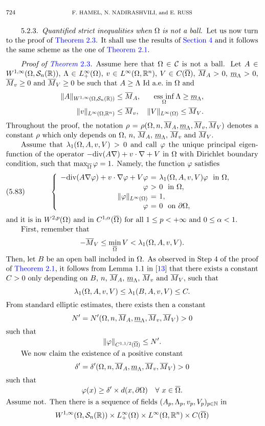
724 F. HAMEL, N. NADIRASHVILI, and E. RUSS
5.2.3. Quantified strict inequalities when Ω is not a ball. Let us now turn
to the proof of Theorem 2.3. It shall use the results of Section 4 and it follows
the same scheme as the one of Theorem 2.1.
Proof of Theorem 2.3. Assume here that Ω ∈ C is not a ball. Let A ∈W 1,∞(Ω,Sn(R)), Λ ∈ L∞+ (Ω), v ∈ L∞(Ω,Rn), V ∈ C(Ω), MA > 0, mΛ > 0,
Mv ≥ 0 and MV ≥ 0 be such that A ≥ Λ Id a.e. in Ω and
‖A‖W 1,∞(Ω,Sn(R)) ≤MA, ess infΩ
Λ ≥ mΛ,
‖v‖L∞(Ω,Rn) ≤Mv, ‖V ‖L∞(Ω) ≤MV .
Throughout the proof, the notation ρ = ρ(Ω, n,MA,mΛ,Mv,MV ) denotes a
constant ρ which only depends on Ω, n, MA, mΛ, Mv and MV .
Assume that λ1(Ω, A, v, V ) > 0 and call ϕ the unique principal eigen-
function of the operator −div(A∇) + v · ∇+ V in Ω with Dirichlet boundary
condition, such that maxΩ ϕ = 1. Namely, the function ϕ satisfies
(5.83)
−div(A∇ϕ) + v · ∇ϕ+ V ϕ = λ1(Ω, A, v, V )ϕ in Ω,
ϕ > 0 in Ω,
‖ϕ‖L∞(Ω) = 1,
ϕ = 0 on ∂Ω,
and it is in W 2,p(Ω) and in C1,α(Ω) for all 1 ≤ p < +∞ and 0 ≤ α < 1.
First, remember that
−MV ≤ minΩV < λ1(Ω, A, v, V ).
Then, let B be an open ball included in Ω. As observed in Step 4 of the proof
of Theorem 2.1, it follows from Lemma 1.1 in [13] that there exists a constant
C > 0 only depending on B, n, MA, mΛ, Mv and MV , such that
λ1(Ω, A, v, V ) ≤ λ1(B,A, v, V ) ≤ C.
From standard elliptic estimates, there exists then a constant
N ′ = N ′(Ω, n,MA,mΛ,Mv,MV ) > 0
such that
‖ϕ‖C1,1/2(Ω) ≤ N′.
We now claim the existence of a positive constant
δ′ = δ′(Ω, n,MA,mΛ,Mv,MV ) > 0
such that
ϕ(x) ≥ δ′ × d(x, ∂Ω) ∀ x ∈ Ω.
Assume not. Then there is a sequence of fields (Ap,Λp, vp, Vp)p∈N in
W 1,∞(Ω,Sn(R))× L∞+ (Ω)× L∞(Ω,Rn)× C(Ω)
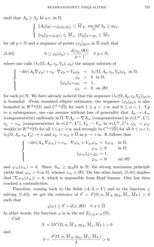
REARRANGEMENT INEQUALITIES 725
such that Ap ≥ Λp Id a.e. in Ω, ‖Ap‖W 1,∞(Ω,Sn(R)) ≤MA, ess infΩ
Λp ≥ mΛ,
‖vp‖L∞(Ω,Rn) ≤Mv, ‖Vp‖L∞(Ω) ≤MV
for all p ∈ N and a sequence of points (xp)p∈N in Ω such that
(5.84) 0 ≤ ϕp(xp) <d(xp, ∂Ω)
p+ 1∀ p ∈ N,
where one calls (λ1(Ω, Ap, vp, Vp), ϕp) the unique solution of−div(Ap∇ϕp) + vp · ∇ϕp + Vpϕp = λ1(Ω, Ap, vp, Vp)ϕp in Ω,
ϕp > 0 in Ω,
‖ϕp‖L∞(Ω) = 1,
ϕp = 0 on ∂Ω
for each p∈N. We have already noticed that the sequence (λ1(Ω,Ap,vp,Vp))p∈Nis bounded. From standard elliptic estimates, the sequence (ϕp)p∈N is also
bounded in W 2,q(Ω) and C1,α(Ω) for each 1 ≤ q < +∞ and 0 ≤ α < 1. Up
to a subsequence, one can assume without loss of generality that Ap → A∞(componentwise) uniformly in Ω, ∇Ap ∇A∞ (componentwise) in σ(L∞, L1),
vp v∞ (componentwise) in σ(L∞, L1), Vp V∞ in σ(L∞, L1), ϕp → ϕ∞weakly in W 2,q(Ω) for all 1≤q<+∞ and strongly in C1,α(Ω) for all 0 ≤ α<1,
λ1(Ω, Ap, vp, Vp)→ λ and xp → x∞ ∈ Ω as p→ +∞. It follows that−div(A∞∇ϕ∞) + v∞ · ∇ϕ∞ + V∞ϕ∞ = λϕ∞ in Ω,
ϕ∞ ≥ 0 in Ω,
‖ϕ∞‖L∞(Ω) = 1,
ϕ∞ = 0 on ∂Ω
and ϕ∞(x∞) = 0. Since A∞ ≥ mΛId in Ω, the strong maximum principle
yields that ϕ∞ > 0 in Ω, whence x∞ ∈ ∂Ω. On the other hand, (5.84) implies
that |∇ϕ∞(x∞)| = 0, which is impossible from Hopf lemma. One has then
reached a contradiction.
Therefore, coming back to the fields (A,Λ, v, V ) and to the function ϕ
solving (5.83), we get the existence of δ′ = δ′(Ω, n,MA,mΛ,Mv,MV ) > 0
such that
ϕ(x) ≥ δ′ × d(x, ∂Ω) ∀ x ∈ Ω.
In other words, the function ϕ is in the set E1/2,N ′,δ′(Ω).
Call
N = 3N ′(Ω, n,MA,mΛ,Mv,MV ) > 0
and
δ =δ′(Ω, n,MA,mΛ,Mv,MV )
3> 0.
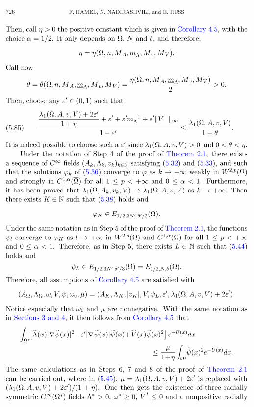
726 F. HAMEL, N. NADIRASHVILI, and E. RUSS
Then, call η > 0 the positive constant which is given in Corollary 4.5, with the
choice α = 1/2. It only depends on Ω, N and δ, and therefore,
η = η(Ω, n,MA,mΛ,Mv,MV ).
Call now
θ = θ(Ω, n,MA,mΛ,Mv,MV ) =η(Ω, n,MA,mΛ,Mv,MV )
2> 0.
Then, choose any ε′ ∈ (0, 1) such that
(5.85)
λ1(Ω, A, v, V ) + 2ε′
1 + η+ ε′ + ε′m−1
Λ + ε′‖V −‖∞
1− ε′≤ λ1(Ω, A, v, V )
1 + θ.
It is indeed possible to choose such a ε′ since λ1(Ω, A, v, V ) > 0 and 0 < θ < η.
Under the notation of Step 4 of the proof of Theorem 2.1, there exists
a sequence of C∞ fields (Ak,Λk, vk)k∈N satisfying (5.32) and (5.33), and such
that the solutions ϕk of (5.36) converge to ϕ as k → +∞ weakly in W 2,p(Ω)
and strongly in C1,α(Ω) for all 1 ≤ p < +∞ and 0 ≤ α < 1. Furthermore,
it has been proved that λ1(Ω, Ak, vk, V ) → λ1(Ω, A, v, V ) as k → +∞. Then
there exists K ∈ N such that (5.38) holds and
ϕK ∈ E1/2,2N ′,δ′/2(Ω).
Under the same notation as in Step 5 of the proof of Theorem 2.1, the functions
ψl converge to ϕK as l → +∞ in W 2,p(Ω) and C1,α(Ω) for all 1 ≤ p < +∞and 0 ≤ α < 1. Therefore, as in Step 5, there exists L ∈ N such that (5.44)
holds and
ψL ∈ E1/2,3N ′,δ′/3(Ω) = E1/2,N,δ(Ω).
Therefore, all assumptions of Corollary 4.5 are satisfied with
(AΩ,ΛΩ, ω, V, ψ, ω0, µ) = (AK ,ΛK , |vK |, V, ψL, ε′, λ1(Ω, A, v, V ) + 2ε′).
Notice especially that ω0 and µ are nonnegative. With the same notation as
in Sections 3 and 4, it then follows from Corollary 4.5 that∫Ω∗
îΛ(x)|∇ψ(x)|2−ε′|∇ψ(x)|ψ(x)+“V (x)ψ(x)2
óe−U(x)dx
≤ µ
1+η
∫Ω∗ψ(x)2e−U(x)dx.
The same calculations as in Steps 6, 7 and 8 of the proof of Theorem 2.1
can be carried out, where in (5.45), µ = λ1(Ω, A, v, V ) + 2ε′ is replaced with
(λ1(Ω, A, v, V ) + 2ε′)/(1 + η). One then gets the existence of three radially
symmetric C∞(Ω∗) fields Λ∗ > 0, ω∗ ≥ 0, V∗ ≤ 0 and a nonpositive radially
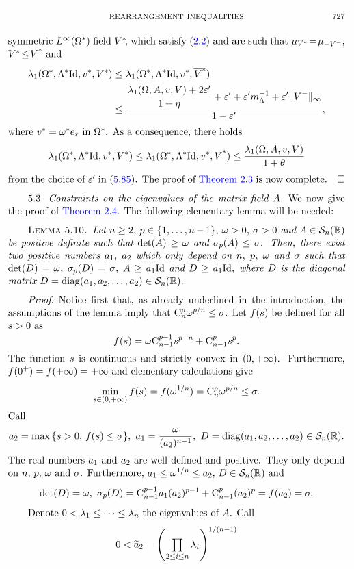
REARRANGEMENT INEQUALITIES 727
symmetric L∞(Ω∗) field V ∗, which satisfy (2.2) and are such that µV ∗=µ−V − ,
V ∗≤V ∗ and
λ1(Ω∗,Λ∗Id, v∗, V ∗) ≤ λ1(Ω∗,Λ∗Id, v∗, V∗)
≤
λ1(Ω, A, v, V ) + 2ε′
1 + η+ ε′ + ε′m−1
Λ + ε′‖V −‖∞
1− ε′,
where v∗ = ω∗er in Ω∗. As a consequence, there holds
λ1(Ω∗,Λ∗Id, v∗, V ∗) ≤ λ1(Ω∗,Λ∗Id, v∗, V∗) ≤ λ1(Ω, A, v, V )
1 + θ
from the choice of ε′ in (5.85). The proof of Theorem 2.3 is now complete.
5.3. Constraints on the eigenvalues of the matrix field A. We now give
the proof of Theorem 2.4. The following elementary lemma will be needed:
Lemma 5.10. Let n ≥ 2, p ∈ 1, . . . , n− 1, ω > 0, σ > 0 and A ∈ Sn(R)
be positive definite such that det(A) ≥ ω and σp(A) ≤ σ. Then, there exist
two positive numbers a1, a2 which only depend on n, p, ω and σ such that
det(D) = ω, σp(D) = σ, A ≥ a1Id and D ≥ a1Id, where D is the diagonal
matrix D = diag(a1, a2, . . . , a2) ∈ Sn(R).
Proof. Notice first that, as already underlined in the introduction, the
assumptions of the lemma imply that Cpnω
p/n ≤ σ. Let f(s) be defined for all
s > 0 as
f(s) = ωCp−1n−1s
p−n + Cpn−1s
p.
The function s is continuous and strictly convex in (0,+∞). Furthermore,
f(0+) = f(+∞) = +∞ and elementary calculations give
mins∈(0,+∞)
f(s) = f(ω1/n) = Cpnω
p/n ≤ σ.
Call
a2 = max s > 0, f(s) ≤ σ, a1 =ω
(a2)n−1, D = diag(a1, a2, . . . , a2) ∈ Sn(R).
The real numbers a1 and a2 are well defined and positive. They only depend
on n, p, ω and σ. Furthermore, a1 ≤ ω1/n ≤ a2, D ∈ Sn(R) and
det(D) = ω, σp(D) = Cp−1n−1a1(a2)p−1 + Cp
n−1(a2)p = f(a2) = σ.
Denote 0 < λ1 ≤ · · · ≤ λn the eigenvalues of A. Call
0 < a2 =
Ñ ∏2≤i≤n
λi
é1/(n−1)
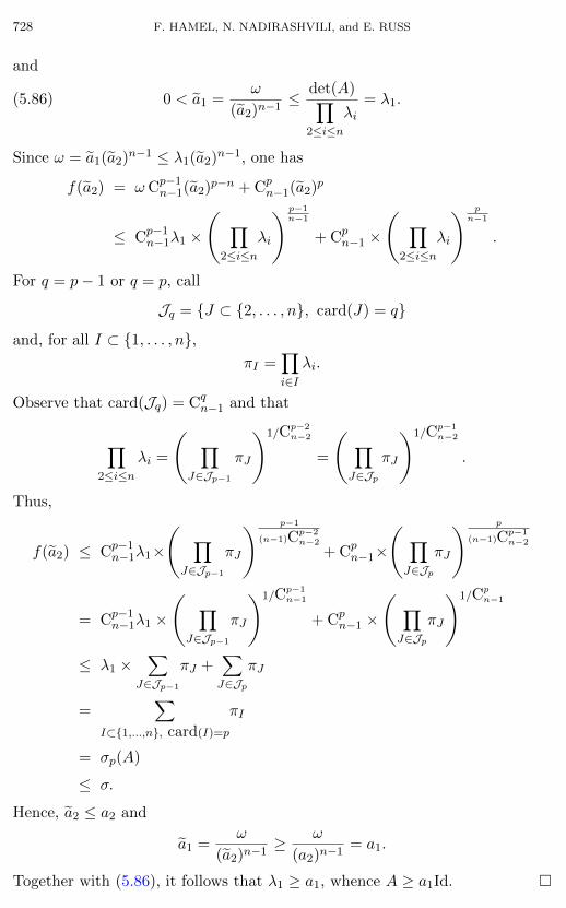
728 F. HAMEL, N. NADIRASHVILI, and E. RUSS
and
(5.86) 0 < a1 =ω
(a2)n−1≤ det(A)∏
2≤i≤nλi
= λ1.
Since ω = a1(a2)n−1 ≤ λ1(a2)n−1, one has
f(a2) = ωCp−1n−1(a2)p−n + Cp
n−1(a2)p
≤ Cp−1n−1λ1 ×
Ñ ∏2≤i≤n
λi
é p−1n−1
+ Cpn−1 ×
Ñ ∏2≤i≤n
λi
é pn−1
.
For q = p− 1 or q = p, call
Jq = J ⊂ 2, . . . , n, card(J) = q
and, for all I ⊂ 1, . . . , n,πI =
∏i∈I
λi.
Observe that card(Jq) = Cqn−1 and that
∏2≤i≤n
λi =
Ñ ∏J∈Jp−1
πJ
é1/Cp−2n−2
=
Ñ ∏J∈Jp
πJ
é1/Cp−1n−2
.
Thus,
f(a2) ≤ Cp−1n−1λ1×
Ñ ∏J∈Jp−1
πJ
é p−1
(n−1)Cp−2n−2
+ Cpn−1×
Ñ ∏J∈Jp
πJ
é p
(n−1)Cp−1n−2
= Cp−1n−1λ1 ×
Ñ ∏J∈Jp−1
πJ
é1/Cp−1n−1
+ Cpn−1 ×
Ñ ∏J∈Jp
πJ
é1/Cpn−1
≤ λ1 ×∑
J∈Jp−1
πJ +∑J∈Jp
πJ
=∑
I⊂1,...,n, card(I)=p
πI
= σp(A)
≤ σ.
Hence, a2 ≤ a2 and
a1 =ω
(a2)n−1≥ ω
(a2)n−1= a1.
Together with (5.86), it follows that λ1 ≥ a1, whence A ≥ a1Id.
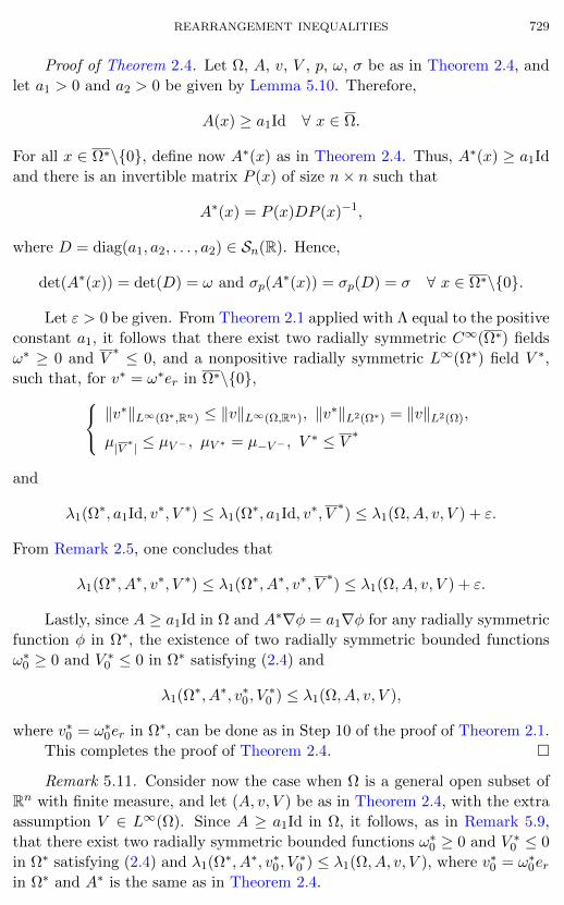
REARRANGEMENT INEQUALITIES 729
Proof of Theorem 2.4. Let Ω, A, v, V , p, ω, σ be as in Theorem 2.4, and
let a1 > 0 and a2 > 0 be given by Lemma 5.10. Therefore,
A(x) ≥ a1Id ∀ x ∈ Ω.
For all x ∈ Ω∗\0, define now A∗(x) as in Theorem 2.4. Thus, A∗(x) ≥ a1Id
and there is an invertible matrix P (x) of size n× n such that
A∗(x) = P (x)DP (x)−1,
where D = diag(a1, a2, . . . , a2) ∈ Sn(R). Hence,
det(A∗(x)) = det(D) = ω and σp(A∗(x)) = σp(D) = σ ∀ x ∈ Ω∗\0.
Let ε > 0 be given. From Theorem 2.1 applied with Λ equal to the positive
constant a1, it follows that there exist two radially symmetric C∞(Ω∗) fields
ω∗ ≥ 0 and V∗ ≤ 0, and a nonpositive radially symmetric L∞(Ω∗) field V ∗,
such that, for v∗ = ω∗er in Ω∗\0, ‖v∗‖L∞(Ω∗,Rn) ≤ ‖v‖L∞(Ω,Rn), ‖v∗‖L2(Ω∗) = ‖v‖L2(Ω),
µ|V ∗| ≤ µV − , µV ∗ = µ−V − , V∗ ≤ V ∗
and
λ1(Ω∗, a1Id, v∗, V ∗) ≤ λ1(Ω∗, a1Id, v∗, V∗) ≤ λ1(Ω, A, v, V ) + ε.
From Remark 2.5, one concludes that
λ1(Ω∗, A∗, v∗, V ∗) ≤ λ1(Ω∗, A∗, v∗, V∗) ≤ λ1(Ω, A, v, V ) + ε.
Lastly, since A ≥ a1Id in Ω and A∗∇φ = a1∇φ for any radially symmetric
function φ in Ω∗, the existence of two radially symmetric bounded functions
ω∗0 ≥ 0 and V ∗0 ≤ 0 in Ω∗ satisfying (2.4) and
λ1(Ω∗, A∗, v∗0, V∗
0 ) ≤ λ1(Ω, A, v, V ),
where v∗0 = ω∗0er in Ω∗, can be done as in Step 10 of the proof of Theorem 2.1.
This completes the proof of Theorem 2.4.
Remark 5.11. Consider now the case when Ω is a general open subset of
Rn with finite measure, and let (A, v, V ) be as in Theorem 2.4, with the extra
assumption V ∈ L∞(Ω). Since A ≥ a1Id in Ω, it follows, as in Remark 5.9,
that there exist two radially symmetric bounded functions ω∗0 ≥ 0 and V ∗0 ≤ 0
in Ω∗ satisfying (2.4) and λ1(Ω∗, A∗, v∗0, V∗
0 ) ≤ λ1(Ω, A, v, V ), where v∗0 = ω∗0erin Ω∗ and A∗ is the same as in Theorem 2.4.
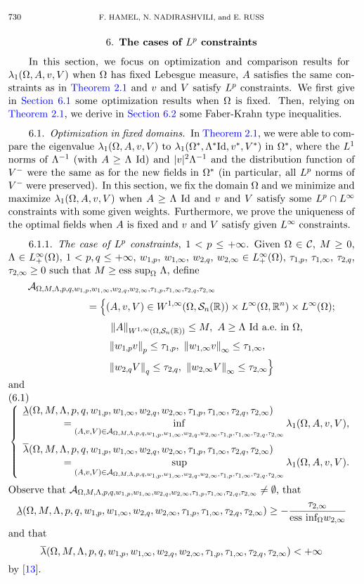
730 F. HAMEL, N. NADIRASHVILI, and E. RUSS
6. The cases of Lp constraints
In this section, we focus on optimization and comparison results for
λ1(Ω, A, v, V ) when Ω has fixed Lebesgue measure, A satisfies the same con-
straints as in Theorem 2.1 and v and V satisfy Lp constraints. We first give
in Section 6.1 some optimization results when Ω is fixed. Then, relying on
Theorem 2.1, we derive in Section 6.2 some Faber-Krahn type inequalities.
6.1. Optimization in fixed domains. In Theorem 2.1, we were able to com-
pare the eigenvalue λ1(Ω, A, v, V ) to λ1(Ω∗,Λ∗Id, v∗, V ∗) in Ω∗, where the L1
norms of Λ−1 (with A ≥ Λ Id) and |v|2Λ−1 and the distribution function of
V − were the same as for the new fields in Ω∗ (in particular, all Lp norms of
V − were preserved). In this section, we fix the domain Ω and we minimize and
maximize λ1(Ω, A, v, V ) when A ≥ Λ Id and v and V satisfy some Lp ∩ L∞constraints with some given weights. Furthermore, we prove the uniqueness of
the optimal fields when A is fixed and v and V satisfy given L∞ constraints.
6.1.1. The case of Lp constraints, 1 < p ≤ +∞. Given Ω ∈ C, M ≥ 0,
Λ ∈ L∞+ (Ω), 1 < p, q ≤ +∞, w1,p, w1,∞, w2,q, w2,∞ ∈ L∞+ (Ω), τ1,p, τ1,∞, τ2,q,
τ2,∞ ≥ 0 such that M ≥ ess supΩ Λ, define
AΩ,M,Λ,p,q,w1,p,w1,∞,w2,q ,w2,∞,τ1,p,τ1,∞,τ2,q ,τ2,∞
=
(A, v, V ) ∈W 1,∞(Ω,Sn(R))× L∞(Ω,Rn)× L∞(Ω);
‖A‖W 1,∞(Ω,Sn(R)) ≤M, A ≥ Λ Id a.e. in Ω,
‖w1,pv‖p ≤ τ1,p, ‖w1,∞v‖∞ ≤ τ1,∞,
‖w2,qV ‖q ≤ τ2,q, ‖w2,∞V ‖∞ ≤ τ2,∞
and
(6.1)
λ(Ω,M,Λ, p, q, w1,p, w1,∞, w2,q, w2,∞, τ1,p, τ1,∞, τ2,q, τ2,∞)
= inf(A,v,V )∈AΩ,M,Λ,p,q,w1,p,w1,∞,w2,q,w2,∞,τ1,p,τ1,∞,τ2,q,τ2,∞
λ1(Ω, A, v, V ),
λ(Ω,M,Λ, p, q, w1,p, w1,∞, w2,q, w2,∞, τ1,p, τ1,∞, τ2,q, τ2,∞)
= sup(A,v,V )∈AΩ,M,Λ,p,q,w1,p,w1,∞,w2,q,w2,∞,τ1,p,τ1,∞,τ2,q,τ2,∞
λ1(Ω, A, v, V ).
Observe that AΩ,M,Λ,p,q,w1,p,w1,∞,w2,q ,w2,∞,τ1,p,τ1,∞,τ2,q ,τ2,∞ 6= ∅, that
λ(Ω,M,Λ, p, q, w1,p, w1,∞, w2,q, w2,∞, τ1,p, τ1,∞, τ2,q, τ2,∞) ≥ − τ2,∞ess infΩw2,∞
and that
λ(Ω,M,Λ, p, q, w1,p, w1,∞, w2,q, w2,∞, τ1,p, τ1,∞, τ2,q, τ2,∞) < +∞
by [13].
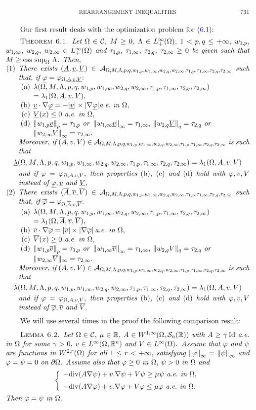
REARRANGEMENT INEQUALITIES 731
Our first result deals with the optimization problem for (6.1):
Theorem 6.1. Let Ω ∈ C, M ≥ 0, Λ ∈ L∞+ (Ω), 1 < p, q ≤ +∞, w1,p,
w1,∞, w2,q , w2,∞ ∈ L∞+ (Ω) and τ1,p, τ1,∞, τ2,q , τ2,∞ ≥ 0 be given such that
M ≥ ess supΩ Λ. Then,(1) There exists (A, v, V ) ∈ AΩ,M,Λ,p,q,w1,p,w1,∞,w2,q ,w2,∞,τ1,p,τ1,∞,τ2,q ,τ2,∞ such
that, if ϕ = ϕΩ,A,v,V :
(a) λ(Ω,M,Λ, p, q, w1,p, w1,∞, w2,q, w2,∞, τ1,p, τ1,∞, τ2,q, τ2,∞)
= λ1(Ω, A, v, V ),
(b) v · ∇ϕ = −|v| × |∇ϕ|a.e. in Ω,
(c) V (x) ≤ 0 a.e. in Ω,
(d) ‖w1,pv‖p = τ1,p or ‖w1,∞v‖∞ = τ1,∞, ‖w2,qV ‖q = τ2,q or
‖w2,∞V ‖∞ = τ2,∞.
Moreover, if (A, v, V ) ∈ AΩ,M,Λ,p,q,w1,p,w1,∞,w2,q ,w2,∞,τ1,p,τ1,∞,τ2,q ,τ2,∞ is such
that
λ(Ω,M,Λ, p, q, w1,p, w1,∞, w2,q, w2,∞, τ1,p, τ1,∞, τ2,q, τ2,∞) = λ1(Ω, A, v, V )
and if ϕ = ϕΩ,A,v,V , then properties (b), (c) and (d) hold with ϕ, v, V
instead of ϕ, v and V ,
(2) There exists (A, v, V ) ∈ AΩ,M,Λ,p,q,w1,p,w1,∞,w2,q ,w2,∞,τ1,p,τ1,∞,τ2,q ,τ2,∞ such
that, if ϕ = ϕΩ,A,v,V :
(a) λ(Ω,M,Λ, p, q, w1,p, w1,∞, w2,q, w2,∞, τ1,p, τ1,∞, τ2,q, τ2,∞)
= λ1(Ω, A, v, V ),
(b) v · ∇ϕ = |v| × |∇ϕ| a.e. in Ω,
(c) V (x) ≥ 0 a.e. in Ω,
(d) ‖w1,pv‖p = τ1,p or ‖w1,∞v‖∞ = τ1,∞, ‖w2,qV ‖q = τ2,q or
‖w2,∞V ‖∞ = τ2,∞.
Moreover, if (A, v, V ) ∈ AΩ,M,Λ,p,q,w1,p,w1,∞,w2,q ,w2,∞,τ1,p,τ1,∞,τ2,q ,τ2,∞ is such
that
λ(Ω,M,Λ, p, q, w1,p, w1,∞, w2,q, w2,∞, τ1,p, τ1,∞, τ2,q, τ2,∞) = λ1(Ω, A, v, V )
and if ϕ = ϕΩ,A,v,V , then properties (b), (c) and (d) hold with ϕ, v, V
instead of ϕ, v and V .
We will use several times in the proof the following comparison result:
Lemma 6.2. Let Ω ∈ C, µ ∈ R, A ∈ W 1,∞(Ω,Sn(R)) with A ≥ γ Id a.e.
in Ω for some γ > 0, v ∈ L∞(Ω,Rn) and V ∈ L∞(Ω). Assume that ϕ and ψ
are functions in W 2,r(Ω) for all 1 ≤ r < +∞, satisfying ‖ϕ‖∞ = ‖ψ‖∞ and
ϕ = ψ = 0 on ∂Ω. Assume also that ϕ ≥ 0 in Ω, ψ > 0 in Ω and−div(A∇ψ) + v.∇ψ + V ψ ≥ µψ a.e. in Ω,
−div(A∇ϕ) + v.∇ϕ+ V ϕ ≤ µϕ a.e. in Ω.
Then ϕ = ψ in Ω.
732 F. HAMEL, N. NADIRASHVILI, and E. RUSS
Proof. The proof uses a classical comparison method. (This method was
used for instance in [13].) We give it here for the sake of completeness. Since
ψ > 0 in Ω and ψ = 0 on ∂Ω, the Hopf lemma yields ν(x) · ∇ψ(x) < 0 on ∂Ω,
where, for all x ∈ ∂Ω, ν(x) denotes the outward normal unit vector at x. Since
ϕ ∈ C1,β(Ω) for all 0 ≤ β < 1, ϕ ≥ 0 in Ω and ϕ = 0 on ∂Ω, it follows that
there exists γ > 0 such that γψ > ϕ in Ω. Define
γ∗ = inf γ > 0, γψ > ϕ in Ω .
One clearly has γ∗ψ ≥ ϕ in Ω, so that γ∗ > 0. Define w = γ∗ψ − ϕ ≥ 0 and
assume that w > 0 everywhere in Ω. Since
(6.2) − div(A∇w) + v · ∇w + V w − µw ≥ 0 a.e. in Ω
and w = 0 on ∂Ω, the Hopf maximum principle implies that ν ·∇w < 0 on ∂Ω.
As above, this yields the existence of κ > 0 such that w > κϕ in Ω, whence
γ∗ψ/(1+κ) > ϕ in Ω. This is a contradiction with the minimality of γ∗. Thus,
there exists x0 ∈ Ω such that w(x0) = 0 (i.e. γ∗ψ(x0) = ϕ(x0)). Since w ≥ 0
in Ω, it follows from (6.2) and from the strong maximum principle, that w = 0
in Ω, which means that ϕ and ψ are proportional. Since they are nonnegative
in Ω and have the same L∞ norm in Ω, one has ϕ = ψ, which ends the proof
of Lemma 6.2.
For the proof of Theorem 6.1, we will treat the minimization problem only,
the maximization problem being clearly analogous. It is plain to see that the
result is a consequence of the two following lemmata:
Lemma 6.3. Let Ω ∈ C, M ≥ 0, Λ ∈ L∞+ (Ω), 1 < p, q ≤ +∞, w1,p,
w1,∞, w2,q , w2,∞ ∈ L∞+ (Ω) and τ1,p, τ1,∞, τ2,q , τ2,∞ ≥ 0 be given such that
M ≥ ess supΩ Λ. Assume that
(A, v, V ) ∈ AΩ,M,Λ,p,q,w1,p,w1,∞,w2,q ,w2,∞,τ1,p,τ1,∞,τ2,q ,τ2,∞
is such that
(6.3)
λ(Ω,M,Λ, p, q, w1,p, w1,∞, w2,q, w2,∞, τ1,p, τ1,∞, τ2,q, τ2,∞) = λ1(Ω, A, v, V ),
and let ϕ = ϕΩ,A,v,V . Then, properties (b), (c) and (d) in Theorem 6.1 hold.
Lemma 6.4. Let Ω ∈ C, M ≥ 0, Λ ∈ L∞+ (Ω), 1 < p, q ≤ +∞, w1,p,
w1,∞, w2,q , w2,∞ ∈ L∞+ (Ω) and τ1,p, τ1,∞, τ2,q , τ2,∞ ≥ 0 be given such that
M ≥ ess supΩ Λ. Then, there exists
(A, v, V ) ∈ AΩ,M,Λ,p,q,w1,p,w1,∞,w2,q ,w2,∞,τ1,p,τ1,∞,τ2,q ,τ2,∞
such that (6.3) holds.
REARRANGEMENT INEQUALITIES 733
Proof of Lemma 6.3. Let A, v, V and ϕ as in Lemma 6.3. Remember that
ϕ ∈ C1(Ω). Define, for a.e. x ∈ Ω,
w(x) =
− |v(x)|
∇ϕ(x)∣∣∣∇ϕ(x)∣∣∣ if ∇ϕ(x) 6= 0,
0 if ∇ϕ(x) = 0
so that w · ∇ϕ = − |v| ×∣∣∣∇ϕ∣∣∣ ≤ v · ∇ϕ a.e. in Ω, and set
µ = λ1(Ω, A, w, V ) and ψ = ϕΩ,A,w,V .
Notice that |w| ≤ |v| a.e. in Ω, whence
(A,w, V ) ∈ AΩ,M,Λ,p,q,w1,p,w1,∞,w2,q ,w2,∞,τ1,p,τ1,∞,τ2,q ,τ2,∞
and
λ := λ(Ω,M,Λ, p, q, w1,p, w1,∞, w2,q, w2,∞, τ1,p, τ1,∞, τ2,q, τ2,∞) ≤ µ.
Thus, one has−div(A∇ϕ) + w·∇ϕ+ V ϕ ≤ −div(A∇ϕ) + v ·∇ϕ+ V ϕ = λϕ ≤ µϕ
−div(A∇ψ) + w·∇ψ + V ψ = µψ
a.e. in Ω, and Lemma 6.2 yields ψ = ϕ and therefore µ = λ and v · ∇ϕ =
w · ∇ϕ = − |v| ×∣∣∣∇ϕ∣∣∣ a.e. in Ω.
As far as assertion (c) is concerned, define, for a.e. x ∈ Ω,
W (x) =
V (x) if V (x) ≤ 0,
0 if V (x) > 0.
Observe that |W | ≤ |V | a.e. in Ω, whence
(A, v,W ) ∈ AΩ,M,Λ,p,q,w1,p,w1,∞,w2,q ,w2,∞,τ1,p,τ1,∞,τ2,q ,τ2,∞ .
If µ = λ1(Ω, A, v,W ) and ψ = ϕΩ,A,v,W , one therefore has λ ≤ µ and
−div(A∇ψ) + v · ∇ψ +Wψ = µψ a.e. in Ω,
while, since Wϕ ≤ V ϕ a.e. in Ω,
−div(A∇ϕ) + v · ∇ϕ+Wϕ ≤ µϕ a.e. in Ω.
Lemma 6.2 therefore shows that ψ = ϕ, and it follows that Wϕ = V ϕ a.e. in
Ω, which implies W = V a.e. in Ω since ϕ > 0 in Ω, and this is assertion (c).
Assume now that ‖w1,pv‖p < τ1,p and ‖w1,∞v‖∞ < τ1,∞, and define, for
a.e. x ∈ Ω,
w(x) =
− (|v(x)|+ ε)
∇ϕ(x)∣∣∣∇ϕ(x)∣∣∣ if ∇ϕ(x) 6= 0,
0 if ∇ϕ(x) = 0,
734 F. HAMEL, N. NADIRASHVILI, and E. RUSS
where ε > 0 is choosen in such a way that ‖w1,pw‖p ≤ τ1,p and ‖w1,∞w‖∞ ≤τ1,∞, so that, if µ = λ1(Ω, A, w, V ), one has λ ≤ µ. Let ψ = ϕΩ,A,w,V . Observe
that
−div(A∇ϕ) + w · ∇ϕ+ V ϕ ≤ λϕ ≤ µϕ a.e. in Ω,
since w · ∇ϕ = − (|v|+ ε)∣∣∣∇ϕ∣∣∣ ≤ −|v| × |∇ϕ| ≤ v · ∇ϕ a.e. in Ω, while
−div(A∇ψ) + w · ∇ψ + V ψ = µψ a.e. in Ω.
Another application of Lemma 6.2 yields that ψ = ϕ and therefore w · ∇ϕ =
v ·∇ϕ, so that −ε∣∣∣∇ϕ∣∣∣ = 0 a.e. in Ω, which is impossible. One argues similarly
for V , using the fact that V ≤ 0 a.e. in Ω.
Proof of Lemma 6.4. Write
λ = λ(Ω,M,Λ, p, q, w1,p, w1,∞, w2,q, w2,∞, τ1,p, τ1,∞, τ2,q, τ2,∞).
There exist a sequence (Ak)k∈N ∈ W 1,∞(Ω,Sn(R)) with ‖Ak‖W 1,∞(Ω,Sn(R))
≤M and Ak ≥ Λ Id a.e. in Ω, a sequence (vk)k∈N ∈ L∞(Ω,Rn) with ‖w1,pvk‖p≤ τ1,p and ‖w1,∞vk‖∞ ≤ τ1,∞, and a sequence (Vk)k∈N ∈ L∞(Ω) with ‖w2,qVk‖q≤ τ2,q and ‖w2,∞Vk‖∞ ≤ τ2,∞, such that
λk := λ1(Ω, Ak, vk, Vk)→ λ as k → +∞.
For each k ∈ N, call ϕk = ϕΩ,Ak,vk,Vk , so that
−div(Ak∇ϕk) + vk · ∇ϕk + Vkϕk = λkϕk in Ω and ϕk = 0 on ∂Ω.
By the usual elliptic estimates, the functions ϕk’s are uniformly bounded in the
spaces W 2,r(Ω) for all 1 ≤ r < +∞, and therefore in C1,α(Ω) for all 0 ≤ α < 1.
Therefore, up to a subsequence, one may assume that, for some nonnegative
function ϕ ∈ W 2,r(Ω) for all 1 ≤ r < +∞, ϕk ϕ weakly in W 2,r(Ω)
for all 1 ≤ r < +∞ and ϕk → ϕ strongly in C1,α(Ω) for all 0 ≤ α < 1,
as k → +∞. Similarly, there exists A ∈ W 1,∞(Ω,Sn(R)) such that (up to
extraction), Ak → A uniformly in Ω and, for each 1 ≤ j ≤ n, ∂jAk ∂jA
in σ(L∞(Ω), L1(Ω)) componentwise. In particular, ‖A‖W 1,∞(Ω,Sn(R)) ≤M and
A ≥ Λ Id a.e. in Ω. Finally, up to extraction again, there exists ω ∈ L∞(Ω)
such that |vk| ω ≥ 0 in L∞(Ω) weak-* and then weakly in Lr(Ω) for all
1 ≤ r < +∞, and there exists V ∈ L∞(Ω) such that Vk V in L∞(Ω)
weak-* and then weakly in Lr(Ω) for all 1 ≤ r < +∞. Since, for all k ≥ 1, by
Cauchy-Schwarz,
−div(Ak∇ϕk)− |vk| |∇ϕk|+ Vkϕk ≤ λkϕk a.e. in Ω,
one has
−div(A∇ϕ)− ω∣∣∣∇ϕ∣∣∣+ V ϕ ≤ λϕ a.e. in Ω.
REARRANGEMENT INEQUALITIES 735
Define now, for a.e. x ∈ Ω,
v(x) =
−ω(x)
∇ϕ(x)∣∣∣∇ϕ(x)∣∣∣ if ∇ϕ(x) 6= 0,
0 if ∇ϕ(x) = 0,
so that v · ∇ϕ = −ω∣∣∣∇ϕ∣∣∣ a.e. in Ω. One therefore has
(6.4) − div(A∇ϕ) + v · ∇ϕ+ V ϕ ≤ λϕ a.e. in Ω and ϕ = 0 on ∂Ω.
Observe that (A, v, V ) ∈ AΩ,M,Λ,p,q,w1,p,w1,∞,w2,q ,w2,∞,τ1,p,τ1,∞,τ2,q ,τ2,∞ . Define
now µ = λ1(Ω, A, v, V ) and ψ = ϕΩ,A,v,V , so that λ ≤ µ. It follows from (6.4)
that −div(A∇ψ) + v · ∇ψ + V ψ = µψ a.e. in Ω,
−div(A∇ϕ) + v · ∇ϕ+ V ϕ ≤ µϕ in Ω.
Moreover, ϕ ≥ 0 in Ω, ψ > 0 in Ω, ϕ = ψ = 0 on ∂Ω and∥∥∥ϕ∥∥∥
∞= ‖ψ‖∞ = 1.
Lemma 6.2 therefore yields ϕ = ψ, hence λ = µ. This ends the proof of
Lemma 6.4.
Remark 6.5. What happens in Theorem 6.1 if one drops the L∞ bounds
for v or V ? Even if one still assumes that v and V are qualitatively in L∞ (so
that the principal eigenvalue of −div(A∇) + v · ∇+ V is well defined by [13]),
it turns out that the infimum or the supremum considered there may not be
achieved. For instance, fix 1 < p < n, Ω ∈ C, τ > 0, A = Id and V = 0 in Ω,
and define
λ(Ω, τ) = infv∈L∞(Ω,Rn), ‖v‖p≤τ
λ1(Ω, Id, v, 0).
Since the operator −∆+v ·∇ satisfies the maximum principle in Ω, its principal
eigenvalue is positive, for each v ∈ L∞(Ω,Rn), and therefore λ(Ω, τ) ≥ 0. We
claim that λ(Ω, τ) = 0. Indeed, fix ρ0 > 0 such that there exists a ball B0
with radius ρ0 included in Ω. Call x0 its center. For all A > 0 large enough,
define ρA ∈ (0, ρ0) such that A(αnρnA)1/p = τ (recall that αn is the Lebesgue
measure of the Euclidean unit ball in Rn), let BA = B(x0, ρA) be the ball with
the same center x0 as B0 and with radius ρA, and set v = A×1BAer(·−x0) in
Ω, so that ‖v‖Lp(Ω,Rn) = τ . One has λ1(Ω, Id, v, 0) ≤ λ1(BA, Id, Aer(· − x0), 0)
since BA ⊂ Ω. But
λ1(BA, Id, Aer(· − x0), 0) =µAρ2A
,
where µA = λ1(‹B, Id, AρAer(· − x0), 0) is the principal eigenvalue of −∆ +
AρAer(· − x0) · ∇ on the ball ‹B with center x0 and with radius 1, under
Dirichlet boundary condition. Notice that AρA → +∞ as A → +∞ since
1 < p < n. Furthermore, µA = λ1(Bn1 , AρAer) under the notation (2.15),
where Bn1 is the Euclidean ball of Rn with center 0 and radius 1. It then
736 F. HAMEL, N. NADIRASHVILI, and E. RUSS
follows immediately from Appendix 7.3 that logµA ∼ −AρA when A → +∞(see also [22] for related results under stronger regularity assumptions). As a
consequence, there exists A0 > 0 such that, for all A > A0,
λ1(BA, Id, Aer(· − x0), 0) ≤ e−AρA/2
ρ2A
= α2/nn τ−2p/nA2p/ne−(α
−1/nn τp/nA1−p/n)/2,
and this expression goes to 0 when A→ +∞, which proves the claim.
Similarly, one can show that, if Ω ∈ C, τ > 0 and 1 < q < n/2 are fixed,
(6.5) infV ∈L∞(Ω); ‖V ‖q≤τ
λ1(Ω, Id, 0, V ) = −∞.
Indeed, fix ρ0 as before, and, for all A large enough, let ρA ∈ (0, ρ0) such that
AqαnρnA = τ q, and set V = −A × 1BA where BA = B(x0, ρA) is defined as
previously, so that ‖V ‖Lq(Ω) = τ . One has
λ1(Ω, Id, 0, V ) ≤ λ1(BA, Id, 0,−A) = λ1(BA, Id, 0, 0)−A
(6.6)
=C
ρ2A
−A = Cα2/nn τ−2q/nA2q/n −A,
where C = λ1(‹B, Id, 0, 0) > 0. The right-hand side of (6.6) goes to −∞ when
A→ +∞, due to the choice of q. This ends the proof of the claim (6.5).
6.1.2. The case of L∞ constraints. When solving optimization problems
for λ1(Ω, A, v, V ) if A is fixed and v, V vary and satisfy L∞ bounds, we can
precise the conclusions of Theorem 6.1. Fix Ω ∈ C and A ∈ W 1,∞(Ω,Sn(R))
such that A ≥ γ Id in Ω for some positive real number γ > 0. Given τ1, τ2 ≥ 0
and w1 ∈ L∞+ (Ω), define
AΩ,A,w1,τ1,τ2 = (v, V ) ∈ L∞(Ω,Rn)× L∞(Ω); ‖w1v‖∞ ≤ τ1, ‖V ‖∞ ≤ τ2, ,
and λ(Ω, A,w1, τ1, τ2) = inf
(v,V )∈AΩ,A,w1,τ1,τ2
λ1(Ω, A, v, V ),
λ(Ω, A,w1, τ1, τ2) = sup(v,V )∈AΩ,A,w1,τ1,τ2
λ1(Ω, A, v, V ).
The optimization results under these constraints are the following ones:
Theorem 6.6. Let Ω ∈ C, A ∈ W 1,∞(Ω,Sn(R)) such that A ≥ γId in Ω
for some γ > 0, τ1, τ2 ≥ 0 and w1 ∈ L∞+ (Ω) be given.Then :
(1) There exist a unique vector field v ∈ L∞(Ω,Rn) with ‖w1v‖∞ ≤ τ1 and a
unique function V ∈ L∞(Ω) with ‖V ‖∞ ≤ τ2, such that
λ(Ω, A,w1, τ1, τ2) = λ1(Ω, A, v, V ).
Moreover, if ϕ = ϕΩ,A,v,V , one has
REARRANGEMENT INEQUALITIES 737
(a) v · ∇ϕ = −τ1w−11
∣∣∣∇ϕ∣∣∣ a.e. in Ω,
(b) |v(x)|w1(x) = τ1 a.e. in Ω,
(c) V (x) = −τ2 a.e. in Ω.
Furthermore, ∇ϕ(x) 6= 0 a.e. in Ω and v(x) = −τ1w1(x)−1∇ϕ(x)/|∇ϕ(x)|a.e. in Ω.
(2) There exist a unique vector field v ∈ L∞(Ω,Rn) with ‖w1v‖∞ ≤ τ1 and a
unique function V ∈ L∞(Ω) with ‖V ‖∞ ≤ τ2, such that
λ(Ω, A,w1, τ1, τ2) = λ1(Ω, A, v, V ).
Moreover, if ϕ = ϕΩ,A,v,V , one has
(a) v · ∇ϕ = τ1w−11 |∇ϕ| a.e. in Ω,
(b) |v(x)|w1(x) = τ1 a.e. in Ω,
(c) V (x) = τ2 a.e. in Ω.
Furthermore, ∇ϕ(x) 6= 0 a.e. in Ω and v(x) = +τ1w1(x)−1∇ϕ(x)/|∇ϕ(x)|a.e. in Ω.
Proof. As in the proof of Theorem 6.1, let us focus on the minimization
problem. The existence of v and V such that λ1(Ω, A, v, V ) = λ(Ω, A,w1, τ1, τ2)
is obtained in the same way as in Lemma 6.4, except that one has to define,
for almost every x ∈ Ω,
v(x) =
−τ1w1(x)−1 ∇ϕ(x)∣∣∣∇ϕ(x)
∣∣∣ if ∇ϕ(x) 6= 0,
0 if ∇ϕ(x) = 0,
and V (x) = −τ2 for all x ∈ Ω, and that we do not need to introduce the vector
field w. To prove the uniqueness of V , proceed as in the proof of assertion (c)
in Lemma 6.3. We are now left with the task of proving the uniqueness of v
and the fact that w1(x) |v(x)| = τ1 for almost every x ∈ Ω.
First, arguing as in the proof of Lemma 6.3, one shows that, if v and
V are such that λ1(Ω, A, v, V ) = λ(Ω, A,w1, τ1, τ2) and if ϕ = ϕΩ,A,v,V , then
v · ∇ϕ = −τ1w−11 |∇ϕ| a.e. in Ω.
To conclude, we need the following lemma:
Lemma 6.7. Let λ ∈ R and ψ ∈ W 2,r(Ω) for all 1 ≤ r < +∞, be such
that ψ = 0 on ∂Ω, ψ > 0 in Ω, ‖ψ‖∞ = 1 and
−div(A∇ψ)− τ1w−11 |∇ψ| − τ2ψ = λψ in Ω.
Let v ∈ L∞(Ω,Rn) be such that ‖w1v‖∞ ≤ τ1 and
λ1(Ω, A, v,−τ2) = λ(Ω, A,w1, τ1, τ2).
Then λ = λ(Ω, A,w1, τ1, τ2) and ψ = ϕΩ,A,v,−τ2 .
738 F. HAMEL, N. NADIRASHVILI, and E. RUSS
Proof of Lemma 6.7. Let v be as above and set ϕ = ϕΩ,A,v,−τ2 , so that
−div(A∇ϕ)− τ1w−11 |∇ϕ| − τ2ϕ = −div(A∇ϕ) + v · ∇ϕ− τ2ϕ
= λ(Ω, A,w1, τ1, τ2)ϕ in Ω
by what we have just seen. Define also
w(x) =
−τ1w1(x)−1 ∇ψ(x)
|∇ψ(x)|if ∇ψ(x) 6= 0,
0 if ∇ψ(x) = 0.
One has ‖w1w‖∞ = τ1 and
−div(A∇ψ) + w·∇ψ − τ2ψ = −div(A∇ψ)− τ1w−11 |∇ψ| − τ2ψ = λψ in Ω,
so that, since ψ > 0 in Ω and ψ = 0 on ∂Ω, by the characterization of the prin-
cipal eigenfunction and the normalization ‖ψ‖∞ = 1, one has ψ = ϕΩ,A,w,−τ2and
λ = λ1(Ω, A,w,−τ2) ≥ λ(Ω, A,w1, τ1, τ2).
As a consequence,
−div(A∇ψ) + v · ∇ψ − τ2ψ ≥ −div(A∇ψ)− τ1w−11 |∇ψ| − τ2ψ
= λψ ≥ λ(Ω, A,w1, τ1, τ2)ψ in Ω,
while
−div(A∇ϕ) + v · ∇ϕ− τ2ϕ = λ1(Ω, A, v,−τ2)ϕ = λ(Ω, A,w1, τ1, τ2)ϕ in Ω
by assumption. Since ψ > 0 in Ω, another application of Lemma 6.2 shows
that ψ = ϕ = ϕΩ,A,v,−τ2 , and that λ = λ(Ω, A,w1, τ1, τ2).
With the help of Lemma 6.7, we conclude the proof of Theorem 6.6. Let
v1 ∈ L∞(Ω,Rn) and v2 ∈ L∞(Ω,Rn) with ‖w1v1‖∞ ≤ τ1 and ‖w1v2‖∞ ≤ τ1
be such that
λ(Ω, A,w1, τ1, τ2) = λ1(Ω, A, v1,−τ2) = λ1(Ω, A, v2,−τ2),
and set
ϕ1 = ϕΩ,A,v1,−τ2 and ϕ2 = ϕΩ,A,v2−τ2 .
Since v1 · ∇ϕ1 = −τ1w−11 |∇ϕ1| and v2 · ∇ϕ2 = −τ1w
−11 |∇ϕ2| a.e. in Ω, one
has −div(A∇ϕ1)− τ1w
−11 |∇ϕ1| − τ2ϕ1 = λ(Ω, A,w1, τ1, τ2)ϕ1 in Ω,
−div(A∇ϕ2)− τ1w−11 |∇ϕ2| − τ2ϕ2 = λ(Ω, A,w1, τ1, τ2)ϕ2 in Ω,
with ϕ1, ϕ2 ∈⋂
1≤r<+∞W2,r(Ω), ϕ1, ϕ2 > 0 in Ω, ‖ϕ1‖∞ = ‖ϕ2‖∞ = 1, and
ϕ1 = ϕ2 = 0 on ∂Ω. Lemma 6.7 shows that ϕ1 =ϕΩ,A,v2,−τ2 =ϕ2 :=ϕ, so that
v1 ·∇ϕ=v2 ·∇ϕ=−τ1w−11 |∇ϕ|. It follows that v1 = v2 and |v1| = |v2| = τ1w
−11
a.e. on the set x ∈ Ω; ∇ϕ(x) 6= 0. It remains to be observed that ∇ϕ(x) 6= 0
REARRANGEMENT INEQUALITIES 739
a.e. in Ω. Indeed, if E = x ∈ Ω; ∇ϕ(x) = 0, one has div(A∇ϕ) = 0 a.e. in
E, so that −τ2ϕ = λ1(Ω, A, v1,−τ2)ϕ in E, and since λ1(Ω, A, v1,−τ2) > −τ2,
one has |E| = 0.
If, in Theorem 6.6, we specialize to the case when Ω is a ball and the
diffusion matrix A is equal to Λ Id with Λ radially symmetric, we obtain
a more complete description of the unique minimizer and maximizer. More
precisely, we have:
Theorem 6.8. Assume that Ω is a Euclidean ball centered at 0 with radius
R > 0, let Λ ∈ L∞+ (Ω) ∩W 1,∞(Ω) be radially symmetric, set A = ΛId and use
the same notation as in Theorem 6.6, under the extra assumption that w1 is
radially symmetric Then, v = τ1w−11 er, v = −τ1w
−11 er a.e. in Ω, and ϕ and ϕ
are radially symmetric and decreasing.
Proof. Let ϕ = ϕ = ϕΩ,ΛId,v,−τ2 where v is given in Theorem 6.6. One
has
(6.7) − div(Λ∇ϕ)− τ1w−11 |∇ϕ| − τ2ϕ = λ(Ω, A,w1, τ1, τ2)ϕ
in Ω. If S is any orthogonal transformation in Rn and ψ = ϕ S, then
ψ ∈ W 2,r(Ω) for all 1 ≤ r < +∞, satisfies (6.7), vanishes on ∂Ω and is
positive in Ω. Lemma 6.7 therefore yields ϕ = ψ, which means that ϕ is
radially symmetric, so that there exists a function u : [0, R] → R such that
ϕ(x) = u (|x|) for all x ∈ Ω, and u is C1,α([0, R]) for all 0 ≤ α < 1. Let
0 ≤ r1 < r2 < R. Remind that λ(Ω, A,w1, τ1, τ2) = λ1(Ω, A, v,−τ2) > −τ2.
Since
(6.8) − div(Λ∇ϕ) + v · ∇ϕ = (λ(Ω, A,w1, τ1, τ2) + τ2)ϕ > 0
in Ω, the maximum principle applied to ϕ in Br2 yields that ϕ ≥ u(r2) in
Br2 , which means that u(r1) ≥ u(r2). Moreover, if u(r1) = u(r2), the strong
maximum principle implies that ϕ is constant in Br2 , which is impossible be-
cause of (6.8). Therefore, u(r1) > u(r2). Finally, if 0 ≤ r1 < r2 = R, one has
immediately u(r1) > u(r2) = 0. Thus, u is decreasing in [0, R], and this yields
at once v = τ1w−11 er from Theorem 6.6.
The arguments for ϕ and v are entirely analogous and this completes the
proof of Theorem 6.8.
6.2. Faber-Krahn inequalities.
Proof of Theorem 2.7. First, since ‖V ‖∞ ≤ τ2, it follows from [13] that
λ1(Ω, A, v, V ) ≥ λ1(Ω, A, v,−τ2) = −τ2 + λ1(Ω, A, v, 0).
But λ1(Ω, A, v, 0) > 0. Theorem 2.3 then yields the existence of a positive
constant θ = θ(Ω, n,MA,mΛ, τ1) > 0 depending only on (Ω, n,MA,mΛ, τ1),
740 F. HAMEL, N. NADIRASHVILI, and E. RUSS
and the existence of two radially symmetric C∞(Ω∗) fields Λ∗ > 0, ω∗ ≥ 0
such that, for v∗ = ω∗er in Ω∗,ess inf
ΩΛ ≤ min
Ω∗Λ∗ ≤ max
Ω∗Λ∗ ≤ ess sup
ΩΛ, ‖(Λ∗)−1‖L1(Ω∗) = ‖Λ−1‖L1(Ω),
‖v∗‖L∞(Ω∗,Rn)≤‖v‖L∞(Ω,Rn), ‖ |v∗|2(Λ∗)−1‖L1(Ω∗) =‖ |v|2Λ−1‖L1(Ω),
and
λ1(Ω, A, v, 0) ≥ λ1(Ω∗,Λ∗Id, v∗, 0)× (1 + θ).
Observe that ‖v∗‖∞ ≤ τ1. It follows from Theorem 6.8 (with w1 = 1) that
−τ2 + λ1(Ω∗,Λ∗Id, v∗, 0) = λ1(Ω∗,Λ∗Id, v∗,−τ2) ≥ λ1(Ω∗,Λ∗Id, τ1er,−τ2)
and λ1(Ω∗,Λ∗Id, v∗, 0) ≥ λ1(Ω∗,Λ∗Id, τ1er, 0). Therefore,
λ1(Ω, A, v, V ) ≥ λ1(Ω∗,Λ∗Id, τ1er,−τ2) + θ × λ1(Ω∗,Λ∗Id, τ1er, 0)
since θ and λ1(Ω∗,Λ∗Id, τ1er, 0) are positive.
We now estimate λ1(Ω∗,Λ∗Id, τ1er, 0) from below. Let ϕ = ϕΩ∗,Λ∗Id,τ1er,0,
λ = λ1(Ω∗,Λ∗Id, τ1er, 0) > 0 and
U(x) = τ1
∫ |x|0
Λ∗(re)−1dr ∀ x ∈ Ω∗,
where e is an arbitrary unit vector. Multiply the equation
−div(Λ∗∇ϕ) + τ1er · ∇ϕ = λϕ in Ω∗
by ϕe−U ∈ H10 (Ω∗)∩W 1,∞(Ω∗) and integrate by parts over Ω∗. It follows from
the definition of U that∫Ω∗
Λ∗|∇ϕ|2e−U = λ
∫Ω∗ϕ2e−U ≤ λ
∫Ω∗ϕ2.
The last inequality holds since λ > 0, and U ≥ 0 in Ω∗. But Λ∗ ≥ ess infΩ Λ ≥mΛ > 0, whence U ≤ τ1m
−1Λ R in Ω∗, where R = α
−1/nn |Ω|1/n > 0 is the radius
of Ω∗. Finally,
λ
∫Ω∗ϕ2 ≥ mΛe
−τ1m−1Λ α
−1/nn |Ω|1/n
∫Ω|∇ϕ|2,
whence
λ ≥ mΛe−τ1m−1
Λ α−1/nn |Ω|1/n × |Ω|−2/nα2/n
n (jn/2−1,1)2 =: κ > 0
from (1.3) and (1.4). The conclusion of Theorem 2.7 follows with the choice
η = η(Ω, n,MA,mΛ, τ1) = θ × κ > 0.
Proof of Corollary 2.8. Assume first that Ω is not a ball. Write
λ1(Ω, A, v, V ) ≥ λ1(Ω, A, v, 0) + ess infΩ
V.
REARRANGEMENT INEQUALITIES 741
Under the notation of Corollary 2.8, then Theorem 2.7 applied to λ1(Ω, A, v, 0)
with Λ = γA clearly gives Λ∗ = γA in Ω∗, so that
λ1(Ω, A, v, 0) > λ1(Ω∗, γAId, ‖v‖∞er, 0),
whence
λ1(Ω, A, v, V ) > λ1(Ω∗, γAId, ‖v‖∞er, 0) + ess infΩ
V
= λ1(Ω∗, γAId, ‖v‖∞er, ess infΩ V ).
Assume now that Ω is a ball. From Theorem 2.1 applied to λ1(Ω, A, v, 0) with
Λ = γA, there exists v∗ ∈ L∞(Ω∗,Rn) such that ‖v∗‖L∞(Ω∗,Rn) ≤ ‖v‖L∞(Ω,Rn)
and
λ1(Ω∗, γAId, v∗, 0) ≤ λ1(Ω, A, v, 0).
But λ1(Ω∗, γAId, ‖v‖L∞(Ω,Rn)er, 0) ≤ λ1(Ω∗, γAId, v∗, 0) from Theorem 6.8 with
w1 = 1. Therefore,
λ1(Ω, A, v, V ) ≥ λ1(Ω∗, γAId, ‖v‖L∞(Ω,Rn)er, ess infΩ
V ).
The conclusion of Corollary 2.8 follows immediately.
Remark 6.9. If, in Theorem 2.7, we specialize to the case when A = γ Id
and Λ = γ > 0 is a given constant, then we have immediately
λ1(Ω, γ Id, v, V ) > λ1(Ω∗, γ Id, ‖v‖∞er,−‖V ‖∞)
provided that Ω ∈ C is not a ball. Furthermore, if Ω is a ball, say with center
x0, the uniqueness statement in Theorem 6.8 shows that
λ1(Ω, γ Id, v, V ) ≥ λ1(Ω, γ Id, ‖v‖∞er(· − x0),−‖V ‖∞),
where the inequality is strict if v 6= ‖v‖∞er(· − x0) or V 6= −‖V ‖∞. Finally,
we obtain that, if Ω ∈ C, then
(6.9) λ1(Ω, γ Id, v, V ) ≥ λ1(Ω∗, γ Id, ‖v‖∞er,−‖V ‖∞)
and the equality holds if and only if, up to translation, Ω = Ω∗, v = ‖v‖∞erand V = −‖V ‖∞.
A rough parabolic interpretation of inequality (6.9) can be as follows:
consider the evolution equation ut = γ∆u − v · ∇u − V u in Ω, for t > 0,
with Dirichlet boundary condition on ∂Ω, and with an initial datum at t = 0.
Roughly speaking, minimizing λ1(Ω, γ Id, v, V ) with given measure |Ω| and
with given L∞ constraints ‖v‖∞ ≤ τ1 and ‖V ‖∞ ≤ τ2 can be interpreted as
looking for the slowest exponential time-decay of the solution u. The best way
to do that is: 1) to try to minimize the boundary effects, namely to have the
domain as round as possible, 2) to have −V as large as possible, that is V as
small as possible, and 3) it is not unreasonable to say that the vector field −vshould as much as possible point inwards the domain to avoid the drift towards
the boundary. Of course diffusion, boundary losses, transport and reaction
742 F. HAMEL, N. NADIRASHVILI, and E. RUSS
phenomena take place simultaneously, but these heuristic arguments tend to
lead to the optimal triple (Ω,−v,−V ) = (Ω∗,−τ1er, τ2) (up to translation).
In Theorem 2.7, it follows from the above proofs that the inequality
λ1(Ω∗,Λ∗Id, τ1er, τ3) ≤ λ1(Ω, A, v, V )− η
holds if the assumption ‖V ‖∞=‖V ‖L∞(Ω) ≤ τ2 is replaced with: ess infΩV ≥τ3.
Furthermore, since λ1(Ω, A, v, V ) ≥ λ1(Ω, A, v, ess infΩV ) = λ1(Ω, A, v, 0) +
ess infΩV with a strict inequality if V is not constant (see [13]), it is then
immediate to check that formula (6.9) still holds when −‖V ‖∞ is replaced
with ess infΩV , and that the case of equality can be extended similarly. The
parabolic interpretation is the same as above if the condition ‖V ‖∞ ≤ τ2 is
replaced with: ess infΩV ≥ τ3.
Remark 6.10. If Ω is a general open subset of Rn with finite measure, and
if A ∈W 1,∞(Ω,Sn(R)), v ∈ L∞(Ω,Rn), V ∈ L∞(Ω) are such that A ≥ γ Id in
Ω for some constant γ > 0, then we claim that
λ1(Ω, A, v, V ) ≥ λ1(Ω∗, γ Id, ‖v‖L∞(Ω,Rn)er, ess infΩ
V )(6.10)
≥ λ1(Ω∗, γ Id, ‖v‖L∞(Ω,Rn)er,−‖V ‖L∞(Ω)).
Indeed, given ε > 0, as in Remark 5.9, there exists a nonempty set Ω′ =
Ω′ε ∈ C such that Ω′ ⊂⊂ Ω and λ1(Ω′, A, v, V ) ≤ λ1(Ω, A, v, V ) + ε. Then the
arguments used in the proof of Corollary 2.8 (with γ instead of γA) imply that
λ1(Ω′, A, v, V ) ≥ λ1(Ω∗ε, γ Id, ‖v‖L∞(Ω,Rn)er, ess infΩ
V ),
where Ω∗ε is the ball centered at the origin with the same measure as Ω′.
Therefore,
λ1(Ω, A, v, V ) + ε ≥ λ1(Ω∗ε, γ Id, ‖v‖L∞(Ω,Rn)er, ess infΩ
V )
≥ λ1(Ω∗, γ Id, ‖v‖L∞(Ω,Rn)er, ess infΩ
V )
since Ω∗ε ⊂ Ω∗, and (6.10) follows immediately. Notice that (6.10) holds in
particular with γ = ess infΩ Λ[A].
7. Appendix
7.1. Proof of the approximation Lemma 5.1. Fix k ∈ N. Call
ri,k =iR
k + 1for i = 0, . . . , k + 1
and
ri+1/2,k =
Çrni,k + rni+1,k
2
å1/n
∈ (ri,k, ri+1,k) for i = 0, . . . , k.
REARRANGEMENT INEQUALITIES 743
Remember that
|Ωρ−1(ri+1,k),ρ−1(ri,k)| = αn(rni+1,k − rni,k) = |Sri,k,ri+1,k| ∀ i ∈ 0, . . . , k.
Let us first define the function gk almost everywhere in Ω∗: for i ∈ 0, . . . , kand x ∈ Sri,k,ri+1,k
such that |x| 6= ri+1/2,k, set
gk(x) = Gk(|x|),
where
Gk(r)=sup
ßa∈R;
1
2
∣∣∣¶x∈Ωρ−1(ri+1,k),ρ−1(ri,k), g(x)>a©∣∣∣≥αn ∣∣∣rni+1/2,k−r
n∣∣∣™
for all r ∈ (ri,k, ri+1/2,k) ∪ (ri+1/2,k, ri+1,k).3 It then follows by definition that
gk is radially symmetric, nondecreasing with respect to |x| in Sri,k,ri+1/2,kand
nonincreasing with respect to |x| in Sri+1/2,k,ri+1,k, and that
∣∣∣¶x ∈ Ωρ−1(ri+1,k),ρ−1(ri,k), g(x) > t©∣∣∣ =
∣∣∣¶x ∈ Sri,k,ri+1,k, gk(x) > t
©∣∣∣∣∣∣¶x ∈ Ωρ−1(ri+1,k),ρ−1(ri,k), g(x) ≥ t©∣∣∣ =
∣∣∣¶x ∈ Sri,k,ri+1,k, gk(x) ≥ t
©∣∣∣for all i ∈ 0, . . . , k and t ∈ R. As a consequence, the restriction of gk to
Sri,k,ri+1,kis in L∞(Sri,k,ri+1,k
),
ess infΩ
g ≤ ess infΩρ−1(ri+1,k),ρ−1(ri,k)
g = ess infSri,k,ri+1,k
gk ≤ ess supSri,k,ri+1,k
gk
= ess supΩρ−1(ri+1,k),ρ−1(ri,k)
g ≤ ess supΩ
g
and
(7.1)
∫Sri,k,ri+1,k
gk =
∫Ωρ−1(ri+1,k),ρ−1(ri,k)
g =
∫Sri,k,ri+1,k
h
for all i = 0, . . . , k, by assumption (5.2). Therefore, gk ∈ L∞(Ω∗) with
ess infΩ
g = ess infΩ∗
gk ≤ ess supΩ∗
gk = ess supΩ
g
and |x ∈ Ω, g(x) > t| = |x ∈ Ω∗, gk(x) > t|
|x ∈ Ω, g(x) ≥ t| = |x ∈ Ω∗, gk(x) ≥ t|
for all t ∈ R.
3In each shell Sri,k,ri+1,k , the function gk is then a kind of Schwarz decreasing rearrange-
ment of the function g in Ωρ−1(ri+1,k),ρ−1(ri,k), with respect to the inner radius ri+1/2,k.
744 F. HAMEL, N. NADIRASHVILI, and E. RUSS
Let us now define the sequence of functions (gk)k∈N. Fix k ∈ N. For each
i ∈ 0, . . . , k, the function Gk is by construction nondecreasing in the interval
(ri,k, ri+1/2,k) and nonincreasing in the interval (ri+1/2,k, ri+1,k). Furthermore,
ess inf(ri,k,ri+1/2,k)
Gk = ess inf(ri+1/2,k,ri+1/2,k)
Gk = ess infΩρ−1(ri+1,k),ρ−1(ri,k)
g ≥ ess infΩ
g.
Therefore, in each of the intervals (ri,k, ri+1/2,k) and (ri+1/2,k, ri+1,k), the func-
tion Gk can be approximated uniformly and from below by piecewise constant
functions which are larger than or equal to ess infΩ g. As a consequence, there
exists a piecewise constant function ‹Gk defined in [0, R] such that
(7.2)
ess infΩ
g ≤ ‹Gk(r) ≤ Gk(r) (≤ ess supΩ
g) ∀ r ∈ (0, r1/2,k)∪ · · ·∪ (rk+1/2,k, R)
and
(7.3) ‖Gk − ‹Gk‖L∞(0,R) ≤1
k + 1.
Let 0 = ρ0,k < ρ1,k < · · · < ρNk+1,k = R be a subdivision adapted to ‹Gk (with
Nk ∈ N), namely ‹Gk is equal to a constant mj,k ∈ [ess infΩ g, ess supΩ g] in
each interval (ρj,k, ρj+1,k) for j = 0, . . . , Nk. Choose a real number ρk
such
that
0 < ρk< min
Çmin
0≤j≤Nk
ρj+1,k − ρj,k2
,1
(Nk + 1)(k + 1)
å.
Let ζ be a fixed C∞(R,R) function such that 0 ≤ ζ ≤ 1 in R, ζ = 0 in
(−∞, 1/3] and ζ = 1 in [2/3,+∞). Denote Gk the function in [0, R] by:Gk(r)=m0,k for r∈ [0, ρ1,k − ρk],
Gk(r)=mj,k for r∈ [ρj,k + ρk, ρj+1,k − ρk] and 1≤j≤Nk − 1 (if Nk≥1),
Gk(r)=mNk,k for r∈ [ρNk,k + ρk, R],
∀ 0 ≤ j ≤ Nk − 1,
∀ r∈ [ρj+1,k−ρk, ρj+1,k],Gk(r)=
mj,k if mj,k ≤ mj+1,k,
mj,k+(mj+1,k−mj,k)×ζÇr−ρj+1,k+ρ
k
ρk
åif mj+1,k < mj,k,
and
∀ 1 ≤ j ≤ Nk,
∀ r∈ [ρj,k, ρj,k+ρk],Gk(r)=
mj,k if mj−1,k ≥ mj,k
mj,k+(mj−1,k−mj,k)×ζÇρj,k+ρ
k−r
ρk
åif mj−1,k < mj,k.
REARRANGEMENT INEQUALITIES 745
The function Gk is well defined and C∞ in [0, R] and
ess inf(0,R)
‹Gk = min0≤j≤Nk
mj,k ≤ Gk(r) ≤ ‹Gk(r) ∀ r ∈ (0, ρ1,k) ∪ · · · ∪ (ρNk,k, R),
whence
ess infΩ
g ≤ Gk ≤ ‹Gk ≤ Gk ≤ ess supΩ
g almost everywhere in [0, R]
by (7.2). The function defined by
gk(x) = Gk(|x|) ∀ x ∈ Ω∗
is radially symmetric and of class C∞(Ω∗) and it satisfies
ess infΩ
g ≤ gk≤ gk ≤ ess sup
Ωg almost everywhere in Ω∗.
Fix now q ∈ [1,+∞) and let us check that gk − gk→ 0 in Lq(Ω∗) as
k → +∞. One has
‖gk − gk‖Lq(Ω∗) ≤ ‖Gk(| · |)−‹Gk(| · |)‖Lq(Ω∗) + ‖‹Gk(| · |)−Gk(| · |)‖Lq(Ω∗)
≤ (αnRn)1/q
k + 1+ ‖‹Gk(| · |)−Gk(| · |)‖Lq(Ω∗)
by (7.3). On the other hand, the definition of Gk and formula (7.2) imply that
‖‹Gk −Gk‖L∞(0,R) = max0≤j≤Nk
|mj,k −mj+1,k| ≤ 2‖‹Gk‖L∞(0,R) ≤ 2‖g‖L∞(Ω).
Using once again the definition of Gk, it follows that
‖‹Gk(| · |)−Gk(| · |)‖Lq(Ω∗) =
nαn Nk∑j=0
Ç∫ ρj,k+ρk
ρj,k
(‹Gk(r)−Gk(r))qrn−1dr
+
∫ ρj+1,k
ρj+1,k−ρk(‹Gk(r)−Gk(r))qrn−1dr
)]1/q
≤î2nαn(Nk + 1)ρ
kRn−1(2‖g‖L∞(Ω))
qó1/q
≤ 2‖g‖L∞(Ω) ×Ç
2nαnRn−1
k + 1
å1/q
from the choice of ρk. Thus,
‖gk − gk‖Lq(Ω∗) ≤(αnR
n)1/q
k + 1+ 2‖g‖L∞(Ω)×
Ç2nαnR
n−1
k + 1
å1/q
→ 0 as k → +∞.
Finally, let us check that the sequences (gk)k∈N and (gk)k∈N converge to
h as k → +∞ in Lp(Ω∗) weak for all 1 < p < +∞ and in L∞(Ω∗) weak-*.
Let φ be in C(Ω∗,R) and fix ε > 0. Since the unit sphere Sn−1 is compact
and φ is uniformly continuous in Ω∗, there exists k0 ∈ N and a finite family
746 F. HAMEL, N. NADIRASHVILI, and E. RUSS
of measurable pairwise disjoint subsets U1, . . . , Uq of Sn−1 with positive area,
such that Sn−1 = U1 ∪ · · · ∪ Uq, and
(7.4)
|φ(x)−φ(y)| ≤ ε ∀ x, y ∈ Ω∗\0 such that
∣∣∣ |x| − |y| ∣∣∣ ≤ 1
k0 + 1,
∃ j such thatx
|x|,y
|y|∈ Uj .
Fix any k such that k ≥ k0. Use the notation x = rθ with r = |x| and θ = x/|x|for the points of Ω∗\0. Denote by dσ the surface measure on Sn−1. For all
i ∈ 0, . . . , k and j ∈ 1, . . . , q, call
φi,j =
∫ ri+1,k
ri,k
∫Uj
φ(rθ) dσ(θ) dr∫ ri+1,k
ri,k
∫Uj
dσ(θ) dr.
Since gk and h are radially symmetric and satisfy (7.1) for all i = 0, . . . , k, it
follows that ∫ ri+1,k
ri,k
∫Uj
(gk(rθ)− h(rθ))φi,j dσ(θ) dr = 0
for all i ∈ 0, . . . , k and j ∈ 1, . . . , q. Thus,∫Ω∗gkφ−
∫Ω∗hφ =
k∑i=0
q∑j=1
∫ ri+1,k
ri,k
∫Uj
(gk(rθ)− h(rθ))(φ(rθ)− φi,j)σ(θ) dr
and then∣∣∣∣∫Ω∗gkφ−
∫Ω∗hφ
∣∣∣∣ ≤ k∑i=0
q∑j=1
∫ ri+1,k
ri,k
∫Uj
(‖g‖L∞(Ω) + ‖h‖L∞(Ω∗)) ε dσ(θ) dr
= αnRn(‖g‖L∞(Ω) + ‖h‖L∞(Ω∗)) ε
for all k ≥ k0 (remember that ‖gk‖L∞(Ω∗) = ‖g‖L∞(Ω)). Since ε > 0 was
arbitrary, one concludes that∫Ω∗gkφ→
∫Ω∗hφ as k → +∞.
Since this is true for every φ ∈ C(Ω∗,R), standard density arguments imply
then that
(7.5)
∫Ω∗gkφ→
∫Ω∗hφ as k → +∞, ∀ φ ∈ Lp′(Ω∗) and for all p′ ∈ [1,+∞),
namely gk h as k → +∞ in Lp(Ω∗) weak for all p ∈ (1,+∞) and in L∞(Ω∗)
weak-*. Lastly, since gk − gk → 0 as k → +∞ in Lp(Ω∗) for all p ∈ [1,+∞)
REARRANGEMENT INEQUALITIES 747
and since the functions gk
are uniformly bounded in L∞(Ω∗), it follows from
(7.5) and standard density arguments that
(7.6)
∫Ω∗gkφ→
∫Ω∗hφ as k → +∞, ∀ φ ∈ Lp′(Ω∗) and ∀ p′ ∈ [1,+∞).
Thus, gk h as k → +∞ in σ(Lp(Ω∗), Lp
′(Ω∗)) for all 1 < p ≤ +∞. Further-
more, since Ω∗ is bounded, the limits (7.5) and (7.6) also hold with φ ∈ L∞(Ω∗),
that is gk h and gk h as k → +∞ in σ(L1(Ω∗), L∞(Ω∗)).
The construction of the functions gk is similar to that of the functions gk,
but they approximate the functions gk from above.
7.2. A remark on distribution functions. Let α ≤ β ∈ R and m > 0 be
fixed. We extend a definition which we used just before Corollary 2.2: Fα,β(m)
stands for the set of right-continuous nonincreasing functions µ : R → [0,m]
such that
µ(t) = m ∀ t < α and µ(t) = 0 ∀ t ≥ β.In this appendix, we prove the following fact:
Proposition 7.1. Let α ≤ β ∈ R, m > 0, µ ∈ Fα,β(m) and Ω ∈ C such
that |Ω| = m. Then, there exists V ∈ L∞(Ω) such that µ = µV .
Proof. This fact is rather classical, but we give here a quick proof for the
sake of completeness. Let ϕ be the solution of−∆ϕ = 1 in Ω,
ϕ = 0 on ∂Ω.
Observe that the function ϕ belongs to W 2,p(Ω) for all 1 ≤ p < +∞, to C1,γ(Ω)
for all 0 ≤ γ < 1 and is analytic and positive in Ω. Let M = maxΩ ϕ and, for
all 0 ≤ a < M , define (as in §3)
Ωa = x ∈ Ω; ϕ(x) > a .Set also ΩM = ∅. Remember that, for all 0 ≤ a ≤M , |∂Ωa| = 0.
Define now, for all x ∈ Ω,
V (x) = sups ∈ R; µ(s) >
∣∣∣Ωϕ(x)
∣∣∣ .Notice first that this supremum is well defined for all x ∈ Ω. Indeed, if x ∈ Ω,
one has ϕ(x) > 0, therefore 0 ≤∣∣∣Ωϕ(x)
∣∣∣ < |Ω|.We now claim that V is measurable and bounded in Ω and that µV = µ.
Indeed, let t ∈ R. By definition of V , for all x ∈ Ω,
V (x) > t⇔(∃s > t such that µ(s) >
∣∣∣Ωϕ(x)
∣∣∣)⇔ ∣∣∣Ωϕ(x)
∣∣∣ < µ(t),
where the last equivalence follows from the right-continuity of µ and the fact
that this function is nonincreasing. Define now, for all 0 ≤ a ≤M , F (a) = |Ωa|.
748 F. HAMEL, N. NADIRASHVILI, and E. RUSS
The previous equivalence yields
µV (t) = |x ∈ Ω; F (ϕ(x)) < µ(t)| .
Since the function F : [0,M ]→ [0, |Ω|] is decreasing, one-to-one and onto, one
obtains that x ∈ Ω; V (x) > t is measurable for all t ∈ R, and that
µV (t) =∣∣∣¶x ∈ Ω; ϕ(x) > F−1(µ(t))
©∣∣∣ =∣∣∣ΩF−1(µ(t))
∣∣∣ = µ(t),
where the last equality uses the definition of F . Finally, |x ∈ Ω; V (x) > β| =µ(β) = 0 and, for all s < α,
|x ∈ Ω; V (x) ≤ s| = |Ω| − µ(s) = 0,
which shows that V ∈ L∞(Ω).
7.3. Estimates of λ1(BnR, τer) as τ → +∞. We recall that λ1(Ω, v) is
defined as λ1(Ω, Id, v, 0) for v ∈ L∞(Ω,Rn). We call BnR the open Euclidean
ball of Rn with center 0 and radius R > 0, and we set
Gn(m, τ) = λ1(Bn(m/αn)1/n , τer)
for all n ∈ N\0, m > 0 and τ ≥ 0. Notice that Gn(m, τ) is always positive.
Our goal here is to discuss the behavior of Gn(m, τ) for large τ . Indeed,
if, in Theorem 2.7, Λ is a constant γ > 0, then, with the same notation as in
Theorem 2.7,
λ1(Ω, A, v, V ) ≥ λ1(Ω∗, γ Id, τ1er,−τ2) = γλ1(Ω∗, Id, τ1γ−1, 0)− τ2
= γGn(|Ω|, τ1γ−1)− τ2.
The constants γ and τ2 appear as multiplicative and additive constants in the
previous formula. The function [0,+∞) 3 τ 7→ Gn(m, τ) > 0 is obviously
continuous, and decreasing (as a consequence of Theorem 6.8). However, the
behaviour when τ → +∞ is not immediate. It is the purpose of the following
lemma, which was used in Remark 6.5. When Λ is not constant in Theorem 2.7
but still satisfies some given lower and upper bounds, the following lemma
provides some bounds of λ1(Ω∗,Λ∗Id, τ1er,−τ2) when τ1 → +∞.
Lemma 7.2. For all m > 0, τ−2eτm/2G1(m, τ) → 1 as τ +∞, and one
even has
(7.7)
∃C(m) ≥ 0, ∃ τ0 ≥ 0, ∀ τ ≥ τ0, |τ−2eτm/2G1(m, τ)− 1| ≤ C(m)τe−τm/2.
Moreover, for all n ≥ 2 and m > 0, Gn(m, τ) > G1(2(m/αn)1/n, τ) for all
τ ≥ 0, and
(7.8) − τ−1 logGn(m, τ)→ m1/nα−1/nn as τ → +∞.
REARRANGEMENT INEQUALITIES 749
In [22], with probabilistic arguments, Friedman proved some lower and
upper logarithmic estimates, as ε → 0+, for the first eigenvalue of general
elliptic operators −aijε2∂ij + bi∂i with C1 drifts −b = −(b1, . . . , bn) pointing
inwards on the boundary (see also [47]). Apart from the fact that the vector
field er is not C1 at the origin, the general result of Friedman would imply
the asymptotics (7.8) for logGn(m, τ) = log λ1(Bn(m/αn)1/n , τer). For the sake
of completeness, we give here a proof of (7.8) with elementary analytic argu-
ments. Lemma 7.2 also provides the precise equivalent of G1(m, τ) for large τ .
However, giving an equivalent for Gn(m, τ) when τ is large and n ≥ 2 is an
open question.
Proof of Lemma 7.2. First, to prove (7.7), fix m > 0 and τ ≥ 0, set
Ω = (−R,R) with 2R = m, and denote
λ = λ1(Ω, τer)
and ϕ = ϕΩ,Id,τer,0. Theorem 6.8 ensures that ϕ is an even function, decreasing
in [0, R] and that
−ϕ′′(r) + τϕ′(r) = λϕ(r) ∀ 0 ≤ r ≤ R,
with ϕ(R) = 0, ϕ > 0 in (−R,R) and ϕ′(0) = 0 (in particular, the above
equality holds in the classical sense in [0, R]). For all s ∈ [0, τR], define ψ(s) =
ϕ(s/τ), so that ψ satisfies the equation
−ψ′′(s) + ψ′(s) =λ
τ2ψ(s) ∀ 0 ≤ s ≤ τR,
with ψ(τR) = 0 and ψ′(0) = 0. Notice that λ depends on τ , but since, for all
τ ≥ 0, 0 < λ ≤ λ1((−R,R), 0), there exists τ0 > 0 such that τ2 ≥ 4λ for all
τ ≥ τ0, and we will assume that τ ≥ τ0 in the sequel. The function ψ can be
computed explicitly: there exist A,B ∈ R such that, for all 0 ≤ s ≤ τR,
ψ(s) = Aeµ+r +Beµ−r,
where µ± = (1±»
1− 4λ/τ2)/2. Using the boundary values of ψ and ψ′, one
obtains after straightforward computations:
λ =τ2
4
(1 +
1− 4λ
τ2
)2
e−»
1− 4λτ2 τR.
Since λ remains bounded when τ → +∞, it is then straightforward to check
that λ ∼ τ2e−τR when τ → +∞, and that (7.7) follows.
We now turn to the proof of assertion (7.8). Let n ≥ 2, m > 0, τ ≥ 0
and Ω = BnR be such that |Ω| = m, so that one has R = (m/αn)1/n and
Gn(m, τ) = λ1(Ω, τer). We first claim that
Gn(m, τ) > G1(2R, τ).
750 F. HAMEL, N. NADIRASHVILI, and E. RUSS
Indeed, write
λ = λ1(Ω, τer) and ϕn = ϕΩ,Id,τer,0.
Similarly, G1(2R, τ) = λ1((−R,R), τer), and we denote µ = λ1((−R,R), τer)
and ϕ1 = ϕ(−R,R),Id,τer,0 (where Id is then understood as the 1 × 1 identity
matrix). As before, define ψn(y) = ϕn(y/τ) for all y ∈ τΩ = BnτR and ψ1(r) =
ϕ1(r/τ) for all r ∈ [−τR, τR]. Finally, since ψn is radially symmetric, let
un : [0, τR]→ R such that ψn(y) = un(|y|) for all y ∈ τΩ = BnτR. One has
(7.9)
−u′′n(r)− n− 1
ru′n(r) + u′n(r) =
λ
τ2un(r) in (0, τR],
−ψ′′1(r) + ψ′1(r) =µ
τ2ψ1(r) in [0, τR],
with u′n(0) = un(τR) = 0, ψ′1(0) = ψ1(τR) = 0.
Assume that λ ≤ µ. Since u′n < 0 in (0, τR] and un ≥ 0, one obtains
(7.10)
−u′′n(r) + u′n(r) ≤ µ
τ2un(r) in [0, τR],
−ψ′′1(r) + ψ′1(r) =µ
τ2ψ1(r) in [0, τR].
Since ψ′1(τR) < 0 by Hopf lemma, while ψ1(r) > 0 in [0, τR), un(r) > 0 in
[0, τR) and the functions un and ψ1 belong (at least) to C1([0, τR]), there
exists then γ > 0 such that γψ1(r) > un(r) for all 0 ≤ r < τR. Define γ∗
as the infimum of all the γ > 0 such that γψ1 > un in [0, τR), observe that
γ∗ > 0 and define z = γ∗ψ1 − un which is nonnegative in [0, τR] and satisfies
(7.11) − z′′(r) + z′(r)− µ
τ2z(r) ≥ 0
for all 0 ≤ r ≤ τR and z(τR) = 0.
Assume that there exists 0 < r < τR such that z(r) = 0. The strong
maximum principle shows that z is identically zero in [0, τR], which means
that γ∗ψ1 = un in [0, τR], and even that ψ1 = un because ψ1(0) = un(0) = 1.
But this is impossible according to (7.9) and (7.10).
Thus, z > 0 in (0, τR). Furthermore, z′(0) = 0, hence z(0) > 0 from Hopf
lemma. Another application of Hopf lemma shows that z′(τR) < 0. Therefore,
there exists κ > 0 such that z > κun in [0, τR), whence
γ∗
1 + κψ1 > un in [0, τR),
which is a contradiction with the definition of γ∗.
Finally, we have obtained that µ < λ, which means that Gn(m, τ) >
G1(2R, τ).
We now look for a reverse inequality. To that purpose, let ε ∈ (0, 1) and
R0 > 0 such that (n − 1)/R0 < ε. In the following computations, we always
REARRANGEMENT INEQUALITIES 751
assume that τR > R0. Define un and λ as before. Let
µ′ = λ1
ÅÅ−ÅR− R0
τ
ã,
ÅR− R0
τ
ãã, τ(1− ε)er
ãand w the normalized corresponding eigenfunction, so that
−w′′(r) + τ(1− ε)w′(r) = µ′w(r) in
ï0, R− R0
τ
ò,
w′(0) = 0, w > 0 in
ï0, R− R0
τ
ã, w
ÅR− R0
τ
ã= 0.
For all R0 ≤ x ≤ τR, define v(x) = w
Åx−R0
τ
ã, which satisfies
−v′′(r) + (1− ε)v′(r) =
µ′
τ2v(r) in [R0, τR] ,
v′(R0) = 0, v > 0 in [R0, τR), v(τR) = 0.
Assume that λ ≥ µ′. Since (n − 1)/R0 < ε and u′n(r) < 0 in (0, τR], one
therefore has−u′′n(r) + (1− ε)u′n(r) ≥ µ′
τ2un(r) in [R0, τR],
−v′′(r) + (1− ε)v′(r) =µ′
τ2v(r) in [R0, τR].
Arguing as before, we see that there exists γ > 0 such that γun > v in [R0, τR).
Define γ∗ (> 0) as the infimum of all such γ’s and define z = γ∗un−v, which is
nonnegative in [R0, τR] and satisfies −z′′+(1−ε)z′− (µ′/τ2)z ≥ 0 in [R0, τR].
Assume that z(r) = 0 for some r ∈ (R0, τR). The strong maximum
principle ensures that z is 0 in [R0, τR], which means that un = v in [R0, τR],
which is impossible because u′n(R0) < 0 = v′(R0).
Therefore, z > 0 everywhere in (R0, τR). Furthermore, z′(R0) < 0, thus
z(R0) > 0. On the other hand, by Hopf lemma, z′(τR) < 0. Thus, there exists
κ > 0 such that z > κv in [R0, τR), whence (γ∗/(1 + κ))un > v in [R0, τR).
This contradicts the definition of γ∗.
Thus, we have established that λ < µ′. Straightforward computations
(similar to those of the proof of (7.7)) show that
λ < µ′ =τ2
4
(1− ε+
(1− ε)2 − 4µ′
τ2
)2
e−»
(1−ε)2− 4µ′τ2 (τR−R0)
,
and, since λ > G1(2R, τ), formula (7.7) and the equality m = αnRn end the
proof of (7.8).
752 F. HAMEL, N. NADIRASHVILI, and E. RUSS
References
[1] S. Agmon, On positivity and decay of solutions of second order elliptic equations
on Riemannian manifolds, in Methods of Functional Analysis and Theory of El-
liptic Equations (Naples, 1982), Liguori, Naples, 1983, pp. 19–52. MR 0819005.
Zbl 0595.58044.
[2] A. Alvino and G. Trombetti, Elliptic equations with lower-order terms and
reordering, Atti Accad. Naz. Lincei Rend. Cl. Sci. Fis. Mat. Natur. 66 (1979),
194–200. MR 0606083. Zbl 0455.35052.
[3] , On the best majorization constants for a class of degenerate and non-
degenerate elliptic equations, Ricerche Mat. 30 (1981), 15–33. MR 0657553.
Zbl 0489.35013.
[4] A. Alvino, G. Trombetti, P.-L. Lions, and S. Matarasso, Compari-
son results for solutions of elliptic problems via symmetrization, Ann. Inst. H.
Poincare Anal. Non Lineaire 16 (1999), 167–188. MR 1674768. Zbl 0924.35038.
http://dx.doi.org/10.1016/S0294-1449(99)80011-0.
[5] M. S. Ashbaugh and R. D. Benguria, A sharp bound for the ratio of the first
two eigenvalues of Dirichlet Laplacians and extensions, Ann. of Math. 135 (1992),
601–628. MR 1166646. Zbl 0757.35052. http://dx.doi.org/10.2307/2946578.
[6] , Eigenvalue ratios for Sturm-Liouville operators, J. Differential Equations
103 (1993), 205–219. MR 1218744. Zbl 0785.34027. http://dx.doi.org/10.1006/
jdeq.1993.1047.
[7] , Isoperimetric bounds for higher eigenvalue ratios for the n-dimensional
fixed membrane problem, Proc. Roy. Soc. Edinburgh Sect. A 123 (1993), 977–985.
MR 1263898. Zbl 0819.35104.
[8] , On Rayleigh’s conjecture for the clamped plate and its generalization to
three dimensions, Duke Math. J. 78 (1995), 1–17. MR 1328749. Zbl 0833.35035.
http://dx.doi.org/10.1215/S0012-7094-95-07801-6.
[9] M. S. Ashbaugh, E. M. Harrell, II, and R. Svirsky, On minimal and
maximal eigenvalue gaps and their causes, Pacific J. Math. 147 (1991), 1–24.
MR 1081670. Zbl 0734.35061. Available at http://projecteuclid.org/getRecord?
id=euclid.pjm/1102645038.
[10] C. Bandle, Isoperimetric inequality for some eigenvalues of an inhomoge-
neous, free membrane, SIAM J. Appl. Math. 22 (1972), 142–147. MR 0313648.
Zbl 0237.35069. http://dx.doi.org/10.1137/0122016.
[11] , Isoperimetric Inequalities and Applications, Monogr. Studies in Math.
7, Pitman (Advanced Publishing Program), Boston, MA, 1980. MR 0572958.
Zbl 0436.35063.
[12] D. C. Barnes, Extremal problems for eigenvalues with applications to buckling,
vibration and sloshing, SIAM J. Math. Anal. 16 (1985), 341–357. MR 0777472.
Zbl 0568.73047. http://dx.doi.org/10.1137/0516025.
[13] H. Berestycki, L. Nirenberg, and S. R. S. Varadhan, The principal eigen-
value and maximum principle for second-order elliptic operators in general do-
mains, Comm. Pure Appl. Math. 47 (1994), 47–92. MR 1258192. Zbl 0806.35129.
http://dx.doi.org/10.1002/cpa.3160470105.
REARRANGEMENT INEQUALITIES 753
[14] H. Berestycki, F. Hamel, and N. Nadirashvili, Elliptic eigenvalue problems
with large drift and applications to nonlinear propagation phenomena, Comm.
Math. Phys. 253 (2005), 451–480. MR 2140256. Zbl 1123.35033. http://dx.doi.
org/10.1007/s00220-004-1201-9.
[15] M.-H. Bossel, Membranes elastiquement liees: extension du theoreme de
Rayleigh-Faber-Krahn et de l’inegalite de Cheeger, C. R. Acad. Sci. Paris Ser. I
Math. 302 (1986), 47–50. MR 0827106. Zbl 0606.73018.
[16] F. Brock, An isoperimetric inequality for eigenvalues of the Stekloff problem,
ZAMM Z. Angew. Math. Mech. 81 (2001), 69–71. MR 1808500. Zbl 0971.35055.
[17] D. Bucur and A. Henrot, Minimization of the third eigenvalue of the Dirichlet
Laplacian, R. Soc. Lond. Proc. Ser. A Math. Phys. Eng. Sci. 456 (2000), 985–996.
MR 1805088. Zbl 0974.35082. http://dx.doi.org/10.1098/rspa.2000.0546.
[18] S.-Y. Cheng and K. Oden, Isoperimetric inequalities and the gap between the
first and second eigenvalues of an Euclidean domain, J. Geom. Anal. 7 (1997),
217–239. MR 1646764. Zbl 0920.58054. http://dx.doi.org/10.1007/BF02921721.
[19] D. Daners, A Faber-Krahn inequality for Robin problems in any space di-
mension, Math. Ann. 335 (2006), 767–785. MR 2232016. Zbl 05046891. http:
//dx.doi.org/10.1007/s00208-006-0753-8.
[20] D. Daners and J. Kennedy, Uniqueness in the Faber-Krahn inequality for
Robin problems, SIAM J. Math. Anal. 39 (2007/08), 1191–1207. MR 2368899.
Zbl 1155.35403. http://dx.doi.org/10.1137/060675629.
[21] G. Faber, Beweis, dass unter allen homogenen Membranen von gleicher Flache
und gleicher Spannung die kreisformige den tiefsten Grundton gibt, Sitzungs-
berichte der mathematisch-physikalischen Klasse der Bauerischen Akademie der
Wissenschaften zu Munchen (1923), 169–172. JFM 49.0342.03.
[22] A. Friedman, The asymptotic behavior of the first real eigenvalue of a second
order elliptic operator with a small parameter in the highest derivatives, Indiana
Univ. Math. J. 22 (1972/73), 1005–1015. MR 0320551. Zbl 0245.35065. http:
//dx.doi.org/10.1512/iumj.1973.22.22084.
[23] F. Hamel, N. Nadirashvili, and E. Russ, A Faber-Krahn inequality with
drift, preprint. Available at http://fr.arxiv.org/abs/math.AP/0607585.
[24] , An isoperimetric inequality for the principal eigenvalue of the Laplacian
with drift, C. R. Math. Acad. Sci. Paris 340 (2005), 347–352. MR 2127108.
Zbl 1066.35066. http://dx.doi.org/10.1016/j.crma.2005.01.012.
[25] A. Henrot, Minimization problems for eigenvalues of the Laplacian, J. Evol.
Equ. 3 (2003), 443–461. MR 2019029. Zbl 1049.49029. http://dx.doi.org/10.
1007/s00028-003-0111-0.
[26] , Extremum Problems for Eigenvalues of Elliptic Operators, Frontiers in
Mathematics, Birkhauser, Basel, 2006. MR 2251558. Zbl 1109.35081.
[27] C. J. Holland, A minimum principle for the principal eigenvalue for second-
order linear elliptic equations with natural boundary conditions, Comm. Pure
Appl. Math. 31 (1978), 509–519. MR 0466940. Zbl 0388.35053. http://dx.doi.
org/10.1002/cpa.3160310406.
754 F. HAMEL, N. NADIRASHVILI, and E. RUSS
[28] S. Karaa, Extremal eigenvalue gaps for the Schrodinger operator with Dirich-
let boundary conditions, J. Math. Phys. 39 (1998), 2325–2332. MR 1614731.
Zbl 1042.35601. http://dx.doi.org/10.1063/1.532290.
[29] , Sharp estimates for the eigenvalues of some differential equations, SIAM
J. Math. Anal. 29 (1998), 1279–1300. MR 1628259. Zbl 0914.34072. http://dx.
doi.org/10.1137/S0036141096307849.
[30] E. Krahn, Uber eine von Rayleigh formulierte Minimaleigenschaft des Kreises,
Math. Ann. 94 (1925), 97–100. MR 1512244. JFM 51.0356.05. http://dx.doi.
org/10.1007/BF01208645.
[31] , Uber minimaleigenschaft der Kugel in drei und mehr dimensionen, Acta
Comm. Univ. Tartu (Dorpat) A9 (1926), 1–44. JFM 52.0510.03.
[32] P. Li and S.-T. Yau, On the Schrodinger equation and the eigenvalue problem,
Comm. Math. Phys. 88 (1983), 309–318. MR 0701919. Zbl 0554.34029. http:
//dx.doi.org/10.1007/BF01213210.
[33] U. Lumiste and J. Peetre (eds.), Edgar Krahn, 1894–1961, A Centenary Vol-
ume, IOS Press, Amsterdam, 1994. MR 1298188. Zbl 0834.01010.
[34] P. Marcellini, Bounds for the third membrane eigenvalue, J. Differential Equa-
tions 37 (1980), 438–443. MR 0590001. Zbl 0421.35066. http://dx.doi.org/10.
1016/0022-0396(80)90108-4.
[35] N. S. Nadirashvili, Rayleigh’s conjecture on the principal frequency of the
clamped plate, Arch. Rational Mech. Anal. 129 (1995), 1–10. MR 1328469.
Zbl 0826.73035. http://dx.doi.org/10.1007/BF00375124.
[36] R. D. Nussbaum and Y. Pinchover, On variational principles for the gen-
eralized principal eigenvalue of second order elliptic operators and some ap-
plications, J. Anal. Math. 59 (1992), 161–177. MR 1226957. Zbl 0816.35095.
http://dx.doi.org/10.1007/BF02790223.
[37] R. Osserman, The isoperimetric inequality, Bull. Amer. Math. Soc. 84
(1978), 1182–1238. MR 0500557. Zbl 0411.52006. http://dx.doi.org/10.1090/
S0002-9904-1978-14553-4.
[38] L. E. Payne, G. Polya, and H. F. Weinberger, On the ratio of consecutive
eigenvalues, J. Math. and Phys. 35 (1956), 289–298. MR 0084696. Zbl 0073.
08203.
[39] G. Polya, On the characteristic frequencies of a symmetric membrane, Math. Z.
63 (1955), 331–337. MR 0073047. Zbl 0065.08703. http://dx.doi.org/10.1007/
BF01187944.
[40] , On the eigenvalues of vibrating membranes, Proc. London Math. Soc.
11 (1961), 419–433. MR 0129219. Zbl 0107.41805. http://dx.doi.org/10.1112/
plms/s3-11.1.419.
[41] G. Polya and G. Szego, Isoperimetric Inequalities in Mathematical Physics,
Annals of Mathematics Studies, No. 27, Princeton Univ. Press, Princeton, NJ,
1951. MR 0043486. Zbl 0044.38301.
[42] J. W. S. Rayleigh, The Theory of Sound, Dover Publications, New York, N. Y.,
1945, 2nd ed., revised and enlarged (in 2 vols.). MR 0016009. Zbl 0061.45904.
REARRANGEMENT INEQUALITIES 755
[43] J. Soucek and V. Soucek, Morse-Sard theorem for real-analytic functions,
Comment. Math. Univ. Carolinae 13 (1972), 45–51. MR 0308345. Zbl 0235.
26012.
[44] G. Szego, Inequalities for certain eigenvalues of a membrane of given area, J.
Rational Mech. Anal. 3 (1954), 343–356. MR 0061749. Zbl 0055.08802.
[45] G. Talenti, Linear elliptic p.d.e.’s: level sets, rearrangements and a priori es-
timates of solutions, Boll. Un. Mat. Ital. B 4 (1985), 917–949. MR 0831299.
Zbl 0602.35025.
[46] G. Trombetti and J. L. Vazquez, A symmetrization result for elliptic equa-
tions with lower-order terms, Ann. Fac. Sci. Toulouse Math. 7 (1985), 137–150.
MR 0842766. Zbl 0617.35036. Available at http://www.numdam.org/item?id=
AFST 1985 5 7 2 137 0.
[47] A. D. Ventcel, On the asymptotic behavior of the greatest eigenvalue of a
second-order elliptic differential operator with a small parameter in the higher
derivatives, Soviet Math. 13 (1972), 13–17. Zbl 0241.35060.
[48] H. F. Weinberger, An isoperimetric inequality for the N -dimensional free
membrane problem, J. Rational Mech. Anal. 5 (1956), 633–636. MR 0079286.
Zbl 0071.09902.
[49] S. A. Wolf and J. B. Keller, Range of the first two eigenvalues of the
Laplacian, Proc. Roy. Soc. London Ser. A 447 (1994), 397–412. MR 1312811.
Zbl 0816.35097. http://dx.doi.org/10.1098/rspa.1994.0147.
(Received: September 12, 2006)
Universite Aix-Marseille III, LATP, Marseille, France and
Institut Universitaire de France
E-mail : [email protected]
CNRS, LATP, CMI, Marseille, France
E-mail : [email protected]
Universite Aix-Marseille III, LATP, Marseille, France
Current address : Universite Joseph Fourier Grenoble, Institut Fourier,
St Martin d’Heres Cedex, France
E-mail : [email protected]