On the Julia set of a typical quadratic polynomial with a...
52
Annals of Mathematics, 159 (2004), 1–52 On the Julia set of a typical quadratic polynomial with a Siegel disk By C. L. Petersen and S. Zakeri To the memory of Michael R. Herman (1942–2000) Abstract Let 0 <θ< 1 be an irrational number with continued fraction expansion θ =[a 1 ,a 2 ,a 3 ,...], and consider the quadratic polynomial P θ : z → e 2πiθ z + z 2 . By performing a trans-quasiconformal surgery on an associated Blaschke product model, we prove that if log a n = O( √ n) as n →∞, then the Julia set of P θ is locally connected and has Lebesgue measure zero. In particular, it follows that for almost every 0 <θ< 1, the quadratic P θ has a Siegel disk whose boundary is a Jordan curve passing through the critical point of P θ . By standard renormalization theory, these results generalize to the quadratics which have Siegel disks of higher periods. Contents 1. Introduction 2. Preliminaries 3. A Blaschke model 4. Puzzle pieces and a priori area estimates 5. Proofs of Theorems A and B 6. Appendix: A proof of Theorem C References 1. Introduction Consider the quadratic polynomial P θ : z → e 2πiθ z + z 2 , where 0 <θ< 1 is an irrational number. It has an indifferent fixed point at 0 with multiplier P θ (0) = e 2πiθ , and a unique finite critical point located at −e 2πiθ /2. Let A θ (∞) be the basin of attraction of infinity, K θ = C A θ (∞) be the filled Julia set,
Transcript of On the Julia set of a typical quadratic polynomial with a...
Annals of Mathematics, 159 (2004), 1–52
On the Julia set of a typicalquadratic polynomial with a Siegel disk
By C. L. Petersen and S. Zakeri
To the memory of Michael R. Herman (1942–2000)
Abstract
Let 0 < θ < 1 be an irrational number with continued fraction expansionθ = [a1, a2, a3, . . .], and consider the quadratic polynomial Pθ : z → e2πiθz +z2. By performing a trans-quasiconformal surgery on an associated Blaschkeproduct model, we prove that if
log an = O(√
n) as n → ∞,
then the Julia set of Pθ is locally connected and has Lebesgue measure zero.In particular, it follows that for almost every 0 < θ < 1, the quadratic Pθ hasa Siegel disk whose boundary is a Jordan curve passing through the criticalpoint of Pθ. By standard renormalization theory, these results generalize tothe quadratics which have Siegel disks of higher periods.
Contents
1. Introduction
2. Preliminaries
3. A Blaschke model
4. Puzzle pieces and a priori area estimates
5. Proofs of Theorems A and B
6. Appendix: A proof of Theorem C
References
1. Introduction
Consider the quadratic polynomial Pθ : z → e2πiθz + z2, where 0 < θ < 1is an irrational number. It has an indifferent fixed point at 0 with multiplierP ′
θ(0) = e2πiθ, and a unique finite critical point located at −e2πiθ/2. Let Aθ(∞)be the basin of attraction of infinity, Kθ = C Aθ(∞) be the filled Julia set,
2 C. L. PETERSEN AND S. ZAKERI
and Jθ = ∂Kθ be the Julia set of Pθ. The behavior of the sequence of iteratesP n
θ n≥0 near Jθ is intricate and highly nontrivial. (For a comprehensiveaccount of iteration theory of rational maps, we refer to [CG] or [M].)
The quadratic polynomial Pθ is said to be stable near the indifferent fixedpoint 0 if the family of iterates P n
θ n≥0 restricted to a neighborhood of 0 isnormal in the sense of Montel. In this case, the largest neighborhood of 0 withthis property is a simply connected domain ∆θ called the (maximal) Siegel diskof Pθ. The unique conformal isomorphism ψθ : ∆θ
−→ D with ψθ(0) = 0 andψ′
θ(0) > 0 linearizes Pθ in the sense that ψθ Pθ ψ−1θ (z) = Rθ(z) := e2πiθz
on D.Consider the continued fraction expansion θ = [a1, a2, a3, . . .] with an ∈ N,
and the rational convergents pn/qn := [a1, a2, . . . , an]. The number θ is saidto be of bounded type if an is a bounded sequence. A celebrated theorem ofBrjuno and Yoccoz [Yo3] states that the quadratic polynomial Pθ has a Siegeldisk around 0 if and only if θ satisfies the condition
∞∑n=1
log qn+1
qn< +∞,
which holds almost everywhere in [0, 1]. But this theorem gives no informationas to what the global dynamics of Pθ should look like. The main result of thispaper is a precise picture of the dynamics of Pθ for almost every irrational θ
satisfying the above Brjuno-Yoccoz condition:
Theorem A. Let E denote the set of irrational numbers θ = [a1, a2, a3, . . .]which satisfy the arithmetical condition
log an = O(√
n) as n → ∞.
If θ ∈ E , then the Julia set Jθ is locally connected and has Lebesgue measurezero. In particular, the Siegel disk ∆θ is a Jordan domain whose boundarycontains the finite critical point.
This theorem is a rather far-reaching generalization of a theorem whichproves the same result under the much stronger assumption that θ is of boundedtype [P2]. It is immediate from the definition that the class E contains all ir-rationals of bounded type. But the distinction between the two arithmeticalclasses is far more remarkable, since E has full measure in [0, 1] whereas num-bers of bounded type form a set of measure zero (compare Corollary 2.2).
The foundations of Theorem A was laid in 1986 by several people, notablyDouady [Do]. Their idea was to construct a model map Fθ for Pθ by performingsurgery on a cubic Blaschke product fθ. Along with the surgery, they alsoproved a meta theorem asserting that Fθ and Pθ are quasiconformally conjugateif and only if fθ is quasisymmetrically conjugate to the rigid rotation Rθ on S1.
QUADRATIC POLYNOMIALS WITH A SIEGEL DISK 3
Soon after, Herman used a cross ratio distortion inequality of Swiatek [Sw] forcritical circle maps to give this meta theorem a real content. He proved that fθ
(or any real-analytic critical circle map with rotation number θ for that matter)is quasisymmetrically conjugate to Rθ if and only if θ is of bounded type [H2].In 1993, Petersen showed that the “Julia set” J(Fθ) is locally connected forevery irrational θ, and has measure zero for every θ of bounded type [P2]. Themeasure zero statement was soon extended by Lyubich to all irrational θ. Itfollows from Herman’s theorem that Jθ is locally connected and has measurezero when θ is of bounded type. In this case, the Siegel disk ∆θ is a quasidiskin the sense of Ahlfors and its boundary contains the finite critical point.
The idea behind the proof of Theorem A is to replace the technique ofquasiconformal surgery by a trans-quasiconformal surgery on a cubic Blaschkeproduct fθ. Let us give a brief sketch of this process.
We fix an irrational number 0 < θ < 1 and following [Do] we consider thedegree 3 Blaschke product
fθ : z → e2πit z2(
z − 31 − 3z
),
which has a double critical point at z = 1. Here 0 < t = t(θ) < 1 is the uniqueparameter for which the critical circle map fθ|S1 : S1 → S1 has rotation numberθ (see subsection 2.4). By a theorem of Yoccoz [Yo1], there exists a uniquehomeomorphism hθ : S1 → S1 with hθ(1) = 1 such that hθ fθ|S1 = Rθ hθ.Let H : D → D be any homeomorphic extension of hθ and define
Fθ(z) = Fθ,H(z) :=
fθ(z) if |z| ≥ 1
(H−1 Rθ H)(z) if |z| < 1.
Then Fθ is a degree 2 topological branched covering of the sphere. It is holo-morphic outside of D and is topologically conjugate to the rigid rotation Rθ
on D. This is the candidate model for the quadratic map Pθ.By way of comparison, if there is any correspondence between Pθ and Fθ,
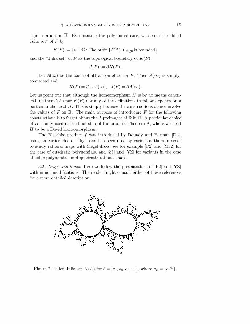
the Siegel disk for Pθ should correspond to the unit disk for Fθ, while theother bounded Fatou components of Pθ should correspond to other iteratedFθ-preimages of the unit disk, which we call drops. The basin of attractionof infinity for Pθ should correspond to a similar basin A(∞) for Fθ (which isthe immediate basin of attraction of infinity for fθ). By imitating the caseof polynomials, we define the “filled Julia set” K(Fθ) as C A(∞) and the“Julia set” J(Fθ) as the topological boundary of K(Fθ), both of which areindependent of the homeomorphism H (compare Figure 2).
By the results of Petersen and Lyubich mentioned above, J(Fθ) is locallyconnected and has measure zero for all irrational numbers θ. Thus, the local-connectivity statement in Theorem A will follow once we prove that for θ ∈ Ethere exists a homeomorphism ϕθ : C → C such that ϕθ Fθ ϕ−1
θ = Pθ.
4 C. L. PETERSEN AND S. ZAKERI
The measure zero statement in Theorem A will follow once we prove ϕθ isabsolutely continuous.
The basic idea described by Douady in [Do] is to choose the homeomorphicextension H in the definition of Fθ to be quasiconformal, which by Herman’stheorem is possible if and only if θ is of bounded type. Taking the Beltramidifferential of H on D, and spreading it by the iterated inverse branches ofFθ to all the drops, one obtains an Fθ-invariant Beltrami differential µ on Cwith bounded dilatation and with the support contained in the filled Juliaset K(Fθ). The measurable Riemann mapping theorem shows that µ can beintegrated by a quasiconformal homeomorphism which, when appropriatelynormalized, yields the desired conjugacy ϕθ.
To go beyond the bounded type class in the surgery construction, one hasto give up the idea of a quasiconformal surgery. The main idea, which webring to work here, is to use extensions H which are trans-quasiconformal, i.e.,have unbounded dilatation with controlled growth. What gives this approacha chance to succeed is the theorem of David on integrability of certain Beltramidifferentials with unbounded dilatation [Da]. David’s integrability conditionrequires that for all large K, the area of the set of points where the dilatationis greater than K be dominated by an exponentially decreasing function of K
(see subsection 2.5 for precise definitions). An orientation-preserving homeo-morphism between planar domains is a David homeomorphism if it belongs tothe Sobolev class W 1,1
loc and its Beltrami differential satisfies the above integra-bility condition. Such homeomorphisms are known to preserve the Lebesguemeasure class.
To carry out a trans-quasiconformal surgery, we have to address two fun-damental questions:
Question 1. Under what optimal arithmetical condition EDE on θ doesthe linearization hθ admit a David extension H : D → D?
Question 2. Under what optimal arithmetical condition EDI on θ doesthe model Fθ admit an invariant Beltrami differential satisfying David’s inte-grability condition in the plane?
It turns out that the two questions have the same answer, i.e., EDE = EDI.Clearly EDE ⊇ EDI, but the other inclusion is a nontrivial result, which weprove in this paper by means of the following construction.
Define a measure ν supported on D by summing up the push forward ofLebesgue measure on all the drops. In other words, for any measurable setE ⊂ D, set
ν(E) := area(E) +∑g
area(g(E)),
QUADRATIC POLYNOMIALS WITH A SIEGEL DISK 5
where the summation is over all the univalent branches g = F−kθ mapping D to
various drops. Evidently ν is absolutely continuous with respect to Lebesguemeasure on D. However, we prove a much sharper result:
Theorem B. The measure ν is dominated by a universal power of Lebesguemeasure. In other words, there exist a universal constant 0 < β < 1 and a con-stant C > 0 (depending on θ) such that
ν(E) ≤ C (area(E))β
for every measurable set E ⊂ D.
It follows immediately from this key estimate that the Fθ-invariant Bel-trami differential µ constructed above satisfies David’s integrability conditionif µ|D does, or equivalently, if there is a David extension H for hθ.
Theorem B can be used to prove that a conjugacy ϕθ between Fθ andPθ exists whenever hθ admits a David extension to the disk. The followingtheorem proves the existence of David extensions for circle homeomorphismswhich arise as linearizations of critical circle maps with rotation numbers in E .This theorem, as formulated here in the context of our trans-quasiconformalsurgery, is new. However, we should emphasize that all the main ingredientsof its constructive proof are already present in a manuscript of Yoccoz [Yo2].
Theorem C. Let f : S1 → S1 be a critical circle map whose rotationnumber θ = [a1, a2, a3, . . .] belongs to the arithmetical class E. Then the nor-malized linearizing map h : S1 → S1, which satisfies h f = Rθ h, admits aDavid extension H : D → D so that
area
z ∈ D :
∣∣∣∣∣∂H(z)∂H(z)
∣∣∣∣∣ > 1 − ε
≤ M e−
αε for all 0 < ε < ε0.
Here M > 0 is a universal constant, while in general the constant α > 0depends on lim supn→∞(log an)/
√n and the constant 0 < ε0 < 1 depends on f .
Let us point out that Theorem C proves E ⊂ EDE, where EDE is thearithmetical condition in Question 1. We have reasons to suspect that theabove inclusion might in fact be an equality, but so far we have not been ableto prove this.
When θ is of bounded type, the boundary of the Siegel disk ∆θ is aquasicircle, so it clearly has Hausdorff dimension less than 2. McMullen hasproved that in this case the entire Julia set Jθ has Hausdorff dimension lessthan 2 [Mc2], a result which improves the measure zero statement in Petersen’stheorem. The situation when θ belongs to E but is not of bounded typemight be quite different. In this case, the proof of Theorem A shows thatthe boundary of ∆θ is a David circle, i.e., the image of the round circle undera David homeomorphism. It can be shown that, unlike quasiconformal maps,
6 C. L. PETERSEN AND S. ZAKERI
David homeomorphisms do not preserve sets of Hausdorff dimension 0 or 2,and in fact there are David circles of Hausdorff dimension 2 [Z2]. So, a priori,the boundary of ∆θ might have Hausdorff dimension 2 as well. Motivated bythese remarks, we ask:
Question 3. What can be said about the Hausdorff dimension of Jθ whenθ belongs to E but is not of bounded type? Does there exist such a θ for whichJθ, or even ∂∆θ, has Hausdorff dimension 2?
The use of trans-quasiconformal surgery in holomorphic dynamics waspioneered by Haıssinsky who showed how to produce a parabolic point from apair of attracting and repelling points when the repelling point is not in theω-limit set of a recurrent critical point [Ha]. In contrast, our maps have arecurrent critical point whose orbit is dense in the boundary of the disk onwhich we perform surgery.
The idea of constructing rational maps by quasiconformal surgery onBlaschke products has been taken up by several authors; for instance Zakeri,who in [Z1] models the one-dimensional parameter space of cubic polynomialswith a Siegel disk of a given bounded type rotation number. Also this idea iscentral to the work of Yampolsky and Zakeri in [YZ], where they show thatany two quadratic Siegel polynomials Pθ1 and Pθ2 with bounded type rotationnumbers θ1 and θ2 are mateable provided that θ1 = 1 − θ2. We believe adap-tations of the ideas and techniques developed in the present paper will givegeneralizations of those results to rotation numbers in E .
Acknowledgements. The first author would like to thank the MathematicsDepartment of Cornell University for its hospitality and IMFUA at RoskildeUniversity for its financial support. The second author is grateful to IMS atStony Brook for supporting part of this research through NSF grant DMS9803242 during the spring semester of 1999. Further thanks are due to thereferee whose suggestions improved our presentation of puzzle pieces in Section4, and to P. Haıssinsky whose comment prompted us to add Lemma 5.5 toour early version of this paper.
2. Preliminaries
2.1. General notation. We will adopt the following notation throughoutthis paper:
• T is the quotient R/Z.
• S1 is the unit circle z ∈ C : |z| = 1; we often identify T and S1 via theexponential map x → e2πix without explicitly mentioning it.
QUADRATIC POLYNOMIALS WITH A SIEGEL DISK 7
• |I| is the Euclidean length of a rectifiable arc I ⊂ C.
• For x, y ∈ T or S1 which are not antipodal, [x, y] = [y, x] (resp. ]x, y[ =]y, x[) denotes the shorter closed (resp. open) interval with endpoints x, y.
• diam(·), dist(·, ·) and area(·) denote the Euclidean diameter, Euclideandistance and Lebesgue measure in C.
• For a hyperbolic Riemann surface X, X(·), diamX(·) and distX(·) denotethe hyperbolic arclength, diameter and distance in X.
• In a given statement, by a universal constant we mean one which is inde-pendent of all the parameters/variables involved. Two positive numbersa, b are said to be comparable up to a constant C > 1 if b/C ≤ a ≤ b C.For two positive sequences an and bn, we write an bn if there ex-ists a universal constant C > 1 such that an ≤ C bn for all large n. Wedefine an bn in a similar way. We write an bn if bn an bn, i.e., ifthere exists a universal constant C > 1 such that bn/C ≤ an ≤ C bn forall large n. Any such relation will be called an asymptotically universalbound. Note that for any such bound, the corresponding inequalities holdfor every n if C is replaced by a larger constant (which may well dependon our sequences and no longer be universal).
Another way of expressing an asymptotically universal bound, which wewill often use, is as follows: When an bn, we say that an/bn is boundedfrom above by a constant which is asymptotically universal. Similarly,when an bn, we say that an and bn are comparable up to a constantwhich is asymptotically universal.
Finally, let an = an(x) and bn = bn(x) depend on a parameter x
belonging to a set X. Then we say that an bn uniformly in x ∈ X ifthere exists a universal constant C > 1 and an integer N ≥ 1 such thatbn(x)/C ≤ an(x) ≤ Cbn(x) for all n ≥ N and all x ∈ X.
2.2. Some arithmetic. Here we collect some basic facts about continuedfractions; see [Kh] or [La] for more details. Let 0 < θ < 1 be an irrationalnumber and consider the continued fraction expansion
θ =1
a1 + 1a2 +
1a3 + · · ·
= [a1, a2, a3, . . .],
with an = an(θ) ∈ N. The n-th convergent of θ is the irreducible fractionpn/qn := [a1, a2, . . . , an]. We set p0 := 0, q0 := 1. It is easy to verify therecursive relations
(2.1) pn = an pn−1 + pn−2 and qn = an qn−1 + qn−2
8 C. L. PETERSEN AND S. ZAKERI
for n ≥ 2. The denominators qn grow exponentially fast; in fact it followseasily from (2.1) that
qn ≥ (√
2)n for n ≥ 2.
Elementary arithmetic shows that
(2.2)1
qn(qn + qn+1)<
∣∣∣∣θ − pn
qn
∣∣∣∣ <1
qnqn+1,
which implies pn/qn → θ exponentially fast.Various arithmetical conditions on irrational numbers come up in the
study of indifferent fixed points of holomorphic maps. Of particular interestare:
• The class Dd of Diophantine numbers of exponent d ≥ 2. An irrational θ
belongs to Dd if there exists some C > 0 such that |θ − p/q| ≥ Cq−d forall rationals p/q. It follows immediately from (2.2) that for any d ≥ 2
(2.3) θ ∈ Dd ⇔ supn
qn+1
qnd−1
< +∞ ⇔ supn
an+1
qnd−2
< +∞.
• The class D :=⋃
d≥2 Dd of Diophantine numbers. From (2.3) it followsthat
θ ∈ D ⇔ supn
log qn+1
log qn< +∞.
• The class D2 of Diophantine numbers of exponent 2. Again by (2.3)
θ ∈ D2 ⇔ supn
an < +∞.
For this reason, any such θ is called a number of bounded type.
• The class B of numbers of Brjuno type. By definition,
θ ∈ B ⇔∞∑
n=1
log qn+1
qn< +∞.
We have the proper inclusions
D2 Dd D B
for any d > 2. Diophantine numbers of any exponent d > 2 have full measurein [0, 1] while numbers of bounded type form a set of measure zero.
The following theorem characterizes the asymptotic growth of the se-quence an for random irrational numbers:
QUADRATIC POLYNOMIALS WITH A SIEGEL DISK 9
Theorem 2.1. Let ψ : N → R be a given positive function.
(i) If∑∞
n=11
ψ(n) < +∞, then for almost every irrational 0 < θ < 1 there areonly finitely many n for which an(θ) ≥ ψ(n).
(ii) If∑∞
n=11
ψ(n) = +∞, then for almost every irrational 0 < θ < 1 there areinfinitely many n for which an(θ) ≥ ψ(n).
This theorem is often attributed to E. Borel and F. Bernstein, at least inthe case ψ is increasing. For a proof of the general case, see Khinchin’s book[Kh].
Corollary 2.2. Let E be the set of all irrational numbers 0 < θ < 1 forwhich the sequence an = an(θ) satisfies
(2.4) log an = O(√
n) as n → ∞.
Then E has full measure in [0, 1].
The class E will be the center of focus in the present paper. It is easilyseen to be a proper subclass of Dd for any d > 2.
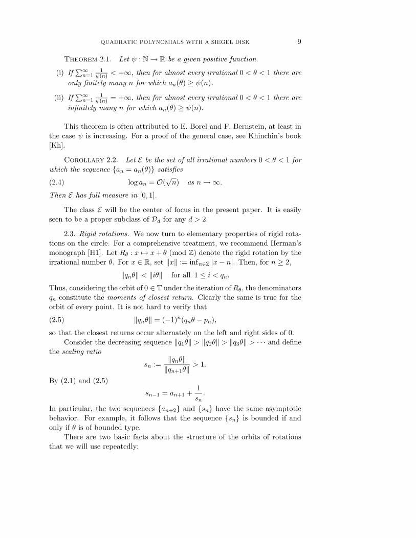
2.3. Rigid rotations. We now turn to elementary properties of rigid rota-tions on the circle. For a comprehensive treatment, we recommend Herman’smonograph [H1]. Let Rθ : x → x + θ (mod Z) denote the rigid rotation by theirrational number θ. For x ∈ R, set ‖x‖ := infn∈Z |x − n|. Then, for n ≥ 2,
‖qnθ‖ < ‖iθ‖ for all 1 ≤ i < qn.
Thus, considering the orbit of 0 ∈ T under the iteration of Rθ, the denominatorsqn constitute the moments of closest return. Clearly the same is true for theorbit of every point. It is not hard to verify that
(2.5) ‖qnθ‖ = (−1)n(qnθ − pn),
so that the closest returns occur alternately on the left and right sides of 0.Consider the decreasing sequence ‖q1θ‖ > ‖q2θ‖ > ‖q3θ‖ > · · · and define
the scaling ratio
sn :=‖qnθ‖‖qn+1θ‖
> 1.
By (2.1) and (2.5)
sn−1 = an+1 +1sn
.
In particular, the two sequences an+2 and sn have the same asymptoticbehavior. For example, it follows that the sequence sn is bounded if andonly if θ is of bounded type.
There are two basic facts about the structure of the orbits of rotationsthat we will use repeatedly:
10 C. L. PETERSEN AND S. ZAKERI
• For i ∈ Z, let xi denote the iterate R−iθ (0) (Caution: We have labelled
the orbit of 0 backwards to simplify the subsequent notations; this cor-responds to the standard notation for the inverse map R−1
θ ). Given twoconsecutive closest return moments qn and qn+1, the points in the orbitof 0 occur in the order shown in Figure 1 (the picture shows the case n isodd; for the case n is even simply rotate the picture 180 about 0). Notethat |[0, xqn ]| = |[0, x−qn ]| = ‖qnθ‖. Evidently, the orbit of any otherpoint of T enjoys the same order.
xqn+1xqn+1 qn qn-1
xqn + xqn-1
...0nqx x qn+1
Figure 1. Selected points in the orbit of 0 under the rigid rotation.
• Let In := [0, xqn ] be the n-th closest return interval for 0. Then thecollection of intervals
(2.6) Πn(Rθ) := R−iθ (In)0≤i≤qn+1−1 ∪ R−i
θ (In+1)0≤i≤qn−1
defines a partition of the circle modulo the common endpoints. We callΠn(Rθ) the dynamical partition of level n for Rθ.
Theorem 2.3 (Poincare). Let f : T → T be any circle homeomorphismwithout periodic points. Then there exists a unique irrational number θ and acontinuous degree 1 monotone map h : T → T such that h f = Rθ h.
The number θ is called the rotation number of f and is denoted by ρ(f).The map h is called a Poincare semiconjugacy. It easily follows from thistheorem that the combinatorial structure of the orbits of any circle homeo-morphism with irrational rotation number θ is the same as the combinatorialstructure of the orbit of 0 for Rθ.
2.4. Critical circle maps. For our purposes, a critical circle map will bea real-analytic homeomorphism of T with a critical point at 0. It was provedby Yoccoz [Yo1] that for a critical circle map with irrational rotation number,every Poincare semiconjugacy is in fact a conjugacy:
Theorem 2.4 (Yoccoz). Let f : T → T be a critical circle map withirrational rotation number ρ(f) = θ. Then there exists a homeomorphismh : T → T such that h f = Rθ h. This h is uniquely determined oncenormalized by h(0) = 0.
We will reserve the notation xi for the backward iterate f−i(0) of thecritical point 0 and In := [0, xqn ] for the n-th closest return interval under f−1.
QUADRATIC POLYNOMIALS WITH A SIEGEL DISK 11
The dynamical partition Πn(f) of level n for f will be defined as h−1(Πn(Rθ)),or equivalently, by (2.6) with Rθ replaced by f .
Herman took the next step in studying critical circle maps by showingthat the linearizing map h is quasisymmetric if and only if ρ(f) is irrational ofbounded type. The proof of this theorem makes essential use of the existenceof real a priori bounds developed by Swiatek and Herman. Here is a version oftheir result needed in this paper (see [Sw], [H2], [dFdM], or [P4]).
Theorem 2.5 (Swiatek-Herman). Let f : T → T be a critical circle mapwith ρ(f) irrational. Then
(i) There exists an asymptotically universal bound
|[y, fqn(y)]| |[y, f−qn(y)]|
which holds uniformly in y ∈ T.
(ii) The lengths of any two adjacent intervals in the dynamical partitionΠn(f) are comparable up to a bound which is asymptotically universal.In other words,
max |I||J | : I, J ∈ Πn(f) are adjacent
1.
An important corollary of (ii), which exhibits a sharp contrast with thecase of rigid rotations, is that the scaling ratio is bounded from above andbelow by an asymptotically universal constant regardless of the map f :
sn(f) :=|In||In+1| 1.
Remark 2.6. The above (i) and (ii) are presumably the most generalstatements one can expect when working with the class of all critical circlemaps. However, stronger versions of these bounds can be obtained by restrict-ing to a special class of such maps. For example, fix a critical circle map f0
and consider the one-dimensional family
F = Rt f0 : 0 ≤ t ≤ 1 and ρ(Rt f0) is irrational.
Then, within this family the above bounds hold for all n (rather than all largen), with the constant depending only on f0 and not on t. In other words, thereexists a constant C = C(f0) > 1 such that
1C
≤ |[y, fqn(y)]||[y, f−qn(y)]| ≤ C for all n ≥ 1, y ∈ T, and f ∈ F ,
1C
≤ max |I||J | : I, J ∈ Πn(f) are adjacent
≤ C for all n ≥ 1 and f ∈ F .
12 C. L. PETERSEN AND S. ZAKERI
We will need the following result on the size of the intervals in the dy-namical partitions for a critical circle map; it is a direct consequence of reala priori bounds (see for example [dFdM, Th. 3.1]):
Lemma 2.7. Let f : T → T be a critical circle map, with ρ(f) irrational,and let Πn(f) denote the dynamical partition of level n for f . Then there existuniversal constants 0 < σ1 < σ2 < 1 such that
σn1 |In| ≤ max
I∈Πn(f)|I| σn
2 .
2.5. David homeomorphisms. An orientation-preserving homeomorphismϕ : Ω → Ω′ between planar domains belongs to the Sobolev class W 1,1
loc (Ω) ifthe distributional partial derivatives ∂ϕ and ∂ϕ exist and are locally integrablein Ω (equivalently, if ϕ is absolutely continuous on lines in Ω; see for example[A]). In this case, ϕ is differentiable almost everywhere and the JacobianJac(ϕ) = |∂ϕ|2 − |∂ϕ|2 ≥ 0 is locally integrable.
A Beltrami differential in Ω is a measurable (−1, 1)-form µ = µ(z) dz/dz
such that |µ| < 1 almost everywhere in Ω. We say that µ is integrable if there isa homeomorphism ϕ : Ω → Ω′ in W 1,1
loc (Ω) which solves the Beltrami equation∂ϕ = µ ∂ϕ. The classical quasiconformal mappings arise as the solutions ofthe Beltrami equation in the case ‖µ‖∞ < 1. However, there are numerousimportant problems in which one has to study this equation when ‖µ‖∞ = 1.Simple examples show that such a µ is not generally integrable, so one has toseek conditions on the growth of |µ| which guarantee integrability. One suchcondition was given by Guy David in [Da], who studied Beltrami differentialssatisfying an exponential growth condition. Let us call µ a David-Beltramidifferential if there exist constants M > 0, α > 0, and 0 < ε0 < 1 such that
(2.7) areaz ∈ Ω : |µ|(z) > 1 − ε ≤ M e−αε for all 0 < ε < ε0.
This notion can be extended to arbitrary domains on the sphere C; it sufficesto replace the Euclidean area with the spherical area in the growth condition(2.7).
David proved that the analogue of the measurable Riemann mapping the-orem [AB] holds for the class of David-Beltrami differentials [Da]:
Theorem 2.8 (David). Let Ω be a domain in C and µ be a David -Beltrami differential in Ω. Then µ is integrable. More precisely, there exists anorientation-preserving homeomorphism ϕ : Ω → Ω′ in W 1,1
loc (Ω) which satisfies∂ϕ = µ ∂ϕ almost everywhere. Moreover, ϕ is unique up to postcompositionwith a conformal map. In other words, if Φ : Ω → Ω′′ is another homeomorphicsolution of the same Beltrami equation in W 1,1
loc (Ω), then Φ ϕ−1 : Ω′ → Ω′′ isa conformal map.
QUADRATIC POLYNOMIALS WITH A SIEGEL DISK 13
Solutions of the Beltrami equation given by this theorem are called Davidhomeomorphisms. They differ from classical quasiconformal maps in manyrespects. A significant example is the fact that the inverse of a David home-omorphism is not necessarily David. However, they enjoy some convenientproperties of quasiconformal maps such as compactness; see [T] for a study ofsome of these similarities. The following result is particularly important [Da]:
Theorem 2.9. Let ϕ : Ω → Ω′ be a David homeomorphism. Then ϕ
and ϕ−1 are both absolutely continuous; in other words, for a measurable setE ⊂ Ω,
area(E) = 0 ⇐⇒ area(ϕ(E)) = 0.
It easily follows that if ϕ : Ω → Ω′ is a David homeomorphism, then∂ϕ = 0 almost everywhere in Ω. Thus, the complex dilatation of ϕ, defined bythe measurable (−1, 1)-form
µϕ :=∂ϕ
∂ϕ
dz
dz
is a well-defined David-Beltrami differential in the sense of (2.7). Equivalently,the real dilatation of ϕ, given by
Kϕ :=1 + |µϕ|1 − |µϕ|
,
satisfies a condition of the form
(2.8) areaz ∈ Ω : Kϕ(z) > K ≤ M e−αK for all K > K0
for some constants M > 0, α > 0, and K0 > 1.
2.6. Extensions of linearizing homeomorphisms. Let f be a critical circlemap with ρ(f) irrational and consider the linearizing map h given by Yoc-coz’s Theorem 2.4. The problem of extending h to a self-homeomorphism ofthe disk with nice analytic properties arises in various circumstances in holo-morphic dynamics, particularly in the construction of Siegel disks by meansof surgery. When ρ(f) is of bounded type, it follows from Theorem 2.5 thath is quasisymmetric. Hence, by the theorem of Beurling-Ahlfors [BA], it canbe extended to a quasiconformal map D → D whose dilatation only dependson the quasisymmetric norm of h (which in turn only depends on supn an(θ),where θ = ρ(f)). This allows a quasiconformal surgery (compare [Do], [P2],[Z1], or [YZ]).
On the other hand, when ρ(f) is not of bounded type, again by Theo-rem 2.5, h fails to be quasisymmetric and hence it admits no quasiconformalextension. Thus, one is forced to give up the idea of quasiconformal surgery.
Still, one can ask if in this case h admits a David extension to D. Oneway to address this problem is to develop a Beurling-Ahlfors theory for David
14 C. L. PETERSEN AND S. ZAKERI
homeomorphisms of the disk. For example, it is possible to show that a circlehomeomorphism whose local distortion has controlled growth admits a Davidextension. But, to the best of our knowledge, the problem of characterizingboundary values of David homeomorphisms has not yet been solved completely:
Problem. Find necessary and sufficient conditions for a circle homeomor-phism to admit a David extension to the unit disk.
Another approach, less general but very effective in our dynamical frame-work, is to attempt to construct David extensions directly for the circle home-omorphisms which arise as linearizing maps of critical circle maps. This ap-proach turns out to be successful because of the existence of real a prioribounds (Theorem 2.5). In fact, using Yoccoz’s work in [Yo2], one can provethe following:
Theorem C. Let f : S1 → S1 be a critical circle map whose rotationnumber θ = [a1, a2, a3, . . .] belongs to the arithmetical class E defined in (2.4).Then the linearizing map h : S1 → S1, which satisfies h f = Rθ h andh(1) = 1, admits a David extension H : D → D. Moreover, the constantM in condition (2.7) is universal, while in general α depends onlim supn→∞(log an)/
√n and ε0 depends on f .
The proof of this result is rather lengthy and will be presented in theappendix.
3. A Blaschke model
3.1. Definitions. Given an irrational number 0 < θ < 1, consider thedegree 3 Blaschke product
(3.1) f = fθ : z → e2πit(θ) z2(
z − 31 − 3z
),
which has superattracting fixed points at 0 and ∞ and a double critical pointat z = 1. Here 0 < t(θ) < 1 is the unique parameter for which the critical circlemap f |S1 : S1 → S1 has rotation number θ. By Theorem 2.4, there exists aunique homeomorphism h : S1 → S1 with h(1) = 1 such that h f |S1 = Rθ h.Let H : D → D be any homeomorphic extension of h and define
(3.2) F (z) = Fθ,H(z) :=
f(z) if |z| ≥ 1
(H−1 Rθ H)(z) if |z| < 1.
It is easy to see that F is a degree 2 topological branched covering of thesphere which is holomorphic outside of D and is topologically conjugate to a
QUADRATIC POLYNOMIALS WITH A SIEGEL DISK 15
rigid rotation on D. By imitating the polynomial case, we define the “filledJulia set” of F by
K(F ) := z ∈ C : The orbit F n(z)n≥0 is bounded
and the “Julia set” of F as the topological boundary of K(F ):
J(F ) := ∂K(F ).
Let A(∞) be the basin of attraction of ∞ for F . Then A(∞) is simply-connected and
K(F ) = C A(∞), J(F ) = ∂A(∞).
Let us point out that although the homeomorphism H is by no means canon-ical, neither J(F ) nor K(F ) nor any of the definitions to follow depends on aparticular choice of H. This is simply because the constructions do not involvethe values of F on D. The main purpose of introducing F for the followingconstructions is to forget about the f -preimages of D in D. A particular choiceof H is only used in the final step of the proof of Theorem A, where we needH to be a David homeomorphism.
The Blaschke product f was introduced by Douady and Herman [Do],using an earlier idea of Ghys, and has been used by various authors in orderto study rational maps with Siegel disks; see for example [P2] and [Mc2] forthe case of quadratic polynomials, and [Z1] and [YZ] for variants in the caseof cubic polynomials and quadratic rational maps.
3.2. Drops and limbs. Here we follow the presentations of [P2] and [YZ]with minor modifications. The reader might consult either of these referencesfor a more detailed description.
Figure 2. Filled Julia set K(F ) for θ = [a1, a2, a3, . . .], where an = e√
n.

16 C. L. PETERSEN AND S. ZAKERI
By definition, the unique component of F−1(D) D is called the 0-dropof F and is denoted by U0. (In Figure 2, U0 is the prominently visible Jordandomain attached to the unit disk at z = 1.) For n ≥ 1, any component U ofF−n(U0) is a Jordan domain called an n-drop, with n being the depth of U .The map F n = fn : U → U0 is a conformal isomorphism which extendsisomorphically to a neighborhood of U , because U0 does not intersect theforward orbit of the critical values. The unique point F−n(1) ∩ ∂U is calledthe root of U and is denoted by x(U). The boundary ∂U is a real-analyticJordan curve except at the root where it has an angle of π/3. We simply referto U as a drop when the depth is not important. For convenience, we defineD to be a (−1)-drop, i.e., a drop of depth −1. Note that these drops do notdepend on the extension H used to define the map F in (3.2).
Let U and V be distinct drops of depths m and n, respectively, withm ≤ n. Then either U ∩ V = ∅ or else U ∩ V = x(V ) and m < n. In the lattercase, we call U the parent of V , and V a child of U . Every n-drop with n ≥ 0has a unique parent which is an m-drop with −1 ≤ m < n. In particular, theroot of this n-drop belongs to the boundary of its parent.
By definition, D is said to be of generation 0. Any child of D is of gen-eration 1. In general, a drop is of generation k if and only if its parent is ofgeneration k − 1. Given a point w ∈ ⋃
n≥0 F−n(1), there exists a unique dropU with x(U) = w. In particular, two distinct children of a parent have distinctroots.
We give a symbolic description of drops by assigning addresses to them.Set U∅ := D, where ∅ is the empty index. For n ≥ 0, let xn := F−n(1) ∩ S1
and let Un be the n-drop of generation 1 with root xn. Let ι = ι1, ι2, . . . , ιk beany multi-index of length k ≥ 1, where each ιj is a nonnegative integer. Werecursively define the (ι1+ι2+· · ·+ιk)-drop Uι1,ι2,...,ιk of generation k with rootx(Uι1,ι2,...,ιk) = xι1,ι2,...,ιk as follows. We have already defined these for k = 1.Suppose that we have defined xι1,ι2,...,ιk−1
for all multi-indices ι1, ι2, . . . , ιk−1 oflength k − 1. Then, we define
xι1,ι2,...,,ιk := F−(1+ι1)(xι2,...,ιk) ∩ ∂Uι1,ι2,...,ιk−1.
The drop Uι1,ι2,...,ιk will be determined by the condition of having xι1,ι2,...,ιk asits root. By the way these drops have been given addresses, we have
F (Uι1,ι2,...,ιk) =
Uι2,...,ιk if ι1 = 0
Uι1−1,ι2,...,ιk if ι1 > 0.
Let us fix a drop Uι1,...,ιk . By definition, the limb Lι1,...,ιk is the closureof the union of this drop and all its descendants, i.e., children, grandchildren,etc.:
Lι1,...,ιk :=⋃
Uι1,...,ιk,··· .
QUADRATIC POLYNOMIALS WITH A SIEGEL DISK 17
The integers k and ι1 + · · · + ιk are called generation and depth of the limbLι1,...,ιk , respectively. Any two limbs are either disjoint or nested. Moreover,for any limb Lι1,...,ιk , we have
F (Lι1,...,ιk) =
Lι2,...,ιk if ι1 = 0
Lι1−1,ι2,...,ιk if ι1 > 0.
In particular, every limb eventually maps to L0 and then to the entire filledJulia set L∅ = K(F ).
3.3. Main results on J(F ). The Julia set J(F ) = J(Fθ,H) serves as amodel for the Julia set Jθ of the quadratic polynomial Pθ : z → e2πiθz + z2
when Jθ is locally connected. In fact, it follows from the next theorem that F
and Pθ are topologically conjugate if and only if Jθ is locally connected:
Theorem 3.1 (Petersen). For every irrational 0 < θ < 1 the Julia setJ(F ) is locally connected.
See [P2] for the original proof as well as [Ya] and [P3] for a simplifiedversion of it. The central theme of the proof is the fact that the Euclideandiameter of a limb Lι1,...,ιk tends to 0 as its depth ι1 + · · · + ιk tends to ∞.
Another issue is the Lebesgue measure of these Julia sets:
Theorem 3.2 (Petersen, Lyubich). For every irrational 0 < θ < 1 theJulia set J(F ) has Lebesgue measure zero.
This theorem was first proved in [P2] for θ of bounded type. The proof ofthe general case, suggested by Lyubich, can be found in [Ya].
4. Puzzle pieces and a priori area estimates
4.1. The dyadic puzzle. This subsection outlines the construction of puzzlepieces and recalls their basic properties. Much of the material here can be foundin greater detail in [P2] and [P3].
Let R0 denote the closure of the fixed external ray landing at the re-pelling fixed point β ∈ CD of F . Similarly, let R1/2 := F−1(R0)R0 denotethe closure of the external ray landing at the preimage of β (for landing of(pre)periodic rays, see for example [DH1], [P1], or [TY]). Let E be the equipo-tential z : G(z) = 1, where G : A(∞) → R is the Green’s function on thebasin of infinity. The set
C (R0 ∪R1/2 ∪ E ∪ D ∪ U0 ∪ U00 ∪ U000 ∪ · · · ∪ U1 ∪ U10 ∪ U100 ∪ · · ·)has two bounded connected components which are Jordan domains. Let P1,0
be the closure of that component which intersects the external rays with angles
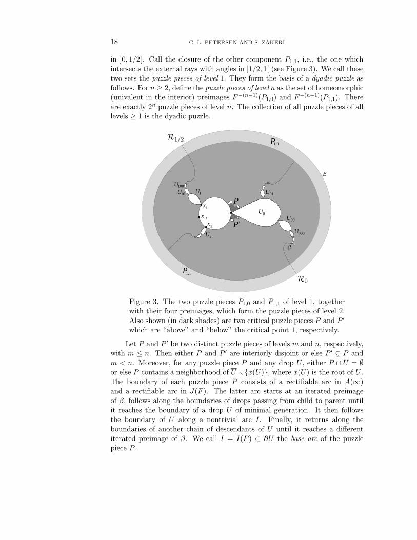
18 C. L. PETERSEN AND S. ZAKERI
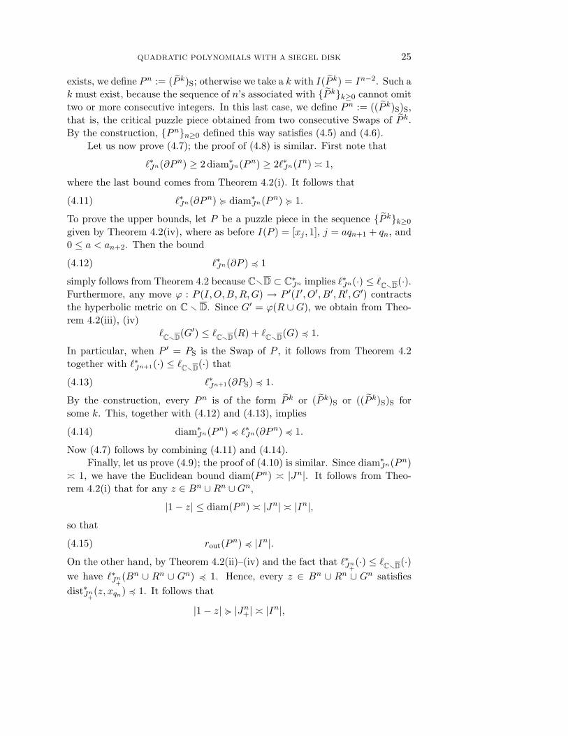
in ]0, 1/2[. Call the closure of the other component P1,1, i.e., the one whichintersects the external rays with angles in ]1/2, 1[ (see Figure 3). We call thesetwo sets the puzzle pieces of level 1. They form the basis of a dyadic puzzle asfollows. For n ≥ 2, define the puzzle pieces of level n as the set of homeomorphic(univalent in the interior) preimages F−(n−1)(P1,0) and F−(n−1)(P1,1). Thereare exactly 2n puzzle pieces of level n. The collection of all puzzle pieces of alllevels ≥ 1 is the dyadic puzzle.
P
1
100
10
P
E
P
U
x
2xx
1,0
P01U
U
U
1,1
2
UU
0
00
U000
β
U
1
1
1
R1/2
R0
Figure 3. The two puzzle pieces P1,0 and P1,1 of level 1, togetherwith their four preimages, which form the puzzle pieces of level 2.Also shown (in dark shades) are two critical puzzle pieces P and P ′
which are “above” and “below” the critical point 1, respectively.
Let P and P ′ be two distinct puzzle pieces of levels m and n, respectively,with m ≤ n. Then either P and P ′ are interiorly disjoint or else P ′ P andm < n. Moreover, for any puzzle piece P and any drop U , either P ∩ U = ∅or else P contains a neighborhood of U x(U), where x(U) is the root of U .The boundary of each puzzle piece P consists of a rectifiable arc in A(∞)and a rectifiable arc in J(F ). The latter arc starts at an iterated preimageof β, follows along the boundaries of drops passing from child to parent untilit reaches the boundary of a drop U of minimal generation. It then followsthe boundary of U along a nontrivial arc I. Finally, it returns along theboundaries of another chain of descendants of U until it reaches a differentiterated preimage of β. We call I = I(P ) ⊂ ∂U the base arc of the puzzlepiece P .
QUADRATIC POLYNOMIALS WITH A SIEGEL DISK 19
A puzzle piece P is called critical if it contains the critical point x0 = 1.The critical puzzle piece P1,0 is said to be “above” (the critical point 1), becauseits intersection with a small disk around 1 is contained in the closed upper half-plane; similarly P1,1 is said to be “below”. More generally, a critical puzzlepiece P is “above” if P ⊂ P1,0 and “below” if P ⊂ P1,1 (compare Figure 3).
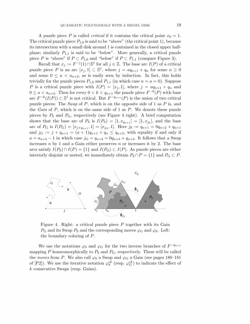
Recall that xj := F−j(1)∩S1 for all j ∈ Z. The base arc I(P ) of a criticalpuzzle piece P is an arc [xj , 1] ⊂ S1, where j = aqn+1 + qn for some n ≥ 0and some 0 ≤ a < an+2, as is easily seen by induction. In fact, this holdstrivially for the puzzle pieces P1,0 and P1,1 (in which case n = a = 0). SupposeP is a critical puzzle piece with I(P ) = [xj , 1], where j = aqn+1 + qn and0 ≤ a < an+2. Then for every 0 < k < qn+1 the puzzle piece F−k(P ) with basearc F−k(I(P )) ⊂ S1 is not critical. But F−qn+1(P ) is the union of two criticalpuzzle pieces: The Swap of P , which is on the opposite side of 1 as P is, andthe Gain of P , which is on the same side of 1 as P . We denote these puzzlepieces by PS and PG, respectively (see Figure 4 right). A brief computationshows that the base arc of PS is I(PS) = [1, xqn+1 ] = [1, xjS ], and the basearc of PG is I(PG) = [xj+qn+1 , 1] = [xjG , 1]. Here jS := qn+1 = 0qn+2 + qn+1
and jG := j + qn+1 = (a + 1)qn+1 + qn ≤ qn+2, with equality if and only ifa = an+2 − 1 in which case jG = qn+2 = 0qn+3 + qn+2. It follows that a Swapincreases n by 1 and a Gain either preserves n or increases it by 2. The basearcs satisfy I(PS)∩ I(P ) = 1 and I(PG) ⊂ I(P ). As puzzle pieces are eitherinteriorly disjoint or nested, we immediately obtain PS∩P = 1 and PG ⊂ P .
I
RO
B
G
P
x
P
j
PG
S
x
xi0,U
0,i
1 S
j
xjGj
U
G
S
U0
ϕ
ϕ
Figure 4. Right: a critical puzzle piece P together with its GainPG and its Swap PS and the corresponding moves ϕG and ϕS. Left:the boundary coloring of P .
We use the notations ϕS and ϕG for the two inverse branches of F−qn+1
mapping P homeomorphically to PS and PG, respectively. These will be calledthe moves from P . We also call ϕS a Swap and ϕG a Gain (see pages 180–181of [P2]). We use the iterative notation ϕk
S (resp. ϕkG ) to indicate the effect of
k consecutive Swaps (resp. Gains).
20 C. L. PETERSEN AND S. ZAKERI
In order to make precise references to the constructions in [P2], we needto reproduce the definition of “boundary coloring” here. This is a partitionof the boundary of each critical puzzle piece P into five closed and interiorlydisjoint arcs I, O, B, R and G defined as follows (compare Figure 4 left):
• The base arc I = I(P ) = P ∩ S1 = [xj , 1], with j = aqn+1 + qn and0 ≤ a < an+2, has already been defined.
• The Orange arc O = O(P ) := P∩∂U0 = [1, x0,i], where i = bqn+qn−1−1,1 ≤ b ≤ an+1, and n is given by j as above. Here and in what follows,the notation [1, x0,i] indicates the shorter subarc of ∂U0 with endpoints1 and x0,i. (For a comparison, note that in [P2] the point x0,i is denotedby yi+1.)
• The Blue arc B = B(P ) := P ∩ ∂Uj , with j as above.
• The Red arc R = R(P ) := P ∩ ∂U0,i, with i as above.
• Finally, the Green arc G = G(P ) is the closure of the complementary arc∂P (I ∪ O ∪ B ∪ R).
In what follows, P (I, O, B, R, G) will denote the critical puzzle piece withboundary arcs I, O, B, R, G. Note that the arcs R and G of any critical puzzlepiece are compact subsets of C D.
The relation between boundary colorings and moves is as follows. Suppose
ϕ : P ′(I ′, O′, B′, R′, G′) → P (I, O, B, R, G)
is a move from the critical puzzle piece P ′ to the critical puzzle piece P . Then
ϕ(I ′) = I ∪ O ϕ(R′ ∪ G′) = G.
Moreover, if ϕ = ϕS is a Swap, then
ϕS(O′) = B ϕS(B′) = R,
while if ϕ = ϕG is a Gain, then
ϕG(O′) = R ϕG(B′) = B.
One can use the above relations to verify that neither I, O nor evenI, O, B, R can determine a puzzle piece P uniquely. In fact, if P is a criti-cal puzzle piece with I(P ) = [xqn , 1], it follows from the definitions of Swapand Gain that the two puzzle pieces P1 = ϕ2
S (P ) and P2 = ϕan+2
G (P ) aredistinct but have identical base arcs I(P1) = I(P2) = [xqn+2 , 1]. On the otherhand, if P1 and P2 are two distinct critical puzzle pieces with the same basearc I(P1) = I(P2), the above relations show that the two puzzle pieces ϕ3
S (P1)and ϕ3
S (P2) are distinct but have identical I, O, B, R boundary arcs.
QUADRATIC POLYNOMIALS WITH A SIEGEL DISK 21
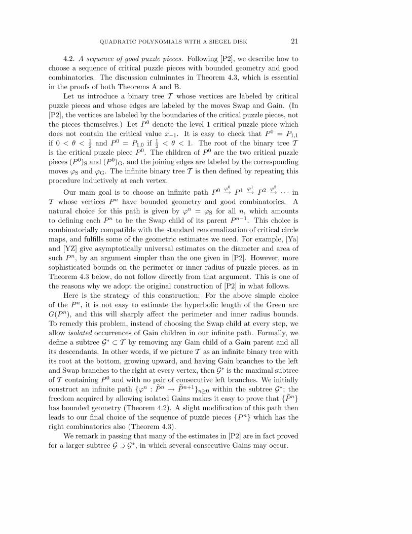
4.2. A sequence of good puzzle pieces. Following [P2], we describe how tochoose a sequence of critical puzzle pieces with bounded geometry and goodcombinatorics. The discussion culminates in Theorem 4.3, which is essentialin the proofs of both Theorems A and B.
Let us introduce a binary tree T whose vertices are labeled by criticalpuzzle pieces and whose edges are labeled by the moves Swap and Gain. (In[P2], the vertices are labeled by the boundaries of the critical puzzle pieces, notthe pieces themselves.) Let P 0 denote the level 1 critical puzzle piece whichdoes not contain the critical value x−1. It is easy to check that P 0 = P1,1
if 0 < θ < 12 and P 0 = P1,0 if 1
2 < θ < 1. The root of the binary tree Tis the critical puzzle piece P 0. The children of P 0 are the two critical puzzlepieces (P 0)S and (P 0)G, and the joining edges are labeled by the correspondingmoves ϕS and ϕG. The infinite binary tree T is then defined by repeating thisprocedure inductively at each vertex.
Our main goal is to choose an infinite path P 0 ϕ0
→ P 1 ϕ1
→ P 2 ϕ2
→ · · · inT whose vertices Pn have bounded geometry and good combinatorics. Anatural choice for this path is given by ϕn = ϕS for all n, which amountsto defining each Pn to be the Swap child of its parent Pn−1. This choice iscombinatorially compatible with the standard renormalization of critical circlemaps, and fulfills some of the geometric estimates we need. For example, [Ya]and [YZ] give asymptotically universal estimates on the diameter and area ofsuch Pn, by an argument simpler than the one given in [P2]. However, moresophisticated bounds on the perimeter or inner radius of puzzle pieces, as inTheorem 4.3 below, do not follow directly from that argument. This is one ofthe reasons why we adopt the original construction of [P2] in what follows.
Here is the strategy of this construction: For the above simple choiceof the Pn, it is not easy to estimate the hyperbolic length of the Green arcG(Pn), and this will sharply affect the perimeter and inner radius bounds.To remedy this problem, instead of choosing the Swap child at every step, weallow isolated occurrences of Gain children in our infinite path. Formally, wedefine a subtree G∗ ⊂ T by removing any Gain child of a Gain parent and allits descendants. In other words, if we picture T as an infinite binary tree withits root at the bottom, growing upward, and having Gain branches to the leftand Swap branches to the right at every vertex, then G∗ is the maximal subtreeof T containing P 0 and with no pair of consecutive left branches. We initiallyconstruct an infinite path ϕn : Pn → Pn+1n≥0 within the subtree G∗; thefreedom acquired by allowing isolated Gains makes it easy to prove that Pnhas bounded geometry (Theorem 4.2). A slight modification of this path thenleads to our final choice of the sequence of puzzle pieces Pn which has theright combinatorics also (Theorem 4.3).
We remark in passing that many of the estimates in [P2] are in fact provedfor a larger subtree G ⊃ G∗, in which several consecutive Gains may occur.
22 C. L. PETERSEN AND S. ZAKERI
Definition 4.1. For an open interval J S1, define the hyperbolic domain
(4.1) C∗J := (C∗ S1) ∪ J.
The simplified notation ∗J(·) = C∗J(·), diam∗
J(·) = diamC∗J(·) and dist∗J(·) =
distC∗J(·) will be used for the hyperbolic arclength, diameter and distance in C∗
J .
For n ≥ 0, let
Jn := ]x−qn+1+qn , x−qn [ and Jn+ := ]x−qn+1+qn , 1[.
Note thatIn 1 = [xqn , 1[ Jn
+ Jn.
The main technical tool in [P2] is the following collection of estimates on thelength of the boundary arcs of critical puzzle pieces.
Theorem 4.2. Let P (I, O, B, R, G) be a critical puzzle piece with thebase arc I = [xj , 1], where j = aqn+1 + qn and 0 ≤ a < an+2. Let J = Jn andJ+ = Jn
+. Then the following asymptotically universal bounds hold :
(i) |O| |I| and ∗J(O) ∗J(I) 1.
Moreover, if P is a vertex of G∗, then
(ii) ∗J(B) ∗J+(B) 1,
(iii) CD(R) 1.
Finally, there exists an infinite path ϕk : P k → P k+1k≥0 in G∗, starting atthe root P 0 = P 0, such that
(iv) CD(Gk) 1,
where Gk = G(P k) is the Green arc of ∂P k.
Proof. The bounds in (i) are immediate consequences of real a prioribounds (Theorem 2.5) and the fact that f has a cubic critical point at 1(compare the proof of Theorem 2.2(1) in [P2] as well as the following proof of(ii)).
The bounds in (ii) are essentially proved in Lemma 3.3 of [P2]; we shallhowever sketch a proof here. As C∗
J+⊂ C∗
J , the Schwarz lemma impliesthat ∗J(·) ≤ ∗J+
(·) so we need only prove the bound ∗J+(B) 1. Let
ϕ : P ′(I ′, O′, B′, R′, G′) → P (I, O, B, R, G) be the move to P from its par-ent P ′. Then ϕ is a branch of F−qn = f−qn . We divide the proof into twocases depending on whether ϕ = ϕS is a Swap or ϕ = ϕG is a Gain.
QUADRATIC POLYNOMIALS WITH A SIEGEL DISK 23
Assume first that ϕ is a Swap, so that B = ϕ(O′). Let K := fqn(J+) =]x−qn+1 , x−qn [. Then W := f−qn(C∗
K) is a proper subdomain of C∗J+
, so by theSchwarz lemma the inclusion i : W → C∗
J+contracts the hyperbolic metrics.
On the other hand, the critical values of fqn are located at 0,∞, x−1, . . . , x−qn ,none of which belongs to C∗
K . This shows fqn : W → C∗K is an unbranched
covering map, hence a local isometry by the Schwarz lemma. Thus ϕ = if−qn
is a contraction with respect to the hyperbolic metrics on C∗K and C∗
J+, so that
∗J+(B) = ∗J+
(ϕ(O′)) ≤ ∗K(O′),
and we need only prove that ∗K(O′) 1. Since the arc O′ is contained in ∂U0
which makes an angle of π/3 with S1 at 1, it suffices to show that
(4.2) |O′| min |[1, x−qn ]| , |[1, x−qn+1 ]| .For this, observe that O′ = [1, x0,i′ ], where i′ = b′qn−1 + qn−2 − 1 and 1 ≤ b′ ≤an, so that
[1, x0,qn−1] ⊂ O′ ⊂ [1, x0,qn−2−1].
By real a priori bounds (Theorem 2.5) and the fact that f has a cubic criticalpoint at 1, we have
|[1, x0,qn−2−1]| |[1, x0,qn−1]| |[1, x−qn ]| |[1, x−qn+1 ]|,which proves (4.2).
Assume next that ϕ is a Gain and let
ϕ′ : P ′′(I ′′, O′′, B′′, R′′, G′′) → P ′(I ′, O′, B′, R′, G′)
denote the move to P ′ from its parent P ′′. Then ϕ′ is a Swap because P is avertex of G∗. Hence B = ϕ(ϕ′(O′′)). From this point on, the proof is similarto the Swap case treated above, and further details will be left to the reader.
The bound in (iii) is Theorem 2.2(4) in [P2]; note that G∗ ⊂ G.Finally, the existence of an infinite path ϕk : P k → P k+1k≥0 in G∗
satisfying (iv) is proved in pages 188–189 of [P2]. Let us just give a briefoutline here: Suppose P (I, O, B, R, G) is a vertex of G∗, so that CD(R) ≤ L
for some asymptotically universal L > 0 by (iii). Let P ′(I ′, O′, B′, R′, G′) andP ′′(I ′′, O′′, B′′, R′′, G′′) be the two children of P . Then the moves from P to P ′
and P ′′ contract the hyperbolic metric on C D, because F−1(C D) ⊂ C Dand F = f has no critical values in C D. Since these moves map R ∪ G toG′ and G′′, we obtain
(4.3) maxCD(G′), CD(G′′) ≤ CD(G) + L.
A more careful application of the Schwarz lemma (see Lemma 1.11 of [P2])shows that there is an asymptotically universal ε > 0 such that
(4.4) minCD(G′), CD(G′′) ≤ (1 − ε)(CD(G) + L).
24 C. L. PETERSEN AND S. ZAKERI
To define the sequence P k it suffices to specify the move ϕk at each vertex,starting with P 0 = P 0 already defined. Set ϕ0 = ϕ1 = ϕS, so that P 1 = (P 0)Sand P 2 = (P 1)S. Assuming k ≥ 2 and P k is defined, we consider two cases: IfP k is a Gain child, by the definition of G∗ we must choose ϕk = ϕS. On theother hand, if P k is a Swap child, then we have a choice between Swap andGain, and we define ϕk to be the move which introduces a definite contractionin (4.4). It follows that the length k := CD(Gk) undergoes a contraction ofthe form (4.3) for all k and a definite contraction of the form (4.4) for at leastevery other k. It follows that
k+2 ≤ (1 − ε)(k + L) + L
for all k. Evidently this implies that k is bounded by a constant C =C(L, ε). Since L and ε are asymptotically universal, the same must be true forC and this finishes the proof of (iv).
The following theorem gives us a sequence of critical puzzle pieces withbounded geometry and good combinatorics. The existence of such a sequencewas the crucial step in the proof of local connectivity in [P2], and will be fullyutilized in the next two subsections. In what follows, by the inner and outerradius of a critical puzzle piece P (I, O, B, R, G) is meant
rin(P ) := min |1 − z| : z ∈ B ∪ R ∪ Grout(P ) := max |1 − z| : z ∈ B ∪ R ∪ G.
Theorem 4.3. There exists a sequence Pnn≥0 of critical puzzle pieceswith
I(Pn) = In := [1, xqn ], O(Pn) = On := [1, x0,qn+qn−1−1],(4.5)
I((Pn)S) = In+1, O((Pn)S) = On+1(4.6)
which satisfies the following asymptotically universal bounds:
diam∗Jn(Pn) ∗Jn(∂Pn) 1(4.7)
diam∗Jn+1((Pn)S) ∗Jn+1(∂(Pn)S) 1(4.8)
rin(Pn) |In| rout(Pn)(4.9)
rin((Pn)S) |In+1| rout((Pn)S).(4.10)
Proof. The following essentially repeats the construction in Propositionand Definition 3.1 of [P2]. It is not hard to see from the definition of Swap aswell as the boundary coloring that if I(P ) = In for some n, then I(PS) = In+1
and O(PS) = On+1. This observation is the key to the following construction.By definition, P 1 = (P 0)S and P 2 = (P 1)S. We set Pn := Pn for n = 0, 1, 2.For n ≥ 3, we look for a k with I(P k) = In and O(P k) = On. If such a k exists,we define Pn := P k; otherwise we look for a k with I(P k) = In−1. If such a k
QUADRATIC POLYNOMIALS WITH A SIEGEL DISK 25
exists, we define Pn := (P k)S; otherwise we take a k with I(P k) = In−2. Such ak must exist, because the sequence of n’s associated with P kk≥0 cannot omittwo or more consecutive integers. In this last case, we define Pn := ((P k)S)S,that is, the critical puzzle piece obtained from two consecutive Swaps of P k.By the construction, Pnn≥0 defined this way satisfies (4.5) and (4.6).
Let us now prove (4.7); the proof of (4.8) is similar. First note that
∗Jn(∂Pn) ≥ 2 diam∗Jn(Pn) ≥ 2∗Jn(In) 1,
where the last bound comes from Theorem 4.2(i). It follows that
(4.11) ∗Jn(∂Pn) diam∗Jn(Pn) 1.
To prove the upper bounds, let P be a puzzle piece in the sequence P kk≥0
given by Theorem 4.2(iv), where as before I(P ) = [xj , 1], j = aqn+1 + qn, and0 ≤ a < an+2. Then the bound
(4.12) ∗Jn(∂P ) 1
simply follows from Theorem 4.2 because CD ⊂ C∗Jn implies ∗Jn(·) ≤ CD(·).
Furthermore, any move ϕ : P (I, O, B, R, G) → P ′(I ′, O′, B′, R′, G′) contractsthe hyperbolic metric on C D. Since G′ = ϕ(R ∪ G), we obtain from Theo-rem 4.2(iii), (iv)
CD(G′) ≤ CD(R) + CD(G) 1.
In particular, when P ′ = PS is the Swap of P , it follows from Theorem 4.2together with ∗Jn+1(·) ≤ CD(·) that
(4.13) ∗Jn+1(∂PS) 1.
By the construction, every Pn is of the form P k or (P k)S or ((P k)S)S forsome k. This, together with (4.12) and (4.13), implies
(4.14) diam∗Jn(Pn) ∗Jn(∂Pn) 1.
Now (4.7) follows by combining (4.11) and (4.14).Finally, let us prove (4.9); the proof of (4.10) is similar. Since diam∗
Jn(Pn) 1, we have the Euclidean bound diam(Pn) |Jn|. It follows from Theo-rem 4.2(i) that for any z ∈ Bn ∪ Rn ∪ Gn,
|1 − z| ≤ diam(Pn) |Jn| |In|,so that
(4.15) rout(Pn) |In|.On the other hand, by Theorem 4.2(ii)–(iv) and the fact that ∗Jn
+(·) ≤ CD(·)
we have ∗Jn+(Bn ∪ Rn ∪ Gn) 1. Hence, every z ∈ Bn ∪ Rn ∪ Gn satisfies
dist∗Jn+(z, xqn) 1. It follows that
|1 − z| |Jn+| |In|,
26 C. L. PETERSEN AND S. ZAKERI
which gives
(4.16) rin(Pn) |In|Putting (4.15) and (4.16) together, we obtain (4.9).
As a final preparation, it will be convenient to consider each puzzle piecePn as a compact subset of a simply connected domain rather than the multiplyconnected domain C∗
Jn . This can be done at an asymptotically negligibleexpense by introducing appropriate cuts in C∗
Jn (alternatively, we could takethe maximal embedded hyperbolic disk in C∗
Jn centered at 1).
Definition 4.4. Let R be the closure of the unique external ray landingat the critical value x−1 and let R be the image of R under the reflectionz → 1/z. For an open interval J S1 x−1, define the simply connecteddomain
(4.17) CJ := C∗J (R∪ R) = (C (S1 ∪R ∪ R)) ∪ J.
As before, the notation J(·) = CJ(·), diamJ(·) = diamCJ
(·) and distJ(·) =distCJ
(·) will be reserved for the hyperbolic arclength, diameter and distancein CJ .
Corollary 4.5. The sequence of critical puzzle pieces Pnn≥0 in The-orem 4.3 also satisfies the following asymptotically universal bounds:
diamJn(Pn) Jn(∂Pn) 1,
diamJn+1((Pn)S) Jn+1(∂(Pn)S) 1.
Proof. The hyperbolic distance dist∗Jn(1,R ∪ R) tends to infinity asn → ∞. Hence on the hyperbolic ball in C∗
Jn of a fixed radius centered at 1,the hyperbolic metrics of C∗
Jn and CJn are asymptotically equal as n → ∞.
4.3. Some new sets. For 0 ≤ j < qn+1, define Inj and Jn
j as the iteratedpreimages (F |S1)−j(In) and (F |S1)−j(Jn), respectively. Observe that In
j Jnj ,
and that the collection
Inj
qn+1−1j=0 ∪ In+1
j qn−1j=0
induces the dynamical partition Πn(f) as defined in subsection 2.4.Based on the sequence Pnn≥0 given by Theorem 4.3, we shall define
several new sets, which will be the basis of the proofs of our main theorems.In what follows the integer n ≥ 0 will be fixed.
(i) Define Pn0 := Pn and Pn
qn+1:= (Pn)S. For 0 ≤ j < qn+1, let Pn
j be theunique puzzle piece with base arc In
j which maps isomorphically to Pn
by F j , and for qn+1 ≤ j < qn+1 + qn, let Pnj be the unique puzzle piece
with base arc In+1j−qn+1
which maps isomorphically to Pnqn+1
by F j−qn+1 .
QUADRATIC POLYNOMIALS WITH A SIEGEL DISK 27
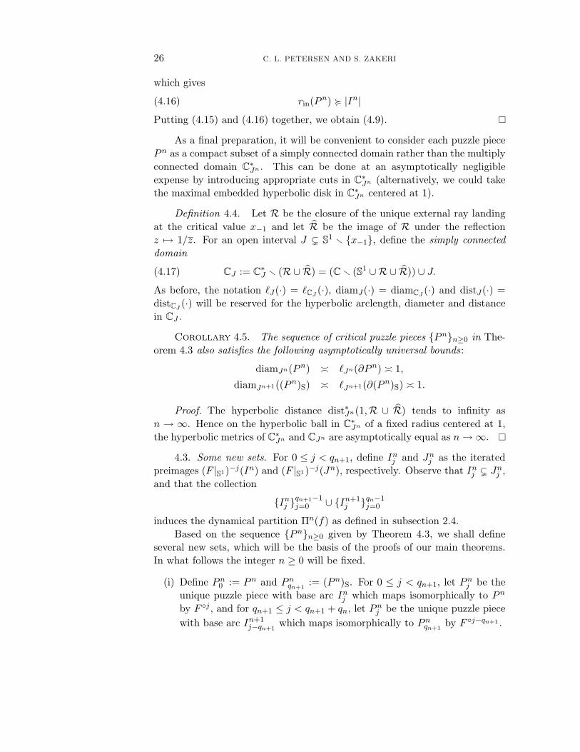
(ii) For 0 ≤ j < qn+1 +qn, we define the reflected puzzle piece Pnj ⊂ D as the
image of Pnj under z → 1/z. By abuse of the language, these reflected
puzzle pieces and their iterated F -preimages outside D will also be called“puzzle pieces”. To emphasize this distinction, the original elements ofthe dyadic puzzle will sometimes be referred to as the exterior puzzlepieces.
(iii) Let Qn0 ⊂ U0 be the unique puzzle piece which satisfies F (Qn
0 ) = f(Pnqn+1
)= Pn
qn+1−1. For 0 ≤ j < qn+1 + qn, define Qnj to be the unique puzzle
piece in Uj which maps isomorphically to Qn0 by F j . Similarly, for
0 ≤ j < qn+1 + qn, define Qnj ⊂ D to be the image of Qn
j under thereflection z → 1/z (see Figure 5).
(iv) For 0 ≤ j < qn+1 + qn, j = qn+1 − 1, let Pn0,j be the unique puzzle piece
whose base arc is on ∂U0 and satisfies F (Pn0,j) = Pn
j . Similarly, we definePn
0,j ⊂ U0 as the reflection of Pn0,j in ∂U0, i.e., the unique puzzle piece
with the same base arc as Pn0,j which satisfies F (Pn
0,j) = Pnj .
1
n
1-
1-
nq+1
P
,0x qn
Q
QP
xqn
P
Pxqn
nqU
qn
Uqn
x xqn+1 - 1xqn - 1
-
n +1
+1
U0
1
n0
0n
n0
n0
,
n
xP
+
qn+1 - 1qn+1
qn+1
x - 1nq
0
0 + qn- 1
x
q
, qn+1 1-
P +0 , nn + q
1
- 1
n
q+ + n
+1+ qn
2
Figure 5. Some other puzzle pieces.
(v) For 0 ≤ j < qn+1 + qn, let Qn0,j and Qn
0,j denote the unique puzzle piecescontaining x0,j which map by F to Qn
j and Qnj , respectively.
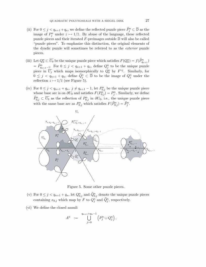
(vi) We define the closed annuli
An :=qn+1+qn−1⋃
j=0
(Pn
j ∪ Qnj
),
28 C. L. PETERSEN AND S. ZAKERI
An :=qn+1+qn−1⋃
j=0
(Pn
j ∪ Qnj
),
An := An ∪ An.
It is easy to check that An is a closed topological annulus whose interiorcontains the unit circle.
(vii) Similarly, we define the closed “rectangles”
An0 :=
qn+1+qn−1⋃j=0,j =qn+1−1
Pn0,j ∪
qn+1+qn−1⋃j=0
Qn0,j ,
An0 :=
qn+1+qn−1⋃j=0,j =qn+1−1
Pn0,j ∪
qn+1+qn−1⋃j=0
Qn0,j ,
An0 := An
0 ∪ An0 .
It is easy to check that An0 is a closed topological disk which does not
contain the critical point x0 = 1. Moreover, An ∪ An0 contains an open
neighborhood of the union S1 ∪ ∂U0 (see Figure 6). Note also thatF−1(An) ∩ U0 = An
0 ∪ Qn0 .
An
An ∩ An0
An0
Figure 6. Schematic picture of the annulus An and the “rectangle” An0 .
(viii) Finally, pull these annuli and rectangles back to define the sets
Zn−1 := An, Zn
k := An ∪k⋃
m=0
F−m(An0 ∪ Qn
0 ),
Zn := An ∪∞⋃
m=0
F−m(An0 ∪ Qn
0 ),
Yn−1 := An, Yn
k := An ∪k⋃
m=0
F−m(An0 ), Yn := An ∪
∞⋃m=0
F−m(An0 ).
QUADRATIC POLYNOMIALS WITH A SIEGEL DISK 29
Observe that Znk and Zn = limk→∞Zn
k are subsets of the filled Julia setK(F ). Moreover, we have the inclusions
Zn+2k ⊂ Zn
k , Yn+2k ⊂ Yn
k , Znk ⊂ Yn
k
Zn+2 ⊂ Zn, Yn+2 ⊂ Yn, Zn ⊂ Yn.
In what follows we use the generic symbol P for any of the puzzle piecesP or Q defined in the items (i)–(v) above, as well as their iterated preimagesunder F . Similarly, the generic symbol P will be used for any of the puzzlepieces P or Q defined in (i)–(v) and their preimages. Note that puzzle piecesalways come in pairs (P, P ) which are the reflections of one another throughthe boundary of some drop U , with P ∩ U = ∅, and P ⊂ U .
By an abuse of language, we say that a puzzle piece P belongs to one ofthe sets defined in items (vi)–(viii) above if P appears as a puzzle piece inone of the unions used in the definition of that set. We use the notation toexpress this relation. As an example, Pn
0 belongs to An and we write Pn0 An.
Note that the relation implies the set-theoretic ⊂, but not vice versa. Forinstance, Pn+2
0 ⊂ Zn but Pn+20 Zn does not hold.
4.4. Supporting lemmas. This subsection will prove several a priori es-timates on the geometry of the puzzle pieces and the sets defined above. Asis common in dynamics, distortion estimates for long compositions of f or itsinverse play a central role. We use the following version of the classical Koebedistortion theorem (see for example [Po]):
Theorem 4.6. Let φ : U → C be a univalent map on a simply-connecteddomain U C and let K ⊂ U be compact with hyperbolic diameter d. Then
χ(φ, K) := sup∣∣∣∣ φ′(z)
φ′(w)
∣∣∣∣ : z, w ∈ K
≤ e4d.
Lemma 4.7. The following asymptotically universal bounds exist :
diamJn0(Pn
0 ) = diamJn0(Pn
0 ) 1,
diamJn+10
(Pnqn+1
) = diamJn+10
(Pnqn+1
) 1,
diamJn0(Qn
0 ) = diamJn0(Qn
0 ) 1.
Proof. The first two come from Corollary 4.5. To prove the third bound,observe that diam(Pn
qn+1) diam(Qn
0 ) and hence by the second bound we havethe (Euclidean) asymptotically universal bound
|Jn0 | |Jn+1
0 | diam(Pnqn+1
) diam(Qn0 ).
Since Qn0 is a subset of U0 whose boundary makes an angle of π/3 with the
unit circle at z = 1, the third bound follows.
30 C. L. PETERSEN AND S. ZAKERI
Combining Lemma 4.7 with Theorem 4.6, we immediately obtain
Corollary 4.8. Let g be any univalent branch of f−k defined on thesimply connected domain CJn
0. Then, there exist the asymptotically universal
distortion bounds
χ(g, Pn0 ∪ Pn
0 ) χ(g, Pn−1qn
∪ Pn−1qn
) χ(g, Qn0 ∪ Qn
0 ) 1
uniformly in g.
Lemma 4.9. There exists the following asymptotically universal bound :
area(Pn0 ) |In|2.
Proof. This is an immediate consequence of (4.9) in Theorem 4.3 and thefact that ∂U0 makes an angle of π/3 with S1 at 1.
Lemma 4.10. There exist the following asymptotically universal bounds:
area(Pn0 An+2) area(Pn
0 An+2) area(Pn0 ∪ Pn
0 ),
area(Pnqn+1
An+2) area(Pnqn+1
An+2) area(Pnqn+1
∪ Pnqn+1
),
area(Qn0 An+2) area(Qn
0 An+2) area(Qn0 ∪ Qn
0 ).
Proof. We prove the first bound, the other two being similar. Clearly,
area(Pn0 An+2) area(Pn
0 An+2) area(Pn0 ∪ Pn
0 ),
and so we need only prove the reverse bound. With i = qn + qn−1−1, the basearc of the puzzle piece Pn+2
0,i satisfies I(Pn+20,i ) = [x0,i+qn+2 , x0,i] ⊂ [1, x0,i] =
O(Pn). It follows that Pn+20,i ⊂ Pn
0 An+2 (see Figure 5). Observe that by reala priori bounds, Corollary 4.8 and Lemma 4.9,
|In|2 |[xqn+2+qn+qn−1 , xqn+qn−1 ]|2
|[x0,qn+2+i, x0,i]|2 = |I(Pn+20,i )|2
area(Pn+20,i ).
Hence by another application of Lemma 4.9,
area(Pn0 ∪ Pn
0 ) |In|2 area(Pn+20,i ).
Since area(Pn0 An+2) ≥ area(Pn+2
0,i ), we obtain the reverse bound
area(Pn0 An+2) area(Pn
0 ∪ Pn0 ).
QUADRATIC POLYNOMIALS WITH A SIEGEL DISK 31
Our next task is to estimate the area of the sets Zn and Yn defined above.We use Corollary 4.8 to prove two distortion lemmas which will be essential inthe proof of Theorem 4.15. The first lemma deals with the pull-backs of thecritical puzzle pieces to An and An
0 only:
Lemma 4.11. Every pair (P, P ) An or An0 is a bounded distortion pull -
back of the corresponding pair of critical puzzle pieces in An. More precisely,let g be the univalent branch of f−j which maps the pair of critical puzzlepieces (P ′, P ′) An to (P, P ), where (P ′, P ′) = (Pn
0 , Pn0 ) or (Pn
qn+1, Pn
qn+1) or
(Qn0 , Qn
0 ). Thenχ(g, P ′ ∪ P ′) 1
uniformly in g.
Proof. Let us first assume (P, P ) An. It suffices to consider the case(P, P ) = (Pn
j , Pnj ) for some 0 ≤ j < qn+1, because the other two cases are
similar. The critical values of fj are located at 0,∞, x−1, . . . , x−j , none ofwhich belongs to CJn
0since j < qn+1. Hence the univalent branch g = f−j
which maps Pn0 ∪ Pn
0 to Pnj ∪ Pn
j extends univalently to the simply-connecteddomain CJn
0, and the claim follows from Corollary 4.8.
Now let us assume (P, P ) An0 . Then either (P, P ) = (Pn
0,j , Pn0,j) for
some 0 ≤ j < qn+1 − 1, or for some qn+1 − 1 < j < qn+1 + qn, or else(P, P ) = (Qn
0,j , Qn0,j) for some 0 ≤ j < qn+1 + qn. Again, let us consider only
the first case, the others being similar. In this case, the branch g = f−j−1
which maps Pn0 ∪ Pn
0 to Pn0,j ∪ Pn
0,j has a univalent extension to CJn0
since byj + 1 < qn+1 the latter set does not contain any critical value of fj+1. Hence,again, the claim follows from Corollary 4.8.
The second distortion lemma considers further pull-backs of puzzle pieces.First, it will be convenient to include the following:
Definition 4.12. For an integer k ≥ 0 and a k-drop U , consider thebranch of f−k = F−k mapping U0 isomorphically to U . It is easy to seethat this branch has a univalent extension to the simply connected domainC (D ∪R), where R is the closure of the external ray landing at the criticalvalue x−1. We denote this univalent extension by gU . Furthermore, we define
Hk := gU : U is a drop of depth k,and we set H :=
⋃∞k=0 Hk. Note that H0 = id.
Lemma 4.13. For every pair of puzzle pieces (P, P ) An0 , there exists the
asymptotically universal distortion bound
χ(g, P ∪ P ) 1
which holds uniformly in (P, P ) and g ∈ H.
32 C. L. PETERSEN AND S. ZAKERI
Proof. Note that every g ∈ H is defined on An0 since the domain C(D∪R)
certainly contains An0 . Fix a pair (P, P ) An
0 . By the proof of Lemma 4.11,the univalent branch g1 of f−j−1 which maps the pair of critical puzzle pieces(P ′, P ′) An to (P, P ) has a univalent extension to CJn
0or CJn+1
0(depending
on which of the three possible types (P ′, P ′) is). Let us assume we have thefirst case, the other two cases being similar. If Ω := g1(CJn
0), it follows that the
hyperbolic diameter diamΩ(P ∪ P ) is equal to diamJn0(P ′∪ P ′) which is 1 by
Lemma 4.7. Let Ω′ be the connected component of Ω (D∪R) containing thepair (P, P ). It is easy to see that Ω′ is simply connected and diamΩ′(P∪P ) 1.It follows that g is univalent in Ω′ and Theorem 4.6 implies χ(g, P ∪ P ) 1 asclaimed.
Lemma 4.14. (i) Let k ≥ 0, U be a k-drop, P ′ be an exterior puzzle piece,and n ≥ 0. If U ∩ P ′ = ∅, then U ⊂ P ′ and gU (An
0 ) ⊂ P ′.
(ii) Let k ≥ 0 and U be a k-drop. Then either gU (An0 ) ⊂ Yn
k−1 or gU (An0 ) ∩
Ynk−1 = ∅.
(iii) For every k ≥ 0, there is the equality
Ynk = Yn
k−1 ∪⋃
P ∪ P : P Hk(An0 ) and P ∩ Yn
k−1 = ∅.
(iv) For every P Hk(An0 ) with P ∩ Yn
k−1 = ∅, P Yn+2k = P Zn+2
k .
Proof. (i) As was remarked in subsection 4.1, U ∩ P ′ = ∅ implies U ⊂ P ′
so that P ⊂ P ′ for every P gU (An0 ). If P gU (An
0 ), then the interior of P
intersects the interior of P ′ since P ′ contains a neighborhood of U x(U).It follows from the nested property of puzzle-pieces that P ⊂ P ′.
(ii) For k = 0 the claim is clear since An0 ∩ Yn
−1 = ∅. Assume k ≥ 1 andconsider a k-drop U . If gU (An
0 ) ∩ Ynk−1 = ∅, then for some external puzzle
piece P ′ Ynk−1 we must have U ∩ P ′ = ∅. It follows from (i) that U ⊂ P ′ and
gU (An0 ) ⊂ P ′. This proves gU (An
0 ) ⊂ Ynk−1.
(iii) From the definition Ynk = Yn
k−1 ∪ Hk(An0 ). Hence the inclusion ⊃
is trivial. For the reverse inclusion, suppose that z ∈ Ynk Yn
k−1. Then z ∈Hk(An
0 ), which means z ∈ P ∪ P , where P gU (An0 ) for some k-drop U .
Since z ∈ gU (An0 ) Yn
k−1, by (ii) we must have gU (An0 ) ∩ Yn
k−1 = ∅, so thatP ∩ Yn
k−1 = ∅.(iv) As P ∩ Yn
k−1 = ∅ implies P ∩ Yn+2k−1 = ∅,
P Yn+2k = P Hk(An+2
0 ) = P Hk(An+20 ∪ Qn+2
0 ) = P Zn+2k ,
where the last equality holds since P ∩ Zn+2k−1 = ∅.
QUADRATIC POLYNOMIALS WITH A SIEGEL DISK 33
The following is one of the main technical results of this paper. It isthis estimate which allows us to show that the pull-back of a David-Beltramidifferential on D to the union of all drops is a David-Beltrami differential on C(compare Theorem B).
Theorem 4.15. The following asymptotically universal bound exists:
(4.18) area(Yn Yn+2) area(Yn).
As a result, there is a universal constant 0 < δ < 1 such that
(4.19) area(Zn) ≤ area(Yn)δn.
Proof. Combining Lemma 4.10 with Lemma 4.11, we obtain a universalconstant 0 < λ′ < 1 and an integer N ′ ≥ 1 such that for every n ≥ N ′,
(4.20)area(P An+2) ≥ λ′ area(P ∪ P ) for all P An,
area(P An+20 ) ≥ λ′ area(P ∪ P ) for all P An
0 .
This, together with Lemma 4.13, shows that there exist a universal constantλ and an integer N , with 0 < λ < λ′ < 1 and N ≥ N ′, such that for everyn ≥ N , k ≥ 0, and P Hk(An
0 ),
(4.21) area(P Zn+2k ) ≥ λ area(P ∪ P ).
We shall prove by induction on k ≥ −1 that for every n ≥ N ,
(4.22) area(Znk Yn+2
k ) ≥ λ area(Ynk ).
For the induction basis, note that the puzzle pieces which belong to An havedisjoint interiors. Thus, summing up the first estimate in (4.20) over all P An,we obtain
area(Zn−1 Yn+2
−1 ) = area(Zn−1 Zn+2
−1 ) ≥ λ′ area(An) > λ area(Yn−1).
For the induction step, assume (4.22) holds for some k − 1 ≥ −1. WritingZn
k = Znk−1 ∪Hk(An
0 ∪Qn0 ), we have the following estimates in which the sums
are taken over all puzzle pieces P Hk(An0 ) which do not intersect Yn
k−1:
area(Znk Yn+2
k ) ≥ area(Znk−1 Yn+2
k ) +∑P
area(P Yn+2k )
(by Lemma 4.14(iv)) = area(Znk−1 Yn+2
k−1 ) +∑P
area(P Zn+2k )
(by (4.21) and (4.22)) ≥ λ area(Ynk−1) +
∑P
λ area(P ∪ P )
(by Lemma 4.14(iii)) ≥ λ area(Ynk ).
34 C. L. PETERSEN AND S. ZAKERI
This completes the induction step. It now follows from (4.22) that for everyk ≥ −1 and n ≥ N ,
area(Yn Yn+2k ) ≥ area(Yn
k Yn+2k ) ≥ area(Zn
k Yn+2k ) ≥ λ area(Yn
k ).
Taking the limit as k → ∞ yields area(Yn Yn+2) ≥ λ area(Yn), which isequivalent to (4.18).
The proof of (4.19) is now immediate. Let 0 < η := 1 − λ < 1 and let N
be as above. Then by induction we obtain
area(Yn) ≤ ηn−N−1
2 area(Y1) ≤ ηn−N−1
2 areaz : G(z) ≤ 1,where G : A(∞) → R is the Green’s function on the basin of infinity. Sincethis last area is bounded by a universal constant C > 0, we obtain
area(Yn) ≤ C ηn3
for all n ≥ 3N + 3, which proves (4.19) with δ := η13 .
5. Proofs of Theorems A and B
In this section we prove Theorems A and B cited in the introduction. Asindicated there, Theorem B implies that a David-Beltrami differential sup-ported on D extends to an F -invariant David-Beltrami differential on C bypull-back. Note that the statement of this theorem is completely independentof the arithmetic of the rotation number θ. Thus, with Theorem B in hand, itfollows that Theorem A is true for any arithmetical condition on θ for whichthe more elementary Theorem C holds (compare Questions 1 and 2 in theintroduction and the discussion there).
5.1. Concentrating Lebesgue measure. Consider the Blaschke productf = fθ of (3.1) and the modified map F = Fθ,H of (3.2) for any irrational0 < θ < 1 and any homeomorphism H. We will associate to f a measureν = νθ depending only on θ, supported on the closed unit disk and with totalmass equal to area(K(F )). This measure is obtained by summing up the pushforward of Lebesgue measure on each drop U by the minimal iterate of f map-ping U to D. More explicitly, let g0 : D → U0 denote the univalent branch off−1 = F−1 and let H be as in Definition 4.12. Then, for any measurable setE ⊂ D,
(5.1) ν(E) := area(E) +∑g∈H
area(g g0(E)).
Evidently ν is absolutely continuous with respect to Lebesgue measure on Dso that ν(E) → 0 as area(E) → 0. Remarkably, it is possible to control therate of this convergence by the following power law:
QUADRATIC POLYNOMIALS WITH A SIEGEL DISK 35
Theorem B. The measure ν = νθ is dominated by a universal power ofLebesgue measure. In other words, there exist a universal constant 0 < β < 1and a constant C > 0 (depending on θ) such that
ν(E) ≤ C (area(E))β
for every measurable set E ⊂ D.
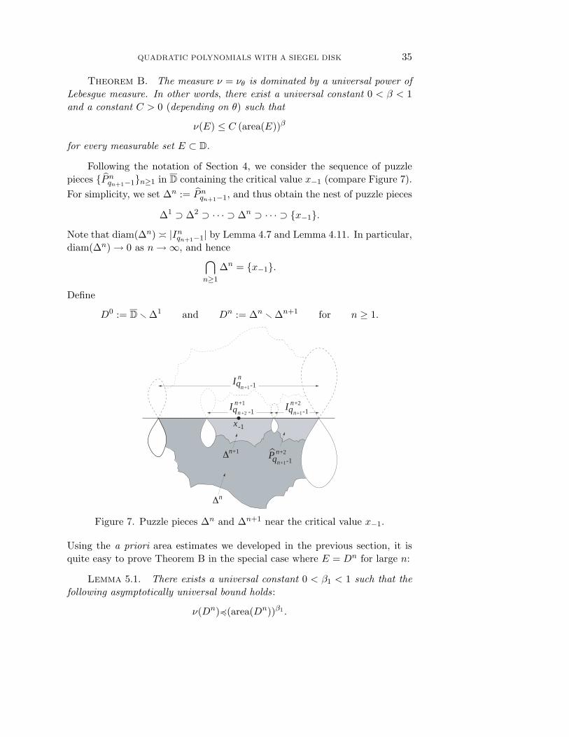
Following the notation of Section 4, we consider the sequence of puzzlepieces Pn
qn+1−1n≥1 in D containing the critical value x−1 (compare Figure 7).For simplicity, we set ∆n := Pn
qn+1−1, and thus obtain the nest of puzzle pieces
∆1 ⊃ ∆2 ⊃ · · · ⊃ ∆n ⊃ · · · ⊃ x−1.
Note that diam(∆n) |Inqn+1−1| by Lemma 4.7 and Lemma 4.11. In particular,
diam(∆n) → 0 as n → ∞, and hence⋂n≥1
∆n = x−1.
Define
D0 := D ∆1 and Dn := ∆n ∆n+1 for n ≥ 1.
+2
+1
+1nqn
-1
+1nq+2n
n +1
n-1nq
+2n
-1
-1
q
n∆
I
∆n P+1
-1x
I
I
Figure 7. Puzzle pieces ∆n and ∆n+1 near the critical value x−1.
Using the a priori area estimates we developed in the previous section, it isquite easy to prove Theorem B in the special case where E = Dn for large n:
Lemma 5.1. There exists a universal constant 0 < β1 < 1 such that thefollowing asymptotically universal bound holds:
ν(Dn)(area(Dn))β1 .
36 C. L. PETERSEN AND S. ZAKERI
Proof. SinceDn ∪
⋃g∈H
g g0(Dn) ⊂ Zn
for all n ≥ 1, it follows from (5.1) and Theorem 4.15 that
(5.2) ν(Dn) ≤ area(Zn) ≤ area(Yn) δn.
We claim thatarea(Dn) area(∆n).
In fact, In+2qn+1−1 and In+1
qn+2−1 are interiorly disjoint subintervals of Inqn+1−1, and
by Theorem 2.5|In+2
qn+1−1| |In+1qn+2−1| |In
qn+1−1|.
It follows in particular that Pn+2qn+1−1 ⊂ Dn (compare Figure 7). By Lemma 4.9
and Lemma 4.11,
area(∆n) ≥ area(Dn) ≥ area(Pn+2qn+1−1) |In+2
qn+1−1|2 |Inqn+1−1|2 area(∆n),
which proves our claim. It follows that
(5.3) area(Dn) area(∆n) |Inqn+1−1|2 σ6n
1 ,
where 0 < σ1 < 1 is the universal constant given by Lemma 2.7. Now by(5.2) and (5.3), any positive constant β1 < (log δ)/(6 log σ1) will satisfy thecondition of the lemma.
Lemma 5.2. There exists the following asymptotically universal bound :
dist(x−1, ∂Pnqn+1−1 S1) |In
qn+1−1|.
Proof. Note that
Pnqn+1−1 = f(Pn
qn+1) = f((Pn)S).
For any w ∈ ∂Pnqn+1−1 S1 there is a unique z in the union B∪R∪G ⊂ ∂(Pn)S
such that w = f(z). Since f has a cubic critical point at 1, it follows from(4.10) in Theorem 4.3 that
|x−1 − w| |1 − z| 13 |In+1| 13 |Inqn+1−1|.
Corollary 5.3. Let T := rx−1 : r ≥ 1 be the radial line segment goingfrom the critical value out to infinity. Then there is the following asymptoticallyuniversal bound :
diamCT (Dn) 1.
Proof. This easily follows from the above Lemma 5.2 since Dn =∆n ∆n+1, |In
qn+1−1| |In+1qn+2−1|, and the hyperbolic metric of C T at z
is comparable to 1/ dist(z, T ).
QUADRATIC POLYNOMIALS WITH A SIEGEL DISK 37
Let W denote the connected component of F−1(C T ) which contains U0.Then W ⊂ C D and g0 extends to a biholomorphic map g0 : C T → W .Hence each g g0 for g ∈ H has a univalent extension to C T and we obtainthe following result by applying Theorem 4.6 and Corollary 5.3:
Corollary 5.4. There exists the asymptotically universal distortionbound
χ(g g0, Dn) 1,
which holds uniformly in g ∈ H.
Proof of Theorem B. Choose positive constants C1, C2 and C3 (all de-pending on θ), such that for all n ≥ 0 and all g ∈ H,
ν(Dn) ≤ C1 (area(Dn))β1 ,
χ(g g0, Dn) ≤ C2,
area(Dn) ≤ C3 δn.
The existence of these constants is assured by Lemma 5.1, Corollary 5.4 andthe estimate (5.2), respectively. Fix a measurable set E ⊂ D and decomposeit into the disjoint union
E = E0 ∪ E1 ∪ E2 ∪ · · · ,
where En := Dn ∩ E for n ≥ 0. Then,
ν(En) = area(En) +∑g∈H
area(g g0(En))
≤ C22
area(En)area(Dn)
area(Dn) +∑g∈H
area(g g0(Dn))
= C2
2
area(En)area(Dn)
ν(Dn)
= C22
ν(Dn)(area(Dn))β1
(area(En)area(Dn)
)1−β1
(area(En))β1 ,
which gives
(5.4) ν(En) ≤ C1 C22 (area(En))β1 for all n ≥ 0.
38 C. L. PETERSEN AND S. ZAKERI
Choose any 0 < β < β1 and let β2 := β1 − β. Then, it follows from (5.4) andHolder’s inequality that
ν(E) ≤ C1 C22
∞∑n=0
(area(En))β+β2
≤ C1 C22
( ∞∑n=0
(area(En))β2
1−β
)1−β ( ∞∑n=0
area(En)
)β
≤ C1 C22 Cβ2
3
( ∞∑n=0
δnβ21−β
)1−β
(area(E))β.
This completes the proof of Theorem B.
5.2. Main Theorem. Now we are ready to prove the main result of thiswork:
Theorem A. Let E denote the set of irrational numbers θ = [a1, a2, a3, . . .]which satisfy the arithmetical condition
log an = O(√
n) as n → ∞.
If θ ∈ E , then the Julia set of the quadratic polynomial Pθ : z → e2πiθz + z2 islocally connected and has Lebesgue measure zero. In particular, the Siegel disk∆θ of Pθ is a Jordan domain whose boundary contains the finite critical pointof Pθ.
Recall that E has full measure in [0, 1] by Corollary 2.2.
Proof. Fix an irrational θ ∈ E and consider the Blaschke product fθ in(3.1). By Theorem C (see the end of subsection 2.6 as well as the appendix),there exists a David homeomorphism H : D → D, with H fθ H−1 = Rθ onS1, so that
areaz ∈ D : |µH |(z) > 1 − ε ≤ M e−αε for all 0 < ε < ε0.
Here M > 0 is universal, α > 0 depends on lim supn→∞(log an)/√
n, and0 < ε0 < 1 depends on θ. Let F = Fθ,H denote the Blaschke map modified byH as in (3.2). We define an F -invariant measurable Beltrami differential µ onC as follows: First, on the unit disk D, let
µ := µH =∂H
∂H
dz
dz
be the pull-back of the zero Beltrami differential by H. Then, pull µ|D back tothe union of all drops by the univalent branches g g0 for g ∈ H. Finally, onthe rest of the plane, define µ to be the zero Beltrami differential. By the very
QUADRATIC POLYNOMIALS WITH A SIEGEL DISK 39
construction, F ∗(µ) = µ. Also, the branches g g0 used to spread µ aroundare all conformal, so they do not change |µ|. It follows that
areaz ∈ C : |µ|(z) > 1 − ε = νz ∈ D : |µ|(z) > 1 − ε,
where ν is the measure defined in (5.1). By Theorem B, there is a univer-sal constant 0 < β < 1 and a constant C > 0 depending on θ such thatν(E) ≤ C (area(E))β for all E ⊂ D. It follows that for all 0 < ε < ε0,
areaz ∈ C : |µ|(z) > 1−ε ≤ C (areaz ∈ D : |µ|(z) > 1 − ε)β ≤ C Mβ e−αβε .
One can actually get rid of the constants in front of the exponential by makingε0 smaller. In fact, choose any ω such that 0 < ω < α β and define
ε1 := min
ε0,α β − ω
log(C Mβ)
.
Then a brief computation shows that if 0 < ε < ε1,
(5.5) areaz ∈ C : |µ|(z) > 1 − ε ≤ e−ωε .
This shows that µ is a David-Beltrami differential, hence integrable by The-orem 2.8. Let ϕ : C → C be the solution to the Beltrami equation µϕ = µ,normalized by ϕ(H−1(0)) = 0, ϕ(1) = −e2πiθ/2. Let P := ϕ F ϕ−1 denotethe conjugate map. Assuming for a moment that P is a quadratic polynomial(see Lemma 5.5 below), we see clearly that ∆ = ϕ(D) is a Siegel disk of ro-tation number θ for P . By the way we normalized ϕ, we must have P = Pθ.Local connectivity of Jθ now follows from Theorem 3.1 and the fact that ϕ isa homeomorphism. That area(Jθ) = 0 follows from Theorems 3.2 and 2.9.
It remains to prove the following
Lemma 5.5. The conjugate map P := ϕ F ϕ−1 is a quadratic polyno-mial.
Note that this trivially follows from Weyl’s lemma when µ has boundeddilatation on C, or equivalently when ϕ is quasiconformal.
Proof. P is a degree 2 branched covering of the sphere with P−1(∞) = ∞,so it will be a quadratic polynomial once we show that it is holomorphic. Tothis end, we prove that ϕF ∈ W 1,1
loc (C1). Then, on a small neighborhood U
of every regular point of F , both ϕ and ϕF pull the zero Beltrami differentialback to µ|U , and it follows from Theorem 2.8 that they must coincide up to aconformal map, meaning in particular that P must be holomorphic in ϕ(U).This argument will show that P is holomorphic on C ϕ(1), hence on theentire plane.
So let us prove ϕ F ∈ W 1,1loc (C 1). Evidently ϕ F ∈ W 1,1
loc (C D)simply because F is holomorphic in C D and ϕ ∈ W 1,1
loc (C). On the other
40 C. L. PETERSEN AND S. ZAKERI
hand, on D we can write ϕF = ϕH−1Rθ H. Here ϕH−1 is conformal byanother application of Theorem 2.8 since both H and ϕ are homeomorphismsin W 1,1
loc (D) pulling the zero Beltrami differential back to µ|D. It follows thatϕ F is given in D by postcomposing H with a conformal map, hence is inW 1,1
loc (D).It remains to show that ϕ F ∈ W 1,1
loc (U) for every small open disk U
whose center belongs to S1 1. Note that by the above argument ϕ F isdifferentiable almost everywhere in U , which shows∫
UJac(ϕ F ) ≤ area((ϕ F )(U)) < +∞,
so that Jac(ϕ F ) ∈ L1(U). Moreover, on every compact subset of U S1 theordinary partial derivatives ∂(ϕ F ) and ∂(ϕ F ) are integrable and coincidewith the distributional derivatives of ϕF . If we show that ∂(ϕF ), and hence∂(ϕF ) = µϕF ∂(ϕF ), is in L1(U), it follows from a standard approximationargument that ∂(ϕ F ) and ∂(ϕ F ) are the distributional partial derivativesin U , and hence ϕ F ∈ W 1,1
loc (U). But ∂(ϕ F ) ∈ L1(U) is fairly easy to see:since µϕF = µ almost everywhere in U , we have
|∂(ϕ F )|2 =Jac(ϕ F )1 − |µϕF |2
≤ Jac(ϕ F )1 − |µϕF |
=Jac(ϕ F )
1 − |µ| ,
so that|∂(ϕ F )| ≤ Jac(ϕ F )
12 (1 − |µ|)−
12 .
By the exponential growth condition (5.5), the measurable function (1 − |µ|)−1
belongs to L1(C). It follows then from Holder inequality that ∂(ϕ F ) ∈L1(U).
We would like to draw the reader’s attention to the following corollarywhich is implicit in the above proof. It describes how the conjugating map inthe above construction depends on various parameters; this point may be ofinterest in possible future investigations, when one considers a family of suchDavid conjugacies as θ varies in E :
Corollary 5.6. Let θ ∈ E and let ϕ be the conjugating homeomorphismbetween Fθ and Pθ given by Theorem A. Then ϕ is a David homeomorphismon C so that its dilatation satisfies an exponential condition of the form (2.7).Moreover, the constant M in (2.7) can be chosen to be 1, but in general α
depends on lim supn→∞(log an)/√
n and ε0 depends on θ.
By [P5], the boundary of the Siegel disk of Pθ is a quasicircle containingthe critical point if and only if θ belongs to the class D2 of bounded typeirrational numbers.
QUADRATIC POLYNOMIALS WITH A SIEGEL DISK 41
Corollary 5.7. Let θ belong to the full measure set E D2. Then theboundary of the Siegel disk of the quadratic polynomial Pθ is a Jordan curve ofmeasure zero containing the critical point, but it is not a quasicircle.
As a final remark, let us briefly sketch how to generalize Theorem A to thecase of Siegel disks of higher periods (we assume familiarity with the theoryof polynomial-like maps). Let P : z → z2 + c be a quadratic polynomial witha Siegel disk ∆ of period n > 1 and rotation number θ ∈ E . Douady andHubbard proved that P is renormalizable, i.e., there exist open topologicaldisks U and V , with ∆ ⊂ U ⊂ U ⊂ V , such that P n|U : U → V is adegree 2 proper holomorphic map (compare [Z1, Th. 4.2]). According to [DH2],P n|U is a hybrid equivalent to the quadratic polynomial Pθ. In particular, the“little Julia set” J := ∂z ∈ U : P nk(z) ∈ U for all k ≥ 1 is quasiconformallyhomeomorphic to the Julia set Jθ. It follows from Theorem A that J is locallyconnected and has measure zero. From this, it is not hard to draw the sameconclusions for the “big Julia set” J(P ). The fact that local connectivity ofJ implies that of J(P ) is standard in renormalization theory (see for example[P3]). That J(P ) has measure zero follows from the general principle (see [Ly]or [Mc1]) that the orbit of almost every z ∈ J(P ) converges to the postcriticalset of P , which is the union ∂∆ ∪ · · · ∪ P n−1(∂∆) in this case. Thus, up to aset of measure zero, J(P ) =
⋃k≥0 P−k(J), which shows area(J(P )) = 0.
6. Appendix: A proof of Theorem C
In this appendix we present a proof of Theorem C, which is substantiallybased on Yoccoz’s work in the unpublished manuscript [Yo2]. The idea of theproof is to construct two combinatorially equivalent dynamically defined celldecompositions for the upper half-plane using the critical circle map and thecorresponding rigid rotation. The cells in these decompositions have boundedgeometry and are labelled by an integer, called their level. The closer thecell is chosen to the boundary of H, the higher its level and the smaller itsEuclidean diameter will be. The required extension quasiconformally mapseach cell of level n of the first decomposition to a unique cell of level n of thesecond decomposition, with the dilatation depending only on the (n + 1)-stterm an+1 of the continued fraction expansion of the rotation number θ. Thecell decompositions of bounded geometry, a fundamental inequality of Yoccoz(Theorem 6.6 below), and a construction of Strebel (Lemma 6.10 below) arethe main ingredients of the proof.
6.1. Two cell decompositions for the upper half -plane. As in subsection2.4, let f : T → T be a critical circle map with a critical point at 0 andirrational rotation number θ = [a1, a2, a3, . . .] with convergents pn/qn. We setxn := f−n(0) for all n ∈ Z.
42 C. L. PETERSEN AND S. ZAKERI
Consider the dynamical partition Πn(f) as defined in subsection 2.4. It iseasy to see that the collection of endpoints of the intervals in Πn(f) is preciselythe set xj : 0 ≤ j < qn+1 + qn. By Theorem 2.5, these points chop the circleup into comparable adjacent pieces. Unfortunately, this is not true for thecorresponding partition for the rigid rotation Rθ unless θ is of bounded type.To circumvent this problem in our forthcoming arguments, we choose a slightlydifferent partition as follows.
For every integer n ≥ 0, consider the collection of points
Qn := xj : 0 ≤ j < qn
on T, so that Q0 = 0. It is not hard to see that
T Qn =
⋃0≤j<qn−qn−1
]xj+qn−1 , xj [
∪ ⋃
0≤j<qn−1
]xj , xj+qn−qn−1 [
.
Thus xj and xk, with j < k, are adjacent in Qn if and only if either k = j+qn−1
and 0 ≤ j < qn − qn−1, or k = j + qn − qn−1 and 0 ≤ j < qn−1. It follows thatin the first case(6.1)
[xk, xj ] ∩Qn+1 = xk, xk+qn , xk+2qn , . . . , xk+(an+1−1)qn= xj+qn+1−qn , xj,
and in the second case
(6.2) [xj , xk] ∩Qn+1 = xj , xj+qn , xj+2qn , . . . , xj+an+1qn = xk+qn+1−qn , xk.
As a result, we see that xj and xk, with j < k, are adjacent in both Qn andQn+1 if and only if an+1 = 1, k = j + qn−1, and 0 ≤ j < qn − qn−1.
Using the canonical projection R → T = R/Z, we lift the set Qn to thetranslation-invariant set Qn := Qn + Z in R. By the above construction, forn ≥ 1, the closure of each interval in T Qn is either an interval or the unionof two adjacent intervals in Πn(f). Hence, by the lift to R, Theorem 2.5(ii)implies the following:
Lemma 6.1. Any two adjacent intervals in R Qn have lengths compa-rable up to a bound which is asymptotically universal. In other words,
max |I||J | : I, J are adjacent in R Qn
1.
For n ≥ 0 and x ∈ Qn, let
Mn(x) :=12(xr − x),
where xr and x are the points in Qn immediately to the right and left of x.Evidently, Mn(x) > Mn+1(x) unless xr and x are adjacent to x in Qn+1 also,
QUADRATIC POLYNOMIALS WITH A SIEGEL DISK 43
in which case Mn(x) = Mn+1(x). Observe that M0(x) = 1 for all x ∈ Q0 = Z.Define
zn(x) := x + i Mn(x) n ≥ 0, x ∈ Qn.
Using the sequence zn, we shall define an imbedded graph Γ in the upperhalf-plane H as follows: The vertices of Γ are the points zn(x) : n ≥ 0 and x ∈Qn. Note that zn(x) = zn+1(x) if and only if Mn(x) = Mn+1(x), in whichcase the corresponding vertex of Γ is doubly labelled. The edges of Γ are thevertical segments
[zn(x), zn+1(x)] : n ≥ 0 and x ∈ Qn with Mn(x) = Mn+1(x)
as well as the nonvertical segments
[zn(x), zn(y)] : n ≥ 0 and x, y are adjacent in Qn.
By a cell of Γ we mean the closure of any bounded connected component ofHΓ. Any cell γ of Γ is uniquely determined by a pair of adjacent points x < y
in Qn with the property that either Mn(x) = Mn+1(x) or Mn(y) = Mn+1(y).The integer n ≥ 0 will be called the level of γ, or we say that γ is an n-cell.The top of the n-cell γ is formed by the nonvertical edge [zn(x), zn(y)] whileits bottom is formed by the union of nonvertical edges
[zn+1(t0), zn+1(t1)] ∪ [zn+1(t1), zn+1(t2)] ∪ . . . ∪ [zn+1(tk−1), zn+1(tk)],
where the points x = t0 < t1 < . . . < tk = y form the intersection [x, y] ∩Qn+1. The sides of γ are formed by the vertical edge [zn(x), zn+1(x)] (whichcollapses to a single point if Mn(x) = Mn+1(x)) as well as [zn(y), zn+1(y)](which similarly collapses to a single point if Mn(y) = Mn+1(y)). If k = 1 sothat x, y are also adjacent in Qn+1, then γ is either a triangle or a trapezoid.Otherwise k ≥ 2 and by (6.1) or (6.2), γ is a (k + 3)-gon, where k is eitheran+1 or an+1 + 1.
Note that for m ≥ n, any m-cell γ is contained in the horizontal strip
z ∈ H : 0 ≤ Im(z) ≤ maxx∈Qn
Mn(x).
Hence, Lemma 2.7 implies the following
Lemma 6.2. Fix any integer n ≥ 0. Then the union of all the m-cells ofΓ for all m ≥ n is contained in a horizontal strip z ∈ H : 0 ≤ Im(z) ≤ whose height satisfies an asymptotically universal bound σn
2 , where 0 <
σ2 < 1 is the universal constant given by Lemma 2.7.
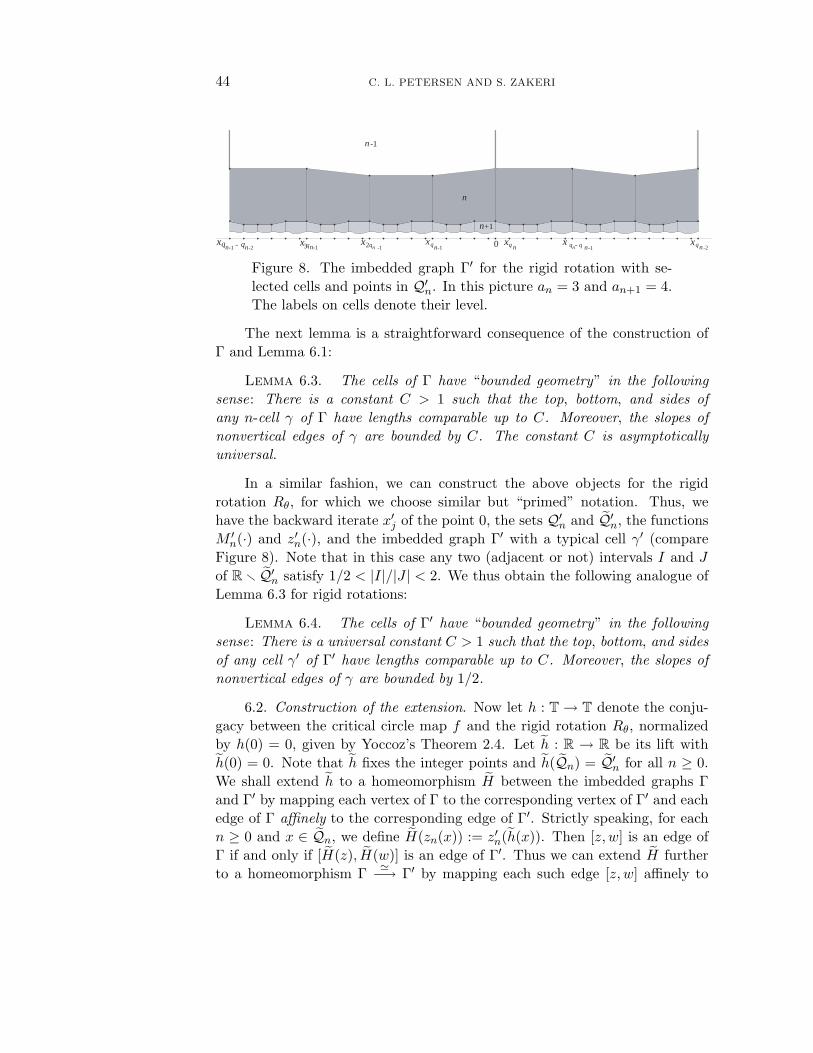
44 C. L. PETERSEN AND S. ZAKERI
-1x qn
xqn-1 - qn-2 3 xqn-1x qn -12 0 xq n
x qn- q n-1xqn -2
n
n+1
n -1
Figure 8. The imbedded graph Γ′ for the rigid rotation with se-lected cells and points in Q′
n. In this picture an = 3 and an+1 = 4.The labels on cells denote their level.
The next lemma is a straightforward consequence of the construction ofΓ and Lemma 6.1:
Lemma 6.3. The cells of Γ have “bounded geometry” in the followingsense: There is a constant C > 1 such that the top, bottom, and sides ofany n-cell γ of Γ have lengths comparable up to C. Moreover, the slopes ofnonvertical edges of γ are bounded by C. The constant C is asymptoticallyuniversal.
In a similar fashion, we can construct the above objects for the rigidrotation Rθ, for which we choose similar but “primed” notation. Thus, wehave the backward iterate x′
j of the point 0, the sets Q′n and Q′
n, the functionsM ′
n(·) and z′n(·), and the imbedded graph Γ′ with a typical cell γ′ (compareFigure 8). Note that in this case any two (adjacent or not) intervals I and J
of R Q′n satisfy 1/2 < |I|/|J | < 2. We thus obtain the following analogue of
Lemma 6.3 for rigid rotations:
Lemma 6.4. The cells of Γ′ have “bounded geometry” in the followingsense: There is a universal constant C > 1 such that the top, bottom, and sidesof any cell γ′ of Γ′ have lengths comparable up to C. Moreover, the slopes ofnonvertical edges of γ are bounded by 1/2.
6.2. Construction of the extension. Now let h : T → T denote the conju-gacy between the critical circle map f and the rigid rotation Rθ, normalizedby h(0) = 0, given by Yoccoz’s Theorem 2.4. Let h : R → R be its lift withh(0) = 0. Note that h fixes the integer points and h(Qn) = Q′
n for all n ≥ 0.We shall extend h to a homeomorphism H between the imbedded graphs Γand Γ′ by mapping each vertex of Γ to the corresponding vertex of Γ′ and eachedge of Γ affinely to the corresponding edge of Γ′. Strictly speaking, for eachn ≥ 0 and x ∈ Qn, we define H(zn(x)) := z′n(h(x)). Then [z, w] is an edge ofΓ if and only if [H(z), H(w)] is an edge of Γ′. Thus we can extend H furtherto a homeomorphism Γ −→ Γ′ by mapping each such edge [z, w] affinely to
QUADRATIC POLYNOMIALS WITH A SIEGEL DISK 45
[H(z), H(w)]. Note that H defined this way is the identity on the horizontalline R + i so that we can define H(z) = z for all z ∈ H with Im(z) ≥ 1. Itis easy to check that for each cell γ of Γ, the boundary ∂γ is mapped by H
homeomorphically and edgewise affinely onto the boundary ∂γ′ of a uniquecell γ′ of Γ′.
The following is the key result of this appendix:
Theorem 6.5 (Yoccoz). There exists a constant C > 0 with the followingproperty : For any n-cell γ of Γ, the edgewise affine boundary homeomorphismH : ∂γ → ∂γ′ extends to a quasiconformal homeomorphism H : γ → γ′ whosedilatation is at most C(1 + (log an+1)2). The constant C is asymptoticallyuniversal.
Assuming this result for a moment, we show how Theorem C, cited at theend of subsection 2.6, follows:
Proof of Theorem C. Consider the extension H : H → H obtained by glu-ing various extensions to cells given by Theorem 6.5. Clearly H is in W 1,1
loc (H)and satisfies H(z + 1) = H(z) + 1 for all z ∈ H. Since log an = O(
√n) by
the assumption, there are a constant C1 > 0 and an integer N1 ≥ 1, bothdepending on θ, such that 1 + (log an+1)2 ≤ C1 n whenever n > N1. By Theo-rem 6.5, there is a universal constant C2 > 0 and an integer N2 ≥ 1 dependingon f such that the dilatation K
Hin the interior of any n-cell of Γ is at most
C2 (1 + (log an+1)2) whenever n > N2. Finally, by Lemma 6.2, there is a uni-versal constant C3 > 0 and an integer N3 ≥ 1 depending on f such that ifn > N3,
∞⋃m=n
γ : γ is an m−cell of Γ ⊂ z ∈ H : 0 < Im(z) ≤ C3σn2 .
Set N := maxN1, N2, N3 and define
K0 := maxKH
(z) : z belongs to the interior of an m-cell of Γ with m ≤ N.
If KH
(z) > K > K0, then either z ∈ Γ (which has Lebesgue measure zero),or else z belongs to the interior of an n-cell of Γ with n ≥ N , so that K <
KH
(z) ≤ C1C2 n, or equivalently, n > K/(C1C2). It follows that
areaz ∈ H : 0 ≤ Re(z) ≤ 1 and KH
(z) > K ≤ C3 σK
C1C22 = C3 e
− log σ2C1C2
K.
The exponential map z → e2πiz does not change the dilatation and has normof the derivative bounded by 2π when restricted to the upper half-plane H.Therefore, the induced homeomorphism H : D → D satisfies
areaz ∈ D : KH(z) > K ≤ 4π2 C3 e− log σ2
C1C2K
46 C. L. PETERSEN AND S. ZAKERI
whenever K > K0. It follows that H is a David homeomorphism as in(2.8), with M = 4π2C3, α = (log σ2)/(C1C2), and K0 defined as above.Moreover, M is universal, α depends on C1 (which in turn depends onlim supn→∞(log an)/
√n), and K0 depends on f .
6.3. The proof of Yoccoz ’s theorem. It remains to give the proof of Theo-rem 6.5. Before we proceed, some preliminaries are in order.
Let n ≥ 1 and x, y be adjacent points in Qn. Let x = t0, t1, . . . , tk−1,
tk = y = [x, y] ∩ Qn+1. Note that by (6.1) and (6.2), k = an+1 or an+1 + 1.By Lemma 6.1, we know that each interval [tj−1, tj ] in this cascade has lengthcomparable to the next one [tj , tj+1]. However, for large values of k, the actionof fqn on this cascade of intervals is uniformly close to the action of a Mobiustransformation on its fundamental domains near a parabolic fixed point. Thisidea led Yoccoz to the following much sharper statement about the relativesize of these intervals, a proof of which can be found in [Yo2] or [dFdM]:
Theorem 6.6 (Yoccoz’s almost-parabolic bound). The lengths of theintervals in the above cascade satisfy
|[tj−1, tj ]| |[t0, tk]|
minj, k − j + 12
uniformly in j, 1 ≤ j ≤ k.
Mobius transformations with two distinct fixed points on the real line willplay a basic role in the proof of Theorem 6.5. For our purposes, it will beconvenient to put them in the normal form
(6.3) ζa(z) :=z
a − (a − 1)z, a ≥ 2, z ∈ C.
Note that ζa preserves the real line, has an attracting fixed point at z = 0 withmultiplier Dζa(0) = a−1 and a repelling fixed point at z = 1 with multiplierDζa(1) = a. (Here and in what follows, D is the differentiation operator.)
Lemma 6.7. The derivative Dζa(x) is monotonically increasing from 1/a
to a on 0 ≤ x ≤ 1. Moreover, for 0 ≤ x < x + ε ≤ 1, there exist the estimates
1 <Dζa(x + ε)
Dζa(x)≤ (1 + εa)2,
ε3a
(1 + εa)21
(1 − x)2≤ ζa(x + ε) − ζa(x) ≤ ε(1 + εa)2
a
1(1 − x)2
.
In particular, if ε is comparable to 1/a so that 1/(Ca) ≤ ε ≤ C/a for some
QUADRATIC POLYNOMIALS WITH A SIEGEL DISK 47
C ≥ 1, then the above estimates take the form
(6.4) 1 <Dζa(x + ε)
Dζa(x)≤ (1 + C)2,
(6.5)1
C3(1 + C)21
a2(1 − x)2≤ ζa(x + ε) − ζa(x) ≤ C(1 + C)2
1a2(1 − x)2
.
Proof. This is an elementary computation which will be left to the reader.For the second set of inequalities, it is convenient to estimate Dζa and applythe Mean Value Theorem.
Finally, let us also recall the following standard result in quasiconformaltheory:
Lemma 6.8. Let K > 1 and g : R → R be a piecewise differentiablehomeomorphism such that
1K
≤ Dg(x) ≤ K
for all x at which g is differentiable. Then the homeomorphic extension G :H → H given by G(x + iy) := g(x) + iy is K-quasiconformal.
The proof of Theorem 6.5 begins as follows. Throughout we may assumek ≥ 4, for otherwise γ and γ′ are m-gons of bounded geometry for some m ≤ 6(compare Lemmas 6.3 and 6.4) and evidently there is an extension H : γ → γ′
with asymptotically universal dilatation. It will be convenient to normalizeboth γ and γ′ by mapping them to the upper half-plane. Let H = H∪R∪∞and R = R ∪ ∞. As before, let the projections on R of the vertices of then-cells γ and γ′ consist of the points
t0 < t1 < . . . < tk and t′0 < t′1 < . . . < t′k,
where t′j = h(tj). Since k ≥ 4, we have Mn(t0) = Mn+1(t0) and Mn(tk) =Mn+1(tk). It follows from Lemma 6.3 that the top of γ is bounded by thegraph of a positive affine map g1, with |Dg1| 1. The bottom of γ is boundedby the graph of a positive piecewise affine map g2 with |Dg2| 1. Moreover,
supt0≤x≤tk
g1(x) − g2(x) inft0≤x≤tk
g1(x) − g2(x) tk − t0.
Define a homeomorphism p : γ−→ SQ := x + iy : |x| ≤ 1 and 0 ≤ y ≤ 2 by
p(x, y) :=(−1 + 2
x − t0tk − t0
, 2y − g2(x)
g1(x) − g2(x)
).
Note that p is affine in the x-coordinate, is fiberwise affine in the y-coordinate,and maps the corners zn(t0), zn(tk), zn+1(t0) and zn+1(tk) to −1+2i, 1+2i, −1
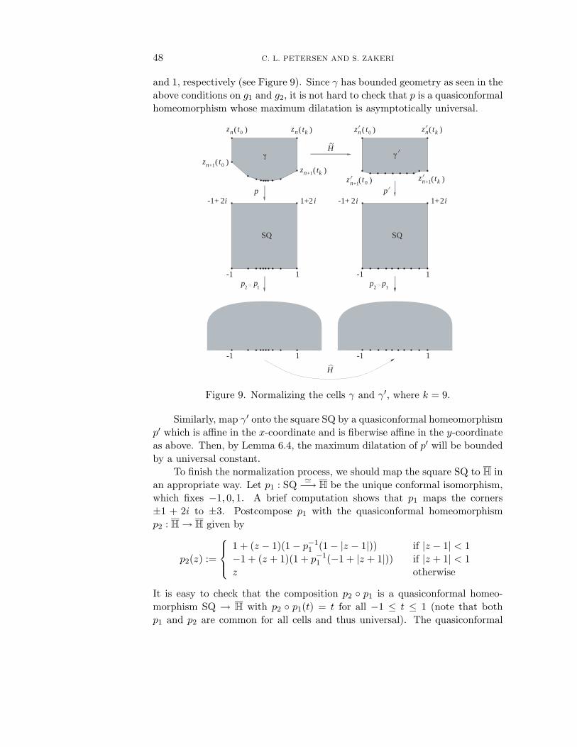
48 C. L. PETERSEN AND S. ZAKERI
and 1, respectively (see Figure 9). Since γ has bounded geometry as seen in theabove conditions on g1 and g2, it is not hard to check that p is a quasiconformalhomeomorphism whose maximum dilatation is asymptotically universal.
p
SQ
p
H
p2
p1 1
p2
p
H
-1 1 -1 1
1-11-1
i i
( )+1nz t( )n+1z t
( )nz t ( )nz t
+1( )zn t zn+1( )t
( )nz t0
0
0
0 k
k
k
( )nz tk
~
2-1+ 1+2 i 2-1+ 1+ i2
SQ
γ γ
Figure 9. Normalizing the cells γ and γ′, where k = 9.
Similarly, map γ′ onto the square SQ by a quasiconformal homeomorphismp′ which is affine in the x-coordinate and is fiberwise affine in the y-coordinateas above. Then, by Lemma 6.4, the maximum dilatation of p′ will be boundedby a universal constant.
To finish the normalization process, we should map the square SQ to H inan appropriate way. Let p1 : SQ −→ H be the unique conformal isomorphism,which fixes −1, 0, 1. A brief computation shows that p1 maps the corners±1 + 2i to ±3. Postcompose p1 with the quasiconformal homeomorphismp2 : H → H given by
p2(z) :=
1 + (z − 1)(1 − p−1
1 (1 − |z − 1|)) if |z − 1| < 1−1 + (z + 1)(1 + p−1
1 (−1 + |z + 1|)) if |z + 1| < 1z otherwise
It is easy to check that the composition p2 p1 is a quasiconformal homeo-morphism SQ → H with p2 p1(t) = t for all −1 ≤ t ≤ 1 (note that bothp1 and p2 are common for all cells and thus universal). The quasiconformal
QUADRATIC POLYNOMIALS WITH A SIEGEL DISK 49
homeomorphisms
φ := p2 p1 p : γ → H and φ′ := p2 p1 p′ : γ′ → H
have maximum dilatations which are asymptotically universal and universal,respectively. They give the required normalizations of γ and γ′.
Define a new homeomorphism H := φ′ H φ−1 : R → R, and setsj := φ(zn+1(tj)), s′j := φ′(z′n+1(t
′j)) = H(sj). Note that H is the identity
when |x| ≥ 1, and maps the interval [sj−1, sj ] affinely onto the interval [s′j−1, s′j ]
for every 1 ≤ j ≤ k. From its definition, it is easy to see that the mapφ zn+1 : [t0, tk] → [−1, 1] sending tj to sj is affine. Together withTheorem 6.6, this shows the existence of an asymptotically universal constantC0 > 1 such that for every 1 ≤ j ≤ k,
(6.6)1
C0 minj, k − j + 12≤ sj − sj−1 ≤ C0
minj, k − j + 12.
Similarly, the map φ′ z′n+1 : [t′0, t′k] → [−1, 1] sending t′j to s′j is affine.
Together with the fact that the t′j are roughly equally spaced, this shows theexistence of a universal constant C1 > 1 such that for every 1 ≤ j ≤ k,
(6.7)1
C1 k≤ s′j − s′j−1 ≤ C1
k,
so that
(6.8)j
C1k≤ s′j + 1 ≤ C1j
kand
k − j
C1k≤ 1 − s′j ≤
C1(k − j)k
.
Thus, we have reduced Theorem 6.5 to the situation described in the following:
Lemma 6.9. Let H : R → R be a homeomorphism such that H(x) = x
when |x| ≥ 1. Suppose that k ≥ 4 and there are points s0 = −1 < s1 <
. . . < sk−1 < sk = 1 mapping to H(sj) = s′j such that H is affine on eachinterval [sj , sj−1]. If sj and s′j satisfy (6.6) and (6.7), then there exists aquasiconformal extension of H to H whose dilatation is at most C (1+(log k)2),where C > 0 depends only on C0 and C1.
The idea of the proof is to change H up to a quasiconformal factor to makeit into a piecewise Mobius transformation on [−1, 1] for which the result is easierto prove. Write k = a + b, where a, b are integers such that 2 ≤ a ≤ b ≤ a + 1.Let ζ− and ζ+ be the Mobius transformations defined by
ζ−(z) := s′a − (1 + s′a) ζa
(−z + s′a1 + s′a
),
ζ+(z) := s′a + (1 − s′a) ζb
(z − s′a1 − s′a
).
50 C. L. PETERSEN AND S. ZAKERI
Here ζa and ζb are the Mobius transformations defined by (6.3). Define ahomeomorphism ψ1 : R → R by
ψ1(x) :=
ζ−(x) −1 ≤ x ≤ s′a
ζ+(x) s′a ≤ x ≤ 1
x otherwise.
Then by (6.5), (6.7) and (6.8) there exists a constant C2 > 1 depending onlyon C1 such that for all 1 ≤ j ≤ k,
(6.9)1
C2 minj, k − j + 12≤ ψ1(s′j) − ψ1(s′j−1) ≤
C2
minj, k − j + 12.
Moreover, let ψ2 : R → R be the piecewise affine map which is the identity when|x| ≥ 1 and satisfies ψ2(s′j) = ψ1(s′j). Then by (6.4) there exists a constantC3 > 1 depending only on C1 such that the homeomorphism ψ3 := ψ1 ψ−1
2 :R → R is piecewise differentiable, with 1/C3 ≤ Dψ3(x) ≤ C3 for all x ∈ R.Finally, let ψ4 : R → R be the piecewise affine map which is the identity when|x| ≥ 1 and satisfies ψ4(sj) = ψ1(s′j). Then by (6.6) and (6.9) there exists aconstant C4 > 1 depending only on C0 and C2 such that 1/C4 ≤ Dψ4(x) ≤ C4
for all x ∈ R. Note that
H = ψ−12 ψ4 = ψ−1
1 ψ3 ψ4,
because H is piecewise affine. By Lemma 6.8, ψ3 and ψ4 have quasiconformalextensions whose dilatations are bounded by C3 and C4, hence depend onlyon C0 and C1. Thus the proof of Lemma 6.9 will be complete once we showthat the piecewise Mobius map ψ1 has an extension to H with the bound2(1 + (log k)2) on its dilatation. But this is a special case of the followinglemma due to K. Strebel:
Lemma 6.10. Let ψ : R → R be an orientation-preserving homeomor-phism which is piecewise Mobius in the following sense: There exist n ≥ 2 fixedpoints x1 = xn+1 < x2 < · · · < xn and n Mobius transformations ζ1, ζ2, . . . , ζn
preserving R such that ψ|[xj ,xj+1] = ζj for 1 ≤ j ≤ n. Let k > 1 be thelargest among the multipliers of the repelling fixed points of the ζj. Then ψ
has a quasiconformal extension Ψ : H → H whose dilatation is bounded by2(1 + (log k)2).
Proof. Let us first consider a related but easier problem on the horizontalstrip S := z ∈ C : 0 ≤ Im(z) ≤ π/2 with ψ(z) = z on the bottom edge Rand ψ(z) = z + log λ on the top edge R + iπ/2, where λ > 1. In this case, wecan extend ψ to a quasiconformal self-homeomorphism Ψ of S by interpolatinglinearly:
Ψ(z) = z +2π
Im(z) log λ.
QUADRATIC POLYNOMIALS WITH A SIEGEL DISK 51
It is easy to verify that the dilatation of this Ψ is less than 2(1+(log λ)2). (Asan exercise, the reader can show that this is the best possible extension.)
Back to the original situation, consider the hyperbolic convex set Dj
bounded by the interval [xj , xj+1] ⊂ R and the hyperbolic geodesic Υj inH with endpoints xj and xj+1. Each Dj is conformally isomorphic to the stripS above, with [xj , xj+1] mapping to R + iπ/2 and Υj mapping to R. Theaction of ψ on [xj , xj+1] corresponds to z → z ± log λj , where λj > 1 is themultiplier of the repelling fixed point of ζj . Thus, by the initial construc-tion, ψ can be extended to a quasiconformal homeomorphism Ψ : Dj → Dj
which interpolates between ψ|[xj ,xj+1] and the identity on Υj , with dilatationless that 2(1 + (log λj)2). On H
⋃nj=1 Dj , an ideal hyperbolic n-gon, ex-
tend Ψ as the identity map. Evidently the dilatation of Ψ on H is less than2(1 + (log(maxj λj))2) = 2(1 + (log k)2).
IMFUFA, Roskilde University, Roskilde, Denmark
E-mail address: [email protected]
University of Pennsylvania, Philadelphia, PA
Current address: Institute for Mathematical Sciences, Stony Brook University, StonyBrook, NY
E-mail address: [email protected]
References
[A] L. Ahlfors, Lectures on Quasiconformal Mappings, D. Van Nostrand Co., Inc., NewYork, 1966.
[AB] L. Ahlfors and L. Bers, Riemann’s mapping theorem for variable metrics, Ann. ofMath. 72 (1960), 385–404.
[BA] A. Beurling and L. Ahlfors, The boundary correspondence under quasiconformalmappings, Acta Math. 96 (1956), 125–142.
[CG] L. Carleson and T. Gamelin, Complex Dynamics, Springer-Verlag, New York, 1993.[Da] G. David, Solutions de l’equation de Beltrami avec ‖µ‖∞ = 1, Ann. Acad. Sci.
Fenn. Ser. AI Math. 13 (1988), 25–70.[Do] A. Douady, Disques de Siegel et aneaux de Herman, Sem. Bourbaki 1986/87,
Asterisque, 152–153 (1987), 151–172.[DH1] A. Douady and J. H. Hubbard, Etude Dynamique des Polynomes Complexes, II,
Publ. Math. d ’Orsay 84-2, 1984.[DH2] , On the dynamics of polynomial-like mappings, Ann. Sci. Ecole Norm. Sup.
18 (1985), 287–343.[dFdM] E. de Faria and W. de Melo, Rigidity of critical circle mappings I, J. Eur. Math.
Soc. 1 (1999), 339–392.[Ha] P. Haıssinsky, Chirurgie parabolique, C. R. Acad. Sci. Paris Ser. I Math. 327
(1998), 195–198.[H1] M. Herman, Sur la conjugaison differentiable des diffeomorphismes du cercle a des
rotations, Publ. Math. I.H.E.S . 49 (1979), 5–233.[H2] , Conjugaison quasisymetrique des homeomorphismes analytique des cercle
a des rotations, preprint, 1987.[Kh] A. Ya. Khinchin, Continued Fractions, Dover Publ. Inc., Mineola, NY, 1997.
52 C. L. PETERSEN AND S. ZAKERI
[La] S. Lang, Introduction to Diophantine Approximations, Springer-Verlag, New York,1995.
[Ly] M. Lyubich, Dynamics of rational transforms: The topological picture, RussianMath. Surveys 41 (1986), 35–95.
[Mc1] C. T. McMullen, Complex Dynamics and Renormalization, Ann. of Math. Studies135, Princeton Univ. Press, Princeton, NJ, 1994.
[Mc2] , Self-similarity of Siegel disks and Hausdorff dimension of Julia sets, ActaMath. 180 (1998), 247–292.
[M] J. Milnor, Dynamics in One Complex Variable: Introductory Lectures, Friedr. Vieweg& Sohn, Branschweig, 1999.
[P1] C. L. Petersen, On the Pommerenke-Levin-Yoccoz inequality, Ergodic Theory Dy-nam. Systems 13 (1993), 785–806.
[P2] C. L. Petersen, Local connectivity of some Julia sets containing a circle with anirrational rotation, Acta Math. 177 (1996), 163–224.
[P3] , Puzzles and Siegel disks, in Progress in Complex Dynamics (H. Kriete,ed.), Pitman Res. Notes Math. Ser. 387, Longman, Harlow, 1998.
[P4] , The Herman-Swiatek theorem with applications, in The Mandelbrot Set ,Theme and Variations (Tan Lei, ed.), 211–225, Cambridge Univ. Press, Cambridge,1999.
[P5] , On critical quasicircle maps, preprint, 1999.[Po] C. Pommerenke, Boundary Behaviour of Conformal Maps, Springer-Verlag, New
York, 1992.[Sw] G. Swiatek, On critical circle homeomorphisms, Bol. Soc. Brasil 29 (1998) 329-351.[TY] Tan Lei and Y. Yongcheng, Local connectivity of the Julia set for geometrically
finite rational maps, Sci. China Ser. A 39 (1996), 39–47.[T] P. Tukia, Compactness properties of µ-homeomorphisms, Ann. Acad. Sci. Fen. Ser.
AI Math. 16 (1991), 47–69.[Ya] M. Yampolsky, Complex bounds for renormalization of critical circle maps, Ergodic
Theory Dynam. Systems 19 (1999), 227–257.[YZ] M. Yampolsky and S. Zakeri, Mating Siegel quadratic polynomials, J. Amer. Math.
Soc. 14 (2001), 25–78.[Yo1] J.-C. Yoccoz, Il n’y a pas de contre-exemple de Denjoy analytique, C. R. Acad.
Sci. Paris, 298 (1984), 141–144.[Yo2] , Structure des orbites des homeomorphismes analytiques posedant un point
critique, preprint, 1989.[Yo3] , Petits Diviseurs en Dimension 1, Asterisque 231, 1995.[Z1] S. Zakeri, Dynamics of cubic Siegel polynomials, Comm. Math. Phys. 206 (1999),
185–233.[Z2] , David maps and Hausdorff dimension, Ann. Acad. Sci. Fen. Ser. AI Math.,
to appear.
(Received August 17, 2000)
(Revised October 24, 2001)