Inverse Littlewood-O ord theorems and the condition...
38
Annals of Mathematics, 169 (2009), 595–632 Inverse Littlewood-Offord theorems and the condition number of random discrete matrices By Terence Tao and Van H. Vu* Abstract Consider a random sum η 1 v 1 + ··· + η n v n , where η 1 ,...,η n are indepen- dently and identically distributed (i.i.d.) random signs and v 1 ,...,v n are inte- gers. The Littlewood-Offord problem asks to maximize concentration probabil- ities such as P(η 1 v 1 +···+η n v n = 0) subject to various hypotheses on v 1 ,...,v n . In this paper we develop an inverse Littlewood-Offord theory (somewhat in the spirit of Freiman’s inverse theory in additive combinatorics), which starts with the hypothesis that a concentration probability is large, and concludes that almost all of the v 1 ,...,v n are efficiently contained in a generalized arithmetic progression. As an application we give a new bound on the magnitude of the least singular value of a random Bernoulli matrix, which in turn provides upper tail estimates on the condition number. 1. Introduction Let v be a multiset (allowing repetitions) of n integers v 1 ,...,v n . Consider a class of discrete random walks Y μ,v on the integers Z, which start at the origin and consist of n steps, where at the i th step one moves backwards or forwards with magnitude v i and probability μ/2, and stays at rest with probability 1 -μ. More precisely: Definition 1.1 (Random walks). For any 0 ≤ μ ≤ 1, let η μ ∈ {-1, 0, 1} denote a random variable which equals 0 with probability 1 - μ and ±1 with probability μ/2 each. In particular, η 1 is a random sign ±1, while η 0 is iden- tically zero. Given v, we define Y μ,v to be the random variable Y μ,v := n X i=1 η μ i v i *T. Tao is a Clay Prize Fellow and is supported by a grant from the Packard Foundation. V. Vu is an A. Sloan Fellow and is supported by an NSF Career Grant.
Transcript of Inverse Littlewood-O ord theorems and the condition...
Annals of Mathematics, 169 (2009), 595–632
Inverse Littlewood-Offord theorems
and the condition number ofrandom discrete matrices
By Terence Tao and Van H. Vu*
Abstract
Consider a random sum η1v1 + · · · + ηnvn, where η1, . . . , ηn are indepen-dently and identically distributed (i.i.d.) random signs and v1, . . . , vn are inte-gers. The Littlewood-Offord problem asks to maximize concentration probabil-ities such as P(η1v1+· · ·+ηnvn = 0) subject to various hypotheses on v1, . . . , vn.In this paper we develop an inverse Littlewood-Offord theory (somewhat in thespirit of Freiman’s inverse theory in additive combinatorics), which starts withthe hypothesis that a concentration probability is large, and concludes thatalmost all of the v1, . . . , vn are efficiently contained in a generalized arithmeticprogression. As an application we give a new bound on the magnitude of theleast singular value of a random Bernoulli matrix, which in turn provides uppertail estimates on the condition number.
1. Introduction
Let v be a multiset (allowing repetitions) of n integers v1, . . . , vn. Considera class of discrete random walks Yµ,v on the integers Z, which start at the originand consist of n steps, where at the ith step one moves backwards or forwardswith magnitude vi and probability µ/2, and stays at rest with probability 1−µ.More precisely:
Definition 1.1 (Random walks). For any 0 ≤ µ ≤ 1, let ηµ ∈ −1, 0, 1denote a random variable which equals 0 with probability 1− µ and ±1 withprobability µ/2 each. In particular, η1 is a random sign ±1, while η0 is iden-tically zero. Given v, we define Yµ,v to be the random variable
Yµ,v :=n∑i=1
ηµi vi
*T. Tao is a Clay Prize Fellow and is supported by a grant from the Packard Foundation.V. Vu is an A. Sloan Fellow and is supported by an NSF Career Grant.
596 TERENCE TAO AND VAN H. VU
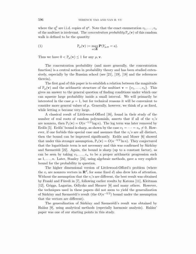
where the ηµi are i.i.d. copies of ηµ. Note that the exact enumeration v1, . . . , vnof the multiset is irrelevant. The concentration probability Pµ(v) of this randomwalk is defined to be the quantity
(1) Pµ(v) := maxa∈Z
P(Yµ,v = a).
Thus we have 0 < Pµ(v) ≤ 1 for any µ,v.
The concentration probability (and more generally, the concentrationfunction) is a central notion in probability theory and has been studied exten-sively, especially by the Russian school (see [21], [19], [18] and the referencestherein).
The first goal of this paper is to establish a relation between the magnitudeof Pµ(v) and the arithmetic structure of the multiset v = v1, . . . , vn. Thisgives an answer to the general question of finding conditions under which onecan squeeze large probability inside a small interval. We will primarily beinterested in the case µ = 1, but for technical reasons it will be convenient toconsider more general values of µ. Generally, however, we think of µ as fixed,while letting n become very large.
A classical result of Littlewood-Offord [16], found in their study of thenumber of real roots of random polynomials, asserts that if all of the vi’sare nonzero, then P1(v) = O(n−1/2 log n). The log term was later removed byErdos [5]. Erdos’ bound is sharp, as shown by the case v1 = · · · = vn 6= 0. How-ever, if one forbids this special case and assumes that the vi’s are all distinct,then the bound can be improved significantly. Erdos and Moser [6] showedthat under this stronger assumption, P1(v) = O(n−3/2 lnn). They conjecturedthat the logarithmic term is not necessary and this was confirmed by Sarkozyand Szemeredi [22]. Again, the bound is sharp (up to a constant factor), ascan be seen by taking v1, . . . , vn to be a proper arithmetic progression suchas 1, . . . , n. Later, Stanley [24], using algebraic methods, gave a very explicitbound for the probability in question.
The higher dimensional version of Littlewood-Offord’s problem (wherethe vi are nonzero vectors in Rd, for some fixed d) also drew lots of attention.Without the assumption that the vi’s are different, the best result was obtainedby Frankl and Furedi in [7], following earlier results by Katona [11], Kleitman[12], Griggs, Lagarias, Odlyzko and Shearer [8] and many others. However,the techniques used in these papers did not seem to yield the generalizationof Sarkozy and Szemeredi’s result (the O(n−3/2) bound under the assumptionthat the vectors are different).
The generalization of Sarkozy and Szemeredi’s result was obtained byHalasz [9], using analytical methods (especially harmonic analysis). Halasz’paper was one of our starting points in this study.
INVERSE LITTLEWOOD-OFFORD AND CONDITION NUMBER 597
In the above two examples, we see that in order to make Pµ(v) large, wehave to impose a very strong additive structure on v (in one case we set the vi’sto be the same, while in the other we set them to be elements of an arithmeticprogression). We are going to show that this is the only way to make Pµ(v)large. More precisely, we propose the following phenomenon:
If Pµ(v) is large, then v has a strong additive structure.
In the next section, we are going to present several theorems supportingthis phenomenon. Let us mention here that there is an analogous phenomenonin combinatorial number theory. In particular, a famous theorem of Freimanasserts that if A is a finite set of integers and A+A is small, then A is containedefficiently in a generalized arithmetic progression [28, Ch. 5]. However, theproofs of Freiman’s theorem and those in this paper are quite different.
As an application, we are going to use these inverse theorems to studyrandom matrices. Let Mµ
n be an n by n random matrix, whose entries arei.i.d. copies of ηµ. We are going to show that with very high probability,the condition number of Mµ
n is bounded from above by a polynomial in n
(see Theorem 3.3 below). This result has high potential of applications inthe theory of probability in Banach spaces, as well as in numerical analysisand theoretical computer science. A related result was recently established byRudelson [20], with better upper bounds on the condition number but worseprobabilities. We will discuss this application with more detail in Section 3.
To see the connection between this problem and inverse Littlewood-Offordtheory, observe that for any v = (v1, . . . , vn) (which we interpret as a columnvector), the entries of the product Mµ
nv are independent copies of Yµ,v. Thuswe expect that vT is unlikely to lie in the kernel of Mµ
n unless the concentrationprobability Pµ(v) is large. These ideas are already enough to control thesingularity probability of Mµ
n (see e.g. [10], [25], [26]). To obtain the morequantitative condition number estimates, we introduce a new discretizationtechnique that allows one to estimate the probability that a certain randomvariable is small by the probability that a certain discretized analogue of thatvariable is zero.
The rest of the paper is organized as follows. In Section 2 we state ourmain inverse theorems. In Section 3 we state our main results on conditionnumbers, as well as the key lemmas used to prove these results. In Section 4,we give some brief applications of the inverse theorems. In Section 7 we provethe result on condition numbers, assuming the inverse theorems and two otherkey ingredients: a discretization of generalized progressions and an extensionof the famous result of Kahn, Komlos and Szemeredi [10] on the probabilitythat a random Bernoulli matrix is singular. The inverse theorems is provenin Section 6, after some preliminaries in Section 5 in which we establish basicproperties of Pµ(v). The result about discretization of progressions are proven
598 TERENCE TAO AND VAN H. VU
in Section 8. Finally, in Section 9 we prove the extension of Kahn, Komlos andSzemeredi [10].
We conclude this section by setting out some basic notation. A set
P = c+m1a1 + · · ·+mdad|Mi ≤ mi ≤M ′i
is called a generalized arithmetic progression (GAP) of rank d. It is convenientto think of P as the image of an integer box
B := (m1, . . . ,md)|Mi ≤ mi ≤M ′i
in Zd under the linear map
Φ : (m1, . . . ,md) 7→ c+m1a1 + · · ·+mdad.
The numbers ai are the generators of P . In this paper, all GAPs have ra-tional generators. A GAP is proper if Φ is one to one on B. The product∏di=1(M ′i −Mi + 1) is the volume of P . If Mi = −M ′i and c = 0 (so P = −P )
then we say that P is symmetric.For a set A of reals and a positive integer k, we define the iterated sumset
kA := a1 + · · ·+ ak|ai ∈ A.
One should take care to distinguish the sumset kA from the dilate k ·A, definedfor any real k as
k ·A := ka|a ∈ A.
We always assume that n is sufficiently large. The asymptotic notationO(), o(), Ω(), Θ() is used under the assumption that n → ∞. Notation suchas Od(f) means that the hidden constant in O depends only on d.
2. Inverse Littlewood-Offord theorems
Let us start by presenting an example when Pµ(v) is large. This exampleis the motivation of our inverse theorems.
Example 2.1. Let P be a symmetric generalized arithmetic progression ofrank d and volume V ; we view d as being fixed independently of n, though V
can grow with n. Let v1, . . . , vn be (not necessarily different) elements of V .Then the random variable Yµ,v =
∑ni=1 ηivi takes values in the GAP nP which
has volume ndV . From the pigeonhole principle it follows that
Pµ(v) ≥ n−dV −1.
In fact, the central limit theorem suggests that Pµ(v) should typically be ofthe order of n−d/2V −1.
INVERSE LITTLEWOOD-OFFORD AND CONDITION NUMBER 599
This example shows that if the elements of v belong to a GAP with smallrank and small volume then Pµ(v) is large. One might hope that the inversealso holds, namely,
If Pµ(v) is large, then (most of ) the elements of v belong to a GAP withsmall rank and small volume.
In the rest of this section, we present three theorems, which support thisstatement in a quantitative way.
Definition 2.2 (Dissociativity). Given a multiset w = w1, . . . , wr ofreal numbers and a positive number k, we define the GAP Q(w, k) and thecube S(w) as follows:
Q(w, k) := m1w1 + · · ·+mrwr| − k ≤ mi ≤ k,S(w) := ε1w1 + · · ·+ εrwr|εi ∈ −1, 1.
We say that w is dissociated if S(w) does not contain zero. Furthermore, w isk-dissociated if there do not exist integers −k ≤ m1, . . . ,mr ≤ k, not all zero,such that m1w1 + · · ·+mrwr = 0.
Our first result is the following simple proposition:
Proposition 2.3 (Zeroth inverse theorem). Let v = v1, . . . , vn be suchthat P1(v) > 2−d−1 for some integer d ≥ 0. Then v contains a subset w ofsize d such that the cube S(w) contains v1, . . . , vn.
The next two theorems are more involved and also more useful. In thesetwo theorems and their corollaries, we assume that k and n are sufficientlylarge, whenever needed.
Theorem 2.4 (First inverse theorem). Let µ be a positive constant atmost 1 and let d be a positive integer. Then there is a constant C=C(µ, d)≥1such that the following holds. Let k ≥ 2 be an integer and let v = v1, . . . , vnbe a multiset such that
Pµ(v) ≥ C(µ, d)k−d.
Then there exists a k-dissociated multiset w = w1, . . . , wr such that
(1) r ≤ d− 1 and w1, . . . , wr are elements of v;
(2) The union⋃τ∈Z,1≤τ≤k
1τ · Q(w, k) contains all but k2 of the integers
v1, . . . , vn (counting multiplicity).
This theorem should be compared against the heuristics in Example 2.1(setting k equal to a small multiple of
√n). In particular, note that the GAP
Q(w, k) has very small volume, only O(kd−1).
600 TERENCE TAO AND VAN H. VU
The above theorem does not yet show that most of the elements of vbelong to a single GAP. Instead, it shows that they belong to the union of afew dilates of a GAP. One could remove the unwanted 1
τ factor by clearingdenominators, but this costs us an exponential factor such as k!, which is oftentoo large in applications. Fortunately, a more refined argument allows us toeliminate these denominators while losing only polynomial factors in k:
Theorem 2.5 (Second inverse theorem). Let µ be a positive constant atmost one, ε be an arbitrary positive constant and d be a positive integer. Thenthere are constants C = C(µ, ε, d) ≥ 1 and k0 = k0(µ, ε, d) ≥ 1 such that thefollowing holds. Let k ≥ k0 be an integer and let v = v1, . . . , vn be a multisetsuch that
Pµ(v) ≥ Ck−d.
Then there exists a GAP Q with the following properties:
(1) The rank of Q is at most d− 1;
(2) The volume of Q is at most k2(d2−1)+ε;
(3) Q contains all but at most εk2 log k elements of v (counting multiplicity);
(4) There exists a positive integer s at most kd+ε such that su ∈ v for eachgenerator u of Q.
Remark 2.6. A small number of exceptional elements cannot be avoided.For instance, one can add O(log k) completely arbitrary elements to v, anddecrease Pµ(v) by a factor of k−O(1) at worst.
For the applications in this paper, the following corollary of Theorem 2.5is convenient.
Corollary 2.7. For any positive constants A and α there is a positiveconstant A′ such that the following holds. Let µ be a positive constant atmost one and assume that v = v1, . . . , vn is a multiset of integers satisfyingPµ(v) ≥ n−A. Then there is a GAP Q of rank at most A′ and volume at mostnA′
which contains all but at most nα elements of v (counting multiplicity).Furthermore, there exists a positive integer s ≤ nA
′such that su ∈ v for each
generator u of Q.
Remark 2.8. The assumption Pµ(v) ≥ n−A in all statements can be re-placed by the following more technical, but somewhat weaker, assumption that∫ 1
0
∏i=1
|(1− µ) + µ cos 2πviξ| dξ ≥ n−A.
The right-hand side is an upper bound for Pµ(v), provided that µ is sufficientlysmall. Assuming that Pµ(v) ≥ n−A, what is actually used in the proofs is the
INVERSE LITTLEWOOD-OFFORD AND CONDITION NUMBER 601
consequence ∫ 1
0
∏i=1
|(1− µ) + µ cos 2πviξ|dξ ≥ n−A.
(See §5 for more details.) This weaker assumption is useful in applications (see[27]).
The vector versions of all three theorems hold (when the vi’s are vectorsin Rr, for any positive integer r), thanks to Freiman’s isomorphism principle(see, e.g., [28, Ch. 5]). This principle allows us to project the problem from Rr
onto Z. The value of r is irrelevant and does not appear in any quantitativebound. In fact, one can even replace Rr by any torsion free additive group.
In an earlier paper [26] we introduced another type of inverse Littlewood-Offord theorem. This result showed that if Pµ(v) was comparable to P1(v),then v could be efficiently contained inside a GAP of bounded rank (see [26,Th. 5.2] for details).
We shall prove these inverse theorems in Section 6, after some combina-torial and Fourier-analytic preliminaries in Section 5. For now, we take theseresults for granted and turn to an application of these inverse theorems torandom matrices.
3. The condition number of random matrices
If M is an n× n matrix, we use
σ1(M) := supx∈Rn
,‖x‖=1
‖Mx‖
to denote the largest singular value of M . Tthis parameter is also often calledthe operator norm of M . Here ‖x‖ denotes the Euclidean magnitude of avector x ∈ Rn. If M is invertible, the condition number c(M) is defined as
c(M) := σ1(M)σ1(M−1).
We adopt the convention that c(M) is infinite if M is not invertible.The condition number plays a crucial role in applied linear algebra and
computer science. In particular, the complexity of any algorithm which re-quires solving a system of linear equations usually involves the condition num-ber of a matrix; see [1], [23]. Another area of mathematics where this parameteris important is the theory of probability in Banach spaces (e.g. see [15], [20]).
The condition number of a random matrix is a well-studied object (see[3] and the references therein). In the case when the entries of M are i.i.d.Gaussian random variables (with mean zero and variance one), Edelman [3],answering a question of Smale [23] showed
602 TERENCE TAO AND VAN H. VU
Theorem 3.1. Let Nn be an n × n random matrix, whose entries arei.i.d. Gaussian random variables (with mean zero and variance one). ThenE(ln c(Nn)) = lnn+ c+ o(1), where c > 0 is an explicit constant.
In application, it is usually useful to have a tail estimate. It was shownby Edelman and Sutton [4] that
Theorem 3.2. Let Nn be a n by n random matrix, whose entries are i.i.d.Gaussian random variables (with mean zero and variance one). Then for anyconstant A > 0,
P(c(Nn) ≥ nA+1) = OA(n−A).
On the other hand, for the other basic case when the entries are i.i.d.Bernoulli random variables (copies of η1), the situation is far from being settled.Even to prove that the condition number is finite with high probability is anontrivial task (see [13]). The techniques used to study Gaussian matrices relyheavily on the explicit joint distribution of the eigenvalues. This distributionis not available for discrete models.
Using our inverse theorems, we can prove the following result, which iscomparable to Theorem 3.2, and is another main result of this paper. Let Mµ
n
be the n by n random matrix whose entries are i.i.d. copies of ηµ. In particular,the Bernoulli matrix mentioned above is the case when µ = 1.
Theorem 3.3. For any positive constant A, there is a positive constantB such that the following holds. For any positive constant µ at most one andany sufficiently large n
P(c(Mµn ) ≥ nB) ≤ n−A.
Given an invertible matrix M of order n, we set σn(M) to be the smallestsingular value of M :
σn(M) := minx∈Rn
,‖x‖=1‖Mx‖.
Thenc(M) = σ1(M)/σn(M).
It is well known that there is a constant Cµ such that the largest singularvalue of Mµ
n is at most Cµn1/2 with exponential probability 1− exp(−Ωµ(n))(see, e.g. [14]). Thus, Theorem 3.3 reduces to the following lower tail estimatefor the smallest singular value of σn(M):
Theorem 3.4. For any positive constant A, there is a positive constantB such that the following holds. For any positive constant µ at most one andany sufficiently large n
P(σn(Mµn ) ≤ n−B) ≤ n−A.
INVERSE LITTLEWOOD-OFFORD AND CONDITION NUMBER 603
Shortly prior to this paper, Rudelson [20] proved the following result.
Theorem 3.5. Let 0 < µ ≤ 1. There are positive constants c1(µ), c2(µ)such that the following holds. For any ε ≥ c1(µ)n−1/2,
P(σn(Mµn ) ≤ c2(µ)εn−3/2) ≤ ε.
In fact, Rudelson’s result holds for a larger class of matrices. The descrip-tion of this class is, however, somewhat technical. We refer the reader to [20]for details.
It is useful to compare Theorems 3.4 and 3.5. Theorem 3.5 gives anexplicit dependence between the bound on σn and the probability, while thedependence between A and B in Theorem 3.4 is implicit. Actually our proofdoes provide an explicit value for B, but it is rather large and we make noattempt to optimize it. On the other hand, Theorem 3.5 does not yield aprobability better than n−1/2. In many applications (especially those involvingthe union bound), it is important to have a probability bound of order n−A
with arbitrarily given A.The proof of Theorem 3.4 relies on Corollary 2.7 and two other ingredients,
which are of independent interest. In the rest of this section, we discuss theseingredients. These ingredients will then be combined in Section 7 to proveTheorem 3.4.
3.1. Discretization of GAPs. Let P be a GAP of integers of rank d andvolume V . We show that given any specified scale parameter R0, one can“discretize” P near the scale R0. More precisely, one can cover P by the sumof a coarse progression and a small progression, where the diameter of the smallprogression is much smaller (by an arbitrarily specified factor of S) than thespacing of the coarse progression, and that both of these quantities are closeto R0 (up to a bounded power of SV ).
Theorem 3.6 (Discretization). Let P ⊂ Z be a symmetric GAP of rankd and volume V . Let R0, S be positive integers. Then there exists a scale R ≥ 1and two GAPs Psmall, Psparse of rational numbers with the following properties.
• (Scale) R = (SV )Od(1)R0.
• (Smallness) Psmall has rank at most d, volume at most V , and takesvalues in [−R/S,R/S].
• (Sparseness) Psparse has rank at most d, volume at most V , and any twodistinct elements of SPsparse are separated by at least RS.
• (Covering) P ⊆ Psmall + Psparse.
604 TERENCE TAO AND VAN H. VU
This theorem is elementary but is somewhat involved. The detailed proofwill appear in Section 8. Here, we give an informal explanation, appealingto the analogy between the combinatorics of progressions and linear algebra.Recall that a GAP of rank d is the image Φ(B) of a d-dimensional box undera linear map Φ. This can be viewed as a discretized, localized analogue of theobject Φ(V ), where Φ is a linear map from a d-dimensional vector space Vto some other vector space. The analogue of a “small” progression would bean object Φ(V ) in which Φ vanished. The analogue of a “sparse” progressionwould be an object Φ(V ) in which the map Φ was injective. Theorem 3.6 isthen a discretized, localized analogue of the obvious linear algebra fact thatgiven any object of the form Φ(V ), one can split V = Vsmall +Vsparse for whichΦ(Vsmall) is small and Φ(Vsparse) is sparse. Indeed one simply sets Vsmall tobe the kernel of Φ, and Vsparse to be any complementary subspace to Vsmall
in V . The proof of Theorem 3.6 follows these broad ideas, with Psmall be-ing essentially a “kernel” of the progression P , and Psparse being a kind of“complementary progression” to this kernel.
To oversimplify, we shall exploit this discretization result (as well as theinverse Littlewood-Offord theorems) to control the event that the singular valueis small, by the event that the singular value (of a slightly modified randommatrix) is zero. The control of this latter quantity is the other ingredient ofthe proof, to which we now turn.
3.2. Singularity of random matrices. A famous result of Kahn, Komlosand Szemeredi [10] asserts that the probability that M1
n is singular (or equiv-alently, that σn(M1
n) = 0) is exponentially small:
Theorem 3.7. There is a positive constant ε such that
P(σn(M1n) = 0) ≤ (1− ε)n.
In [10] it was shown that one can take ε = .001. Improvements on ε areobtained recently in [25], [26]. The value of ε does not play a critical role inthis paper.
To prove Theorem 3.3, we need the following generalization of Theo-rem 3.7. Note that the row vectors of M1
n are i.i.d. copies of X1, whereX1 = (η1
1, . . . , η1n) and η1
i are i.i.d. copies of η1. By changing 1 to µ, we candefine Xµ in the obvious manner. Now let Y be a set of l vectors y1, . . . , yl inRn and Mµ,Y
n be the random matrix whose rows are Xµ1 , . . . , X
µn−l, y1, . . . , yl,
where Xµi are i.i.d. copies of Xµ.
Theorem 3.8. Let 0 < µ ≤ 1, and let l be a nonnegative integer. Thenthere is a positive constant ε= ε(µ, l) such that the following holds. For anyset Y of l independent vectors from Rn,
P(σn(Mµ,Yn ) = 0) ≤ (1− ε)n.
INVERSE LITTLEWOOD-OFFORD AND CONDITION NUMBER 605
Corollary 3.9. Let 0 < µ ≤ 1. Then there is a positive constant ε =ε(µ) such that the following holds. For any vector y ∈ Rn, the probability thatthere are w1, . . . , wn−1, not all zeros, such that
y = Xµ1w1 + . . . Xµ
n−1wn−1
is at most (1− ε)n.
We will prove Theorem 3.10 in Section 9 by using the machinery from [25].
4. Some quick applications of the inverse theorems
The inverse theorems provide effective bounds for counting the numberof “exceptional” collections v of numbers with high concentration probability;see [26] for a demonstration of how such bounds can be used in applications. Inthis section, we present two such bounds that can be obtained from the inversetheorems developed here. In the first example, let ε be a positive constant andM be a large integer, and consider the following question:
How many sets v of n integers with absolute values at most M are theresuch that P1(v) ≥ ε?
By Erdos’ result, all but at most O(ε−2) of the elements of v are nonzero.Thus we have the upper bound
(nε−2
)(2M+1)O(ε−2) for the number in question.
Using Proposition 2.3, we can obtain a better bound as follows. There are onlyMO(ln ε−1) ways to choose the generators of the cube. After the cube is fixed,we need to choose O(ε−2) nonzero elements inside it. As the cube has volumeO(ε−1), the number of ways to do this is (1
ε )O(ε−2). Thus, we end up with a
bound
MO(ln ε−1)
(1ε
)O(ε−2)
which is better than the previous bound if M is considerably larger than ε−1.For the second application, we return to the question of bounding the sin-
gularity probability P(σn(M1n) = 0) studied in Theorem 3.7. This probability
is conjectured to equal (1/2 + o(1))n, but this remains open (see [26] for thelatest results and some further discussion). The event that M1
n is singular isthe same as the event that there exists some nonzero vector v ∈ Rn such thatM1nv = 0. For simplicity, we use the notation Mn instead of M1
n in the rest ofthis section. It turns out that one can obtain the optimal bound (1/2 + o(1))n
if one restricts v to some special set of vectors.Let Ω1 be the set of vectors in Rn with at least 3n/ log2 n coordinates.
Komlos proved the following:
Theorem 4.1. The probability that Mnv = 0 for some nonzero v ∈ Ω1 is(1/2 + o(1))n.
606 TERENCE TAO AND VAN H. VU
A proof of this theorem can be found in Bollobas’ book [2].We are going to consider another restricted class. Let C be an arbitrary
positive constant and let Ω2 be the set of integer vectors in Rn where thecoordinates have absolute values at most nC . Using Theorem 2.4, we canprove
Theorem 4.2. The probability that Mnv = 0 for some nonzero v ∈ Ω2 is(1/2 + o(1))n.
Proof. The lower bound is trivial so we focus on the upper bound. Foreach nonzero vector v, let p(v) be the probability that X · v = 0, where X isa random Bernoulli vector. From independence we have P(Mnv = 0) = p(v)n.Since a hyperplane can contain at most 2n−1 vectors from −1,+1n, p(v) isat most 1/2. For j = 1, 2, . . . , let Sj be the number of nonzero vectors v in Ω2
such that 2−j−1 < p(v) ≤ 2−j . Then the probability that Mnv = 0 for somenonzero v ∈ Ω2 is at most
n∑j=1
(2−j)nSj .
Let us now restrict the range of j. Note that if p(v) ≥ n−1/3, then by Erdos’sresult (mentioned in the introduction) most of the coordinates of v are zero. Inthis case, by Theorem 4.1 the contribution from these v is at most (1/2+o(1))n.Next, since the number of vectors in Ω2 is at most (2nC + 1)n ≤ n(C+1)n, wecan ignore those j where 2−j ≤ n−C−2. Now it suffices to show that∑
n−C−2≤2−j≤n−1/3
(2−j)nSj = o((1/2)n).
For any relevant j, we can find an integer d = O(1) and a positive numberε = Ω(1) such that
n−(d−1/3)ε ≤ 2−j < n−(d−2/3)ε.
Set k := nε. Thus 2−j k−d and we can use Theorem 2.4 to esti-mate Sj . Indeed, by invoking this theorem, we see that there are at most(nk2
)(2nC + 1)k
2= nO(k2
) = no(n) ways to choose the positions and values ofexceptional coordinates of v. Furthermore, there are only (2nC+1)d−1 = nO(1)
ways to fix the generalized progression P := Q(w, k).Note that the elements of P are polynomially bounded in n. Such integers
have only no(1 divisors. Thus, if P is fixed any (nonexceptional) coordinateof v has at most |P |no(1) possible values. This means that once P is fixed,the number of ways to set the nonexceptional coordinates of v is at most(no(1)|P |)n = (2k + 1)(d−1+o(1))n. Putting these together,
Sj ≤ nO(k2)k(d−1+o(1))n.
INVERSE LITTLEWOOD-OFFORD AND CONDITION NUMBER 607
As k = nε and 2−j ≤ n−(d−2/3)ε, it follows that
2−jnSj ≤ no(n)n−εn/3 = o
(1
log n
)2−n.
Since there are only O(log n) relevant j, we can conclude the proof by summingthe bound over j.
5. Properties of Pµ(v)
In order to prove the inverse Littlewood-Offord theorems in Section 2,we shall first need to develop some useful tools for estimating the quantityPµ(v). Note that the tools here are only used for the proof of the inverseLittlewood-Offord theorems in Section 6 and are not required elsewhere in thepaper.
It is convenient to think of v as a word, obtained by concatenating thenumbers vi:
v = v1v2 . . . vn.
This allows us to perform several operations such as concatenating, truncatingand repeating. For instance, if v = v1 . . . vn and w = w1 . . . wm, then
Pµ(vw) = maxa∈Z
( n∑i=1
ηµi vi +m∑j=1
ηµn+jwj = a)
where ηµk , 1 ≤ k ≤ n + m are i.i.d. copies of ηµ. Furthermore, we use vk todenote the concatenation of k copies of v.
It turns out that there is a nice calculus concerning the expressions Pµ(v),especially when µ is small. The core properties are summarized in the nextlemma.
Lemma 5.1. The following properties hold.
• Pµ(v) is invariant under permutations of v.
• For any words v,w
(2) Pµ(v)Pµ(w) ≤ Pµ(vw) ≤ Pµ(v).• For any 0 < µ ≤ 1, any 0 < µ′ ≤ µ/4, and any word v,
(3) Pµ(v) ≤ Pµ′(v).• For any number 0 < µ ≤ 1/2 and any word v,
(4) Pµ(v) ≤ Pµ/k(vk).• For any number 0 < µ ≤ 1/2 and any words v,w1, . . . ,wm,
(5) Pµ(vw1 . . .wm) ≤( m∏j=1
Pµ(vwmj ))1/m
.
608 TERENCE TAO AND VAN H. VU
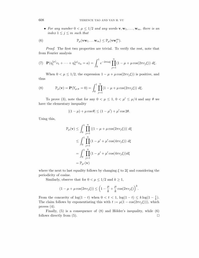
• For any number 0 < µ ≤ 1/2 and any words v,w1, . . . ,wm, there is anindex 1 ≤ j ≤ m such that
(6) Pµ(vw1 . . .wm) ≤ Pµ(vwmj ).
Proof. The first two properties are trivial. To verify the rest, note thatfrom Fourier analysis
(7) P(η(µ)1 v1 + · · ·+ η(µ)
n vn = a) =∫ 1
0e−2πiaξ
n∏j=1
(1− µ+ µ cos(2πvjξ)) dξ.
When 0 < µ ≤ 1/2, the expression 1 − µ + µ cos(2πvjξ)) is positive, andthus
(8) Pµ(v) = P(Yµ,v = 0) =∫ 1
0
n∏j=1
(1− µ+ µ cos(2πvjξ)) dξ.
To prove (3), note that for any 0 < µ ≤ 1, 0 < µ′ ≤ µ/4 and any θ wehave the elementary inequality
|(1− µ) + µ cos θ| ≤ (1− µ′) + µ′ cos 2θ.
Using this,
Pµ(v) ≤∫ 1
0
n∏j=1
|(1− µ+ µ cos(2πvjξ))| dξ
≤∫ 1
0
n∏j=1
(1− µ′ + µ′ cos(4πvjξ)) dξ
=∫ 1
0
n∏j=1
(1− µ′ + µ′ cos(4πvjξ))dξ
= Pµ′(v)
where the next to last equality follows by changing ξ to 2ξ and considering theperiodicity of cosine.
Similarly, observe that for 0 < µ ≤ 1/2 and k ≥ 1,
(1− µ+ µ cos(2πvjξ)) ≤(
1− µ
k+µ
kcos(2πvjξ)
)k.
From the concavity of log(1 − t) when 0 < t < 1, log(1 − t) ≤ k log(1 − tk ).
The claim follows by exponentiating this with t := µ(1 − cos(2πvjξ))), whichproves (4).
Finally, (5) is a consequence of (8) and Holder’s inequality, while (6)follows directly from (5).
INVERSE LITTLEWOOD-OFFORD AND CONDITION NUMBER 609
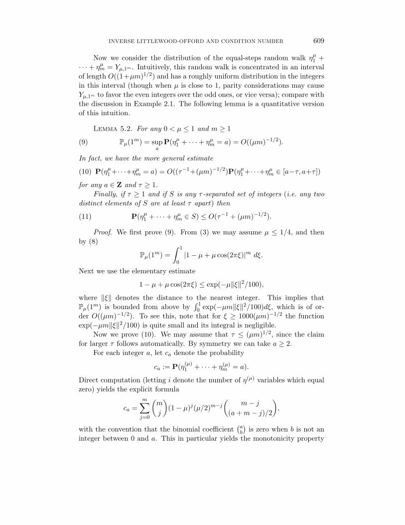
Now we consider the distribution of the equal-steps random walk ηµ1 +· · ·+ ηµm = Yµ,1m . Intuitively, this random walk is concentrated in an intervalof length O((1+µm)1/2) and has a roughly uniform distribution in the integersin this interval (though when µ is close to 1, parity considerations may causeYµ,1m to favor the even integers over the odd ones, or vice versa); compare withthe discussion in Example 2.1. The following lemma is a quantitative versionof this intuition.
Lemma 5.2. For any 0 < µ ≤ 1 and m ≥ 1
(9) Pµ(1m) = supa
P(ηµ1 + · · ·+ ηµm = a) = O((µm)−1/2).
In fact, we have the more general estimate
(10) P(ηµ1 +· · ·+ηµm = a) = O((τ−1+(µm)−1/2)P(ηµ1 +· · ·+ηµm ∈ [a−τ, a+τ ])
for any a ∈ Z and τ ≥ 1.Finally, if τ ≥ 1 and if S is any τ -separated set of integers (i.e. any two
distinct elements of S are at least τ apart) then
(11) P(ηµ1 + · · ·+ ηµm ∈ S) ≤ O(τ−1 + (µm)−1/2).
Proof. We first prove (9). From (3) we may assume µ ≤ 1/4, and thenby (8)
Pµ(1m) =∫ 1
0|1− µ+ µ cos(2πξ)|m dξ.
Next we use the elementary estimate
1− µ+ µ cos(2πξ) ≤ exp(−µ‖ξ‖2/100),
where ‖ξ‖ denotes the distance to the nearest integer. This implies thatPµ(1m) is bounded from above by
∫ 10 exp(−µm‖ξ‖2/100)dξ, which is of or-
der O((µm)−1/2). To see this, note that for ξ ≥ 1000(µm)−1/2 the functionexp(−µm‖ξ‖2/100) is quite small and its integral is negligible.
Now we prove (10). We may assume that τ ≤ (µm)1/2, since the claimfor larger τ follows automatically. By symmetry we can take a ≥ 2.
For each integer a, let ca denote the probability
ca := P(η(µ)1 + · · ·+ η(µ)
m = a).
Direct computation (letting i denote the number of η(µ) variables which equalzero) yields the explicit formula
ca =m∑j=0
(m
j
)(1− µ)j(µ/2)m−j
(m− j
(a+m− j)/2
),
with the convention that the binomial coefficient(ab
)is zero when b is not an
integer between 0 and a. This in particular yields the monotonicity property
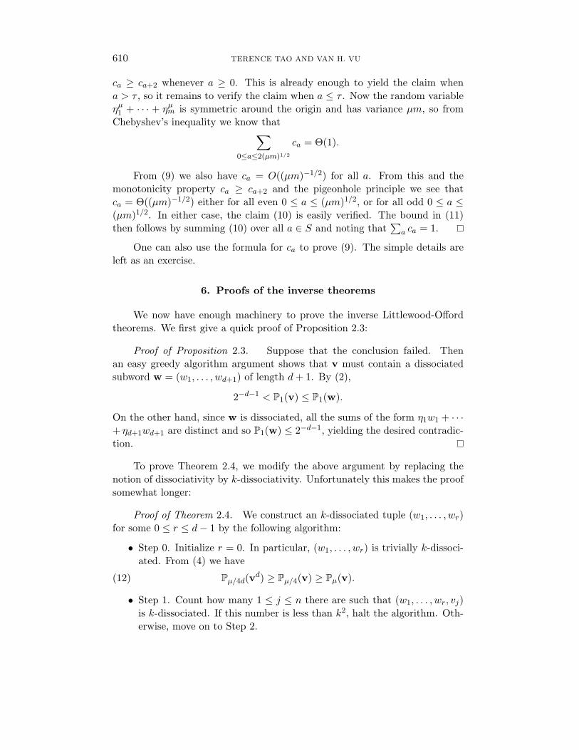
610 TERENCE TAO AND VAN H. VU
ca ≥ ca+2 whenever a ≥ 0. This is already enough to yield the claim whena > τ , so it remains to verify the claim when a ≤ τ . Now the random variableηµ1 + · · · + ηµm is symmetric around the origin and has variance µm, so fromChebyshev’s inequality we know that∑
0≤a≤2(µm)1/2
ca = Θ(1).
From (9) we also have ca = O((µm)−1/2) for all a. From this and themonotonicity property ca ≥ ca+2 and the pigeonhole principle we see thatca = Θ((µm)−1/2) either for all even 0 ≤ a ≤ (µm)1/2, or for all odd 0 ≤ a ≤(µm)1/2. In either case, the claim (10) is easily verified. The bound in (11)then follows by summing (10) over all a ∈ S and noting that
∑a ca = 1.
One can also use the formula for ca to prove (9). The simple details areleft as an exercise.
6. Proofs of the inverse theorems
We now have enough machinery to prove the inverse Littlewood-Offordtheorems. We first give a quick proof of Proposition 2.3:
Proof of Proposition 2.3. Suppose that the conclusion failed. Thenan easy greedy algorithm argument shows that v must contain a dissociatedsubword w = (w1, . . . , wd+1) of length d+ 1. By (2),
2−d−1 < P1(v) ≤ P1(w).
On the other hand, since w is dissociated, all the sums of the form η1w1 + · · ·+ ηd+1wd+1 are distinct and so P1(w) ≤ 2−d−1, yielding the desired contradic-tion.
To prove Theorem 2.4, we modify the above argument by replacing thenotion of dissociativity by k-dissociativity. Unfortunately this makes the proofsomewhat longer:
Proof of Theorem 2.4. We construct an k-dissociated tuple (w1, . . . , wr)for some 0 ≤ r ≤ d− 1 by the following algorithm:
• Step 0. Initialize r = 0. In particular, (w1, . . . , wr) is trivially k-dissoci-ated. From (4) we have
(12) Pµ/4d(vd) ≥ Pµ/4(v) ≥ Pµ(v).
• Step 1. Count how many 1 ≤ j ≤ n there are such that (w1, . . . , wr, vj)is k-dissociated. If this number is less than k2, halt the algorithm. Oth-erwise, move on to Step 2.
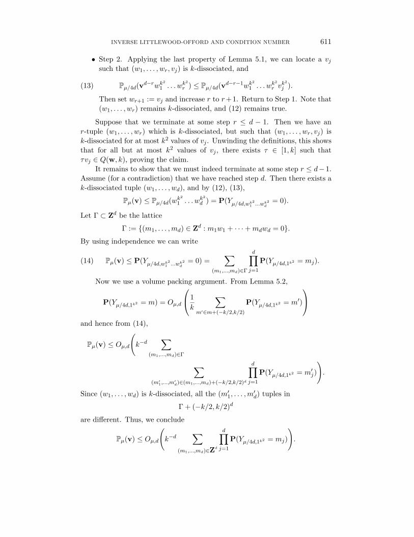
INVERSE LITTLEWOOD-OFFORD AND CONDITION NUMBER 611
• Step 2. Applying the last property of Lemma 5.1, we can locate a vjsuch that (w1, . . . , wr, vj) is k-dissociated, and
(13) Pµ/4d(vd−rwk2
1 . . . wk2
r ) ≤ Pµ/4d(vd−r−1wk2
1 . . . wk2
r vk2
j ).
Then set wr+1 := vj and increase r to r+1. Return to Step 1. Note that(w1, . . . , wr) remains k-dissociated, and (12) remains true.
Suppose that we terminate at some step r ≤ d − 1. Then we have anr-tuple (w1, . . . , wr) which is k-dissociated, but such that (w1, . . . , wr, vj) isk-dissociated for at most k2 values of vj . Unwinding the definitions, this showsthat for all but at most k2 values of vj , there exists τ ∈ [1, k] such thatτvj ∈ Q(w, k), proving the claim.
It remains to show that we must indeed terminate at some step r ≤ d− 1.Assume (for a contradiction) that we have reached step d. Then there exists ak-dissociated tuple (w1, . . . , wd), and by (12), (13),
Pµ(v) ≤ Pµ/4d(wk2
1 . . . wk2
d ) = P(Yµ/4d,wk21 ...wk2d
= 0).
Let Γ ⊂ Zd be the lattice
Γ := (m1, . . . ,md) ∈ Zd : m1w1 + · · ·+mdwd = 0.
By using independence we can write
(14) Pµ(v) ≤ P(Yµ/4d,wk21 ...wk2d
= 0) =∑
(m1,...,md)∈Γ
d∏j=1
P(Yµ/4d,1k2 = mj).
Now we use a volume packing argument. From Lemma 5.2,
P(Yµ/4d,1k2 = m) = Oµ,d
1k
∑m′∈m+(−k/2,k/2)
P(Yµ/4d,1k2 = m′)
and hence from (14),
Pµ(v) ≤ Oµ,d
(k−d
∑(m1,...,md)∈Γ ∑(m′1,...,m
′d)∈(m1,...,md)+(−k/2,k/2)d
d∏j=1
P(Yµ/4d,1k2 = m′j)
).
Since (w1, . . . , wd) is k-dissociated, all the (m′1, . . . ,m′d) tuples in
Γ + (−k/2, k/2)d
are different. Thus, we conclude
Pµ(v) ≤ Oµ,d
(k−d
∑(m1,...,md)∈Zd
d∏j=1
P(Yµ/4d,1k2 = mj)
).
612 TERENCE TAO AND VAN H. VU
But from the union bound
∑(m1,...,md)∈Zd
d∏j=1
P(Yµ/4d,1k2 = mj) = 1,
and soPµ(v) ≤ Oµ,d(k−d).
To complete the proof, set the constant C = C(µ, d) in the theorem to belarger than the hidden constant in Oµ,d(k−d).
Remark 6.1. One can also use the Chernoff bound and obtain a shorterproof (avoiding the volume packing argument) but with an extra logarithmicloss in the estimates.
Finally we perform some additional arguments to eliminate the 1τ dilations
in Theorem 2.4 and obtain our final inverse Littlewood-Offord theorem. Thekey will be the following lemma.
Given a set S and a number v, the torsion of v with respect to S is thesmallest positive integer τ such that τv ∈ S. If such τ does not exists, we saythat v has infinite torsion with respect to S.
The key new ingredient will be the following lemma, which asserts thatadding a high torsion element to a random walk reduces the concentrationprobability significantly.
Lemma 6.2 (Torsion implies dispersion). Let 0 < µ ≤ 1 and consider aGAP Q :=
∑di=1 xiWi|−Li ≤ xi ≤ Li. Assume that Wd+1 has finite torsion
τ with respect to 2Q. Then there is a constant Cµ depending only on µ suchthat
Pµ(WL11 . . .WLd
d W τ2
d+1) ≤ Cµτ−1Pµ(WL11 . . .WLd
d ).
Proof. Let a be an integer such that
Pµ(WL11 . . .WLd
d W τ2
d+1) = P
(d∑i=1
Wi
Li∑j=1
ηµj,i +Wd+1
τ2∑j=1
ηµj,d+1 = a
),
where the ηµj,i are i.i.d. copies of ηµ. It suffices to show that
P
d∑i=1
Wi
Li∑j=1
ηµj,i +Wd+1
τ2∑j=1
ηµj,d+1 = a
= Oµ(τ−1)Pµ(WL11 . . .WLd
d ).
Let S be the set of all m ∈ [−τ2, τ2] such that Q + mWd+1 contains a.Observe that in order for
∑di=1Wi
∑Lij=1 η
µj,i+Wd+1
∑τ2
j=1 ηµj,d+1 to equal a, the
INVERSE LITTLEWOOD-OFFORD AND CONDITION NUMBER 613
quantity∑k
j=1 ηµj,d+1 must lie in S. By the definition of Pµ(WL1
1 . . .WLdd ) and
Bayes identity, we conclude
P
(d∑i=1
Wi
Li∑j=1
ηµj,i +Wd+1
τ2∑j=1
ηµj,d+1 = a
)
≤ Pµ(WL11 . . .WLd
d )P
(τ2∑j=1
ηµj,d+1 ∈ S
).
Consider two elements x, y ∈ S. By the definition of S, (x−y)v ∈ Q−Q =2Q. From the definition of τ , |x− y| is either zero or at least τ . This impliesthat S is τ -separated and the claim now follows from Lemma 5.2.
The following technical lemma is also needed.
Lemma 6.3. Consider a GAP Q(w, L). Assume that v is an element with(finite) torsion τ with respect to Q(w, L). Then
Q(w, L) +Q(v, L′) ⊂ 1τ·Q(w, L(L′ + τ)).
Proof. Assume w = w1 . . . wr. We can write v as 1τ
∑ri=1 aiwi, where
|ai| ≤ L. An element y in Q(w, L) +Q(v, L′) can be written as
y =r∑i=1
xiwi + xv
where |xi| ≤ L and |x| ≤ L′. Substituting v,
y =r∑i=1
xiwi + x1τ
r∑i=1
aiwi =1τ
r∑i=1
wi(τxi + xai),
where |τxi + xai| ≤ τL+ L′L. This concludes the proof.
Proof of Theorem 2.5. We begin by running the algorithm in the proofof Theorem 2.4 to locate a word w of length at most d − 1 such that the set⋃
1≤τ≤k1τ ·Q(w, k) covers all but at most k2 elements of v. Set v[0] to be the
word formed by removing the (at most k2) exceptional elements from v whichdo not lie in
⋃1≤τ≤k
1τ ·Q(w, k).
By increasing the constant k0 in the assumption of the theorem, we canassume, in all arguments below, that k is sufficiently large, whenever needed.
By (2) and (3)(15)
Pµ/4d(v[0]wk2) ≥ Pµ/4d(vwk2
) ≥ Pµ/4d(v)Pµ/4d(vwk2) ≥ k−dPµ/4d(vwk2
).
In the following, assume that there is at least one nonzero entry in w;otherwise the claim is trivial.
614 TERENCE TAO AND VAN H. VU
Now we perform an additional algorithm. Let K = K(µ, d, ε) > 2 be alarge constant to be chosen later.
• Step 0. Initialize i = 0 and set Q0 := Q(w, k2) and v[0] as above.
• Step 1. Count how many v ∈ v[i−1] having torsion at least K with re-spect to 2Qi−1. (We need to have the factor 2 here in order to applyLemma 6.2.) If this number is less than k2, halt the algorithm. Other-wise, move on to Step 2.
• Step 2. Locate a multiset S of k2 elements of v[i−1] with torsion at leastK with respect to 2Qi−1. Applying (6), we can find an element v ∈ Ssuch that
Pµ/4d(v[i−1]wk2W
τ21
1 . . .Wτ2i−1
i−1 ) ≤ Pµ/4d(v[i]wk2W
τ21
1 . . .Wτ2i−1
i−1 vk2
)
where v[i] is obtained from v[i−1] by deleting S.Let τi be the torsion of v with respect to 2Qi−1. Since every element ofv[0] has torsion at most k with respect to Q0, K ≤ τi ≤ k. We then setWi := v, Qi := Qi−1 +Q(Wi, τ
2i ), increase i to i+1 and return to Step 1.
Consider a stage i of the algorithm. From construction and inductionand (15), we have a word W1 . . .Wi with
Pµ/4d(v[i]wk2W
τ21
1 . . .Wτ2i
i ) ≥ P(v[0]wk2) ≥ k−dP(wk2
).
On the other hand, by applying Lemma 6.2 iteratively,
Pµ/4d(wk2W
τ21
1 . . .Wτ2i
i ) ≤ Pµ/4d(wk2)
i∏j=1
(Cµτ−1j ).
It follows that∏ij=1(Cµτ−1
j ) ≥ k−d, or equivalently∏ij=1(C−1
µ τj) ≤ kd. Recallthat τj ≥ K. Thus by setting K sufficiently large (compared to Cµ, d and 1/ε),we can guarantee that
(16)i∏
j=1
τj ≤ kd+ε/2d
where ε is the constant in the assumption of the theorem. It also follows thatthe algorithm must terminate at some stage D ≤ logK kd+ε/2d ≤ (d+1) logK k.
Now look at the final set QD. Applying Lemma 6.3 iteratively,
QD ⊂
(D∏j=1
1τj
)·Q(w, LD)
where L0 := k2 and
(17) Li := Li−1(τi + τ2i ) ≤ (1 + 1/K)Li−1τ
2i .
We now show that the GAP Q := 1K! ·(2K!)Q(w, LD) = 1
K! ·Q(w, 2K!LD)satisfies the claims of the theorem.
INVERSE LITTLEWOOD-OFFORD AND CONDITION NUMBER 615
• (Rank) We have rank(Q) = rank(Q(w, LD)) = rank(Q0) = r ≤ d − 1, asshown in the proof of the previous theorem.
• (Volume) We have Vol(Q) = (2K!)rVol(Q(w, LD)) = O(Vol(Q(w, LD))).On the other hand, by (16) and (17)
Vol(Q(w, LD)) = (2LD + 1)r ≤ (3LD)r =O
((k2
D∏j=1
(1 + 1/K)τ2j
)r)
=O
((k2+2(d+ε/2d)(1 +K)D
)r).
By definition, D ≤ logK kd+ε/2d < log k, given that K is sufficiently largecompared to d. Thus (1 + 1/K)D ≤ exp(D/K) ≤ k1/K which impliesthat
Vol(Q(w, LD)) = O(kr(2+2(d+ε/2d)+1/K)) = o(k2(d2−1)+ε)
provided that r ≤ d − 1 and K is sufficiently large compared to d and1/ε. (The asymptotic notation here is used under the assumption thatk →∞.)
• (Number of exceptional elements) At each stage in the second algorithm,we discard a set of k2 elements; thus all but Dk2 ≤ (d + 1)k2 logK k)elements of v[0] have torsion at most K with respect to 2QD. As QD ⊂Q(w, LD) and v\v[0] ≤ k2, it follows that all but at most
(d+ 1)k2 logK k + k2
elements of v have torsion at most K with respect to
2Q(w, LD) = Q(w, 2LD).
By setting K sufficiently large compared to d and 1/ε, we can guaranteethat
(d+ 1)k2 logK k + k2 ≤ εk2 log k.
To conclude, note that any element with torsion at most K with respectto Q(w, 2LD) belongs to Q := 1
K! · Q(w, 2K!LD). Thus, Q contains allbut at most εk2 log k elements of v.
• (Generators) The generators of 1K! · Q(w, 2K!LD) are 1
K!QDj=1 τj
wi, 1 ≤
i ≤ r. Since wi ∈ v and∏Dj=1 τj ≤ kd+ε/2d = o(kd+ε), the claim about
generators follows.
The proof is complete.
616 TERENCE TAO AND VAN H. VU
7. The smallest singular value
In this section, we prove Theorem 3.4, modulo two key results, Theo-rem 3.6 and Corollary 3.9, which will be proved in later sections.
Let B10 be a large number (depending on A) to be chosen later. Supposethat σn(Mµ
n ) < n−B. This means that there exists a unit vector v such that
‖Mµn v‖ < n−B.
By rounding each coordinate v to the nearest multiple of n−B−2, we canfind a vector v ∈ n−B−2 · Zn of magnitude 0.9 ≤ ‖v‖ ≤ 1.1 such that
‖Mµn v‖ ≤ 2n−B.
Thus, writing w := nB+2v, we can find an integer vector w ∈ Zn of magnitude0.9nB+2 ≤ ‖w‖ ≤ 1.1nB+2 such that
‖Mµnw‖ ≤ 2n2.
Let Ω be the set of integer vectors w ∈ Zn of magnitude 0.9nB+2 ≤ ‖w‖ ≤1.1nB+2. It suffices to show the probability bound
P(there is some w ∈ Ω such that ‖Mµnw‖ ≤ 2n2) = OA,µ(n−A).
We now partition the elements w = (w1, . . . , wn) of Ω into three sets:
• We say that w is rich if
Pµ(w1 . . . wn) ≥ n−A−10
and poor otherwise. Let Ω1 be the set of poor w’s.
• A rich w is singular w if fewer than n0.2 of its coordinates have absolutevalue nB−10 or greater. Let Ω2 be the set of rich and singular w’s.
• A rich w is nonsingular w, if at least n0.2 of its coordinates have absolutevalue nB−10 or greater. Let Ω3 be the set of rich and nonsingular w’s.
The desired estimate follows directly from the following lemmas and the unionbound.
Lemma 7.1 (Estimate for poor w).
P(there is some w ∈ Ω1 such that ‖Mµnw‖ ≤ 2n2) = o(n−A).
Lemma 7.2 (Estimate for rich singular w).
P(there is some w ∈ Ω2 such that ‖Mµnw‖ ≤ 2n2) = o(n−A).
Lemma 7.3 (Estimate for rich nonsingular w).
P(there is some w ∈ Ω3 such that ‖Mµnw‖ ≤ 2n2) = o(n−A).
INVERSE LITTLEWOOD-OFFORD AND CONDITION NUMBER 617
Remark 7.4. Our arguments will show that the probabilities in Lemmas7.2 and 7.3 are exponentially small.
The proofs of Lemmas 7.1 and 7.2 are relatively simple and rely on well-known methods. We delay these proofs to the end of this section and focus onthe proof of Lemma 7.3, which is the heart of the matter, and which uses allthe major tools discussed in previous sections.
Proof of Lemma 7.3. Informally, the strategy is to use the inverseLittlewood-Offord theorem (Corollary 2.7) to place the integers w1, . . . , wnin a progression, which we then discretize using Theorem 3.6. This allows usto replace the event ‖Mµ
nw‖ ≤ 2n2 by the discretized event Mµ,Yn = 0 for a
suitable Y , at which point we apply Corollary 3.9.We turn to the details. Since w is rich, we see from Corollary 2.7 that
there exists a symmetric GAP Q of integers of rank at most A′ and volume atmost nA
′which contains all but bn0.1c of the integers w1, . . . , wn, where A′ is
a constant depending on µ and A. Also the generators of Q are of the formwi/s for some 1 ≤ i ≤ n and 1 ≤ s ≤ nA′ .
Using the description of Q and the fact that w1, . . . , wn are polynomiallybounded (in n), it is easy to derive that the total number of possible Q isnOA′ (1). Next, by paying a factor of(
n
bn0.1c
)≤ nbn0.1c = exp(o(n))
we may assume that it is the last bn0.1c integers wm+1, . . . , wn which possiblylie outside Q, where we set m := n − bn0.1c. As each of the wi has absolutevalue at most 1.1nB+2, the number of ways to fix these exceptional elementsis at most (2.2nB+2)n
0.1= exp(o(n)). Overall, it costs a factor of at most
exp(o(n)) to fix Q and the positions and values of the exceptional elementsof w.
Once we have fixed wm+1, . . . , wn, we can then write
Mnw = w1Xµ1 + · · ·+ wmX
µm + Y,
where Y is a random variable determined by Xµi and wi, m < i ≤ n. (In this
proof we think of Xµi as the column vectors of the matrix.) For any number y,
let Fy be the event that there exists w1, . . . , wm in Q, where at least one of thewi has absolute value larger or equal nB−10, such that
|w1Xµ1 + · · ·+ wmX
µm + y| ≤ 2n2.
It suffices to prove thatP(Fy) = o(n−A)
for any y. Our argument will in fact show that this probability is exponentiallysmall.
618 TERENCE TAO AND VAN H. VU
We now apply Theorem 3.6 to the GAP Q with R0 := nB/2 and S := n10
to find a scale R = nB/2+OA(1) and symmetric GAPs Qsparse, Qsmall of rank atmost A′ and volume at most nA
′such that:
• Q ⊆ Qsparse +Qsmall.
• Qsmall ⊆ [−n−10R,n−10R].
• The elements of n10Qsparse are n10R-separated.
Since Q (and hence n10Q) contains w1, . . . , wm, we can write
wj = wsparsej + wsmall
j
for all 1 ≤ j ≤ m, where wsparsej ∈ Qsparse and wsmall
j ∈ Qsmall. In fact, thisdecomposition is unique.
Suppose that the event Fy holds. Writing Xµi = (ηµi,1, . . . , η
µi,n) (where ηµi,j
are i.i.d. copies of ηµ) and y = (y1, . . . , yn),
w1ηµi,1 + · · ·+ wmη
µi,m = yi +O(n2)
for all 1 ≤ i ≤ n. Splitting the wj into sparse and small components andestimating the small components using the triangle inequality, we obtain
wsparse1 ηµi,1 + · · ·+ wsparse
m ηµi,m = yi +O(n−9R)
for all 1 ≤ i ≤ n. Note that the left-hand side lies in mQsparse ⊂ n10Qsparse,which is known to be n10R-separated. Thus there is a unique value for theright-hand side, denoted as y′i, which depends only on y and Q such that
wsparse1 ηi,1 + · · ·+ wsparse
m ηi,m = y′i.
The point is that now we have eliminated the O() errors, and thus have essen-tially converted the singular value problem to the zero determinant problem.Note also that since one of the w1, . . . , wm is known to have magnitude at leastnB−10 (which will be much larger than n10R if B is chosen large dependingon A), we see that at least one of the wsparse
1 , . . . , wsparsen is nonzero.
Consider the random matrix M ′ of order m × m + 1 whose entries arei.i.d. copies of ηµ and let y′ ∈ Rm+1 be the column vector y′ = (y′1, . . . , y
′m+1).
We conclude that if the event Fy holds, then there exists a nonzero vectorw ∈ Rm such that M ′w = y′. But from Corollary 3.9, this holds with thedesired probability
exp(−Ω(m+ 1)) = exp(−Ω(n)) = o(n−A)
and we are done.
Proof of Lemma 7.1. We use a conditioning argument, following [20]. (Anargument of the same spirit was used by Komlos to prove the bound O(n−1/2)for the singularity problem [2].)
INVERSE LITTLEWOOD-OFFORD AND CONDITION NUMBER 619
Let M be a matrix such that there is w ∈ Ω1 satisfying ‖Mw‖ ≤ 2n2.Since M and its transpose have the same spectral norm, there is a vector w′
which has the same norm as w such that ‖w′M‖ ≤ 2n2. Let u = w′M and Xi
be the row vectors of M . Then
u =n∑i=1
w′iXi
where w′i are the coordinates of w′.Now we think of M as a random matrix. By paying a factor of n, we can
assume that w′n has the largest absolute value among the w′i. We expose thefirst n−1 rows X1, . . . , Xn−1 of M . If there is w ∈ Ω1 satisfying ‖Mw‖ ≤ 2n2,then there is a vector y ∈ Ω1, depending only on the first n− 1 rows such that( n−1∑
i=1
(Xi · y)2)1/2
≤ 2n2.
Now consider the inner product Xn · y. We can write Xn as
Xn =1w′n
(u−
n−1∑i=1
w′iXi
).
Thus,
|Xn · y| =1‖w′n‖
|u · y −n−1∑i=1
w′iXi · y|.
The right-hand side, by the triangle inequality, is at most
1‖w′n‖
(‖u‖‖y‖+ ‖w′‖( n−1∑i=1
(Xi · y)2)1/2).
By assumption ‖w′n‖ ≥ n−1/2‖w′‖. Furthermore, as ‖u‖ ≤ 2n2, ‖u‖‖y‖ ≤2n2‖y‖ ≤ 3n2‖w′‖ as ‖w′‖ = ‖w‖, and both y and w belong to Ω1. (Any twovectors in Ω1 have roughly the same length.) Finally (
∑n−1i=1 (Xi ·y)2)1/2 ≤ 2n2.
Putting all these together,
|Xn · y| ≤ 5n5/2.
Recall that y is fixed (after we expose the first n − 1 rows) and Xn is a copyof Xµ. The probability that |Xµ · y| ≤ 5n5/2 is at most (10n5/2 + 1)Pµ(y). Onthe other hand, y is poor, and so Pµ(y) ≤ n−A−10. Thus, it follows that
P(there is some w ∈ Ω1 such that ‖Mµnw‖ ≤ 2n2)
≤ n−A−10(10n5/2 + 1)n = o(n−A),
where the extra factor n comes from the assumption that w′n has the largestabsolute value. This completes the proof.
620 TERENCE TAO AND VAN H. VU
Proof of Lemma 7.2. We use an argument from [15]. The key point willbe that the set Ω2 of rich nonsingular vectors has sufficiently low entropy sothat one can proceed using the union bound.
A set N of vectors on the n-dimensional unit sphere Sn−1 is said to be anε-net if for any x ∈ Sn−1, there is y ∈ N such that ‖x − y‖ ≤ ε. A standardgreedy argument shows the following:
Lemma 7.5. For any n and ε ≤ 1, there exists an ε-net of cardinality atmost O(1/ε)n.
Next, a simple concentration of measure argument shows
Lemma 7.6. For any fixed vector y of magnitude between 0.9 and 1.1
P(‖Mµn y‖ ≤ n−2) = exp(−Ω(n)).
It suffices to verify this statement for the case |y| = 1. Note that
‖Mµn y‖2 =
n∑i=1
(Xi · y)2 =n∑i=1
Zi
where Zi = (Xi · y)2. The Zi are i.i.d. random variables with expectation µ
and bounded variance. Thus∑n
i=1 Zi has mean Ω(n) and the claimed boundfollows from Chernoff’s large deviation inequality (see, e.g., [28, Ch. 1]). (Infact, one can replace the n−2 by cn1/2 for some small constant c, but thisrefinement is not necessary.)
For a vector w ∈ Ω2, let w′ be its normalization w′ := w/‖w‖. Thus, w′
is a unit vector with at most n0.2 coordinates with absolute values larger orequal n−10. Let Ω′2 be the collection of those w′ with this property.
If ‖Mw‖ ≤ 2n2 for some w ∈ Ω2, then ‖Mw′‖ ≤ 3n−B , as ‖w‖ ≥ 0.9nB+2.Thus, it suffices to give an exponential bound on the event that there is w′ ∈ Ω′2such that ‖Mµ
nw′‖ ≤ 3n−B.By paying a factor
(nn0.2
)= exp(o(n)) in probability, we can assume that
the large coordinates (with absolute value at least n−10) are among the firstl := n0.2 coordinates. Consider an n−3-net N in Sl−1. For each vector y ∈ N ,let y′ be the n-dimensional vector obtained from y by letting the last n − lcoordinates be zeros, and let N ′ be the set of all such vectors obtained. Thesevectors have magnitude between 0.9 and 1.1, and from Lemma 7.5, |N ′| ≤O(n3)l.
Now consider a rich singular vector w′ ∈ Ω2 and let w′′
be the l-dimen-sional vector formed by the first l coordinates of this vector. Since the remain-ing coordinates are small, ‖w′′‖ = 1 +O(n−9.5). There is a vector y ∈ N suchthat
‖y − w′′‖ ≤ n−3 +O(n−9.5).
INVERSE LITTLEWOOD-OFFORD AND CONDITION NUMBER 621
It follows that there is a vector y′ ∈ N ′ such that
‖y′ − w′‖ ≤ n−3 +O(n−9.5) ≤ 2n−3.
For any matrix M of norm at most n,
‖Mw′‖ ≥ ‖My′‖ − 2n−3n = ‖My′‖ − 2n−2.
It follows that if ‖Mw′‖ ≤ 3n−B for some B ≥ 2, then ‖My′‖ ≤ 5n−2. Nowtake M = Mµ
n . For each fixed y′, the probability that ‖My′‖ ≤ 5n−2 is at mostexp(−Ω(n)), by Lemma 7.6. Furthermore, the number of y′ is subexponential(at most O(n3)l = O(n)3n.2 = exp(o(n))). Thus the claim follows directly bythe union bound.
8. Discretization of progressions
The purpose of this section is to prove Theorem 3.6. The arguments hereare elementary (based mostly on the pigeonhole principle and linear algebra,in particular Cramer’s rule) and can be read independently of the rest of thepaper.
We shall follow the informal strategy outlined in Section 3.1. We beginwith a preliminary observation, which asserts the intuitive fact that progres-sions do not contain large lacunary subsets.
Lemma 8.1. Let P ⊂ Z be a symmetric generalized arithmetic progressionof rank d and volume V , and let x1, . . . , xd+1 be nonzero elements of P . Thenthere exist 1 ≤ i < j ≤ d+ 1 such that
C−1d V −1|xi| ≤ |xj | ≤ CdV |xi|
for some constant Cd > 0 depending only on d.
Proof. We may order |xd+1| ≥ |xd| ≥ · · · ≥ |x1|. If we write
P = m1v1 + · · ·+mdvd : |mi| ≤Mi for all 1 ≤ i ≤ d
(so that V = Θd(M1 . . .Md)), then each of the x1, . . . , xd+1 can be written asa linear combination of the v1, . . . , vd. Applying Cramer’s rule, we concludethat there exists a nontrivial relation
a1x1 + · · ·+ ad+1xd+1 = 0
where a1, . . . , ad+1 = Od(V ) are integers, not all zero. If we let j be the largestindex such that aj is nonzero, then j > 1 (since x1 is nonzero) and in particular,we conclude that
|xj | = O(|ajxj |) = Od(V |xj−1|)
from which the claim follows.
622 TERENCE TAO AND VAN H. VU
Proof of Theorem 3.6. We can assume that R0 is very large compared to(SV )Od(1) since otherwise the claim is trivial (take Psparse := P and Psmall :=0). We can also take V ≥ 2.
Let B = Bd be a large integer depending only on d to be chosen later. Thefirst step is to subdivide the interval [(SV )−B
B+2R0, (SV )B
B+2R0] into Θ(B)
overlapping subintervals of the form [(SV )−BB+1
R, (SV )BB+1
R], with everyinteger being contained in at most O(1) of the subintervals. From Lemma 8.1and the pigeonhole principle we see that at most Od(1) of the intervals cancontain an element of (SV )B
B
P (which has volume O((SV )Od(BB)). If we letB be sufficiently large, we can thus find an interval [(SV )−B
B+1R, (SV )B
B+1R]
which is disjoint from (SV )BB
P . Since P is symmetric, this means that everyx ∈ (SV )B
B
P is either larger than (SV )BB+1
R in magnitude, or smaller than(SV )−B
B+1R in magnitude.
Having located a good scale R to discretize, we now split P into small( R) and sparse ( R-separated) components. We write P explicitly as
P = m1v1 + · · ·+mdvd : |mi| ≤Mi for all 1 ≤ i ≤ dso that V = Θd(M1 . . .Md) and more generally
kP = m1v1 + · · ·+mdvd : |mi| ≤ kMi for all 1 ≤ i ≤ dfor any k ≥ 1. For any 1 ≤ s ≤ B, let As ⊂ Zd denote the set
As := (m1, . . . ,md) : |mi| ≤ V BsMi for all 1 ≤ i ≤ d;
|m1v1 + · · ·+mdvd| ≤ (SV )−BB+1
R.Roughly speaking, this space corresponds to the kernel of Φ as discussed inSection 3.1; the additional parameter s is a technicality needed to compensatefor the fact that boxes, unlike vector spaces, are not quite closed under dila-tions. We now view As as a subset of the Euclidean space Rd. As such it spansa vector space Xs ⊂ Rd. Clearly
X1 ⊆ X2 ⊆ · · · ⊆ XB.
Therefore if B is large enough, by the pigeonhole principle (applied to thedimensions of these vector spaces) we can find 1 ≤ s < B such that we havethe stabilization property Xs = Xs+1. Let the dimension of this space be r;thus 0 ≤ r ≤ d.
There are two cases, depending on whether r = d or r < d. Suppose firstthat r = d (so the kernel has maximal dimension). Then by definition of Aswe have d “equations” in d unknowns,
m(j)1 v1 + · · ·+m
(j)d vd = O((SV )−B
B+1R) for all 1 ≤ j ≤ d,
where m(j)i = O(MiV
Bs) and the vectors (m(j)1 , . . . ,m
(j)d ) ∈ As are linearly
independent as j varies. Using Cramer’s rule we conclude that
vi = Od((SV )Od(Bs)(SV )−BB+1
R) for all 1 ≤ j ≤ d
INVERSE LITTLEWOOD-OFFORD AND CONDITION NUMBER 623
since all the determinants and minors which arise from Cramer’s rule are in-tegers that vary from 1 to Od(V Od(B)) in magnitude. Since Mi = O(V ) forall i, we conclude that x = Od(V Od(Bs)(SV )−B
B+1R) for all x ∈ P , which by
construction of R (and the fact that s < B) shows that
P ⊂ [−(SV )−BB+1
R, (SV )−BB+1
R]
(if B is sufficiently large). Thus in this case we can take Psmall = P andPsparse = 0.
Now we consider the case when r < d (so the kernel is proper). In thiscase we can write Xs as a graph of some linear transformation T : Rr → Rd−r:after permutation of the coordinates, we have
Xs = (x, Tx) ∈ Rr ×Rd−r : x ∈ Rr.
The coefficients of T form an r × d − r matrix, which can be computedby Cramer’s rule to be rational numbers with numerator and denominatorOd((SV )Od(Bs)); this follows from Xs being spanned by As, and on the inte-grality and size bounds on the coefficients of elements of As.
Let m ∈ As be arbitrary. Since As is also contained in Xs, we can writem = (m[1,r], Tm[1,r]) for some m[1,r] ∈ Zr with magnitude Od((SV )Od(Bs)). Bydefinition of As, we conclude that
〈mr, v[1,r]〉Rr + 〈Tmr, v[r+1,d]〉Rd−r = O((SV )−BB+1
R)
where v[1,r] := (v1, . . . , vr), v[r+1,d] := (vr+1, . . . , vd), and the inner products onRr and Rd−r are the standard ones. Thus
〈mr, v[1,r] + T ∗v[r+1,d]〉Rr = O((SV )−BB+1
R)
where T ∗ : Rd−r → Rr is the adjoint linear transformation to T . Now since Aspans X, the m[1,r] will linearly span Rr as we vary over all elements m of A.Thus by Cramer’s rule we conclude that
(18) v[1,r] + T ∗v[r+1,d] = Od(V Od(Bs)(SV )−BB+1
R).
Write (w1, . . . , wr) := T ∗v[r+1,d]; thus w1, . . . , wr are rational numbers.Then construct the symmetric generalized arithmetic progressions Psmall andPsparse explicitly as
Psparse := m1w1 + · · ·+mrwr +mr+1vr+1
+ · · ·+mdvd : |mi| ≤Mi for all 1 ≤ i ≤ d
and
Psmall := m1(v1 + w1) + · · ·+mr(vr + wr) : |mi| ≤Mi for all 1 ≤ i ≤ d.
It is clear from construction that P ⊆ Psparse + Psmall, and that Psparse andPsmall have rank at most d and volume at most V . Now from (18),
vi + wi = Od((SV )Od(Bs)(SV )−BB+1
R)
624 TERENCE TAO AND VAN H. VU
and hence for any x ∈ Psmall,
x = Od((SV )Od(Bs)(SV )−BB+1
R).
By choosing B large enough we conclude that
|x| ≤ R/S
which gives the desired smallness bound on Psmall.The only remaining task is to show that SPsparse is sparse. It suffices
to show that SPsparse − SPsparse has no nonzero intersection with [−RS,RS].Suppose for contradiction that this failed. Then we can find m1, . . . ,md with|mi| ≤ 2SMi for all i and
0 < m1w1 + · · ·+mrwr +mr+1vr+1 + · · ·+mdvd < RS.
Let Q be the least common denominator of all the coefficients of T ∗, thenQ = Od((SV )Od(Bs)). Multiplying the above equation by Q, we obtain
0<m1Qw1 + · · ·+mrQwr +mr+1Qvr+1 + · · ·+mdQvd
<O(RSV Od(Bs)) < (SV )BB+1
R.
Since (w1, . . . , wr) = T ∗v[r+1,r+d], the expression between the inequality signsis an integer linear combination of vr+1, . . . , vd, with all coefficients of sizeOd((SV )Od(Bs)), for example
m1Qw1 + · · ·+mrQwr +mr+1Qvr+1 + · · ·+mdQvd = ar+1vr+1 + · · ·+ advd.
In particular, this expression lies in (SV )BB
P (again taking B to be suffi-ciently large). Thus by construction of R, we can improve the upper bound of(SV )B
B+1R to (SV )−B
B+1R:
(19) 0 < ar+1vr+1 + · · ·+ advd < (SV )−BB+1
R.
Taking B to be large, this implies that (0, . . . , 0, ar+1, . . . , ad) lies in Xs+1,which equals Xs. But Xs was a graph from Rr to Rd−r, and thus ar+1 =· · · = ad = 0, which contradicts (19). This establishes the sparseness.
9. Proof of Theorem 3.10
Let Y = y1, . . . , yl be a set of l independent vectors in Rn. Re-call that Mµ,Y
n denote the random matrix with row vectors Xµ1 , . . . , X
µn−l,
y1, . . . , yl, where Xµi are i.i.d. copies of Xµ = (ηµ1 . . . , η
µn).
Define δ(µ) := max1− µ, µ/2. It is easy to show that for any subspaceV of dimension d,
(20) P(Xµ ∈ V ) ≤ δ(µ)d−n.
INVERSE LITTLEWOOD-OFFORD AND CONDITION NUMBER 625
In the following, we use N to denote the quantity (1/δ(µ))n. As 0 < µ ≤ 1,δ(µ) > 0 and thus N is exponentially large in n. Thus it will suffice to showthat
P(Mµ,Yn singular ) ≤ N−ε+o(1)
for some ε = ε(µ, l) > 0, where the o(1) term is allowed to depend on µ, l,and ε. We may assume that n is large depending on µ and l since the claim istrivial otherwise.
Note that if Mµ,Yn is singular, then the row vectors span a proper sub-
space V . To prove the theorem, it suffices to show that for any sufficientlysmall positive constant ε∑
V,V proper subspace
P(Xµ1 , . . . , X
µn−l, y1, . . . , yl span V ) ≤ N−ε+o(1).
Arguing as in [25, Lemma 5.1], we can restrict ourselves to hyperplanes.Thus, it is enough to prove∑
V,V hyperlane
P(Xµ1 , . . . , X
µn−l, y1, . . . , yl span V ) ≤ N−ε+o(1).
We may restrict our attention to those hyperplanes V which are spannedby their intersection with −1, 0, 1n, together with y1, . . . , yl. Let us call suchhyperplanes nontrivial. Furthermore, we call a hyperplane H degenerate ifthere is a vector v orthogonal to H and at most log log n coordinates of vare nonzero. Following [25, Lemma 5.3], it is easy to see that the number ofdegenerate nontrivial hyperplanes is at most No(1). Thus, their contributionin the sum is at most
No(1)δ(µ)n−l = N−1+o(1)
which is acceptable. Therefore, from now on we can assume that V is nonde-generate.
For each nontrivial hyperplane V , define the discrete codimension d(V ) ofV to be the unique integer multiple of 1/n such that
(21) N−d(V )n− 1n2 < P(Xµ ∈ V ) ≤ N−
d(V )n .
Thus d(V ) is large when V contains few elements from −1, 0, 1n, and con-versely.
Let BV denote the event that Xµ1 , . . . , X
µn−l, y1, . . . , yl span V . We denote
by Ωd the set of all nondegenerate, nontrivial hyperplanes with discrete codi-mension d. It is simple to see that 1 ≤ d(V ) ≤ n2 for all nontrivial V . Inparticular, there are n2 = No(1) possible values of d, so to prove our theoremit suffices to show that
(22)∑V ∈Ωd
P(BV ) ≤ N−ε+o(1)
for all 1 ≤ d ≤ n2.
626 TERENCE TAO AND VAN H. VU
We first handle the (simpler) case when d is large. Note that if
Xµ1 , . . . , X
µn−l, y1, . . . , yl span V,
then some subset of n − l − 1 vectors Xi together with the yj ’s already spanV (since the yj ’s are independent). By symmetry, we have∑
V ∈Ωd
P(BV )
≤ (n− l)∑V ∈Ωd
P(Xµ1 , . . . , X
µn−l−1, y1, . . . , yl span V )P(Xµ
n−l ∈ V )
≤ nN−d
n
∑V ∈Ωd
P(Xµ1 , . . . , X
µn−l−1, y1, . . . , yl span V )
≤ nN−d
n = N−d
n+o(1).
This disposes of the case when d ≥ εn. It remains to verify the followinglemma.
Lemma 9.1. For all sufficiently small positive constant ε, the followingholds. If d is any integer multiple of 1/n such that
(23) 1 ≤ d ≤ (ε− o(1))n,
then ∑V ∈Ωd
P(BV ) ≤ N−ε+o(1).
Proof. For 0 < µ ≤ 1 we define the quantity 0 < µ∗ ≤ 1/8 as follows. Ifµ = 1 then µ∗ := 1/16. If 1/2 ≤ µ < 1, then µ∗ := (1− µ)/4. If 0 < µ < 1/2,then µ∗ := µ/4. We will need the following inequality, which is a generalizationof [25, Lemma 6.2].
Lemma 9.2. Let V be a nondegenerate nontrivial hyperplane. Then
P(Xµ ∈ V ) ≤(
12
+ o(1))
P(Xµ∗ ∈ V ).
The proof of Lemma 9.2 relies on some Fourier-analytic ideas of Halasz [9](see also [10], [25], [26]) and is deferred until the end of the section. Assumingit for now, we continue the proof of Lemma 9.1.
Let us set γ := 12 ; this is not the optimal value of this parameter, but will
suffice for this argument.Let AV be the event that Xµ∗
1 , . . . , X µ∗
(1−γ)n, Xµ1 , . . . , X
µ(γ−ε)n are linearly
independent in V , where Xµ∗
i ’s are i.i.d. copies of Xµ∗ and Xµj ’s are i.i.d. copies
of Xµ.
INVERSE LITTLEWOOD-OFFORD AND CONDITION NUMBER 627
Lemma 9.3.
P(AV ) ≥ N (1−γ)−(1−ε)d+o(1).
Proof. Note that the right-hand side on the bound in Lemma 9.3 isthe probability of the event A′V that Xµ∗
1 , . . . , Xµ∗
(1−γ)n, Xµ1 , . . . , X
µ(γ−ε)n belong
to V . Thus, by Bayes’ identity it is sufficient to show that
P(AV |A′V ) = No(1).
From (21),
(24) P(Xµ ∈ V ) = (1 +O(1/n))δ(µ)d
and hence by Lemma 9.2
(25) P(Xµ∗ ∈ V ) ≥ (2 +O(1/n))δ(µ)d.
On the other hand, by (20)
P(Xµ∗ ∈W ) ≤ (1− µ∗)n−dim(W )
for any subspace W . Thus by Bayes’ identity, we have the conditional proba-bility bound
P(Xµ∗ ∈W |X(µ∗) ∈ V )
≤ (2 +O(1/n))−1δ(µ)−d(1− µ∗)n−dim(W ) ≤ δ(µ)−d(1− µ∗)n−dim(W ).
When dim(W ) ≤ (1 − γ)n, the bound is less than one when ε is sufficientlysmall, thanks to the bound on d and the choice γ = 1
2 .Let Ek be the event that Xµ∗
1 , . . . , Xµ∗
k are linearly independent. Theabove estimates imply that
P(Ek+1|Ek ∧A′V ) ≥ 1− δ(µ)−d(1− µ∗)n−k
for all 0 ≤ k ≤ (1− γ)n. Thus applying Bayes’ identity repeatedly, we obtain
P(E(1−γ)n|A′V ) ≥ N−o(1).
To complete the proof, observe that since
P(Xµ ∈W ) ≤ δ(µ)n−dim(W )
for any subspace W , it follows that by (24),
P(Xµ ∈W |Xµ ∈ V ) ≤ (1 +O(1/n))δ(µ)−dδ(µ)n−dim(W ).
Let us assume E(1−γ)n and denote by W the (1−γ)n-dimensional subspacespanned by Xµ∗
1 , . . . , Xµ∗
(1−γ)n. Let Uk denote the event that Xµ1 , . . . , X
µk ,W are
liearly independent. We have
pk = P(Uk+1|Uk ∧A′V )
≥ 1− (1 +O(1/n))δ(µ)−dδ(µ)n−k−(1−γ)n ≥ 1− 1100
δ(µ)−(γ−ε)n+k
628 TERENCE TAO AND VAN H. VU
for all 0 ≤ k < (γ − ε)n, thanks to (23). Thus by Bayes’ identity we obtain
P(AV |A′V ) ≥ No(1)∏
0≤k<(γ−ε)n
pk = No(1)
as desired.
Now we continue the proof of the theorem. Fix V ∈ Ωd. Since AV andBV are independent, by Lemma 9.3,
P(BV ) =P(AV ∧BV )
P(AV )≤ N−(1−γ)+(1−ε)d+o(1)P(AV ∧BV ).
Consider a set
Xµ∗
1 , . . . , Xµ∗
(1−γ)n, Xµ1 , . . . , X
µ(γ−ε)n, X
µ1 , . . . , X
µn−l
of vectors satisfyingAV∧BV . Then there exists εn−l−1 vectorsXµj1, . . . ,Xµ
jεn−l−1
inside Xµ1 , . . . , X
µn−l, which together with
Xµ∗
1 , . . . , Xµ∗
(1−γ)n, Xµ1 , . . . , X
µ(γ−ε)n, y1, . . . , yl,
span V . Since the number of possible indices j1, . . . , jεn−l−1 is(
n−lεn−l−1
)= 2(h(ε)+o(1))n (with h being the entropy function), by conceding a factor of
2(h(ε)+o(1))n = Nah(ε)+o(1),
where a = log1/δ(µ) 2, we can assume that ji = i for all relevant i. Let CV bethe event that
Xµ∗
1 , . . . , Xµ∗
(1−γ)n, Xµ1 , . . . , X
µ(γ−ε)n, X
µ1 , . . . , X
µεn−l−1, y1, . . . , yl span V.
Then we have
P(BV ) ≤ N−(1−γ)+(1−ε)d+ah(ε)+o(1)P(CV ∧ (Xµ
εn, . . . , Xµn−l in V )
).
On the other hand, CV and the event (Xεn, . . . , Xn in V ) are independent, so
P(CV ∧ (Xµ
εn, . . . , Xµn−l in V )
)= P(CV )P(Xµ ∈ V )(1−ε)n+1−l.
Putting the last two estimates together we obtain
P(BV ) ≤ N−(1−γ)+(1−ε)d+ah(ε)+o(1)N−((1−ε)n+1−l)d/nP(CV )
= N−(1−γ)+ah(ε)+(l−1)ε+o(1)P(CV ).
Since any set of vectors can only span a single space V , we have∑
V ∈ΩdP(CV )
≤ 1. Thus, by summing over Ωd,∑V ∈Ωd
P(BV ) ≤ N−(1−γ)+ah(ε)+(l−1)ε+o(1).
With the choice γ = 12 , we obtain a bound of N−ε+o(1) as desired, by choosing
ε sufficiently small. This provides the desired bound in Lemma 9.1.
INVERSE LITTLEWOOD-OFFORD AND CONDITION NUMBER 629
9.1. Proof of Lemma 9.2. To conclude, we prove Lemma 9.2. Let v =(a1, . . . , an) be the normal vector of V and define
Fµ(ξ) :=n∏i=1
((1− µ) + µ cos 2πaiξ).
From Fourier analysis (cf. [25])
P(Xµ ∈ V ) = P(Xµ · v = 0) =∫ 1
0Fµ(ξ)dξ.
The proof of Lemma 9.2 is based on the following technical lemma.
Lemma 9.4. Let µ1 and µ2 be a positive numbers at most 1/2 such thatthe following two properties hold for for any ξ, ξ′ ∈ [0, 1]:
(26) Fµ1(ξ) ≤ Fµ2(ξ)4
and
(27) Fµ1(ξ)Fµ1(ξ′) ≤ Fµ2(ξ + ξ′)2.
Furthermore,
(28)∫ 1
0Fµ1(ξ) dξ = o(1).
Then
(29)∫ 1
0Fµ1(ξ) dξ ≤ (1/2 + o(1))
∫ 1
0Fµ2(ξ) dξ.
Proof. Since µ1, µ2 ≤ 1/2, Fµ1(ξ) and Fµ2(ξ) are positive for any ξ. From(27) we have the sumset inclusion
ξ ∈ [0, 1] : Fµ1(ξ) > α+ ξ ∈ [0, 1] : Fµ1(ξ)α ⊆ ξ ∈ [0, 1] : Fµ2(ξ) > α
for any α > 0. Taking measures of both sides and applying the Mann-Kneser-Macbeath “α+ β inequality” |A+B| ≥ min(|A|+ |B|, 1) (see [17]), we obtain
min(2|ξ ∈ [0, 1] : Fµ1(ξ) > α|, 1) ≤ |ξ ∈ [0, 1] : Fµ2(ξ) > α|.
But from (28) we see that |ξ ∈ [0, 1] : Fµ2(ξ) > α| is strictly less than 1 ifα > o(1). Thus we conclude that
|ξ ∈ [0, 1] : Fµ1(ξ) > α| ≤ 12|ξ ∈ [0, 1] : Fµ2(ξ) > α|
when α > o(1). Integrating this in α, we obtain∫[0,1]:Fµ1 (ξ)>o(1)
Fµ1(ξ) dξ ≤ 12
∫ 1
0Fµ2(ξ) dξ.
630 TERENCE TAO AND VAN H. VU
On the other hand, from (26) we see that when Fµ1(ξ) ≤ o(1), then Fµ1(ξ) =o(Fµ1(ξ)1/4) = o(Fµ2(ξ)), and thus∫
[0,1]:Fµ1 (ξ)≤o(1)Fµ1(ξ) dξ ≤ o(1)
∫ 1
0Fµ2 dξ.
Adding these two inequalities we obtain (29) as desired.
By Lemma 5.1
P(Xµ · v = 0) ≤ Pµ(v) ≤ Pµ/4(v) =∫ 1
0Fµ/4(ξ)dξ.
It suffices to show that the conditions of Lemma 9.4 hold with µ1 = µ/4and µ2 = µ∗ = µ/16. The last estimate
∫ 10 Fµ1(ξ) dξ ≤ o(1) is a simple
corollary of the fact that at least log logn among the ai are nonzero (instead oflog log n, one can use any function tending to infinity with n), so we only needto verify the other two. Inequality (26) follows from the fact that µ2 = µ1/4and the proof of the fourth property of Lemma 5.1.
To verify (27), it suffices to show that for any µ′ ≤ 1/2 and any θ, θ′
((1− µ′) + µ′ cos θ)((1− µ′) + µ′ cos θ′) ≤ ((1− µ′/4) +µ′
4cos(θ + θ′)2.
The left-hand side is bounded from above by ((1 − µ′) + µ′ cos θ+θ′
2 )2, due toconvexity. Thus, it remains to show that
(1− µ′) + µ′ cosθ + θ′
2≤(
1− µ′
4
)+µ′
4cos(θ + θ′)
since both expressions are positive for µ′ < 1/2. By defining x := cos θ+θ′
2 , thelast inequality becomes
(1− µ′) + µ′x ≤(
1− µ′
4
)+µ′
4(2x2 − 1)
which trivially holds. This completes the proof of Lemma 9.2.
University of California, Los Angeles, CAE-mail address: [email protected]
Rutgers University, Piscataway, NJE-mail address: [email protected]
References
[1] D. Bau III and L. N. Trefethen, Numerical linear algebra, Society for Industrial andApplied Math. (SIAM), Philadelphia, PA, 1997.
[2] B. Bollobas, Random Graphs, Second edition, Cambridge Studies in Adv. Math. 73,Cambridge Univ. Press, Cambridge, 2001.
INVERSE LITTLEWOOD-OFFORD AND CONDITION NUMBER 631
[3] A. Edelman, Eigenvalues and condition numbers of random matrices, SIAM J. MatrixAnal. Appl. 9 (1988), 543–560.
[4] A. Edelman and B. Sutton, Tails of condition number distributions, SIMAX 27 (2005),547–560.
[5] P. Erdos, On a lemma of Littlewood and Offord, Bull. Amer. Math. Soc. 51 (1945),898–902.
[6] ———, Extremal problems in number theory, Proc. Sympos. Pure Math. VIII (1965),181–189, A. M. S., Providence, R.I.
[7] P. Frankl and Z. Furedi, Solution of the Littlewood-Offord problem in high dimensions,Ann. of Math. 128 (1988), 259–270.
[8] J. Griggs, J. Lagarias, A. Odlyzko, and J. Shearer, On the tightest packing of sums ofvectors, European J. Combin. 4 (1983), 231–236.
[9] G. Halasz, Estimates for the concentration function of combinatorial number theoryand probability, Period. Math. Hungar. 8 (1977), 197–211.
[10] J. Kahn, J. Komlos, and E. Szemeredi, On the probability that a random ±1 matrix issingular, J. Amer. Math. Soc. 8 (1995), 223–240.
[11] G. Katona, On a conjecture of Erdos and a stronger form of Sperner’s theorem, StudiaSci. Math. Hungar. 1 (1966), 59–63.
[12] D. Kleitman, On a lemma of Littlewood and Offord on the distributions of linear com-binations of vectors, Advances in Math. 5 (1970), 155–157.
[13] J. Komlos, On the determinant of (0, 1) matrices, Studia Sci. Math. Hungar. 2 (1967),7–22.
[14] N. Alon, M. Krivelevich, and V. H. Vu, On the concentration of eigenvalues of randomsymmetric matrices, Israel J. Math. 131 (2002), 259–267.
[15] A. Litvak, A. Pajor, M. Rudelson, and N. Tomczak-Jaegermann, Smallest singular valueof random matrices and geometry of random polytopes, Adv. in Math. 195 (2005), 491–523.
[16] J. E. Littlewood and A. C. Offord, On the number of real roots of a random algebraicequation. III, Rec. Math. Mat. Sbornik 12 (1943), 277–286.
[17] A. M. Macbeath, On measure of sum sets II. The sum-theorem for the torus, Proc.Cambridge Philos. Soc. 49 (1953), 40–43.
[18] L. P. Postnikova and A. A. Judin, An analytic method for estimates of the concen-tration function (Russian), Analytic Number Theory, Mathematical Analysis and theirApplications (dedicated to I. M. Vinogradov on his 85th birthday), Trudy Mat. Inst.Steklov . 143 (1977), 143–151, 210.
[19] B. A. Rogozin, The concentration functions of sums of independent random variables,Proc. of the Second Japan-USSR Symposium on Probability Theory (Kyoto, 1972), pp.370–376. Lecture Notes in Math. 330, 370–376, Springer-Verlag, New York, 1973.
[20] M. Rudelson, Invertibility of random matrices: Norm of the inverse, Annals of Math.168 (2008), 575–600.
[21] N. P. Salikhov, An estimate for the concentration function by the Esseen method.(Russian) Teor. Veroyatnost. i Primenen. 41 (1996), 561–577; translation in TheoryProbab. Appl . 41 (1997), 504–518.
[22] A. Sarkozy and E. Szemeredi, Uber ein Problem von Erdos und Moser, Acta Arithmetica11 (1965), 205–208.
[23] S. Smale, On the efficiency of algorithms of analysis, Bull. Amer. Math. Soc. 13 (1985),87–121.
632 TERENCE TAO AND VAN H. VU
[24] R. Stanley, Weyl groups, the hard Lefschetz theorem, and the Sperner property, SIAMJ. Algebraic Discrete Methods 1 (1980), 168–184.
[25] T. Tao and V. H. Vu, On random ±1 matrices: Singularity and determinant, RandomStructures Algorithms 28 (2006), 1–23.
[26] ———, On the singularity probability of random Bernoulli matrices, J. Amer. Math.Soc. 20 (2007), 603–628.
[27] ———, On the condition number of a randomly perturbed matrix, Proc. Thirty-NinthAnnual ACM Sympos. on Theory of Computing 2007, 248–255.
[28] ———, Additive Combinatorics, Cambridge Univ. Press, Cambridge, 2006.
(Received November 8, 2005)