Imperfect repair models with preventive maintenance

J. Appl. Prob. 40, 1043–1059 (2003)Printed in Israel

Applied Probability Trust 2003

IMPERFECT REPAIR MODELSWITH PREVENTIVE MAINTENANCE

HAIJUN LI,∗ Washington State UniversityMOSHE SHAKED,∗∗ University of Arizona

Abstract

Brown and Proschan (1983) introduced the imperfect repair model, in which an item,upon failure, is replaced with a new one with probability α, and is minimally repairedwith probability 1−α. In this paper we equip the imperfect repair model with preventivemaintenance, and we obtain stochastic maintenance comparisons for the numbers offailures under different policies via a point-process approach. We also obtain someresults involving stochastic monotonicity properties of these models with respect to theunplanned complete repair probability α.

Keywords: Block and age replacement; stochastic order; compensator function; NBU;IFR

AMS 2000 Subject Classification: Primary 60K10

1. Introduction

A device is repaired at failure. Sometimes the repair is ‘perfect’, and so the item is returnedto a good-as-new state, but sometimes the item is only ‘minimally repaired’, that is, the itemis brought back to a working condition, but it is only as good then as it was just before itfailed. To model such situations, Brown and Proschan (1983) introduced the imperfect repairmodel, in which an item, upon failure, is replaced with a new one with probability α, and isminimally repaired with probability 1 − α. A thorough review of the imperfect repair modeland its extensions can be found in Pham andWang (1996). In this paper we equip the imperfectrepair model with preventive maintenance, and we obtain maintenance comparisons for thenumbers of failures under different policies via a point-process approach.

There are two types of preventive maintenance policies that are widely used in reliabilitymodelling. The age replacement policy is perhaps the simplest type where a component isreplaced at failure (unplanned replacement) or is replacedwhen its age reaches some fixed value(planned replacement). The block replacement policy is another type of preventivemaintenancepolicy where the component is replaced at failure (unplanned replacement) and also at fixedtimes zn, with 0 < z1 < z2 < · · · and limn→∞ zn = ∞ (planned replacement). A setZ = {zn}of such times will be called below a block replacement schedule. Whereas the age replacementpolicy allows for scheduling a preventive maintenance only when a new component is installed,the block replacement policy has the advantage of determining fixed time points for plannedreplacements in advance and is therefore easier to administer. Details of these replacementpolicies can be found in Barlow and Proschan (1975) and in Block et al. (1990a).

Received 2 August 2002; revision received 10 April 2003.∗ Postal address: Department of Mathematics, Washington State University, Pullman, WA 99164, USA.∗∗ Postal address: Department of Mathematics, University of Arizona, Tucson, AZ 85721, USA.Email address: [email protected]

1043

http://www.appliedprobability.org

mailto:[email protected]?subject=J. Appl. Prob.%20paper%2010516

1044 H. LI AND M. SHAKED

Incorporating age or block preventive maintenance into the imperfect repair model, twogeneral repair models emerge. The imperfect repair with age replacement is a model in whicha component is imperfectly repaired at failure and is also replaced when its virtual age reachessome fixed value T . The imperfect repair with block replacement models the situation wherethe component is imperfectly repaired at failure and is also replaced at fixed times zn ∈ Z ofa block replacement schedule. The age and block replacement models, and the minimal repairmodel with block replacement (Block et al. (1990b)), are special cases of these two models.The imperfect repair with age replacement model seems to have first appeared in Fontenotand Proschan (1984), whereas a special case of the imperfect repair with block replacementmodel (with the particular block schedule Z = {nT }) seems to have first appeared in Bergand Cléroux (1982); see alsoAbdel-Hameed (1987) and references therein. The above authorswere interested in finding optimal block or age intervals which minimize the long-run expectedcost per unit time. The focus in the present paper is on comparisons of the effectivenessof these various maintenance policies. Although, according to Wang (2002), ‘thousands ofmaintenance models have been published’, the authors are not aware of any work that involvessuch comparisons (with the exception of Last and Szekli (1998); see below).

To compare the effectiveness of the various maintenance policies, stochastic comparisons ofthe numbers of unplanned replacements under age, block, and other policies have been studiedin the literature. It is well known (see Barlow and Proschan (1975)) that, if the componentlifetime possesses certain positive ageing properties, then the number of component failuresunder an age or block replacement policy is stochastically smaller than the number of componentfailures without any preventive maintenance action. In this paper, we use the compensatormethods, developed in Kwiecinski and Szekli (1991), Rolski and Szekli (1991), and Shakedand Szekli (1995), to establish various stochastic comparisons of failure processes for imperfectrepair models with age and block maintenance and, in particular, we extend the well-knowncomparison results for age and block replacement policies to our imperfect repair models withpreventive maintenance.

The new results in the present paper are related to some results of Last and Szekli (1998).Last and Szekli (1998) introduced a general model of repairable systems flexible enough tocomprise as special cases the classical minimal repair, the imperfect repair, and also the generalrepairable systems of Kijima (1989). Their model can also allow planned repairs, such asblock and age replacements. Our imperfect repair model with preventive maintenance canthus be viewed as a special case of the general model introduced in Last and Szekli (1998).Using the point-process approach, Last and Szekli (1998) established comparison results forrepairable systems with different degrees of repairs, whereas our goal in the present paper is toestablish comparison results for imperfect repair models with different preventive maintenancepolicies. We also investigate comparisons of imperfect repair models with the same preventivemaintenance, but with different degrees of unplanned repairs. By restricting our discussionto the imperfect repair models with preventive maintenance, we are able to strengthen someresults of Last and Szekli (1998) on repairable systems with block replacement policies.

The organization of the paper is as follows. In Section 2we review the compensatormethods.InSection3wedescribe the compensator function families that correspond to thepoint processesthat are associatedwith the replacement policies thatwe study. InSection4wediscuss stochasticcomparison results for the numbers of failures in the imperfect repair models with age and blockmaintenance. In Section 5 we discuss stochastic monotonicity properties of these models withrespect to the unplanned complete repair probability α.

Throughout this paper, the terms ‘increasing’ and ‘decreasing’ mean ‘nondecreasing’ and‘nonincreasing’ respectively. The existence of expectations and the measurability of functions

Imperfect repair models with preventive maintenance 1045

and sets, are assumed without explicit mention. A nonnegative random variable X, or itssurvival distribution F , is said to be new-better-than-used (NBU) if F (s + t) ≤ F (s)F (t) forall s ≥ 0 and t ≥ 0 and is said to be new-worse-than-used (NWU) if F (s + t) ≥ F (s)F (t) forall s ≥ 0 and t ≥ 0. A nonnegative random variable X, or its survival distribution F , is saidto have increasing failure rate (or to be IFR) if log F is concave on (0,∞) and is said to havedecreasing failure rate (or to be DFR) if log F is convex on (0,∞).

2. Preliminaries: stochastic comparison of point processes

Apoint process onR+ canbedescribed as a sequence of randomvariables 0 = T0 < T1 < · · ·on a common probability space. We assume that limn→∞ Tn = ∞ almost surely; that is, thatthe process is nonexplosive. An alternative description of the point process {Tn} is through itsassociated counting process

Nt = max{n : Tn ≤ t}, t ≥ 0. (2.1)

Thus, the process N = {Nt } can be viewed as a random element of D[0,∞) (the space ofreal functions on [0,∞) which are right continuous with left-hand limits). As is mentioned inShaked and Szekli (1995), (2.1) provides us with a ‘time-dynamic’ view of the point process.Note that D[0,∞) is a Polish space with the partial order defined for f, g ∈ D[0,∞) by

f ≤D g if f (t) ≤ g(t), t ≥ 0.

The description above yields the following type of stochastic comparison of point processes.

Definition 2.1. Suppose that {Nt } and {N ′t } are two counting processes. We say that N ≤st-D

N ′ if E φ({Nt }) ≤ E φ({N ′t }) for all ≤D -increasing functions φ on D[0,∞).

If the jump times ofN areT = (T1, T2, . . . ) and the jump times ofN ′ areT ′ = (T ′1, T

′2, . . . ),

then the stochastic comparison N ≤st-D N ′ is equivalent to the comparison

E φ(T ) ≥ E φ(T ′)

for all componentwise increasing functions φ on R∞+ .

To discuss stochastic comparisons of two point processes, we need the following notion ofcompensator functions. Let X1, X2, . . . be the interpoint distances of a point process N withjump times {Tn}. Thus, T0 = 0 and Tn = Tn−1+Xn for n ≥ 1. LetRX1(t) = − log P{X1 > t},t ≥ 0, define the cumulative hazard function of X1, and, similarly, for n ≥ 2, let RXn|t1,...,tn−1

be the cumulative hazard function corresponding to the conditional distribution of Xn giventhat T1 = t1, . . . , Tn−1 = tn−1. Fix t1, t2, . . . with 0 < t1 < t2 < · · ·, and define

a0(t) = RX1(t), t ≥ 0,

and, for n ≥ 1,

an(t; t1, . . . , tn) = RX1(t1)+n∑

i=2

RXi |t1,...,ti−1(ti−ti−1)+RXn+1|t1,...,tn (t−tn), t ≥ tn,

where empty sums are regarded as zeros. The family of functions {an(·)} is called the compen-sator function family associated with the point process N . Roughly speaking, an describes the(random) total hazard accumulated by the process N by time t , when t ∈ [Tn, Tn+1).


We now state some useful sufficient conditions for stochastic comparisons of point processesin terms of the compensator functions. Detailed discussions of these results can be found inKwiecinski and Szekli (1991), Rolski and Szekli (1991), and Shaked and Szekli (1995).

Theorem 2.1. Consider two point processesN andN ′ with corresponding compensator func-tion families {an(·)} and {a′

n(·)}. Assume that the functions in both of these families arecontinuous in the first variable. If

an(t; t1, . . . , tn) ≤ a′n(t; s1, . . . , sn), t ≥ tn, (2.2)

for all (t1, . . . , tn) and (s1, . . . , sn) such that ai(ti+1; t1, . . . , ti ) = a′i (si+1; s1, . . . , si), 0 ≤

i ≤ n − 1, then N ≤st-D N ′.

A sufficient condition for (2.2) is that

an(t; t1, . . . , tn) ≤ a′n(t; s1, . . . , sn), t ≥ tn

for all (s1, . . . , sn) and (t1, . . . , tn) such that si ≤ ti for i = 1, . . . , n.

3. Some conditional compensator function families

In this sectionwe describe some conditional ‘compensator function families’ that correspondto the point processes that are associated with the three imperfect repair models that we study.

Consider first the imperfect repair policy with no preventive maintenance; that is, the policyin which an item, upon failure, is replaced with a new one with probability α, and is minimallyrepaired with probability 1 − α. Let 0 = T0 < T1 < · · · denote the consecutive failure pointsin this model, and let

N = {Nt, t ≥ 0}, where Nt = max{n ≥ 0 : Tn ≤ t}.

Denote the cumulative hazard function of the lifetime of the item by R; that is, R(t) =− log P{X > t} for t ≥ 0, where X denotes the lifetime of the item. Let Y1, Y2, . . . beindependent and identically distributed (i.i.d.) Bernoulli random variables with P{Yn = 1} = α.We useYn to represent the degree of the repair at thenth failure; that is, Yn = 1means a completerepair at the nth failure, and Yn = 0 means a minimal repair at the nth failure.

Consider now the process N given that Yn = yn for n ≥ 1; that is, we work now with theconditional probability measure given the repair actions. Let ki be the index of the ith completerepair for i ≥ 1, with k0 = 0. Let

ln = max{ki : ki ≤ n} (3.1)

be the index of the last complete repair prior to, or at, the nth failure. Then the conditional‘compensator function family’ of N is given by

a0(t) = R(t), t ≥ 0,

and, for n ≥ 1 and tn > tn−1 > · · · > t1 > 0, by

an(t; t1, . . . , tn) = R(tk1) + R(tk2 − tk1) + · · · + R(t − tln ), t > tn. (3.2)


Remark 3.1. We mention in passing that Last and Szekli (1998) introduced a general repairmodel using Kijima’s notion of the virtual age Vt of the system at time t . If R has a density r ,say, then (3.2) expresses the simple fact that r(Vt ) dt is the infinitesimal conditional probabilityof having a new failure at time t given the system’s history up to time t . Our model correspondsto the model of Last and Szekli (1998) with the virtual age at each failure point dropping tozero (perfect repair) or staying the same as it was before the failure (minimal repair). Using thenotion of virtual age it is possible to obtain (3.2) as a special case of a more general formulation,in which models with general repair distributions can be studied. However, the focus of thepresent paper is the study of imperfect repair models, and, in this case, (3.2) can be easilyobtained without using the virtual age notion. Similar comments apply also to (3.3) and (3.5)below.

Next we consider the imperfect repair policy with block replacement schedule Z = {zn}. Itis useful first to define the following compensator function (here we set z0 = 0, and R is thecumulative hazard function of the lifetime of the item that is being maintained):

RZ(t) =∞∑

k=0

[R(t − zk) +k−1∑

i=0

R(zi+1 − zi)] 1[zk,zk+1)(t), t ≥ 0,

where 1A denotes the indicator function of the set A; that is, 1A(t) is one if t ∈ A and is zerootherwise. (This functionRZ is the compensator function of the process that counts the failuresof a pure block replacement policy with schedule Z.)

Consider now the imperfect repair model with block replacement scheduleZ = {zn}. LetRbe the cumulative hazard function of the lifetime of the item, and suppose that the probabilityof a perfect replacement at failure is α. Let 0 = T0 < T1 < · · · denote the consecutive failurepoints in this model, and let

NB,Z = {NB,Zt , t ≥ 0}, where N

B,Zt = max{n ≥ 0 : Tn ≤ t}.

As we did earlier, let us work with the conditional probability measure given the repairactions; that is, consider the process NB,Z given that Yn = yn for n ≥ 1. Then the conditional‘compensator function family’ for it is given recursively by

aB,Z0 (t) = RZ(t), t ≥ 0,

and, for n > 0,

aB,Zn (t; t1, . . . , tn) = aB,Zln−1(tln; t1, . . . , tln−1) + R(t − tln ) 1[tn,zvn )(t)

+ [R(zvn − tln ) + RZ(t) − RZ(zvn)] 1[zvn ,∞)(t), t ≥ tn, (3.3)

wherevn = min{v : zv > tln},

and ln (given in (3.1)) is the index of the last complete repair prior to or at the nth failure.Finally we consider the imperfect repair policy with age replacement T > 0. In order to

obtain the compensator function, it is useful first to specialize RZ to the case Z = {nT }; thatis, define the following compensator function:

RT (t) =∞∑

k=0

(R(t − kT ) + kR(T )) 1[kT ,(k+1)T )(t), t ≥ 0. (3.4)


So consider now the imperfect repair model with age replacement T > 0. As before, let Rbe the cumulative hazard function of the lifetime of the item, and suppose that the probabilityof a perfect replacement at failure is α. Let 0 = T0 < T1 < · · · denote the consecutive failurepoints in this model, and let

NA,T = {NA,Tt , t ≥ 0}, where N

A,Tt = max{n ≥ 0 : Tn ≤ t}.

Once again, let usworkwith the conditional probabilitymeasure given the repair actions; thatis, consider the processNA,T given that Yn = yn for n ≥ 1. Then the conditional ‘compensatorfunction family’ for it is given by

aA,T0 (t) = RT (t), t ≥ 0,

and (recalling that ki denotes the index of the ith complete repair for i ≥ 1, and k0 = 0)

aA,Tn (t; t1, . . . , tn) = RT (tk1) + RT (tk2 − tk1) + · · · + RT (t − tln )

= aA,Tln−1(tln; t1, . . . , tln−1) + RT (t − tln ), t > tn, (3.5)

where ln is given in (3.1).

4. Stochastic comparisons of imperfect repair models with differentpreventive maintenance policies

The first comparison that we provide is between the processes that count the failures of theimperfect repair model with and without age replacement (see Theorem 4.1 below). However,before we do that, we prove the following proposition (from which Theorem 4.1 will follow,as is argued below).

Proposition 4.1. Let R be the cumulative hazard function of an item. For some integerm > 1,consider the processes NA,T and NA,mT that count the failures under the imperfect repairmodel with complete repair probability α and with age replacement policies with replacementage T and mT , respectively.

(a) If the item lifetime is NBU, then NA,T ≤st-D NA,mT .

(b) If the item lifetime is NWU, then NA,T ≥st-D NA,mT .

Proof. We prove only (a); the proof of (b) is similar.Since the item lifetime is NBU, it follows that

R(x + y) ≥ R(x) + R(y), x, y ≥ 0. (4.1)

Let t ≥ 0. For some integer k ≥ 0, we have kT ≤ t < (k + 1)T . Let k = lm + l′ where0 ≤ l′ < m. Then, using (4.1) twice, we have

RT (t) = R(t − kT ) + kR(T )

= R(t − lmT − l′T ) + lmR(T ) + l′R(T )

≤ R(t − lmT ) − R(l′T ) + lmR(T ) + l′R(T )

≤ R(t − lmT ) + lR(mT )

= RmT (t). (4.2)


Let {Yn} be the sequence of the repair degrees for both NA,T and NA,mT . It is sufficient toshow that, given Yn = yn for n ≥ 1, we have NA,T ≤st-D NA,mT . We will now use inductionon j to show that

aA,Tj (t; t1, . . . , tj ) ≤ a

A,mTj (t; s1, . . . , sj ), t ≥ tj , (4.3)

for all (t1, . . . , tj ) and (s1, . . . , sj ) such that aA,Ti (ti+1; t1, . . . , ti ) = a

A,mTi (si+1; s1, . . . , si),

0 ≤ i ≤ j − 1. (Here aA,Tj and a

A,mTj are as defined in (3.5).)

When j = 0, it follows from (4.2) that

aA,T0 (t) = RT (t) ≤ RmT (t) = a

A,mT0 (t)

and, in particular, aA,T0 (t1) ≤ a

A,mT0 (t1). Hence, s1 ≤ t1. Suppose that (4.3) holds for j =

0, 1, . . . , p − 1, so we must have

(s1, . . . , sp) ≤ (t1, . . . , tp).

We need to prove (4.3) for j = p. Let lp = max{ki : ki ≤ p} be the index of thelast complete repair prior to the pth failure for both systems. Since slp ≤ tlp , we haveRT (t − slp ) ≥ RT (t − tlp ), which, together with (4.2), implies that R

T (t − tlp ) ≤ RmT (t −slp ). Therefore,

aA,Tp (t; t1, . . . , tp) = a

A,Tlp−1(tlp ; t1, . . . , tlp−1) + RT (t − tlp )

≤ aA,mTlp−1 (slp ; s1, . . . , slp−1) + RmT (t − slp )

= aA,mTp (t; s1, . . . , sp).

By Theorem 2.1, NA,T ≤st-D NA,mT given that Yn = yn for n ≥ 1.

Letting m → ∞, Proposition 4.1 implies the following result.

Theorem 4.1. LetR be the cumulative hazard function of an item. Consider the processN thatcounts the failures under the imperfect repair model with complete repair probability α, withoutany preventive maintenance. Consider also the processNA,T that counts the failures under theimperfect repair model, with complete repair probability α and with age replacement T .

(a) If the item lifetime is NBU, then NA,T ≤st-D N .

(b) If the item lifetime is NWU, then NA,T ≥st-D N .

The next comparison that we provide is between the processes that count the failures of theimperfect repair model with and without block replacement.

Theorem 4.2. Let R be the cumulative hazard function of an item. Consider the process Nthat counts the failures under the imperfect repair model with complete repair probability α,without any preventive maintenance. Consider also the process NB,Z that counts the failuresunder the imperfect repair model, with complete repair probability α and with replacementschedule Z = {zn}.(a) If the item lifetime is NBU, then NB,Z ≤st-D N .

(b) If the item lifetime is NWU, then NB,Z ≥st-D N .


Proof. We prove only (a); the proof of (b) is similar.First consider any replacement schedule Z′ = {z′

n} which may or may not be the same asZ. Since the item lifetime is NBU, it follows from (4.1) that, when z′

k ≤ t < z′k+1, k ≥ 0, we

have

RZ′(t) = R(t − z′

k) +k−1∑

i=0

R(z′i+1 − z′

i ) ≤ R(t). (4.4)

Therefore,R(x + y) ≥ R(x) + R(y) ≥ RZ′

(x) + R(y), x, y ≥ 0. (4.5)

Let {Yn} be the sequence of the repair degrees for both N and NB,Z. It is sufficient to showthat given Yn = yn for n ≥ 1, we haveNB,Z ≤st-D N . We will now use induction on j to showthat

aB,Zj (t; t1, . . . , tj ) ≤ aj (t; s1, . . . , sj ), t ≥ tj , (4.6)

for all (t1, . . . , tj ) and (s1, . . . , sj ) such that aB,Zi (ti+1; t1, . . . , ti ) = ai(si+1; s1, . . . , si), 0 ≤

i ≤ j − 1 (here aB,Zj is as defined in (3.3) and aj is as defined in (3.2)).

When j = 0, it follows from (4.4) that

aB,Z0 (t) = RZ(t) ≤ R(t) = a0(t), t ≥ 0,

and, in particular, aB,Z0 (t1) ≤ a0(t1). Hence, s1 ≤ t1. Suppose that (4.6) holds for j =

0, 1, . . . , m − 1, so we must have

(s1, . . . , sm) ≤ (t1, . . . , tm).

We need to prove (4.6) for j = m. Let lm = max{ki : ki ≤ m} be the index of the last completerepair prior to the mth failure for both systems. Since slm ≤ tlm , we have

R(t − slm) ≥ R(t − tlm), t ≥ tm. (4.7)

For any t ≥ zvm , where vm = min{v : zv > tlm}, it follows from (4.5) that

R(t − slm) ≥ R(t − tlm) = R(t − zvm + zvm − tlm) ≥ RZ′(t − zvm) + R(zvm − tlm), (4.8)

whereZ′ = {zvm+n − zvm}∞n=0. However,RZ′(t − zvm) = RZ(t) − RZ(zvm), and therefore the

right-hand side of (4.8) can be written as RZ(t) − RZ(zvm) + R(zvm − tlm). The inequalities(4.7) and (4.8) imply that

R(t − slm) ≥ R(t − tlm) 1[tm,zvm)(t) + [RZ(t) − RZ(zvm) + R(zvm − tlm)] 1[zvm ,∞)(t).

Therefore, for t ≥ tm,

aB,Zm (t; t1, . . . , tm) = aB,Zlm−1(tlm; t1, . . . , tlm−1) + R(t − tlm) 1[tm,zvm)(t)

+ [RZ(t) − RZ(zvm) + R(zvm − tlm)] 1[zvm ,∞)(t)

≤ alm−1(slm; s1, . . . , slm−1) + R(t − slm)

= am(t; s1, . . . , sm).

Now, by Theorem 2.1 we have that NB,Z ≤st-D N given that Yn = yn for n ≥ 1.


Li and Xu (2001) obtained Theorem 4.2 using a somewhat cumbersomemethod. In contrast,the compensator method that we used here is relatively simple. In fact, a similar argument alsoyields the following more general version of Theorem 4.2 which compares processes that countthe failures under imperfect repair model with different replacement schedules.

Theorem 4.3. Let R be the cumulative hazard function of an item. Consider the processesNB,Z and NB,Z′

that count the failures under the imperfect repair model with complete repairprobability α and with replacement schedules Z = {zn} and Z′ = {z′

n} respectively. Supposethat Z ⊆ Z′ (that is, Z is a ‘thinning’ of Z′).

(a) If the item lifetime is NBU, then NB,Z′ ≤st-D NB,Z.

(b) If the item lifetime is NWU, then NB,Z′ ≥st-D NB,Z.

The final comparison that we provide in this section is between the processes that countthe failures of the imperfect repair model with age and with block replacements. It is known(see Shaked and Szekli (1995)) that, if the underlying component lifetime is IFR, then thenumber of failures associated with the block replacement policy is stochastically smaller thanthe number of failures associated with the age replacement policy while if the underlyingcomponent lifetime is DFR, then the number of failures associated with the block replacementpolicy is stochastically larger than the number of failures associated with the age replacementpolicy. Below we establish similar results for imperfect repair models with age and blockreplacement policies. Recall that NA,T denotes the process that counts the failures of animperfect repair model with age replacement T . Below we denote by NB,T the process thatcounts the failures of an imperfect repair model with the block schedule Z = {nT }∞n=1. Thecorresponding conditional ‘compensator function family’ of NB,T is denoted below by a

B,Tj ;

it is obtained by specializing (3.3) to Z = {nT }∞n=1.

Theorem 4.4. Let R be the cumulative hazard function of an item. Let NA,T and NB,T bethe processes that count the failures of the imperfect repair models described above, each withcomplete repair probability α.

(a) If the item lifetime is IFR, then NB,T ≤st-D NA,T .

(b) If the item lifetime is DFR, then NB,T ≥st-D NA,T .

Proof. We prove only (a); the proof of (b) is similar.Let {Yn} be the sequence of the repair degrees for both NA,T and NB,T . It is sufficient to

show that, given Yn = yn for n ≥ 1, we have NB,T ≤st-D NA,T . We will now use inductionon j to show that

aB,Tj (t; t1, . . . , tj ) ≤ a

A,Tj (t; s1, . . . , sj ), t ≥ tj , (4.9)

for all (t1, . . . , tj ) and (s1, . . . , sj ) such that aB,Ti (ti+1; t1, . . . , ti ) = aA,Ti (si+1; s1, . . . , si),

0 ≤ i ≤ j − 1 (here aA,Ti is as defined in (3.5), and a

B,Ti is a special case of (3.3) with

Z = {nT }∞n=1).When j = 0, since Z = {mT }∞m=1, we have

aB,T0 (t) = RT (t) = a

A,T0 (t), t ≥ 0.

Hence, s1 = t1. Suppose that (4.9) holds for j = 0, 1, . . . , m − 1, so we must have

(s1, . . . , sm) ≤ (t1, . . . , tm).


We need to prove (4.9) for j = m. Let lm = max{ki : ki ≤ m} be the index of the last completerepair prior to the mth failure for both systems. We then have slm ≤ tlm . It follows from (3.3)and (3.5) that we need to prove that

R(t − tlm) 1[tm,vmT )(t) + [R(vmT − tlm) + RT (t) − RT (vmT )] 1[vmT ,∞)(t)

≤ RT (t − slm), t ≥ tm, (4.10)

where vm = min{v : vT > tlm}. We prove (4.10) by considering various cases:

Case 1. tm ≤ vmT .

(a) tm ≤ t ≤ vmT .

(I) t − slm ≤ T . Here, since t − tlm ≤ t − slm ≤ T , we haveR(t − tlm) ≤ R(t − slm) =RT (t − slm), and (4.10) holds.

(II) t − slm > T . Here, using (3.4), we have R(t − tlm) ≤ R(T ) ≤ RT (t − slm), and(4.10) holds.

(b) t > vmT . In this case, we write

t − slm = kT + x, 0 ≤ x < T,

t − tlm = y + pT + z, 0 ≤ z < T,

where y = vmT − tlm and k and p are some integers. Obviously, y < T and p ≤ k.

(I) p = k. Here, since t − slm ≥ t − tlm , we have y + z ≤ x. So, it follows from theNBU property of R that

R(vmT − tlm) + RT (t) − RT (vmT ) = R(y) + pR(T ) + R(z)

≤ kR(T ) + R(y + z)

≤ kR(T ) + R(x)

= RT (t − slm),

and (4.10) holds.

(II) p = k − 1. Here we have y + z ≤ T + x with y ≤ T and z ≤ T . Since theunderlying component lifetime is IFR, R is convex, which implies that R(y) +R(z) ≤ R(T ) + R(x). Therefore,

R(vmT − tlm) + RT (t) − RT (vmT ) = R(y) + pR(T ) + R(z)

≤ (k − 1)R(T ) + R(T ) + R(x)

= RT (t − slm),

and (4.10) holds.

(III) p < k − 1. Here, using (3.4) it is clear that

R(vmT − tlm) + RT (t) − RT (vmT ) ≤ (p + 2)R(T ) ≤ kR(T ) ≤ RT (t − slm),

and (4.10) holds.


Case 2. tm > vmT . Here t ≥ vmT . Thus, repetition of the argument of Case 1(b) shows that(4.10) holds in this case too.

Summarizing, we have shown that (4.10) holds, and thus (4.9) holds for all j . By Theo-rem 2.1, NB,T ≤st-D NA,T given that Yn = yn for n ≥ 1.

5. Monotonicity properties of imperfect repair models with respect tothe complete repair probability

Brown and Proschan (1983) showed that, if the underlying component lifetime is NBU,then the number of failures in the imperfect repair model (without any maintenance policy)is stochastically decreasing in the complete repair probability α, while, if the underlyingcomponent lifetime is NWU, then the number of failures is stochastically increasing in α.In this section, we establish, via the compensators method, stronger results which establishmonotonicity properties for the imperfect repair models with age and block replacement poli-cies.

In this section, we denote byNA,T ,α the point process that counts the failures of the imperfectrepair model with age replacement T and probability of perfect repair α. In the next result weprovide a stochastic comparison of NA,T ,α and NA,T ,α′

for different α and α′.

Theorem 5.1. Let R be the cumulative hazard function of an item. Consider the processesNA,T ,α and NA,T ,α′

that count the failures under the imperfect repair model with age replace-ment policy, replacement age T , and with complete repair probabilities α and α′ respectively.Suppose that α ≤ α′.

(a) If the item lifetime is IFR, then NA,T ,α ≥st-D NA,T ,α′.

(b) If the item lifetime is DFR, then NA,T ,α ≤st-D NA,T ,α′.

Proof. We prove only (a); the proof of (b) is similar.We first show that, if the underlying component is IFR, then

RT (x) + RT (y) ≤ RT (x + y), x, y ≥ 0, (5.1)

where RT is defined in (3.4). For this, fix x, y ≥ 0 and note that w1T ≤ x < (w1 + 1)T andw2T ≤ y < (w2 + 1)T for some nonnegative integers w1 and w2. Therefore, (w1 + w2)T ≤x+y < (w1+w2+2)T . If (w1+w2)T ≤ x+y < (w1+w2+1)T , then, since the underlyingcomponent is IFR, and hence NBU, we have

RT (x) + RT (y) = w1R(T ) + R(x − w1T ) + w2R(T ) + R(y − w2T )

≤ (w1 + w2)R(T ) + R(x + y − (w1 + w2)T )

= RT (x + y).

If (w1 + w2 + 1)T ≤ x + y < (w1 + w2 + 2)T , then

RT (x) + RT (y) = w1R(T ) + R(x − w1T ) + w2R(T ) + R(y − w2T )

≤ (w1 + w2)R(T ) + R(T ) + R(x + y − (w1 + w2 + 1)T )

= RT (x + y),

where the inequality follows from the convexity of R (since the underlying component lifetimeis IFR).


Let {Yn} be the sequence of the repair degrees for NA,T ,α , and let {Y ′n} be the sequence of

the repair degrees for NA,T ,α′. Since α ≤ α′, we have Yn ≤st Y

′n. Construct two sequences of

i.i.d. Bernoulli random variables {Yn} and {Y ′n} on the same probability space such that {Yn} and

{Yn} are stochastically identical, {Y ′n} and {Y ′

n} are also stochastically identical, and Yn ≤ Y ′n

for all n almost surely. We now use {Yn} and {Y ′n} as the sequences of the repair degrees for

NA,T ,α and NA,T ,α′respectively.

Given that Yn = yn and Y ′n = y′

n for n ≥ 1, let {ki} and {k′i} be the sequences of the indices of

complete repairs for {yn} and {y′n} respectively. Since yn ≤ y′

n for n ≥ 1, we have {ki} ⊆ {k′i}.

Letln = max{ki : ki ≤ n} and l′n = max{k′

i : k′i ≤ n}.

So ln ≤ l′n for all n.It is enough to show that, given Yn = yn and Y ′

n = y′n for n ≥ 1, we have NA,T ,α≥st-D

NA,T ,α′. We will do it by proving inductively that, given Yn = yn and Y ′

n = y′n for n ≥ 1, the

conditional ‘compensator functions’ satisfy

a′j (t; t1, . . . , tj ) ≤ aj (t; s1, . . . , sj ), t ≥ tj , (5.2)

for all (t1, . . . , tj ) and (s1, . . . , sj ) such that a′i (ti+1; t1, . . . , ti ) = ai(si+1; s1, . . . , si), 0 ≤

i ≤ j − 1 (where a·(·; . . . ) denotes the conditional ‘compensator functions’ of NA,T ,α anda′·(·; . . . ) denotes the conditional ‘compensator functions’ of NA,T ,α′

).When j = 0, we have

a′0(t) = RT (t) = a0(t), t ≥ 0.


(s1, . . . , sm) ≤ (t1, . . . , tm).

We need to prove (5.2) for j = m. Since ln ≤ l′n for all n, we have slm ≤ tlm ≤ tl′m . Since{ki} ⊆ {k′i}, complete repairs are performed at both slm and tlm in the respective processes.

Let k′p, k

′p+1, . . . , k

′p+q be the indices of all the complete repair epochs of the process N

A,T ,α′

between tlm and tl′m with k′p = lm and k′

p+q = l′m. Then it follows from (3.5) and (5.1) that

a′m(t; t1, . . . , tm) = a′

lm−1(tlm; t1, . . . , tlm−1) +p+q−1∑

i=p

RT (tk′i+1

− tk′i) + RT (t − tl′m)

≤ alm−1(slm; s1, . . . , slm−1) + RT (t − tlm)

≤ alm−1(slm; s1, . . . , slm−1) + RT (t − slm)

= am(t; s1, . . . , sm)

for t ≥ tm. Therefore, (5.2) holds for all j ≥ 0.By Theorem 2.1, NA,T ,α′ ≤st-D NA,T ,α given that Yn = yn and Y ′

n = y′n for n ≥ 1. By

unconditioning, we obtain NA,T ,α′ ≤st-D NA,T ,α .

Now denote by NB,Z,α the point process that counts the failures of the imperfect repairmodel with block replacement scheduleZ and probability of perfect repair α. In the next resultwe provide a stochastic comparison of NB,Z,α and NB,Z,α′

for different α and α′.


Theorem 5.2. Let R be the cumulative hazard function of an item. Consider the processesNB,Z,α andNB,Z,α′

that count the failures under the imperfect repair model with block replace-ment policy, block schedule Z, and with complete repair probabilities α and α′ respectively.Suppose that α ≤ α′.

(a) If the item lifetime is NBU, then NB,Z,α ≥st-D NB,Z,α′.

(b) If the item lifetime is NWU then NB,Z,α ≤st-D NB,Z,α′.

Proof. We prove only (a); the proof of (b) is similar.Let {Yn} be the sequence of the repair degrees for NB,Z,α , and let {Y ′

n} be the sequence ofthe repair degrees for NB,Z,α′

. Since α ≤ α′, we have Yn ≤st Y′n. Construct two sequences of

i.i.d. Bernoulli random variables {Yn} and {Y ′n} on the same probability space such that {Yn} and

{Yn} are stochastically identical, {Y ′n} and {Y ′

n} are also stochastically identical, and Yn ≤ Y ′n

for all n almost surely. We now use {Yn} and {Y ′n} as the sequences of the repair degrees for

NB,Z,α and NB,Z,α′respectively.

Given that Yn = yn and Y ′n = y′

n for n ≥ 1, let {ki} and {k′i} be the sequences of the indices

of complete repairs for {yn} and {y′n} respectively. Also, let ln = max{ki : ki ≤ n} and

l′n = max{k′i : k′

i ≤ n}. As in the proof of Theorem 5.1, it can be shown that ln ≤ l′n for all n.It is enough to show that, given Yn = yn and Y ′

n = y′n for n ≥ 1, we have NB,Z,α≥st-D

NB,Z,α′. We will do it by proving inductively that, given Yn = yn and Y ′

n = y′n for n ≥ 1, the

conditional ‘compensator functions’ satisfy

a′j (t; t1, . . . , tj ) ≤ aj (t; s1, . . . , sj ), t ≥ tj , (5.3)

for all (t1, . . . , tj ) and (s1, . . . , sj ) such that a′i (ti+1; t1, . . . , ti ) = ai(si+1; s1, . . . , si), 0 ≤

i ≤ j − 1, (where a·(·; . . . ) denotes the conditional ‘compensator functions’ of NB,Z,α anda′·(·; . . . ) denotes the conditional ‘compensator functions’ of NB,Z,α′

).When j = 0, we have

a′0(t) = RZ(t) = a0(t), t ≥ 0.


(s1, . . . , sm) ≤ (t1, . . . , tm).

We need to prove (5.3) for j = m. Since ln ≤ l′n for all n, we have slm ≤ tlm ≤ tl′m . Since{ki} ⊆ {k′i}, complete repairs are performed at both slm and tlm in the respective processes.

Let k′p, k

′p+1, . . . , k

′p+q be the indices of all the complete repair epochs of the process N

B,Z,α′

between tlm and tl′m with k′p = lm and k′

p+q = l′m. By (3.3) it suffices to prove that

p+q−1∑

i=p

RZ(tk′i+1

− tk′i) + R(t − tl′m) 1[tm,zv′

m)(t)

+ [R(zv′m

− tl′m) + RZ(t) − RZ(zv′m)] 1[zv′

m,∞)(t)

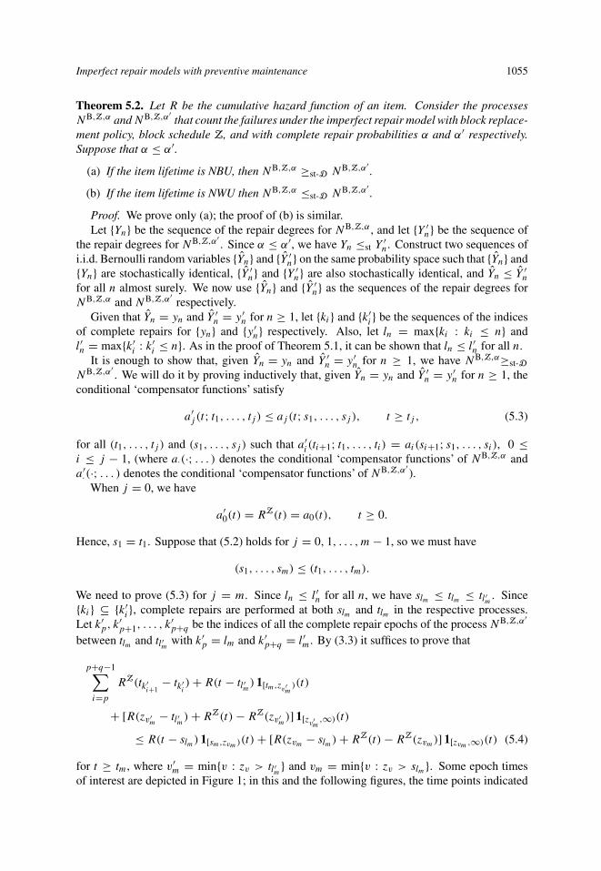
≤ R(t − slm) 1[sm,zvm)(t) + [R(zvm − slm) + RZ(t) − RZ(zvm)] 1[zvm ,∞)(t) (5.4)

for t ≥ tm, where v′m = min{v : zv > tl′m} and vm = min{v : zv > slm}. Some epoch times

of interest are depicted in Figure 1; in this and the following figures, the time points indicated


NB,Z,αslm t

NB,Z,α′tlm tk′p+1

tk′p+2 . . . tl′m tm t

Figure 1: Time points of interest.

NB,Z,αslm t zvm

NB,Z,α′tlm tk′p+1

tk′p+2 . . . tl′m tm t zv′

m

Figure 2: Case 1(a)(I).

NB,Z,αslm zvm t zv′

m

NB,Z,α′tlmtk′

p+1tk′

p+2 . . . tl′m tm t zv′m

Figure 3: Case 1(a)(II).

on the top line are associated with the process NB,Z,α′, whereas the time points indicated on

the bottom line are associated with the process NB,Z,α . Note that in the computations in theanalysis that follows, no complete repairs occur during the time interval (tl′m, t) in the processNB,Z,α′

, and no complete repairs occur during the time interval (slm, t) in the process NB,Z,α .

We prove (5.4) by considering various cases.

Case 1. zi /∈ [tlm, tl′m ] for all i.(a) t ≤ zv′

m.

(I) t ≤ zvm . Here we have zv′m

= zvm (see Figure 2). It follows from the fact that theunderlying component lifetime is NBU and since slm ≤ tlm that

p+q−1∑

i=p

RZ(tk′i+1

− tk′i) + R(t − tl′m) ≤ R(t − tlm)

≤ R(t − slm),

and (5.4) holds.

(II) t > zvm . Here slm < zvm < tlm because there are no block maintenance epochs in[tlm, t] (see Figure 3). Thus, using the fact that the underlying component lifetimeis NBU, as in Case 1(a)(I) we have

p+q−1∑

i=p

RZ(tk′i+1

− tk′i) + R(t − tl′m) ≤ R(t − tlm)

≤ RZ(t) − RZ(zvm),

and (5.4) holds.


NB,Z,αslm zvm t

NB,Z,α′tlmtk′

p+1tk′

p+2 . . . tl′m tm zv′m t

Figure 4: Case 1(b)(I).

NB,Z,αslm zvm zv′

mt

NB,Z,α′tlmtk′

p+1tk′

p+2 . . . tl′m tm zv′m t

Figure 5: Case 1(b)(II).

(b) t > zv′m.

(I) zvm = zv′m. This case is depicted in Figure 4. Since there are no block replacement

epochs in [tlm, zv′m], the NBU assumption yields

p+q−1∑

i=p

RZ(tk′i+1

− tk′i) + R(zv′

m− tl′m) + RZ(t) − RZ(zv′

m)

≤ R(zv′m

− tlm) + RZ(t) − RZ(zv′m)

≤ R(zvm − slm) + RZ(t) − RZ(zvm),

and (5.4) holds.

(II) zvm �= zv′m. Here slm < zvm < tlm (see Figure 5). Using the NBU assumption, we

havep+q−1∑

i=p

RZ(tk′i+1

− tk′i) + R(zv′

m− tl′m) + RZ(t) − RZ(zv′

m)

≤ R(zv′m

− tlm) + RZ(t) − RZ(zv′m)

≤ RZ(t) − RZ(zvm),

and (5.4) holds.

Case 2. zi ∈ [tlm, tl′m ] for some i. Note that here t ≥ zvm .

(a) zvm ∈ [tlm, tl′m ]. This case is depicted in Figure 6. Here, from the fact that the underlyingcomponent lifetime is NBU, we get

p+q−1∑

i=p

RZ(tk′i+1


m)(t)

+ [R(zv′m

− tl′m) + RZ(t) − RZ(zv′m)] 1[zv′

m,∞)(t)

≤ R(zvm − slm) + RZ(t) − RZ(zvm),

and (5.4) holds.


NB,Z,αslm zvm t

NB,Z,α′tlmtk′

p+1tk′

p+2 . . . zvm . . . tl′m tm t

Figure 6: Case 2(a).

NB,Z,αslm zvm z′ z′′ t

NB,Z,α′tlmtk′

p+1tk′

p+2 . . . . . . tl′m tm t

Figure 7: Case 2(b).

(b) zvm ∈ [slm, tlm ]. Let z′ = max{zn : zn ≤ tlm} and z′′ = min{zn : zn > tlm} (see Figure 7).Then, since the underlying component lifetime is NBU, we obtain

p+q−1∑

i=p

RZ(tk′i+1


m)(t)

+ [R(zv′m

− tl′m) + RZ(t) − RZ(zv′m)] 1[zv′

m,∞)(t)

≤ R(z′′ − z′) + RZ(t) − RZ(z′′)≤ R(zvm − slm) + RZ(t) − RZ(zvm),

and (5.4) holds.

Summarizing, we have shown that (5.4) holds, and thus (5.3) holds for all j . ByTheorem2.1,NB,Z,α′ ≤st-D NB,Z,α given that Yn = yn and Y ′

n = y′n forn ≥ 1. Byunconditioning, we obtain

NB,Z,α′ ≤st-D NB,Z,α .

It is of interest to note some relationships between Theorem 5.2 and results of Last andSzekli (1998).

Firstly, the reader may wonder whether Theorem 5.2 can be extended to the case in which,upon failure, the repair degrees Yn are more general than the Bernoulli random variables thatare assumed in Theorem 5.2 (and throughout the paper). This corresponds to the assumptionthat the virtual age after a repair (see Remark 3.1) can be more general than just being zeroor unchanged. For the model without any preventive maintenance, Last and Szekli (1998,Theorem 3.1) showed that, if the NBU assumption in Theorem 5.2(a) is replaced by the strongerassumption of IFR, then the conclusion of Theorem 5.2(a) holds for the more general repairdegrees Yn. By applying Theorem 3.1 of Last and Szekli (1998) to each block replacementinterval, and putting these intervals together via an independence assumption, it is seen that,under the IFR assumption, the conclusion of Theorem 5.2(a) holds for general stochasticallyordered repair degrees.

Secondly, Last and Szekli (1998, Remark 3.2) noted that, for Bernoulli Yn, in the modelwithout any preventive maintenance, the conclusion of our Theorem 5.2(a) can indeed beobtained under the assumption of NBU (rather than the IFR assumption in Theorem 3.1 of Last


and Szekli (1998)). Thus, by applying this observation to each block replacement interval,and putting these intervals together via an independence assumption, an alternative proof ofour Theorem 5.2(a) can be obtained. It should be noted, however, that Last and Szekli (1998)provided no proof for the statement in their Remark 3.2.

Acknowledgements

We thank a referee for some illuminating comments that led to an improvement of thecontents and of the presentation of this paper. The first author was supported in part by NSFgrant DMI 9812994.

References

Abdel-Hameed, M. (1987). An imperfect maintenance model with block replacements. Appl. Stoch. Models DataAnal. 3, 63–72.

Barlow, R. E. and Proschan, F. (1975). Statistical Theory of Reliability and Life Testing. Holt, Rinehart andWinston,NewYork.

Berg, M. and Cléroux, R. (1982). The block replacement problem with minimal repair and random repair costs.J. Statist. Computation Simulation 15, 1–7.

Block, H.W., Langberg, N. A. and Savits, T. H. (1990a). Comparisons for maintenance policies involving completeand minimal repair. In Topics in Statistical Dependence (IMS Lecture Notes Monogr. 16), eds H. W. Block,A. R. Sampson and T. H. Savits, Inst. Math. Statist., Hayward, CA, pp. 57–68.

Block, H. W., Langberg, N. A. and Savits, T. H. (1990b). Maintenance comparisons: block policies. J. Appl. Prob.27, 649–657.

Brown, M. and Proschan, F. (1983). Imperfect repair. J. Appl. Prob. 20, 851–859.Fontenot, R. A. and Proschan, F. (1984). Some imperfect maintenance models. In Reliability Theory and Models,

eds M. S. Abdel-Hameed, E. Çinlar and J. Quinn, Academic Press, San Diego, pp. 83–101.Kijima, M. (1989). Some results for repairable systems. J. Appl. Prob. 26, 194–203.Kwiecinski, A. and Szekli, R. (1991). Compensator conditions for stochastic ordering of point processes. J. Appl.

Prob. 28, 751–761.Last, G. and Szekli, R. (1998). Stochastic comparison of repairable systems by coupling. J. Appl. Prob. 35, 348–370.Li, H. and Xu, S. (2001). On the Markov block replacement policy in multivariate repairable systems. To appear in

Operat. Res.Pham, H. and Wang, H. (1996). Imperfect maintenance. Europ. J. Operat. Res. 94, 425–438.Rolski, T. and Szekli, R. (1991). Stochastic ordering and thinning of point processes. Stoch. Process. Appl. 37,

299–312.Shaked, M. and Szekli, R. (1995). Comparison of replacement policies via point processes. Adv. Appl. Prob. 27,

1079–1103.Wang, H. (2002). A survey of maintenance policies of deteriorating systems. Europ. J. Operat. Res. 139, 469–489.

Imperfect repair models with preventive maintenance

Documents

Transcript of Imperfect repair models with preventive maintenance