4-40

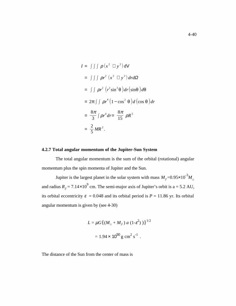
I = I I I ρ x 2 + y2 d V

= I I I ρ r 2 x 2 + y2 drdΩ

= I I ρ r 2 r 2 sin2 θ dr sinθ d θ

= 2 π I I ρ r 4 1 − cos2 θ d cos θ dr

= 8 π 3

I ρ r 4 dr= 8 π 15

ρ R 5

= 2 5

MR2 .

4.2.7 Total angular momentum of the Jupiter-Sun System

The total angular momentum is the sum of the orbital (rotational) angular

momentum plus the spin momenta of Jupiter and the Sun.

Jupiter is the largest planet in the solar system with mass MJ =0.95×10-3

Mu

and radius RJ = 7.14×109 cm. The semi-major axis of Jupiter’s orbit is a = 5.2 AU,

its orbital eccentricity ε = 0.048 and its orbital period is P = 11.86 yr. Its orbital

angular momentum is given by (see 4-30)

L = µG (Mu + MJ ) a (1-ε2) ) 1/2

= 1.94 × 1050 g cm2 s-1 .

The distance of the Sun from the center of mass is

4-41

au = aMJ

M J + M u

= 7.4 × 1010

cm

(slightly larger than the Sun’s radius). Assuming that the Sun moves in a circular

orbit, its angular momentum is

Lu = Mu vu au = M

u 2 π a 2

u

P

= 1.84 × 1047

g cm2 s

-1 .

(Note: Lu is not the solar luminosity here!)

The distance from Jupiter to the center of mass is aJ = a - au ~ a. So its angular

momentum is

LJ = M

J v

J a

J = M

J =

M u 2 π a 2

P

= 1.94 × 1050 cm2 s-1 .

So L = Lu + LJ (as it must).

The spin angular momentum of the Sun is

Lu

s

= Iuωu = Iu 2 π P u

= 4 π 5

M u R 2

u

P u .

Pu = 26 days, Ru = 6.696 × 105 km, M u = 1.99 × 10

33 g.

4-42

Lus = 9.9 × 1048 g cm2 s-1 .

Similarly, using PJ = 10 hours

LJ s = 6.7 × 1045 g cm2 s-1 .

Angular momentum of the Sun-Jupiter system is dominated by the orbital motion

but if the Sun were a rapidly rotating star, its spin could dominate.

4.3 Binary stars

(See Ostlie and Carroll, Chapter 7)

More than half the stars are multiple stars, most of which are binary pairs.

For solar-type stars, the observed ratios of single: double: triple: quadrupole

systems is 45:46:8:1. There are several classes of binaries:

visual binaries: both can be detected orbiting in ellipses about one another (Sirius

is a famous example - Sirius A is a main sequence star of spectral type A1, Sirius B

is a white dwarf of spectra type A5. The period is 49.9 years.

Sirius was first discovered as an astrometric binary.

Astrometric binaries are binaries in which only one star is observed but its

motion is oscillatory, indicating the perturbing presence of a dim companion.

Spectroscopic binaries are visually unresolved but periodic oscillations occur in

their spectrum. If only one stellar spectrum is observed, the binary is single-lined; if

both are observed, the binary is double-lined.

4-43

Eclipsing binaries occur when the two stars eclipse one another, producing

periodic changes in apparent brightness.

Periods of binary stars vary from a few hours to hundreds of years. From

data on the periods we can use the law of gravitation to infer masses. Consider a

double-lined spectroscopic binary. The spectra of the two stars are superimposed.

We can use Doppler shifts to measure the radial velocities of each star, even though

they may be too close for their orbits to be distinguished.

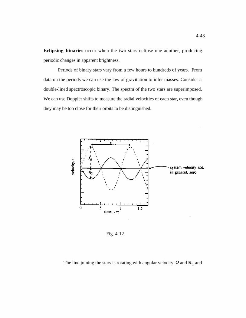
Fig. 4-12

The line joining the stars is rotating with angular velocity Ω and K1 and

4-44

K2 are the inferred radial velocities.

The figure shows the individual radial velocities. From it we obtain the

peak velocities of each star and the binary period τ. If the shape is accurately

sinusoidal, the orbits are circular with ε = 0. The distances r1 and r2 from the center

of mass are constant for circular orbits. The center of mass is the center of the

orbits of both stars and of their relative motion.

cm

r

2

r

1

M

2

Ω

r

2

M

1

Ω

r

1

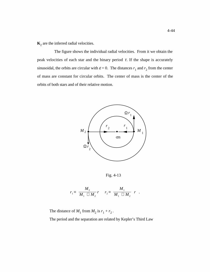
Fig. 4-13

r 1 = M 2

M 1 + M 2

r r 2 = M 1

M 1 + M 2

r .

The distance of M1 from M2 is r1 + r2 .

The period and the separation are related by Kepler’s Third Law

4-45

τ 2 = 4 π 2 r3

G M =

4 π 2 r1 + r 2

3

G M 1 + M 2

and the speeds of the stars are

v1 = Ωr1 , v2 = Ωr2

where Ω is the angular velocity

Ω = 2 π τ .

So r = r1 + r2 = (v1 + v2)/Ω

M 1

M 2

= r

2

r 1

= v

2

v 1

, independent of i

M 1 + M

2 = Ω 2 r 3

G .

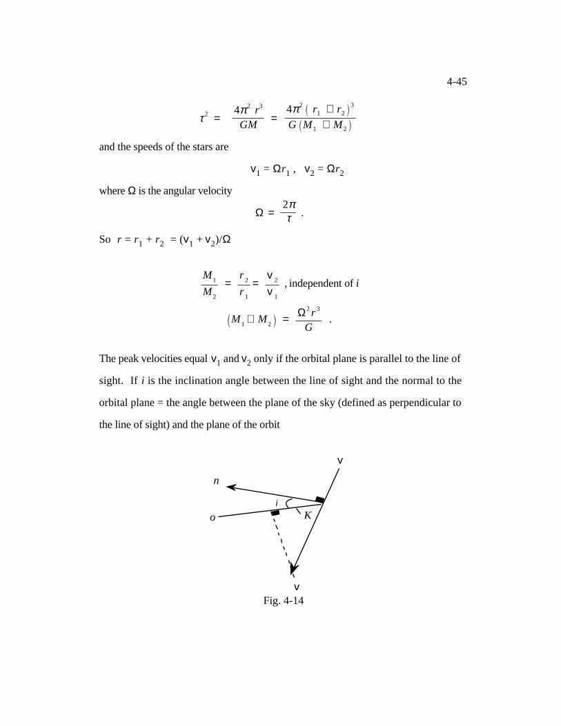
The peak velocities equal v1 and v2 only if the orbital plane is parallel to the line of

sight. If i is the inclination angle between the line of sight and the normal to the

orbital plane = the angle between the plane of the sky (defined as perpendicular to

the line of sight) and the plane of the orbit

i

n

o

v

K

v

Fig. 4-14

4-46

K1 = v1 sin i = Ωr1 sin i = 2 π τ r1 sin i

K2 = v2 sin i = Ωr2 sin i = 2 π τ r2 sin i

If i = 0, we observe zero velocities (no information). i = 90° is edge on

K1 =v1, K2 =v2. The mass ratio is in any case independent of i.

M 1

M 2

= K 2

K 1

= v 2

v 1

.

The separation r = r1 +r2 = τ K 1 + K 2

2 π sin i

The total mass we obtain from

M = Ω 2 r 3

G =

4 π 2

τ 2 r 3

G

M = M 1 + M2 = τ

2 π G K 1 + K 2

3

sin3 i .

Hence we may write for the case when only K2 can be measured,

4-47

M 1 + M 2 = τ

2 π G

1

sin3 i M 1 + M 2

3

M 3 1

K 3 2

M 1 + M 2 = τ

2 π G

1

sin3 i

1 +

M 2

M 1

3

K 3 2 .

If we write this equation in the form

τ 2 π G

K 3 2 =

M 1 sin i 3

M 1 + M 2 2 = f ( M )

we define a function f(M) called the mass function. The left-hand side depends only

on observable properties and is useful for statistical studies (Ostlie and Caroll p.

211).

We may write for the separate masses,

M 1 sin3 i = τ

2 π G K 1 + K 2

2 K 2

M 2 sin3 i = τ

2 π G K 1 + K 2

2 K 1

but in general we do not know i.

For eclipsing binaries, each star successively eclipses the other. To see them, i must

be near 90°, assuming that the stellar radii are much less than the stellar separation.

Masses are insensitive to i for i near 90° since sin i ~ 1.

4-48

t

a

t

b

t

c

a

b

c

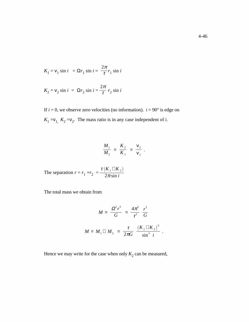
Fig. 4-15

From the duration of the eclipses we can infer the radii of the stars. Assume i =

90°. Let ta be the time of first contact of the primary eclipse and let tb be the time of

minimum light. During eclipses stars are moving nearly perpendicular to the line of

sight to the observer in opposite directions. Thus, if vs and vl are the velocities of

the small and large stars respectively, their relative velocity is vs + vl The radius of

the smaller star is given by

4-49

rs = 1 2

(vs + vl)(tb - ta)

and the radius of the larger star by

r l = 1 2

(vs + vl)(tc- tb)

where tc- tb is the duration of minimum light (see Ostlie and Carroll §7.1)

4.4 Extrasolar planets

It is primarily by velocity measurements of the parent star that extra solar

planets have been detected and we do not know the planet velocity. Let Ms be the

stellar mass and Mp the planetary mass. Suppose τ is the measured period and Ks

the measured stellar velocity. The mass function f (M) is

M p sin i 3

M p + M s 2 =

τ K 3 s

2 π G

If we assume Ms >> Mp,

M p sin i 3 =

τ K 3 s

2 π G M 2

s .

Observations of the star Peg A—a G star like the Sun—have revealed the existence

of a companion and τ and Ks have been measured. From them we get

4-50

Mp sin i = (1.36 × 1020 Ms2)1/3

The mass of Peg A is 0.95 Mu ~ 2 × 1030

kg so if sin i = 1

Mp = 8 × 1026 kg .

It is customary to express the mass of extra solar planets in Jupiter masses

Mp = 0.45 MJ .

The orbital radius is obtained from a = Ksτ / 2π

It equals 3000 km. From

a p

a -

M s

M p

,

we obtain for the distance of the planet from the star a value of 0.05 AU. The value

of Mp and ap depend on the assumption that i = 90°. Mp could be underestimated

and ap overestimated.

4.5 Supernovae in binary systems

Supernovae are exploding stars. Before explosion many occur as binary

systems and are caused by mass flow from a companion star. What happens to the

binary system when the explosion occurs and the mass of one star is reduced,

possibly to zero?

4-51

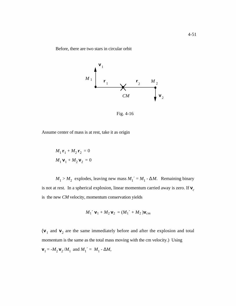
Before, there are two stars in circular orbit

M

CM

v 1

v 2

1r

2r

21 M

Fig. 4-16

Assume center of mass is at rest, take it as origin

M1 r 1 + M2 r 2 = 0

M1 v1 + M2 v2 = 0

M1 > M2 explodes, leaving new mass M1´ = M1 - ∆M. Remaining binary

is not at rest. In a spherical explosion, linear momentum carried away is zero. If vc

is the new CM velocity, momentum conservation yields

M1´ v1 + M2 v2 = (M1´ + M2 )vcm

(v 1 and v2 are the same immediately before and after the explosion and total

momentum is the same as the total mass moving with the cm velocity.) Using

v1 = -M2 v2 /M1 and M1´ = M1 - ∆M,

4-52

(M1 - ∆M)

− M 2

M 1

v 2

+ M2 v2

= (M1 - ∆M + M2 )vcm

giving

v cm

= ∆ M M

2

M 1 M

1 + M

2 − ∆ M

v 2 .

If ∆M = M1, vc = v2 (as it must).

Typical values are M1= 10 Mu , M2 = 5 Mu , ∆M = 8.5 Mu . Then M1´ =

1.5 Mu (appropriate for a neutron star).

v cm

= 8 . 5 x 5 10 x 5 . 5

v 2 = 0 . 77 v

2 .

For close binaries, v2 may be several hundred km s-1

so system really moves.

To determine whether or not the binary remains bound, calculate the binding

energy, that is, the internal energy without the center of mass energy.

The total internal energy of the system immediately after the explosion is

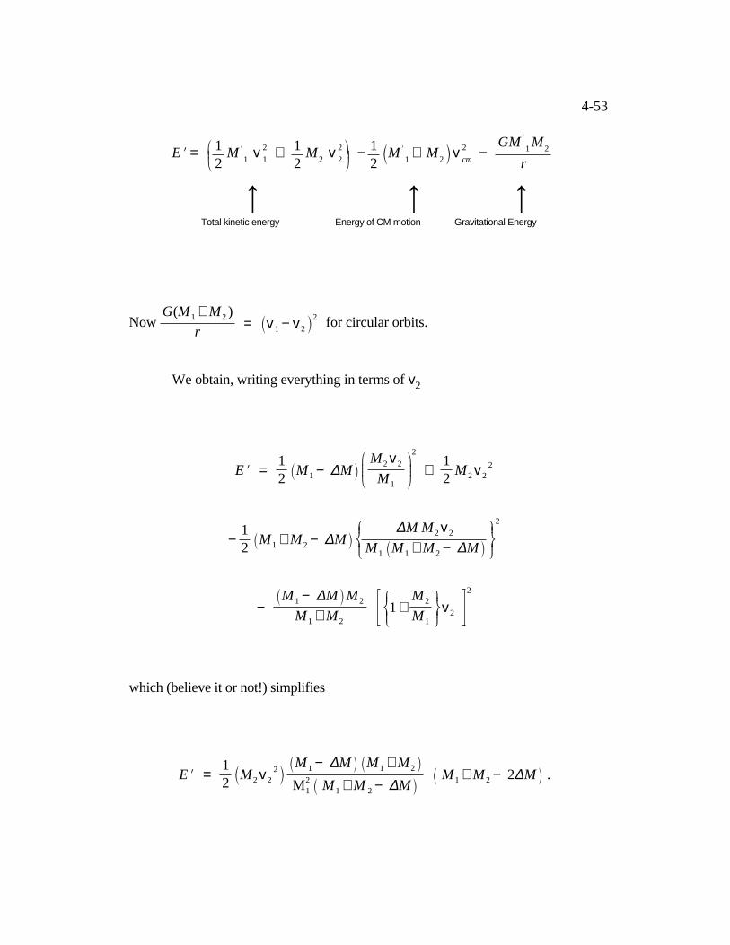
4-53

E N = 1 2

M N 1 v 2

1 + 1

2 M

2 v 2

2 − 1

2 M N

1 + M

2 v 2

cm −

G M N 1 M

2

r

8 8 8 Total kinetic energy Energy of CM motion Gravitational Energy

Now G ( M 1 + M 2 )

r = v 1 − v 2

2 for circular orbits.

We obtain, writing everything in terms of v2

E N = 1 2 M 1 − ∆ M

M 2 v 2

M 1

2

+ 1 2

M 2 v 2 2

− 1 2 M 1 + M 2 − ∆ M

: ; <

= =

= = ∆ M M 2 v 2

M 1 M 1 + M 2 − ∆ M

B C D

E E

E E

2

− M 1 − ∆ M M 2

M 1 + M 2

: ; <

= = = 1 +

M 2

M 1

B C D

E E E v 2

2

which (believe it or not!) simplifies

E N = 1 2 M 2 v 2

2 M 1 − ∆ M M 1 + M 2 M 2

1 M1 + M 2 − ∆ M M1 + M 2 − 2 ∆ M .

4-54

All terms are positive except the last factor.

Thus for E´ to be positive (no binding) , mass ejected ∆M > 1/2 (M1 + M2).

In the numerical example on p 4.52

8.5 > 1 2

(10 + 5)

and the neutron star departs at high velocity.

Pulsars (rotating neutron stars) often have high velocity as they leave the

galactic plane.

The result can be obtained more readily using the CM system in which the

total energy is

Etot = 1 2

M v2cm + µ (

1 2

v2 -GM/r)

where v is the relative velocity. Before the explosion for the initial circular orbit

v 2 = GMr

and

E µ

= 1 2

v 2 − GMr

= − GM2 r

.

(see page 4-29) where E is internal energy.

4-55

After explosion, v is unchanged—µ, M and E change as M changes to M´ . Internal

energy is changed from 1 2

v 2 − GM

r to

E µ N

= 1 2

v 2 − GMN r

= GM2 r

− GMN r

.

So internal energy > 0 if M´ < M/2 and ejected mass ∆ M > M/2.

4.6 Tides

When two bodies are in orbit around each other, the otherwise spherically

symmetric gravitational field is distorted by the gravitational attraction of the other

body. The force field can be characterized by equipotentials which are like contours

of height on a map; the force is zero tangent to the equipotential surface and is

normal everywhere to the surface.

4-56

4.6.1 Weak tides1111111111111111111111111111111111111111

000000000000000000000000000000000000000011111111111111111111111111111111

00000000000000000000000000000000

11111111111111111111

00000000000000000000

1111111111111111111111111111

0000000000000000000000000000

Earth

Moon

R

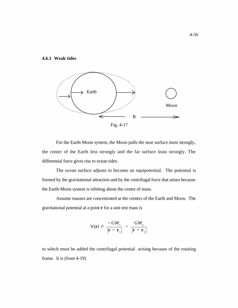
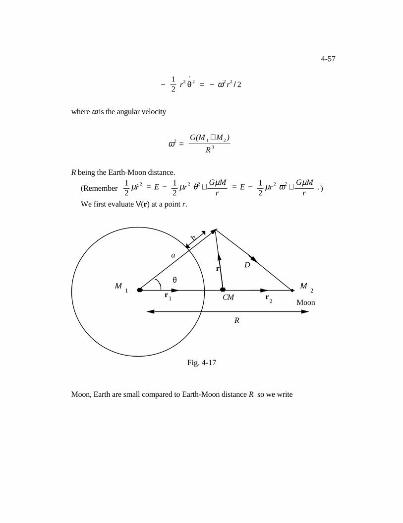
Fig. 4-17

For the Earth-Moon system, the Moon pulls the near surface most strongly,

the center of the Earth less strongly and the far surface least strongly. The

differential force gives rise to ocean tides.

The ocean surface adjusts to become an equipotential. The potential is

formed by the gravitational attraction and by the centrifugal force that arises because

the Earth-Moon system is orbiting about the center of mass.

Assume masses are concentrated at the centers of the Earth and Moon. The

gravitational potential at a point r for a unit test mass is

V ( r ) = − GM

1

r − r 1

− GM

2

r − r 2

to which must be added the centrifugal potential arising because of the rotating

frame. It is (from 4-19)

4-57

− 1 2

r 2 .

θ 2 = − ω 2 r 2 / 2

where ω is the angular velocity

ω 2 = G ( M 1 + M 2 )

R 3

R being the Earth-Moon distance.

(Remember 1 2

µ r 2 = E − 1 2

µ r 2 θ ˙ 2 + G µ M r

= E − 1 2

µ r 2 ω 2 + G µ M r

.)

We first evaluate V(r ) at a point r.

Moon

θ

a

CM

R

r

D

r

2

r

1

Μ

2

Μ

1

b

Fig. 4-17

Moon, Earth are small compared to Earth-Moon distance R so we write

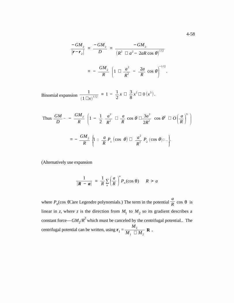
4-58

− GM2

r − r 2

= − GM

2

D =

− GM2

R 2 + a2 − 2 aR cos θ 1 / 2

= − GM

2

R

1 + a

2

R 2 − 2 a

R cos θ

− 1 / 2

.

Binomial expansion 1

1 + x 1 / 2

= 1 − 1 2

x + 3 8

x 2 + 0 x 3 .

Thus GMD

- − GM

2

R

1 − 1

2 a

2

R 2 + a

R cos θ + 3 a 2

2 R 2 cos θ 2 + O

a R

3

= − GM

2

R : ; <

= = = 1 + a

R P

1 cos θ + a2

R 2 P

2 cos θ + ...

B C D

E E E .

(Alternatively use expansion

1 R − a

= 1 R 3 n

a R

n

P n ( cos θ ) R > a

where Pn(cos θ) are Legendre polynomials.) The term in the potential a R cos θ is

linear in z, where z is the direction from M1 to M2 so its gradient describes a

constant force—GM2/R2

which must be canceled by the centrifugal potential.. The

centrifugal potential can be written, using r1 = M 2

M 1 + M 2

R ,

4-59

− 1 2

ω 2 r 2 = 1 2

ω 2 r 1 − a 2 = 1

2 ω 2 r

2

1 + a2 − 2 r

1 a cos θ

= 1 2

ω 2

M

2

M 1 + M

2

R 2 + a2 −

2 M 2

M 1 + M

2

R a cos θ .

So adding this we have for the total potential Φ(r)

Φ ( r ) = − GM1

a −

GM2

R 1 +

a R

cos θ + 1 / 2 ( 3 cos2 θ − 1 ) a 2

R 2

− 1 2

G M 1 + M 2

R 3

M 2

M 1 + M 2

2

R 2 + a 2 − 2

M 2

M 1 + M 2

R a cos θ .

The term in a R cos θ is indeed canceled out by the centrifugal force that keeps the

body in a circular orbit. The gradient of terms that do not depend on a or θ is zero,

so they may be omitted and we have for the local tidal potential

Φ ( r ) = − GM1

a −

1 2

Ga2

R 3 3 M 2 cos2 θ + M 1 .

Expand a in terms of its height above the mean sea level a = Rr + h. Then

4-60

a 2 Rr

2

1 + 2 h

Rr

,

a − 1 Rr

1 − h

Rr

and

Φ ( h , θ ) = − GM

1

R r

1 − h

R r

− 1

2

G R 2

r

R 3

1 + 2 h

R r

3 M

2 cos2 θ + M

1

- GM

1

R r

2 h − 3

2

M

2

M 1

R

r

R

3

R r cos2 θ

ignoring constant terms.

GM1

R r 2 = g = acceleration due to gravity at the surface of the Earth.

The surface will adjust to be an equipotential (the tangential force vanishes) so

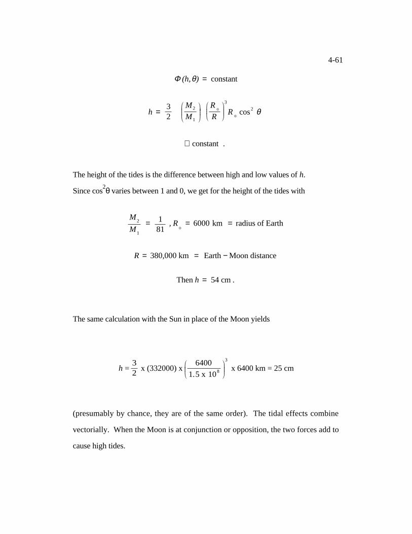
4-61

Φ ( h , θ ) = constant

h = 3 2

M 2

M 1

R r R

3

R r cos2 θ

+ constant .

The height of the tides is the difference between high and low values of h.

Since cos2θ varies between 1 and 0, we get for the height of the tides with

M 2

M 1

= 1 81

, Rr = 6000 km = radius of Earth

R = 380, 000 km = Earth− Moon distance

Then h = 54 cm .

The same calculation with the Sun in place of the Moon yields

h = 3 2

x (332000) x

6400

1 . 5 x 108

3

x 6400 km = 25 cm

(presumably by chance, they are of the same order). The tidal effects combine

vectorially. When the Moon is at conjunction or opposition, the two forces add to

cause high tides.

4-62

4.6.2 Tidal friction

The continents are pulled through the ocean bulges and the tidal bulge is

dragged ahead by the spinning Earth. There is a loss of energy by friction and the

spin of the Earth is slowed. The day is getting longer. (There is evidence from

growth scales in fossil corals that there were 400 days in a year about 100 million

years ago). Angular momentum is conserved so the Moon increases its angular

momentum. It can do so because the non-symmetric bulge creates a gravitational

torque back on the Moon. Increasing the angular momentum means the Moon

must move outward ( r o = L2/Gmµ2

, a =

r o

( 1-ε 2 ) ) and so the month is getting

longer. The lowest energy state of the Moon-Earth system is one in which the Earth

and Moon present the same face—in which case the tidal distortion will have

reached its equilibrium shape that involves no relative motion of any material. The

Earth and Moon will be tidally locked and there will be no drag. The tidal bulge will

point directly at the Moon and the Earth and the Moon will corotate.

Because the Moon is not exactly spherical, partial locking has already

occurred, in that the Moon rotates with the Earth so that it shows the same face all

the time. The Moon is in synchronous rotation such that the orbital period of the

Moon around the Earth equals the rotation or spin period of the Moon. The

ultimate equilibrium caused by tidal friction is that in which the spin velocity of the

Earth equals the angular velocity of the Moon in orbit around the Earth (or the

angular velocity of the Earth about the moon) so that 1 month equals 1 day.

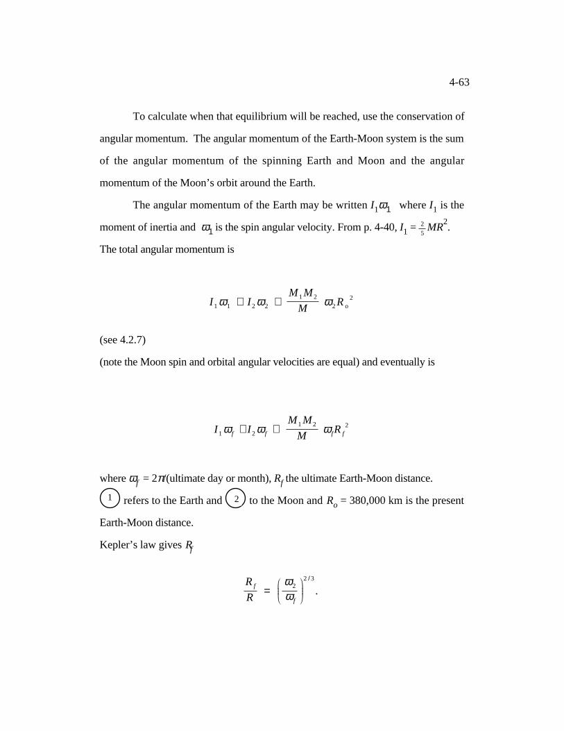
4-63

To calculate when that equilibrium will be reached, use the conservation of

angular momentum. The angular momentum of the Earth-Moon system is the sum

of the angular momentum of the spinning Earth and Moon and the angular

momentum of the Moon’s orbit around the Earth.

The angular momentum of the Earth may be written I1ω1 where I1 is the

moment of inertia and ω1 is the spin angular velocity. From p. 4-40, I1 = 2

5 MR

2.

The total angular momentum is

I 1 ω 1 + I 2 ω 2 + M 1 M 2

M ω 2 R o

2

(see 4.2.7)

(note the Moon spin and orbital angular velocities are equal) and eventually is

I 1 ω f + I 2 ω f + M 1 M 2

M ω f R f

2

where ωf = 2π/(ultimate day or month), Rf the ultimate Earth-Moon distance.

1

1 refers to the Earth and

1

2 to the Moon and Ro = 380,000 km is the present

Earth-Moon distance.

Kepler’s law gives Rf

R f R

=

ω 2

ω f

2 / 3

.

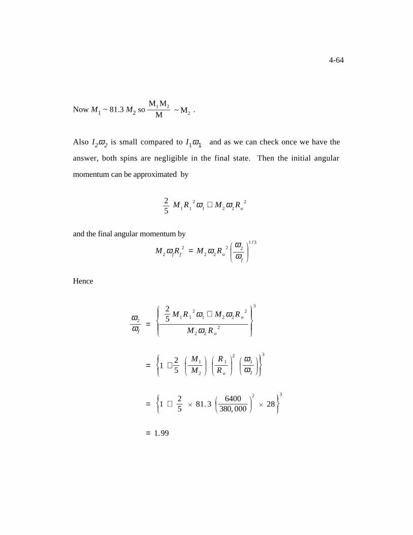
4-64

Now M1 ~ 81.3 M2 so M 1 M 2

M ~ M 2

.

Also I2ω2 is small compared to I1ω1 and as we can check once we have the

answer, both spins are negligible in the final state. Then the initial angular

momentum can be approximated by

2 5

M1 R

1

2 ω 1

+ M 2 ω

2 R

o

2

and the final angular momentum by

M 2 ω

f R

f

2 = M 2 ω

2 R

o

2

ω

2

ω f

1 / 3

Hence

ω 2

ω f =

:

;

<

= = = = =

= = = = =

2 5

M 1 R 1 2 ω 1 + M 2 ω 2 R o

2

M 2 ω 2 R o 2

B

C

D

E E E E E

E E E E E

3

= : ; <

= =

= = 1 + 2 5

M1

M2

R1

R o

2

ω 1

ω 2

B C D

E E

E E

3

= : ; <

= = 1 +

2 5

H 81. 3

6400380, 000

2

H 28B C D

E E

3

= 1 . 99

4-65

The final length of the day and month will be 28 x 1.99 = 54 days.

The current lengthening of the day is about 0.2 days in 109 years so it will

take more than 1010

years to reach equilibrium. (We will have been engulfed by the

Sun in its evolution by then).

The same tidal forces bring binary stars into corotation, tidally locked to

each other.

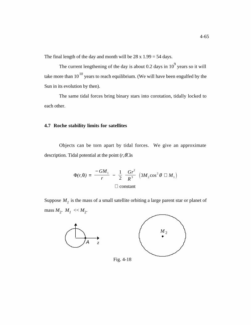
4.7 Roche stability limits for satellites

Objects can be torn apart by tidal forces. We give an approximate

description. Tidal potential at the point (r,θ) is

Φ ( r , θ ) = − GM1

r −

1 2

Gr2

R 3 3 M 2 cos2 θ + M 1

+ constant

Suppose M1 is the mass of a small satellite orbiting a large parent star or planet of

mass M2. M1 << M2.

M

2

Α

z

Fig. 4-18

4-66

Calculate the force at point A. If it points towards the center of the satellite, it is a

restoring force. If it points away towards M2, the satellite is torn apart.

Gravitational acceleration along the z axis at A is given by

g z = − L z Φ = − d dz

− GM1

z −

1 2

Gz2

R 3 3 M 2

= − GM1

z 3 z + z3 GM2

R 3

= Gz

−

M 1

z 3 + 3 M 2

R 3

.

The condition for Roche stability is

M 1

r 3 >

3 M 2

R 3

Putting |z|=r, for a satellite of mean density ρ we obtain

ρ > 9 4 π

M

2

R 3

or no satellite of density ρ is stable inside the Roche radius Rcrit. The critical radius

is

4-67

R crit

=

9 M

2

4 π ρ

1 / 3

.

If the parent (planet) and satellite have same density

R crit = 3 1 / 3 R 2 = 1 . 44 R2

where R2 is radius of the parent. (Roche calculated 2.44 R2 using a model of the self-

gravity of the satellite).

This is essentially the physics of the rings of Saturn (and other planets).

Material within the Roche limit cannot form bodies such as moons because of the

disruptive effect of tidal forces.

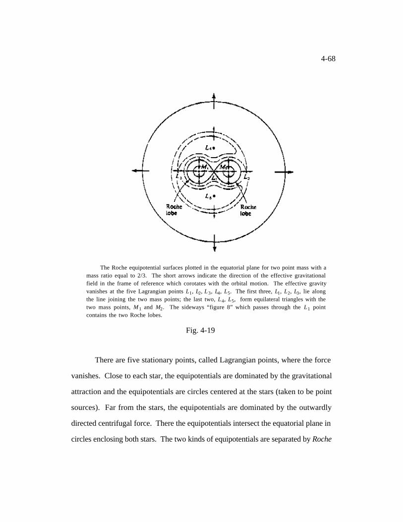
4.8 Roche lobes

Consider a binary stellar system in a circular orbit. The intersections of the

equipotential surfaces with the plane of the orbit are shown in the Figure. (See Ostlie

and Caroll p. 687).

4-68

The Roche equipotential surfaces plotted in the equatorial plane for two point mass with amass ratio equal to 2/3. The short arrows indicate the direction of the effective gravitationalfield in the frame of reference which corotates with the orbital motion. The effective gravityvanishes at the five Lagrangian points L1, L2, L3, L4, L5. The first three, L1, L2, L3, lie alongthe line joining the two mass points; the last two, L4, L5, form equilateral triangles with thetwo mass points, M1 and M2. The sideways “figure 8” which passes through the L1 pointcontains the two Roche lobes.

Fig. 4-19

There are five stationary points, called Lagrangian points, where the force

vanishes. Close to each star, the equipotentials are dominated by the gravitational

attraction and the equipotentials are circles centered at the stars (taken to be point

sources). Far from the stars, the equipotentials are dominated by the outwardly

directed centrifugal force. There the equipotentials intersect the equatorial plane in

circles enclosing both stars. The two kinds of equipotentials are separated by Roche

4-69

lobes around each star indicated by the figure of eight. The Roche lobes intersect at

a saddle point, forming in a pitcher-like shape.

Roche lobes can be used to further classify close binaries. If both stars are

smaller than their Roche lobes, the system is a detached binary. If one fills its

Roche lobe, the system is a semi-detached binary and matter will flow through the

contact point. If both stars fill their Roche lobes they are contact binaries and they

have a common envelope.

The Roche lobe is the maximum possible size of the star. If a star of mass

M1 becomes larger than its Roche lobe, it overflows and dumps mass through the

saddle-point on to the companion star. A common scenario is the case where M1 is

initially much larger than M2 (possibly also losing mass to infinity in a stellar

wind). Mass flows from M1 to M2. Eventually M1 becomes a white dwarf and

cools. M2 has gained mass and so it evolves faster and overflows back on to M1.

This process manifests itself in an X-ray source. As the white dwarf accumulates

mass, it may be forced into a gravitational collapse to a neutron star in a supernova

explosion.

4.8.1 Effect of mass transfer on binary orbits

Suppose M1 is filling its Roche lobe and dumping mass on to M2. Mass

and angular momentum are conserved but not energy. The mass is heated and

dissipates energy in radiation.

M2 is gaining mass so M ˙ 2 = − M ˙

1 > 0 . The angular momentum for a

4-70

circular orbit

L = µ R 2 ω = µ R 2

GM

R 3

1 / 2

= M 1 M 2

M 1 / 2 R 1 / 2 G 1 / 2 = M 1 M 2 R 1 / 2 G 1 / 2 M − 1 / 2

0 = dLd t

= G 1 / 2 M − 1 / 2

. M 1 M 2 R 1 / 2 + M 1

. M 2 R 1 / 2

+ G 1 / 2 M − 1 / 2 1 2

M 1 M 2 R .

R − 1 / 2 .

Solving for R .

and eliminating M .

1 in favor of M .

2 , we obtain

. R = 2 R

M 2 − M 1

M 1 M 2

. M 2 .

If the lighter star M1 is losing mass R ˙ > 0 and stars draw apart. Often this

terminates the mass flow since it puts M1 deeper into its Roche lobe. Alternatively

the mass transfer proceeds slowly on the stellar evolutionary time scale that it takes

M1 to fill its increasingly large Roche lobe.

If the heavier star is losing mass R is negative. The stars get nearer which

4-71

increases mass flow leading to a catastrophic instability. In practice friction leads to

a merger of the two stars.

4.9 The Virial Theorem

Here I prove a useful theorem, the virial theorem.

Introduce

I = 1 2

N

3 i = 1

m i r i 2

(similar to moment of inertia but about a point).

The kinetic energy of N interacting particles of masses mi and velocities vi is

T = 1 2

N

3 i = 1

m i v i 2

The gravitational potential energy is

V = − 3 3 j

G m i m j r i − r j

Newton’s law

m i v ˙ i = − L i V

4-72

Differentiate I with respect to time twice

.

I = N

3 i = 1

m i v i A r i

..

I = N

3 i = 1

m i v ˙ i A r i + N

3 i = 1

m i v i A vi

= − 3 i

r i A L i V + 2 T .

This is the time-dependent virial theorem. To evaluate

3 i

r i A L i V

consider the scaled potential V(λr i ) obtained by replacing all position vectors by

λr i =ρρρρi, say. Then dρρρρi/dλ = r i and

d d λ V λ r i =

d d λ V ρρρρ i =

d V ρρρρ i d ρρρρ i

d ρρρρ i d λ = L i V A r i .

Thus

4-73

d d λ V λ r = 3

i

r i A L i V .

For a gravitational potential

V λ r = 1 λ V r

so

3 i

r i A L

i V = − 1

λ 2 V r .

Put λ = 1. Then

− 3 i

r i A L i V = V r

and

..

I = V + 2 T .

(See Ostlie and Carroll pp. 53-56.)

If a gravitational system is in equilibrium, neither increasing or decreasing in

size, it must have the long time average values < V > and <T > such that

< V + 2T> = 0 , < V > = -2 <T > .

We can prove this by averaging over a long time Γ

4-74

V + 2 T = 1 Γ

Γ

I 0 V + 2 T ) dt

= 1 Γ I Γ − I 0

If Γ is the orbital period, .

I ( T ) = .

I ( 0 ) . More generally, if all particles remain

bounded with bounded velocities for all time, I(t) remains bounded and the right-

hand side tends to zero. (This relationship <2T> = -< V> applies also to the

kinetic and potential energies of many electron atomic systems bound by the

Coulomb attraction between the nucleus and the electrons and can be established

using quantum mechanics.)

(For a harmonic oscillator, V ~ r2 ,

V(λr ) ~ λ2V(r )

d d λ V(λr ) = 2λV(r )

− 3 i

r i V

i V = 2 V ( r )

λ = 1..

I = -2V + 2T

<T> = <V> )

For an alternative proof of the Virial Theorem see Ostlie and Carroll,pp. 53-56.

4-75

4.10 Gravitational Collapse

Imagine a cloud mass M, uniform density ρ, radius ro

M = 4 3

π r 3 o ρ

held at r = ro and released. In the absence of other forces, cloud will collapse.

Conservation of energy

1 2

r . 2 =

GMr

− GMr o

tff =

t f f

I 0

dt = −

r o

I 0

dtdr

dr

=

r o

I 0

2 GM

r −

2 GMr o

− 1 / 2

dr .

Substitute x = r/r o

4-76

tff =

r 3 o

2 GM

1 / 2 1

I 0

x

1 − x

1 / 2

dx .

Put x = sin2θ; integral is π/2.

t ff =

3 π 32G ρ

1 / 2

, depending only on ρ .

Collapse time is independent of initial size.

For Sun, ρ=1.4 gm cm-3

tff = 1.8 x 103 sec = 30 minutes.