High-order kernels for Riemannian wavefield … P. Sava and S. Fomel ρ = c 2 b a 2. (19) In the...

Geophysical Prospecting, 2008, 56, 49–60 doi:10.1111/j.1365-2478.2007.00660.x

High-order kernels for Riemannian wavefield extrapolation

Paul Sava1∗ and Sergey Fomel21Centre for Wave Phenomena, Geophysics Department, Colorado School of Mines, Golden, CO 80401, USA, and 2Bureau of EconomicGeology, The University of Texas at Austin, Austin, TX 78713, USA

Received August 2006, revision accepted May 2007

ABSTRACTRiemannian wavefield extrapolation is a technique for one-way extrapolation ofacoustic waves. Riemannian wavefield extrapolation generalizes wavefield extrap-olation by downward continuation by considering coordinate systems different fromconventional Cartesian ones. Coordinate systems can conform with the extrapolatedwavefield, with the velocity model or with the acquisition geometry.

When coordinate systems conform with the propagated wavefield, extrapolationcan be done accurately using low-order kernels. However, in complex media or incases where the coordinate systems do not conform with the propagating wavefields,low order kernels are not accurate enough and need to be replaced by more accurate,higher-order kernels. Since Riemannian wavefield extrapolation is based on factoriza-tion of an acoustic wave-equation, higher-order kernels can be constructed using meth-ods analogous to the one employed for factorization of the acoustic wave-equationin Cartesian coordinates. Thus, we can construct space-domain finite-differences aswell as mixed-domain techniques for extrapolation.

High-order Riemannian wavefield extrapolation kernels improve the accuracy ofextrapolation, particularly when the Riemannian coordinate systems does not closelymatch the general direction of wave propagation.

I N T R O D U C T I O N

Riemannian wavefield extrapolation (Sava and Fomel 2005)generalizes solutions to the Helmholtz equation in Rieman-nian coordinate systems. Conventionally, the Helmholtz equa-tion is solved in Cartesian coordinates which represent specialcases of Riemannian coordinates. The main requirements im-posed on the Riemannian coordinate systems are that theymaintain orthogonality between the extrapolation coordinateand the other coordinates (2 in 3D, 1 in 2D). This requirementcan be relaxed when using an even more general form of Rie-mannian wavefield extrapolation in non-orthogonal coordi-nates (Shragge 2007). In addition, it is desirable that the coor-dinate system does not triplicate, although numerical methodscan stabilize extrapolation even in such situations (Sava and

∗E-mail: [email protected]

Fomel 2005). Thus, wavefield extrapolation in Riemanniancoordinates has the flexibility to be used in many applicationswhere those basic conditions are fulfilled. Cartesian coordi-nate systems, including tilted coordinates, are special cases ofRiemannian coordinate systems.

Two straightforward applications of wave propagation inRiemannian coordinates are extrapolation in a coordinate sys-tem created by ray tracing in a smooth background velocity(Sava and Fomel 2005) and extrapolation with a coordinatesystem created by conformal mapping of a given geometryto a regular space, for example migration from topography(Shragge and Sava 2005).

Coordinate systems created by ray tracing in a backgroundmedium often represent well wavefield propagation. In thiscontext, we effectively split wave propagation effects into twoparts: one part accounting for the general trend of wave prop-agation, which is incorporated into the coordinate system, andthe other part accounting for the details of wavefield scattering

C© 2007 European Association of Geoscientists & Engineers 49

50 P. Sava and S. Fomel

due to rapid velocity variations. If the background medium isclose to the real one, the wave-propagation can be properlydescribed with low-order operators. However, if the back-ground medium is far from the true one, the wavefield departsfrom the general direction of the coordinate system and thelow-order extrapolators are not enough for accurate descrip-tion of wave propagation.

For a coordinate system describing a geometrical propertyof the medium (e.g. migration from topography), there is noguarantee that waves propagate in the direction of extrapola-tion. This situation is similar to that of Cartesian coordinateswhen waves propagate away from the vertical direction, ex-cept that conformal mapping gives us the flexibility to defineany coordinates, as required by acquisition. In this case, too,low-order extrapolators are not enough for accurate descrip-tion of wave propagation.

Therefore, there is a need for higher-order Riemannianwavefield extrapolators in order to correctly handle wavespropagating obliquely relative to the coordinate system. Usu-ally, the high-order extrapolators are implemented as mixedoperators, part in the Fourier domain using a referencemedium, part in the space domain as a correction from thereference medium. Many methods have been developed forhigh-order extrapolation in Cartesian coordinates. In this pa-per, we explore some of those extrapolators in Riemanniancoordinates, in particular high-order finite-differences solu-tions (Claerbout 1985) and methods from the pseudo-screenfamily (Huang, Fehler and Wu 1999) and Fourier finite-differences family (Ristow and Ruhl 1994; Biondi 2002). Intheory, any other high-order extrapolator developed in Carte-sian coordinates can have a correspondent in Riemanniancoordinates.

In this paper, we implement the finite-differences portion ofthe high-order extrapolators with implicit methods. Such solu-tions are accurate and robust, but they face difficulties for 3Dimplementations because the finite-differences part cannot besolved by fast tridiagonal solvers any longer and require morecomplex and costlier approaches (Claerbout 1998; Rickett,Claerbout and Fomel 1998). The problem of 3D wavefieldextrapolation is addressed in Cartesian coordinates either bysplitting the one-way wave-equation along orthogonal direc-tions (Ristow and Ruhl 1997) or by explicit numerical solu-tions (Hale 1991). Similar approaches can be employed for 3DRiemannian extrapolation. The explicit solution seems moreappropriate, since splitting is difficult due to the mixed termsof the Riemannian equations. In this paper, we concentrate ourattention on higher-order kernels implemented with implicitmethods.

R I E M A N N I A N WAV E F I E L DE X T R A P O L AT I O N

Riemannian wavefield extrapolation (Sava and Fomel 2005)generalizes solutions to the Helmholtz equation of the acousticwave-equation

�U = −ω2s2U, (1)

to coordinate systems that are different from simple Cartesianones, where extrapolation is performed strictly in the down-ward direction. In equation (1), s is slowness, ω is tempo-ral frequency, and U is a monochromatic acoustic wave. TheLaplacian operator � takes different forms according to thecoordinate system used for discretization.

Assume that we describe the physical space in Cartesiancoordinates x, y and z, and that we describe a Riemanniancoordinate system using coordinates ξ , η and ζ . The two co-ordinate systems are related through a mapping

x = x (ξ, η, ζ ) (2)

y = y (ξ, η, ζ ) (3)

z = z (ξ, η, ζ ) (4)

which allows us to compute derivatives of the Cartesian coor-dinates relative to the Riemannian coordinates.

A special case of the mapping (2)–(4) is defined when theRiemannian coordinate system is constructed by ray tracing.The coordinate system is defined by traveltime τ and shootingangles, for example. Such coordinate systems have the prop-erty that they are semi-orthogonal, i.e. one axis is orthogonalto the other two, although the later axes are not necessarilyorthogonal to one-another.

Following the derivation in Sava and Fomel (2005), theacoustic wave-equation in Riemannian coordinates can bewritten as:

cζ ζ

∂2U∂ζ 2

+ cξξ

∂2U∂ξ2

+ cηη

∂2U∂η2

+ cζ

∂U∂ζ

+ cξ

∂U∂ξ

+ cη

∂U∂η

+ cξη

∂2U∂ξ∂η

= − (ωs)2 U, (5)

where coefficients cij are functions of the coordinate systemand can be computed numerically for any given coordinatesystem mapping (2)–(4).

The acoustic wave-equation in Riemannian coordinates (5)contains both first and second order terms, in contrast withthe normal Cartesian acoustic wave-equation which containsonly second order terms. We can construct an approximateRiemannian wavefield extrapolation method by dropping the

C© 2007 European Association of Geoscientists & Engineers, Geophysical Prospecting, 56, 49–60

Riemannian wavefield extrapolation 51

first-order terms in equation (5). This approximation is justi-fied by the fact that, according to the theory of characteristicsfor second-order hyperbolic equations (Courant and Hilbert1989), the first-order terms affect only the amplitude of thepropagating waves. To preserve the kinematics, it is sufficientto retain only the second order terms of equation (5):

cζ ζ

∂2U∂ζ 2

+ cξξ

∂2U∂ξ2

+ cηη

∂2U∂η2

+ cξη

∂2U∂ξ∂η

= − (ωs)2 U . (6)

From equation (6) we can derive the following dispersionrelation of the acoustic wave-equation in Riemannian coordi-nates

−cζ ζ k2ζ − cξξ k2

ξ − cηηk2η − cξηkξ kη = − (ωs)2 , (7)

where kζ , kξ and kη are wavenumbers associated with theRiemannian coordinates ζ , ξ and η. Coefficients cξξ , cηη andcζ ζ are known quantities defined using the coordinate sys-tem mapping (2)–(4). For one-way wavefield extrapolation,we need to solve the quadratic equation (7) for the wavenum-ber of the extrapolation direction kζ , and select the solutionwith the appropriate sign for the desired extrapolation direc-tion:

kζ =√

(ωs)2

cζ ζ

− cξξ

cζ ζ

k2ξ − cηη

cζ ζ

k2η − cξη

cζ ζ

kξ kη. (8)

The 2D equivalent of equation (8) takes the form:

kζ =√

(ωs)2

cζ ζ

− cξξ

cζ ζ

k2ξ . (9)

In ray coordinates, defined by ζ ≡ τ (propagation time) andξ ≡ γ (shooting angle), we can re-write equation (9) as

kτ =

√√√√(ωsα)2 −(

α

Jkγ

)2

, (10)

where α represents velocity and J represents geometricalspreading. The quantities α and J characterize the extrapola-tion coordinate system: α describes the velocity used for con-struction of the ray coordinate system; J describes the spread-ing or focusing of the coordinate system. In general, the veloc-ity used for construction of the coordinate system is differentfrom the velocity used for extrapolation, as suggested by Savaand Fomel (2005), and illustrated later in this paper.

We can further simplify the computations by introducingthe notation

a = sα, (11)

b = α

J, (12)

thus equation (10) taking the form

kτ =√

(ωa)2 − (bkγ )2. (13)

For Cartesian coordinate systems, α = 1 and J = 1, equation(13) reduces to the known dispersion relation

kz =√

ω2s2 − k2x, (14)

where kz and kx are depth and position extrapolationwavenumbers.

E X T R A P O L AT I O N K E R N E L S

Extrapolation using equation (13) implies that the coefficientsdefining the problem, a and b, are not changing spatially. Inthis case, we can perform extrapolation using a simple phase-shift operation

Uτ+�τ = Uτ eikτ �τ , (15)

where Uτ+�τ and Uτ represent the acoustic wavefield at twosuccessive extrapolation steps, and kτ is the extrapolationwavenumber defined by equation (13).

For media with lateral variability of the coefficients a andb, due to either velocity variation or focusing/defocusingof the coordinate system, we cannot use in extrapolationthe wavenumber computed directly using equation (13). Asfor the case of extrapolation in Cartesian coordinates, weneed to approximate the wavenumber kτ using expansionsrelative to a and b. Such approximations can be implementedin the space-domain, in the Fourier domain or in mixed space-Fourier domains.

Space-domain extrapolation

The space-domain finite-differences solution to equation (13)is derived based on a square-root expansion as suggested byFrancis Muir (Claerbout 1985):

kτ ≈ ωa + ων(

kγ

ω

)2

μ − ρ(

kγ

ω

)2 , (16)

where the coefficients μ, ν and ρ take the form derived inAppendix A:

ν = −c1a(

ba

)2

, (17)

μ = 1, (18)



ρ = c2

(ba

)2

. (19)

In the special case of Cartesian coordinates, a = s and b = 1,equation (16) takes the familiar form

kτ ≈ ωs − ω

c1s

(kγ

ω

)2

1 − c2s2

(kγ

ω

)2 , (20)

where the coefficients c1 and c2 take different values for differ-ent orders of Muir’s expansion: (c1, c2) = (0.50, 0.00) for the15◦ equation, and (c1, c2) = (0.50, 0.25) for the 45◦ equation,etc. For extrapolation in Riemannian coordinates, the mean-ing of 15◦, 45◦ etc is not defined. We use this terminology hereto indicate orders of accuracy comparable to the ones definedin Cartesian coordinates.

Mixed-domain extrapolation

Mixed-domain solutions to the one-way wave equation con-sist of decompositions of the extrapolation wavenumber de-fined in equation (13) in terms computed in the wavenumberdomain for a reference of the extrapolation medium, followedby a finite-differences correction applied in the space-domain.For equation (13), a generic mixed-domain solution has theform:

kτ ≈ kτ 0 + ω (a − a0) + ων(

kγ

ω

)2

μ − ρ(

kγ

ω

)2 , (21)

where a0 and b0 are reference values for the medium charac-terized by the parameters a and b, and the coefficients μ, ν

and ρ take different forms according to the type of approx-imation. As for usual Cartesian coordinates, kτ 0 is appliedin the wavenumber domain, and the other two terms are ap-plied in the space domain. If we limit the space-domain correc-tion to the thin lens term, ω (a − a0), we obtain the equivalentof the split-step Fourier (SSF) method (Stoffa et al. 1990) inRiemannian coordinates.

Appendix A details the derivations for two types of expan-sions known by the names of pseudo-screen (Huang et al.

1999), and Fourier finite-differences (Ristow and Ruhl 1994;Biondi 2002). Other extrapolation approximations are possi-ble, but are not described here, for simplicity.� Pseudo-screen method:

The coefficients for the pseudo-screen approximation toequation (21) are

ν = a0

[c1

(aa0

− 1

)−

(bb0

− 1

)](b0

a0

)2

, (22)

μ = 1, (23)

ρ = 3c2

(b0

a0

)2

, (24)

where a0 and b0 are reference values for the medium charac-terized by parameters a and b. In the special case of Carte-sian coordinates, a = s and b = 1, equation (21) with coef-ficients equation (22)–(24) takes the familiar form

kτ ≈ kτ 0 + ω

⎡⎢⎣1 +

c1s20

(kγ

ω

)2

1 − 3c2s20

(kγ

ω

)2

⎤⎥⎦ (s − s0) , (25)

where the coefficients c1 and c2 take different values for dif-ferent orders of the finite-differences term: (c1, c2) = (0.50,0.00), (c1, c2) = (0.50, 0.25), etc. When (c1, c2) = (0.00,0.00) we obtain the usual split-step Fourier equation (Stoffaet al. 1990).

� Fourier finite-differences method:The coefficients for the Fourier finite-differences solution toequation (21) are

ν = 12

δ21, (26)

μ = δ1, (27)

ρ = 14

δ2, (28)

where, by definition,

δ1 = a(

ba

)2

− a0

(b0

a0

)2

, (29)

δ2 = a(

ba

)4

− a0

(b0

a0

)4

. (30)

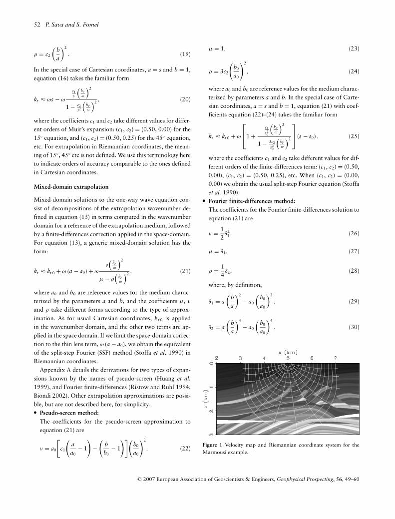
Figure 1 Velocity map and Riemannian coordinate system for theMarmousi example.



(a) (b)

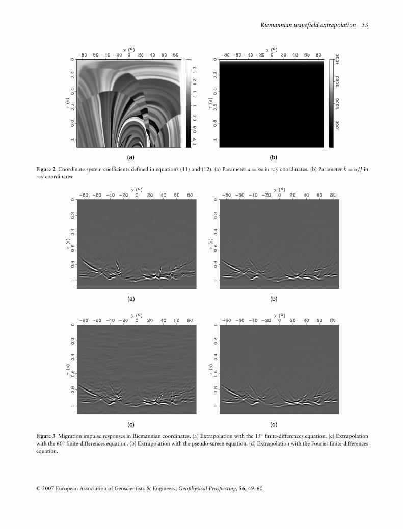
Figure 2 Coordinate system coefficients defined in equations (11) and (12). (a) Parameter a = sα in ray coordinates. (b) Parameter b = α/J inray coordinates.

(a) (b)

(c) (d)

Figure 3 Migration impulse responses in Riemannian coordinates. (a) Extrapolation with the 15◦ finite-differences equation. (c) Extrapolationwith the 60◦ finite-differences equation. (b) Extrapolation with the pseudo-screen equation. (d) Extrapolation with the Fourier finite-differencesequation.



(a) (b)

(c) (d)

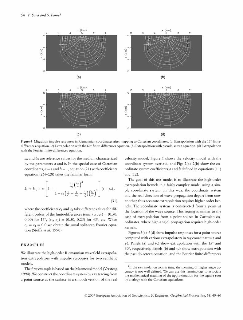
Figure 4 Migration impulse responses in Riemannian coordinates after mapping to Cartesian coordinates. (a) Extrapolation with the 15◦ finite-differences equation. (c) Extrapolation with the 60◦ finite-differences equation. (b) Extrapolation with pseudo-screen equation. (d) Extrapolationwith the Fourier finite-differences equation.

a0 and b0 are reference values for the medium characterizedby the parameters a and b. In the special case of Cartesiancoordinates, a = s and b = 1, equation (21) with coefficientsequation (26)–(28) takes the familiar form:

kτ ≈ kτ 0 + ω

⎡⎢⎣1 +

c1ss0

(kγ

ω

)2

1 − c2

(1s2 + 1

ss0+ 1

s20

)(kγ

ω

)2

⎤⎥⎦ (s − s0) ,

(31)

where the coefficients c1 and c2 take different values for dif-ferent orders of the finite-differences term: (c1, c2) = (0.50,0.00) for 15◦, (c1, c2) = (0.50, 0.25) for 45◦, etc. Whenc1 = c2 = 0.0 we obtain the usual split-step Fourier equa-tion (Stoffa et al. 1990).

E X A M P L E S

We illustrate the high-order Riemannian wavefield extrapola-tion extrapolators with impulse responses for two syntheticmodels.

The first example is based on the Marmousi model (Versteeg1994). We construct the coordinate system by ray tracing froma point source at the surface in a smooth version of the real

velocity model. Figure 1 shows the velocity model with thecoordinate system overlaid, and Figs 2(a)–2(b) show the co-ordinate system coefficients a and b defined in equations (11)and (12).

The goal of this test model is to illustrate the high-orderextrapolation kernels in a fairly complex model using a sim-ple coordinate system. In this way, the coordinate systemand the real direction of wave propagation depart from one-another, thus accurate extrapolation requires higher order ker-nels. The coordinate system is constructed from a point atthe location of the wave source. This setting is similar to thecase of extrapolation from a point source in Cartesian co-ordinates, where high-angle1 propagation requires high-orderkernels.

Figures 3(a)–3(d) show impulse responses for a point sourcecomputed with various extrapolators in ray coordinates (τ andγ ). Panels (a) and (c) show extrapolation with the 15◦ and60◦, respectively. Panels (b) and (d) show extrapolation withthe pseudo-screen equation, and the Fourier finite-differences

1If the extrapolation axis is time, the meaning of higher angle ac-curacy is not well defined. We can use this terminology to associatethe mathematical meaning of the approximation for the square-rootby analogy with the Cartesian equivalents.



(a)

(b)

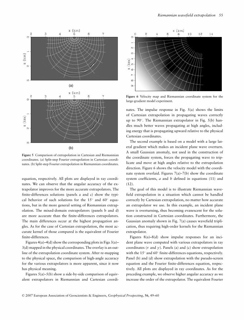
Figure 5 Comparison of extrapolation in Cartesian and Riemanniancoordinates. (a) Split-step Fourier extrapolation in Cartesian coordi-nates. (b) Split-step Fourier extrapolation in Riemannian coordinates.

equation, respectively. All plots are displayed in ray coordi-nates. We can observe that the angular accuracy of the ex-trapolator improves for the more accurate extrapolators. Thefinite-differences solutions (panels a and c) show the typi-cal behavior of such solutions for the 15◦ and 60◦ equa-tions, but in the more general setting of Riemannian extrap-olation. The mixed-domain extrapolators (panels b and d)are more accurate than the finite-differences extrapolators.The main differences occur at the highest propagation an-gles. As for the case of Cartesian extrapolation, the most ac-curate kernel of those compared is the equivalent of Fourierfinite-differences.

Figures 4(a)–4(d) show the corresponding plots in Figs 3(a)–3(d) mapped in the physical coordinates. The overlay is an out-line of the extrapolation coordinate system. After re-mappingto the physical space, the comparison of high-angle accuracyfor the various extrapolators is more apparent, since it nowhas physical meaning.

Figures 5(a)–5(b) show a side-by-side comparison of equiv-alent extrapolators in Riemannian and Cartesian coordi-

Figure 6 Velocity map and Riemannian coordinate system for thelarge-gradient model experiment.

nates. The impulse response in Fig. 5(a) shows the limitsof Cartesian extrapolation in propagating waves correctlyup to 90◦. The Riemannian extrapolator in Fig. 5(b) han-dles much better waves propagating at high angles, includ-ing energy that is propagating upward relative to the physicalCartesian coordinates.

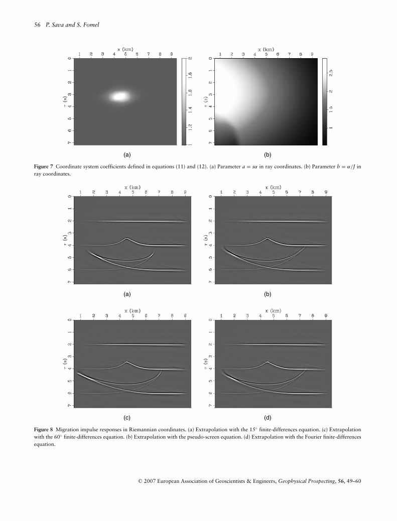
The second example is based on a model with a large lat-eral gradient which makes an incident plane wave overturn.A small Gaussian anomaly, not used in the construction ofthe coordinate system, forces the propagating wave to trip-licate and move at high angles relative to the extrapolationdirection. Figure 6 shows the velocity model with the coordi-nate system overlaid. Figures 7(a)–7(b) show the coordinatesystem coefficients, a and b defined in equations (11) and(12).

The goal of this model is to illustrate Riemannian wave-field extrapolation in a situation which cannot be handledcorrectly by Cartesian extrapolation, no matter how accuratean extrapolator we use. In this example, an incident planewave is overturning, thus becoming evanescent for the solu-tion constructed in Cartesian coordinates. Furthermore, theGaussian anomaly shown in Fig. 7(a) causes wavefield tripli-cation, thus requiring high-order kernels for the Riemannianextrapolator.

Figures 8(a)–8(d) show impulse responses for an inci-dent plane wave computed with various extrapolators in raycoordinates (τ and γ ). Panels (a) and (c) show extrapolationwith the 15◦ and 60◦ finite-differences equations, respectively.Panel (b) and (d) show extrapolation with the pseudo-screenequation and the Fourier finite-differences equation, respec-tively. All plots are displayed in ray coordinates. As for thepreceding example, we observe higher angular accuracy as weincrease the order of the extrapolator. The equivalent Fourier



(a) (b)

Figure 7 Coordinate system coefficients defined in equations (11) and (12). (a) Parameter a = sα in ray coordinates. (b) Parameter b = α/J inray coordinates.

(a) (b)

(c) (d)

Figure 8 Migration impulse responses in Riemannian coordinates. (a) Extrapolation with the 15◦ finite-differences equation. (c) Extrapolationwith the 60◦ finite-differences equation. (b) Extrapolation with the pseudo-screen equation. (d) Extrapolation with the Fourier finite-differencesequation.



(a) (b)

(c) (d)

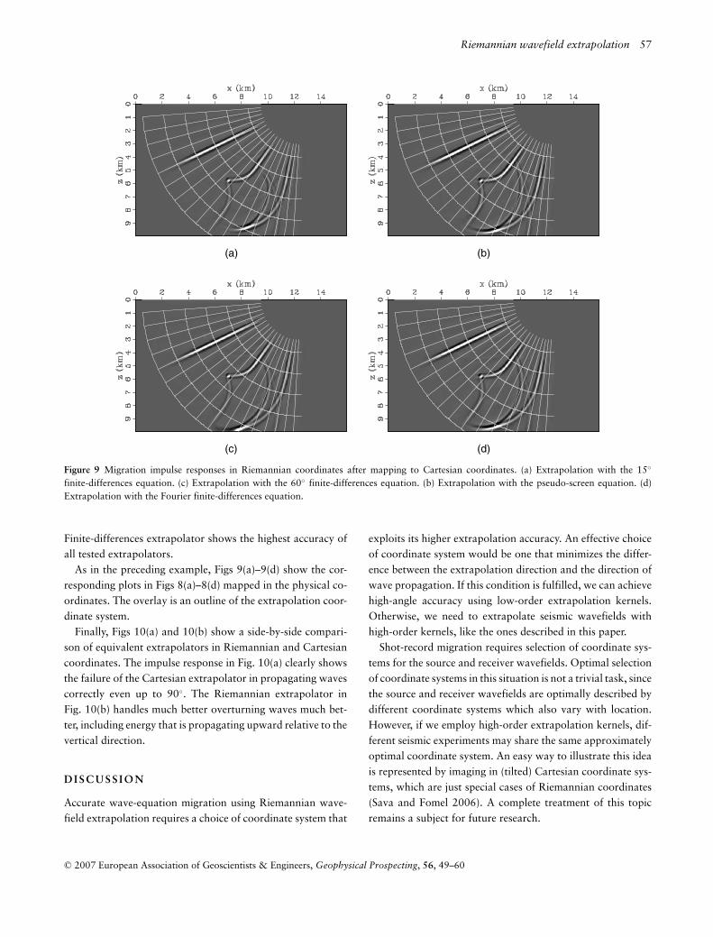
Figure 9 Migration impulse responses in Riemannian coordinates after mapping to Cartesian coordinates. (a) Extrapolation with the 15◦

finite-differences equation. (c) Extrapolation with the 60◦ finite-differences equation. (b) Extrapolation with the pseudo-screen equation. (d)Extrapolation with the Fourier finite-differences equation.

Finite-differences extrapolator shows the highest accuracy ofall tested extrapolators.

As in the preceding example, Figs 9(a)–9(d) show the cor-responding plots in Figs 8(a)–8(d) mapped in the physical co-ordinates. The overlay is an outline of the extrapolation coor-dinate system.

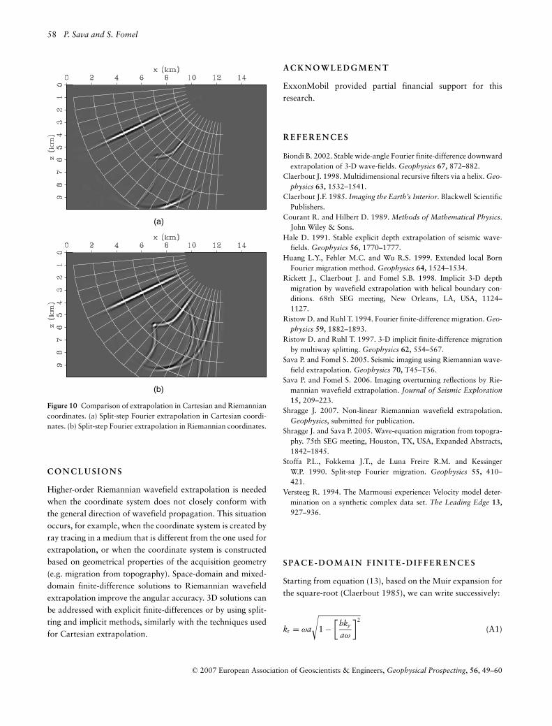
Finally, Figs 10(a) and 10(b) show a side-by-side compari-son of equivalent extrapolators in Riemannian and Cartesiancoordinates. The impulse response in Fig. 10(a) clearly showsthe failure of the Cartesian extrapolator in propagating wavescorrectly even up to 90◦. The Riemannian extrapolator inFig. 10(b) handles much better overturning waves much bet-ter, including energy that is propagating upward relative to thevertical direction.

D I S C U S S I O N

Accurate wave-equation migration using Riemannian wave-field extrapolation requires a choice of coordinate system that

exploits its higher extrapolation accuracy. An effective choiceof coordinate system would be one that minimizes the differ-ence between the extrapolation direction and the direction ofwave propagation. If this condition is fulfilled, we can achievehigh-angle accuracy using low-order extrapolation kernels.Otherwise, we need to extrapolate seismic wavefields withhigh-order kernels, like the ones described in this paper.

Shot-record migration requires selection of coordinate sys-tems for the source and receiver wavefields. Optimal selectionof coordinate systems in this situation is not a trivial task, sincethe source and receiver wavefields are optimally described bydifferent coordinate systems which also vary with location.However, if we employ high-order extrapolation kernels, dif-ferent seismic experiments may share the same approximatelyoptimal coordinate system. An easy way to illustrate this ideais represented by imaging in (tilted) Cartesian coordinate sys-tems, which are just special cases of Riemannian coordinates(Sava and Fomel 2006). A complete treatment of this topicremains a subject for future research.



(a)

(b)

Figure 10 Comparison of extrapolation in Cartesian and Riemanniancoordinates. (a) Split-step Fourier extrapolation in Cartesian coordi-nates. (b) Split-step Fourier extrapolation in Riemannian coordinates.

C O N C L U S I O N S

Higher-order Riemannian wavefield extrapolation is neededwhen the coordinate system does not closely conform withthe general direction of wavefield propagation. This situationoccurs, for example, when the coordinate system is created byray tracing in a medium that is different from the one used forextrapolation, or when the coordinate system is constructedbased on geometrical properties of the acquisition geometry(e.g. migration from topography). Space-domain and mixed-domain finite-difference solutions to Riemannian wavefieldextrapolation improve the angular accuracy. 3D solutions canbe addressed with explicit finite-differences or by using split-ting and implicit methods, similarly with the techniques usedfor Cartesian extrapolation.

A C K N O W L E D G M E N T

ExxonMobil provided partial financial support for thisresearch.

R E F E R E N C E S

Biondi B. 2002. Stable wide-angle Fourier finite-difference downwardextrapolation of 3-D wave-fields. Geophysics 67, 872–882.

Claerbout J. 1998. Multidimensional recursive filters via a helix. Geo-physics 63, 1532–1541.

Claerbout J.F. 1985. Imaging the Earth’s Interior. Blackwell ScientificPublishers.

Courant R. and Hilbert D. 1989. Methods of Mathematical Physics.John Wiley & Sons.

Hale D. 1991. Stable explicit depth extrapolation of seismic wave-fields. Geophysics 56, 1770–1777.

Huang L.Y., Fehler M.C. and Wu R.S. 1999. Extended local BornFourier migration method. Geophysics 64, 1524–1534.

Rickett J., Claerbout J. and Fomel S.B. 1998. Implicit 3-D depthmigration by wavefield extrapolation with helical boundary con-ditions. 68th SEG meeting, New Orleans, LA, USA, 1124–1127.

Ristow D. and Ruhl T. 1994. Fourier finite-difference migration. Geo-physics 59, 1882–1893.

Ristow D. and Ruhl T. 1997. 3-D implicit finite-difference migrationby multiway splitting. Geophysics 62, 554–567.

Sava P. and Fomel S. 2005. Seismic imaging using Riemannian wave-field extrapolation. Geophysics 70, T45–T56.

Sava P. and Fomel S. 2006. Imaging overturning reflections by Rie-mannian wavefield extrapolation. Journal of Seismic Exploration15, 209–223.

Shragge J. 2007. Non-linear Riemannian wavefield extrapolation.Geophysics, submitted for publication.

Shragge J. and Sava P. 2005. Wave-equation migration from topogra-phy. 75th SEG meeting, Houston, TX, USA, Expanded Abstracts,1842–1845.

Stoffa P.L., Fokkema J.T., de Luna Freire R.M. and KessingerW.P. 1990. Split-step Fourier migration. Geophysics 55, 410–421.

Versteeg R. 1994. The Marmousi experience: Velocity model deter-mination on a synthetic complex data set. The Leading Edge 13,927–936.

S PA C E - D O M A I N F I N I T E - D I F F E R E N C E S

Starting from equation (13), based on the Muir expansion forthe square-root (Claerbout 1985), we can write successively:

kτ = ωa

√1 −

[bkγ

aω

]2

(A1)



≈ ωa

⎡⎢⎣1 −

c1

[bkγ

aω

]2

1 − c2

[bkγ

aω

]2

⎤⎥⎦ (A2)

≈ ωa − ωc1a

(ba

)2(

kγ

ω

)2

1 − c2(

ba

)2(

kγ

ω

)2 . (A3)

If we make the notations

ν = −c1a(

ba

)2

, (A4)

μ = 1, (A5)

ρ = c2

(ba

)2

. (A6)

we obtain the finite-differences solution to the one-way waveequation in Riemannian coordinates:

kτ ≈ ωa + ων

(kγ

ω

)2

μ − ρ(

kγ

ω

)2 . (A7)

M I X E D D O M A I N — P S E U D O - S C R E E N

The pseudo-screen solution to equation (13) derives from afirst-order expansion of the square-root around a0 and b0

which are reference values for the medium characterized bythe parameters a and b:

kτ ≈ kτ 0 + ∂kτ

∂a

∣∣∣∣a0,b0

(a − a0) + ∂kτ

∂b

∣∣∣∣a0,b0

(b − b0) . (A8)

The partial derivatives relative to a and b, respectively, are:

∂kτ

∂a

∣∣∣∣a0,b0

= ω1√

1 −(

b0kγ

a0ω

)2≈ ω

⎡⎢⎣1 +

c1

(b0kγ

a0ω

)2

1 − 3c2

(b0kγ

a0ω

)2

⎤⎥⎦ ,

(A9)

∂kτ

∂b

∣∣∣∣a0,b0

= −ωb0

a0

(kγ

ω

)2 1√1 −

(b0kγ

a0ω

)2≈ −ω

a0

b0

(b0kγ

a0ω

)2

.

(A10)

Therefore, the pseudo-screen equation becomes

kτ ≈ kτ 0 + ω (a − a0)

+ωa0

[c1

(aa0

− 1)

−(

bb0

− 1)] (

b0a0

)2 (kγ

ω

)2

1 − 3c2

(b0a0

)2 (kγ

ω

)2 . (A11)


ν = a0

[c1

(aa0

− 1)

−(

bb0

− 1)] (

b0

a0

)2

(A12)

μ = 1 (A13)

ρ = 3c2

(b0

a0

)2

(A14)

we obtain the mixed-domain pseudo-screen solution to theone-way wave equation in Riemannian coordinates:

kτ ≈ kτ 0 + ω (a − a0) + ων

(kγ

ω

)2

μ − ρ(

kγ

ω

)2 . (A15)

M I X E D D O M A I N — F O U R I E RF I N I T E - D I F F E R E N C E S

The pseudo-screen solution to equation (13) derives from afourth-order expansion of the square-root around (a0, b0) and(a, b):

kτ ≈ ωa

[1 + 1

2

[bkγ

aω

]2

+ 18

(bkγ

aω

)4]

, (A16)

kτ 0 ≈ ωa0

[1 + 1

2

(b0kγ

a0ω

)2

+ 18

(b0kγ

a0ω

)4]

. (A17)

If we subtract equations (A16) and (A17), we obtain the fol-lowing expression for the wavenumber along the extrapola-tion direction kτ :

kτ ≈ kτ 0 + ω(a − a0) + 12

ω

[a

(ba

)2

− a0

(b0

a0

)2](kγ

ω

)2

+18

ω

[a

(ba

)4

− a0

(b0

a0

)4](kγ

ω

)4

. (A18)

We can make the notations

δ1 = a

(ba

)2

− a0

(b0

a0

)2

, (A19)

δ2 = a

(ba

)4

− a0

(b0

a0

)4

, (A20)

therefore equation (A18) can be written as

kτ = kτ 0 + ω(a − a0) + 12

ωδ1

(kγ

ω

)2

+ 18

ωδ2

(kγ

ω

)4

. (A21)



Using the approximation

12

δ1u2 + 18

δ2u4 ≈12 δ2

1u2

δ1 − 14 δ2u2

, (A22)

we can write

kτ = kτ 0 + ω(a − a0) + ω

12 δ2

1

(kγ

ω

)2

δ1 − 14 δ2

(kγ

ω

)2 . (A23)


ν = 12

δ21, (A24)

μ = δ1, (A25)

ρ = 14

δ2, (A26)

we obtain the mixed-domain Fourier finite-differences so-lution to the one-way wave equation in Riemanniancoordinates:

kτ ≈ kτ 0 + ω(a − a0) + ων

(kγ

ω

)2

μ − ρ(

kγ

ω

)2 . (A27)


High-order kernels for Riemannian wavefield … P. Sava and S. Fomel ρ = c 2 b a 2. (19) In the...

Documents

Transcript of High-order kernels for Riemannian wavefield … P. Sava and S. Fomel ρ = c 2 b a 2. (19) In the...