Heterogeneous firms and aggregate TFP - Paul Klein

Heterogeneous firms and aggregate TFP

Question: how important are firm-specific distortions fordevelopment (output per worker differences)?

Rogerson and Restuccia (2008)

Hsieh and Klenow (2009)

Guner, Ventura and Xu (2008)

Guner, Ventura and Parkhomenko (2015)

P. Klein Heterogeneous firms and aggregate TFP 1 / 28

Rogerson & Restuccia (2008)

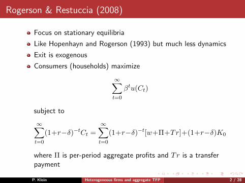
Focus on stationary equilibria

Like Hopenhayn and Rogerson (1993) but much less dynamics

Exit is exogenous

Consumers (households) maximize

∞∑t=0

βtu(Ct)

subject to

∞∑t=0

(1+r−δ)−tCt =

∞∑t=0

(1+r−δ)−t[w+Π+Tr]+(1+r−δ)K0

where Π is per-period aggregate profits and Tr is a transferpayment



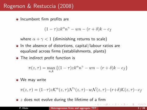
Incumbent firm profits are

(1− τ)zkαnγ − wn− (r + δ)k − cf

where α+ γ < 1 (diminishing returns to scale)

In the absence of distortions, capital/labour ratios areequalized across firms (establishments, plants)

The indirect profit function is

π(z, τ) = maxn,k{(1− τ)zkαnγ − wn− (r + δ)k − cf}

We may write

π(z, τ) = (1−τ)zKα(z, τ)N γ(z, τ)−wN (z, τ)−(r+δ)K(z, τ)−cf

z does not evolve during the lifetime of a firm



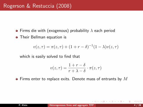
Firms die with (exogenous) probability λ each period

Their Bellman equation is

v(z, τ) = π(z, τ) + (1 + r − δ)−1(1− λ)v(z, τ)

which is easily solved to find that

v(z, τ) =1 + r − δr + λ− δ

· π(z, τ)

Firms enter to replace exits. Denote mass of entrants by M



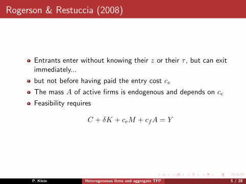
Entrants enter without knowing their z or their τ , but can exitimmediately...

but not before having paid the entry cost ce

The mass A of active firms is endogenous and depends on ce

Feasibility requires

C + δK + ceM + cfA = Y



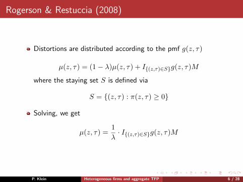
Distortions are distributed according to the pmf g(z, τ)

µ(z, τ) = (1− λ)µ(z, τ) + I{(z,τ)∈S}g(z, τ)M

where the staying set S is defined via

S = {(z, τ) : π(z, τ) ≥ 0}

Solving, we get

µ(z, τ) =1

λ· I{(z,τ)∈S}g(z, τ)M



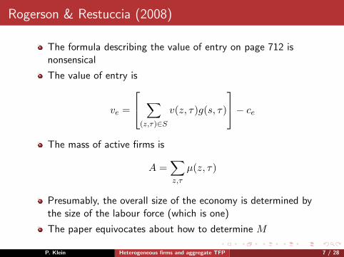
The formula describing the value of entry on page 712 isnonsensical

The value of entry is

ve =

∑(z,τ)∈S

v(z, τ)g(s, τ)

− ceThe mass of active firms is

A =∑z,τ

µ(z, τ)

Presumably, the overall size of the economy is determined bythe size of the labour force (which is one)

The paper equivocates about how to determine M



Definition of a stationary equilibrium

Constituents of an equilibrium

µwrTrMv(z, τ)π(z, τ)veSN (z, τ)K(z, τ)CKΠ



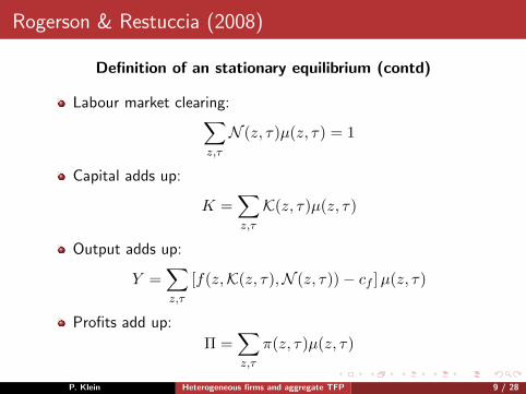
Definition of an stationary equilibrium (contd)

Labour market clearing:∑z,τ

N (z, τ)µ(z, τ) = 1

Capital adds up:

K =∑z,τ

K(z, τ)µ(z, τ)

Output adds up:

Y =∑z,τ

[f(z,K(z, τ),N (z, τ))− cf ]µ(z, τ)

Profits add up:

Π =∑z,τ

π(z, τ)µ(z, τ)



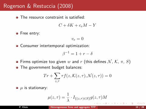
The resource constraint is satisfied:

C + δK + ceM − Y

Free entry:ve = 0

Consumer intertemporal optimization:

β−1 = 1 + r − δ

Firms optimize too given w and r (this defines N , K, π, S)

The government budget balances:

Tr +∑z,τ

τf(z,K(z, τ),N (z, τ)) = 0

µ is stationary:

µ(z, τ) =1

λ· I{(z,τ)∈S}g(z, τ)M



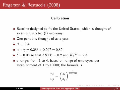
Calibration

Baseline designed to fit the United States, which is thought ofas an undistorted (!) economy

One period is thought of as a year

β = 0.96

α+ γ = 0.283 + 0.567 = 0.85

δ = 0.08 so that δK/Y = 0.2 and K/Y = 2.3

z ranges from 1 to 4, based on range of employees perestablishment of 1 to 10000; the formula is

ninj

=

(zizj

) 11−γ−α



Calibration contd

cf = 0 (all firms that enter operate)

ce = 1 (a normalization; changing it is like scaling TFP)

The distribution h of z is (non-parametrically) such as toreplicate the size (employment) distribution across firms(establishments)

λ = .1



Size distribution of establishments

1-5 5-49 50+

Model .56 .39 .05Data .56 .39 .05



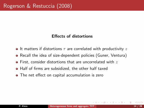
Effects of distortions

It matters if distortions τ are correlated with productivity z

Recall the idea of size-dependent policies (Guner, Ventura)

First, consider distortions that are uncorrelated with z

Half of firms are subsidized, the other half taxed

The net effect on capital accumulation is zero



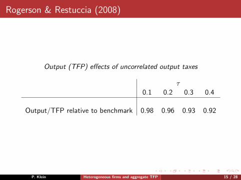
Output (TFP) effects of uncorrelated output taxes

τ0.1 0.2 0.3 0.4

Output/TFP relative to benchmark 0.98 0.96 0.93 0.92



Effects of correlated distortions

Below median productivity firms receive a subsidy

Above median productivity firms pay a tax

Output (TFP) effects of correlated distortions

τ0.1 0.2 0.3 0.4

Output/TFP relative to benchmark 0.90 0.80 0.73 0.69



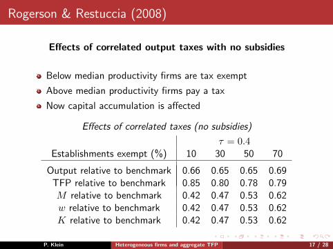
Effects of correlated output taxes with no subsidies

Below median productivity firms are tax exempt

Above median productivity firms pay a tax

Now capital accumulation is affected

Effects of correlated taxes (no subsidies)

τ = 0.4Establishments exempt (%) 10 30 50 70

Output relative to benchmark 0.66 0.65 0.65 0.69TFP relative to benchmark 0.85 0.80 0.78 0.79M relative to benchmark 0.42 0.47 0.53 0.62w relative to benchmark 0.42 0.47 0.53 0.62K relative to benchmark 0.42 0.47 0.53 0.62


Hsieh & Klenow (2009)

Question: how important is misallocation of resources acrossfirms in China and India for their level of development?

Specifically, how much would GDP per worker rise in thesecountries if resources were reallocated optimally across firms?

Lots of analytical formulas—hence the publication in QJE

Big contribution: measuring firm-level TFP in China and Indialeading to a tighter connection with data—hence the manycitations



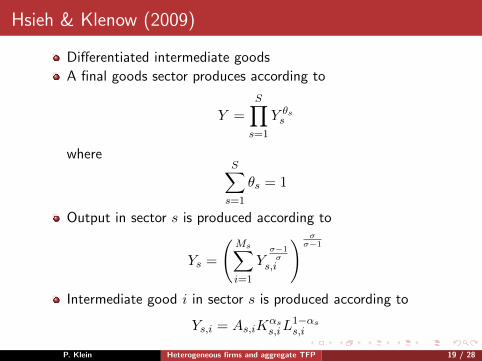
Differentiated intermediate goods

A final goods sector produces according to

Y =

S∏s=1

Y θss

whereS∑s=1

θs = 1

Output in sector s is produced according to

Ys =

(Ms∑i=1

Yσ−1σ

s,i

) σσ−1

Intermediate good i in sector s is produced according to

Ys,i = As,iKαss,iL

1−αss,i



Firm profits are given by

πs,i = (1− τY,s,i)Ps,iYs,i − wLs,i − (1 + τK,s,i)RKs,i

No labour distortion

Explicit expressions for

Firm level Price Ps,iFirm level MRPLs,iFirm level MRPKs,i

Sectoral labour LsSectoral capital Ks

Sectoral TFPs



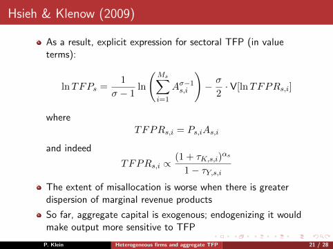
As a result, explicit expression for sectoral TFP (in valueterms):

lnTFPs =1

σ − 1ln

(Ms∑i=1

Aσ−1s,i

)− σ

2· V[lnTFPRs,i]

whereTFPRs,i = Ps,iAs,i

and indeed

TFPRs,i ∝(1 + τK,s,i)

αs

1− τY,s,iThe extent of misallocation is worse when there is greaterdispersion of marginal revenue products

So far, aggregate capital is exogenous; endogenizing it wouldmake output more sensitive to TFP



Data

Firm level data on

Value addedCapital stock (book value)Wage payments



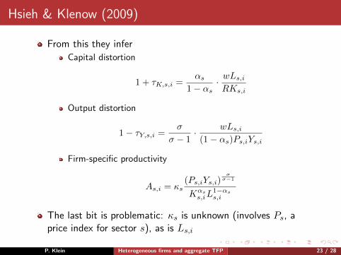
From this they infer

Capital distortion

1 + τK,s,i =αs

1− αs· wLs,iRKs,i

Output distortion

1− τY,s,i =σ

σ − 1· wLs,i

(1− αs)Ps,iYs,i

Firm-specific productivity

As,i = κs(Ps,iYs,i)

σσ−1

Kαss,iL

1−αss,i

The last bit is problematic: κs is unknown (involves Ps, aprice index for sector s), as is Ls,i



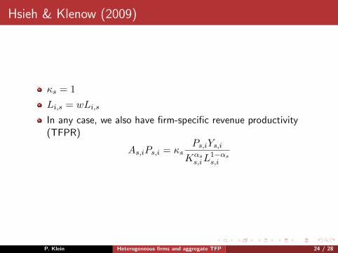
κs = 1

Li,s = wLi,s

In any case, we also have firm-specific revenue productivity(TFPR)

As,iPs,i = κsPs,iYs,i

Kαss,iL

1−αss,i



Calibration

σ = 3

R = 0.1

αs equal to whatever it is in the U.S. manufacturing industry



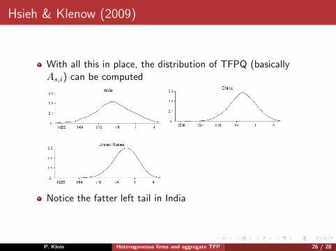
With all this in place, the distribution of TFPQ (basicallyAs,i) can be computed

Notice the fatter left tail in India



Meanwhile, here is the distribution of TFPR:

Notice the bigger dispersion in India and China



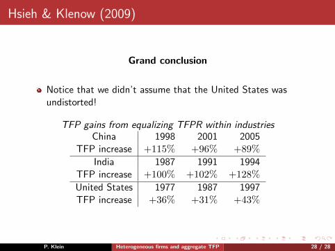
Grand conclusion

Notice that we didn’t assume that the United States wasundistorted!

TFP gains from equalizing TFPR within industriesChina 1998 2001 2005

TFP increase +115% +96% +89%

India 1987 1991 1994TFP increase +100% +102% +128%

United States 1977 1987 1997TFP increase +36% +31% +43%


Heterogeneous firms and aggregate TFP - Paul Klein

Documents

Transcript of Heterogeneous firms and aggregate TFP - Paul Klein