Aggregate Recruiting Intensity - New York University is aggregate recruiting intensity? ... Bersin...
52
Aggregate Recruiting Intensity Alessandro Gavazza London School of Economics Simon Mongey New York University Gianluca Violante New York University OSU - August 23, 2016
Transcript of Aggregate Recruiting Intensity - New York University is aggregate recruiting intensity? ... Bersin...
yl
Aggregate Recruiting Intensity
Alessandro GavazzaLondon School of Economics
Simon MongeyNew York University
Gianluca ViolanteNew York University
OSU - August 23, 2016
Introductionyyl
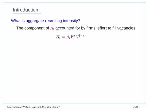
What is aggregate recruiting intensity?
The component of At accounted for by firms’ effort to fill vacancies
Ht = AtVαt U1−α
t
Gavazza-Mongey-Violante, "Aggregate Recruiting Intensity" p.1/33hello
Introductionyyl
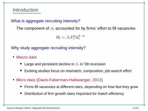
What is aggregate recruiting intensity?
The component of At accounted for by firms’ effort to fill vacancies
Ht = AtVαt U1−α
t
Why study aggregate recruiting intensity?
• Macro data
Large and persistent decline in At in ‘08 recession
Existing studies focus on mismatch, composition, job-search effort
• Micro data (Davis-Faberman-Haltiwanger, 2013)
Firms fill vacancies at different rates, depending on how fast they grow
Distribution of firm growth rates important for match efficiency
Gavazza-Mongey-Violante, "Aggregate Recruiting Intensity" p.1/33hello
Introductionyyl
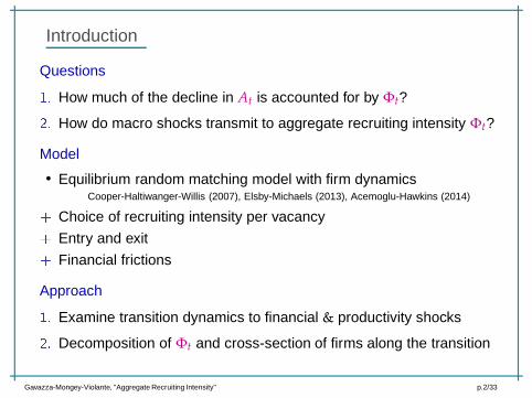
Questions
1. How much of the decline in At is accounted for by Φt?
2. How do macro shocks transmit to aggregate recruiting intensity Φt?
Model
• Equilibrium random matching model with firm dynamicsCooper-Haltiwanger-Willis (2007), Elsby-Michaels (2013), Acemoglu-Hawkins (2014)
+ Choice of recruiting intensity per vacancy
+ Entry and exit
+ Financial frictions
Approach
1. Examine transition dynamics to financial & productivity shocks
2. Decomposition of Φt and cross-section of firms along the transition
Gavazza-Mongey-Violante, "Aggregate Recruiting Intensity" p.2/33hello
Firm-level hiring technologyyl
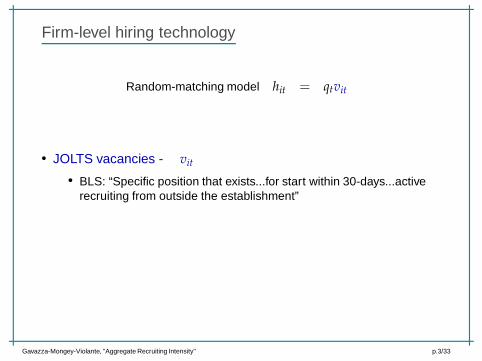
Random-matching model hit = qtvit
+ recruiting effort hit = qteitvit
• JOLTS vacancies - vit
• BLS: “Specific position that exists...for start within 30-days...activerecruiting from outside the establishment”
Gavazza-Mongey-Violante, "Aggregate Recruiting Intensity" p.3/33hello
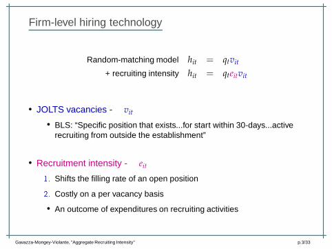
Firm-level hiring technologyyl
Random-matching model hit = qtvit
+ recruiting intensity hit = qteitvit
• JOLTS vacancies - vit
• BLS: “Specific position that exists...for start within 30-days...activerecruiting from outside the establishment”
• Recruitment intensity - eit
1. Shifts the filling rate of an open position
2. Costly on a per vacancy basis
• An outcome of expenditures on recruiting activities
Gavazza-Mongey-Violante, "Aggregate Recruiting Intensity" p.3/33hello
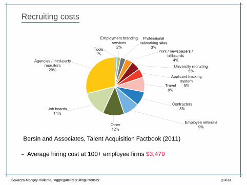
Recruiting costsy
Tools 1%
Employment branding services
2%
Professional networking sites
3% Print / newspapers /
billboards 4%
University recruiting 5%
Applicant tracking system
5% Travel 8%
Contractors 8%
Employee referrals 9%
Other 12%
Job boards 14%
Agencies / third-party recruiters
29%
Bersin and Associates, Talent Acquisition Factbook (2011)
- Average hiring cost at 100+ employee firms $3,479
Gavazza-Mongey-Violante, "Aggregate Recruiting Intensity" p.4/33hello
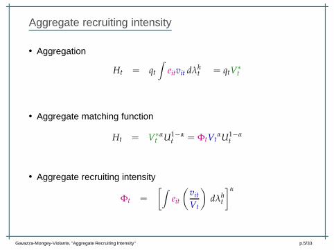
Aggregate recruiting intensityyl
• Aggregation
Ht = qt
∫
eitvit dλht = qtV
∗t
• Aggregate matching function
Ht = V∗t
αU1−αt = ΦtVt
αU1−αt
• Aggregate recruiting intensity
Φt =
[∫
eit
(vit
Vt
)
dλht
]α
Gavazza-Mongey-Violante, "Aggregate Recruiting Intensity" p.5/33hello
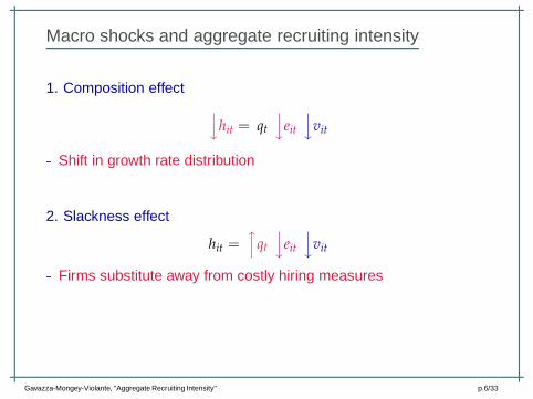
Macro shocks and aggregate recruiting intensityyl
1. Composition effectyhit = qt
yeit
yvit
- Shift in growth rate distribution
2. Slackness effect
hit =xqt
yeit
yvit
- Firms substitute away from costly hiring measures
Gavazza-Mongey-Violante, "Aggregate Recruiting Intensity" p.6/33hello
Value functionsyyl
Gavazza-Mongey-Violante, "Aggregate Recruiting Intensity" p.7/33hello
Value functionsyyl
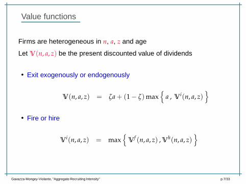
Firms are heterogeneous in n, a, z and age
Let V(n, a, z) be the present discounted value of dividends
• Exit exogenously or endogenously
V(n, a, z) = ζa + (1 − ζ)max
a , Vi(n, a, z)
• Fire or hire
Vi(n, a, z) = max
Vf (n, a, z) , V
h(n, a, z)
Gavazza-Mongey-Violante, "Aggregate Recruiting Intensity" p.7/33hello
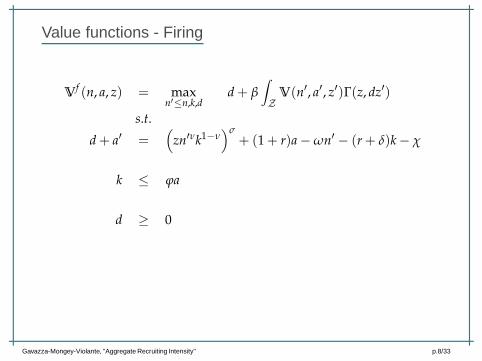
Value functions - Firingyl
Vf (n, a, z) = max
n′≤n,k,dd + β
∫
ZV(n′, a′, z′)Γ(z, dz′)
s.t.
d + a′ =(
zn′νk1−ν)σ
+ (1 + r)a − ωn′ − (r + δ)k − χ
k ≤ ϕa
d ≥ 0
Gavazza-Mongey-Violante, "Aggregate Recruiting Intensity" p.8/33hello
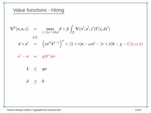
Value functions - Hiringyl
Vh(n, a, z) = max
v>0,e>0,k,dd + β
∫
ZV(n′, a′, z′)Γ(z, dz′)
s.t.
d + a′ =(
zn′νk1−ν)σ
+ (1 + r)a − ωn′ − (r + δ)k − χ − C(e, v, n)
n′ − n = q(θ∗)ev
k ≤ ϕa
d ≥ 0
Gavazza-Mongey-Violante, "Aggregate Recruiting Intensity" p.9/33hello
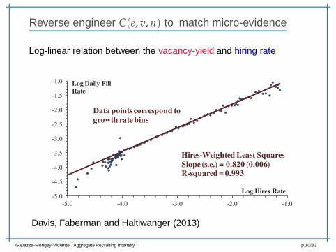
Reverse engineer C(e, v, n) toymatch micro-evidencey
Log-linear relation between the vacancy-yield and hiring rate
-5.0
-4.5
-4.0
-3.5
-3.0
-2.5
-2.0
-1.5
-1.0
-5.0 -4.0 -3.0 -2.0 -1.0
Log Daily Fill Rate
Log Hires Rate
Hires-Weighted Least Squares
Slope (s.e.) = 0.820 (0.006)R-squared = 0.993
Data points correspond to
growth rate bins
Davis, Faberman and Haltiwanger (2013)
Gavazza-Mongey-Violante, "Aggregate Recruiting Intensity" p.10/33hello
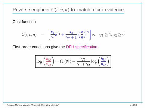
Reverse engineer C(e, v, n) toymatch micro-evidencey
Cost function
C(e, v, n) =
[κ1
γ1eγ1 +
κ2
γ2 + 1
(v
n
)γ2]
v, γ1 ≥ 1, γ2 ≥ 0
First-order conditions give the DFH specification
log
(hi,t
vi,t
)
= Ω (θ∗t ) +γ2
γ1 + γ2log
(hi,t
ni,t
)
Gavazza-Mongey-Violante, "Aggregate Recruiting Intensity" p.11/33hello
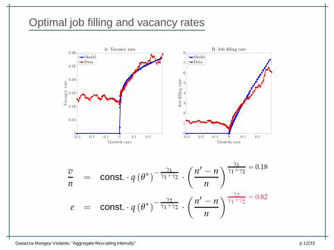
Optimal job filling and vacancy ratesyl
-0.3 -0.2 -0.1 0 0.1 0.2
Growth rate
0
0.01
0.02
0.03
0.04
0.05
0.06
Vacancy
rate
A. Vacancy rate
ModelData
-0.3 -0.2 -0.1 0 0.1 0.2
Growth rate
0
1
2
3
4
5
6
7
8
Jobfillingrate
B. Job filling rate
ModelData
v
n= const. · q (θ∗)
−γ1
γ1+γ2 ·
(n′ − n
n
) γ1γ1+γ2
= 0.18
e = const. · q (θ∗)−
γ2γ1+γ2 ·
(n′ − n
n
) γ2γ1+γ2
= 0.82
Gavazza-Mongey-Violante, "Aggregate Recruiting Intensity" p.12/33hello
Value functions - Entryyl
• Initial wealth Household allocates a0 to λ0 potential entrants
• Productivity Potential entrants draw z ∼ Γ0(z)
• Entry Choice to become incumbent and pay χ0 start-up costs
Ve(a0, z) = max
a0 , Vi (n0, a0 − χ0, z)
Selection at entry based only on productivity z
Given z, growth determined by financial constraints and hiring costs
Gavazza-Mongey-Violante, "Aggregate Recruiting Intensity" p.13/33hello
Equilibriumyl
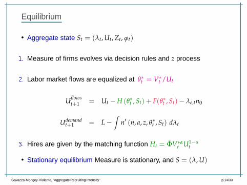
• Aggregate state St = (λt, Ut, Zt, ϕt)
1. Measure of firms evolves via decision rules and z process
2. Labor market flows are equalized at θ∗t = V∗t /Ut
Uflowst+1 = Ut − H (θ∗t , St) + F(θ∗t , St)− λe,tn0
Udemandt+1 = L −
∫
n′ (n, a, z, θ∗t , St) dλt
3. Hires are given by the matching function Ht = ΦV∗αt U1−α
t
• Stationary equilibrium Measure is stationary, and S = (λ, U)
Gavazza-Mongey-Violante, "Aggregate Recruiting Intensity" p.14/33hello
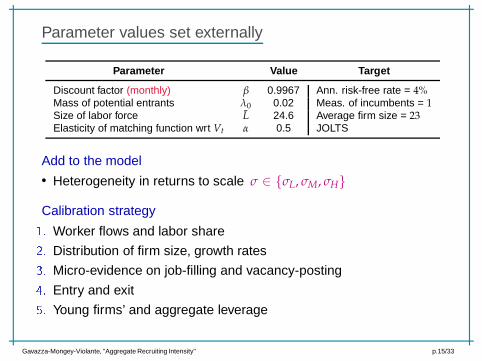
Parameter values set externallyyl
Parameter Value Target
Discount factor (monthly) β 0.9967 Ann. risk-free rate = 4%Mass of potential entrants λ0 0.02 Meas. of incumbents = 1Size of labor force L 24.6 Average firm size = 23Elasticity of matching function wrt Vt α 0.5 JOLTS
Add to the model• Heterogeneity in returns to scale σ ∈ σL, σM, σH
Calibration strategy
1. Worker flows and labor share
2. Distribution of firm size, growth rates
3. Micro-evidence on job-filling and vacancy-posting
4. Entry and exit
5. Young firms’ and aggregate leverage
Gavazza-Mongey-Violante, "Aggregate Recruiting Intensity" p.15/33hello
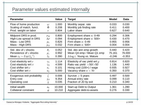
Parameter values estimated internallyyl
Parameter Value Target Model Data
Flow of home production ω 1.000 Monthly separ. rate 0.033 0.030Scaling of match. funct. Φ 0.208 Monthly job finding rate 0.411 0.400Prod. weight on labor ν 0.804 Labor share 0.627 0.640
Midpoint DRS in prod. σM 0.800 Employment share n: 0-49 0.294 0.306High-Low spread in DRS ∆σ 0.094 Employment share n: 500+ 0.430 0.470Mass - Low DRS µL 0.826 Firm share n: 0-49 0.955 0.956Mass - High DRS µH 0.032 Firm share n: 500+ 0.004 0.004
Std. dev of z shocks ϑz 0.052 Std. dev ann emp growth 0.440 0.420Persistence of z shocks ρz 0.992 Mean Q4 emp / Mean Q1 emp 75.161 76.000Mean z0 ∼ Exp(z−1
0 ) z0 0.390 ∆ log z: Young vs. Mature -0.246 -0.353
Cost elasticity wrt e γ1 1.114 Elasticity of vac yield wrt g 0.814 0.820Cost elasticity wrt v γ2 4.599 Ratio vac yield: <50/>50 1.136 1.440Cost shifter wrt e κ1 0.101 Hiring cost (100+) / wage 0.935 0.927Cost shifter wrt v κ2 5.000 Vacancy share n < 50 0.350 0.370
Exogenous exit probability ζ 0.006 Survive ≥ 5 years 0.497 0.500Entry cost χ0 9.354 Annual entry rate 0.099 0.110Operating cost χ 0.035 Fraction of JD by exit 0.210 0.340
Initial wealth a0 10.000 Start-up Debt to Output 1.361 1.280Collateral constraint ϕ 10.210 Aggregate debt-to-assets 0.276 0.330
Gavazza-Mongey-Violante, "Aggregate Recruiting Intensity" p.16/33hello
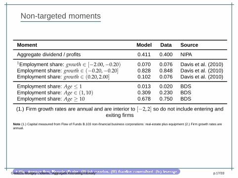
Non-targeted momentsyl
Moment Model Data Source
Aggregate dividend / profits 0.411 0.400 NIPA
1Employment share: growth ∈ [−2.00,−0.20) 0.070 0.076 Davis et al. (2010)Employment share: growth ∈ (−0.20,−0.20] 0.828 0.848 Davis et al. (2010)Employment share: growth ∈ (0.20, 2.00] 0.102 0.076 Davis et al. (2010)
Employment share: Age ≤ 1 0.013 0.020 BDSEmployment share: Age ∈ (1, 10) 0.309 0.230 BDSEmployment share: Age ≥ 10 0.678 0.750 BDS
(1.) Firm growth rates are annual and are interior to [−2, 2] so do not include entering andexiting firms
Note (1.) Capital measured from Flow of Funds B.103 non-financial business corporations: real-estate plus equipment (2.) Firm growth rates areannual.
Fig. Average rm life y le (i) size, (ii) job reation, (iii) fra tion onstrained, (iv) leverageGavazza-Mongey-Violante, "Aggregate Recruiting Intensity" p.17/33hello
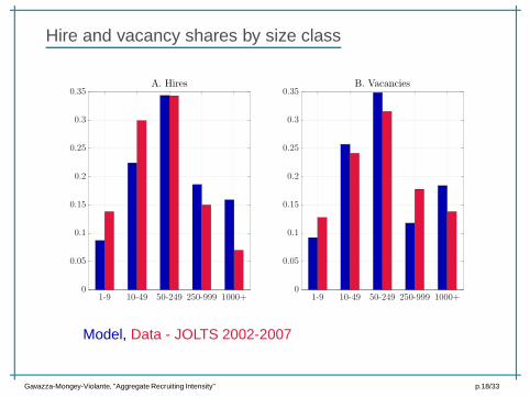
Hire and vacancy shares by size classyl
1-9 10-49 50-249 250-999 1000+0
0.05
0.1
0.15
0.2
0.25
0.3
0.35A. Hires
1-9 10-49 50-249 250-999 1000+0
0.05
0.1
0.15
0.2
0.25
0.3
0.35B. Vacancies
Model, Data - JOLTS 2002-2007
Gavazza-Mongey-Violante, "Aggregate Recruiting Intensity" p.18/33hello
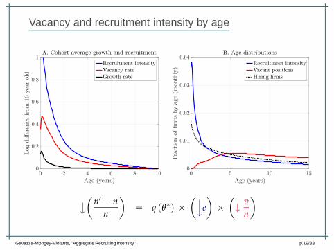
Vacancy and recruitment intensity by ageyl
0 2 4 6 8 10
Age (years)
0
0.2
0.4
0.6
0.8
1
Logdifferen
cefrom
10yearold
A. Cohort average growth and recruitment
Recruitment intensityVacancy rateGrowth rate
0 5 10 15
Age (years)
0
0.01
0.02
0.03
0.04
Fractionoffirm
sbyage(m
onthly)
B. Age distributions
Recruitment intensityVacant positionsHiring firms
y
(n′ − n
n
)
= q (θ∗) ×
(ye
)
×
(
↓v
n
)
Gavazza-Mongey-Violante, "Aggregate Recruiting Intensity" p.19/33hello
Transition dynamics experimentsyl
Gavazza-Mongey-Violante, "Aggregate Recruiting Intensity" p.20/33hello
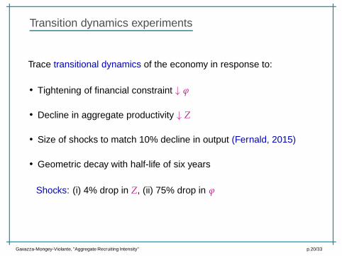
Transition dynamics experimentsyl
Trace transitional dynamics of the economy in response to:
• Tightening of financial constraint ↓ ϕ
• Decline in aggregate productivity ↓ Z
• Size of shocks to match 10% decline in output (Fernald, 2015)
• Geometric decay with half-life of six years
Shocks: (i) 4% drop in Z, (ii) 75% drop in ϕ
Gavazza-Mongey-Violante, "Aggregate Recruiting Intensity" p.20/33hello
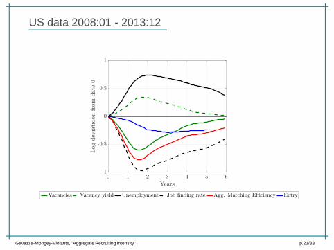
US data 2008:01 - 2013:12yyl
0 1 2 3 4 5 6
Years
-1
-0.5
0
0.5
1
Logdeviatioonfrom
date
0
Vacancies Vacancy yield Unemployment Job finding rate Agg. Matching Efficiency Entry
Gavazza-Mongey-Violante, "Aggregate Recruiting Intensity" p.21/33hello
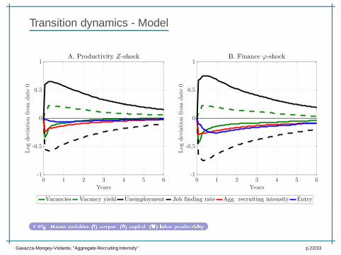
Transition dynamics - Modelyl
0 1 2 3 4 5 6Years
-1
-0.5
0
0.5
1
Logdeviationfrom
date
0
A. Productivity Z-shock
0 1 2 3 4 5 6Years
-1
-0.5
0
0.5
1
Logdeviationfrom
date
0
B. Finance ϕ-shock
Vacancies Vacancy yield Unemployment Job finding rate Agg. recruiting intensity Entry
Fig. Ma ro variables (i) output, (ii) apital, (iii) labor produ tivity
Gavazza-Mongey-Violante, "Aggregate Recruiting Intensity" p.22/33hello
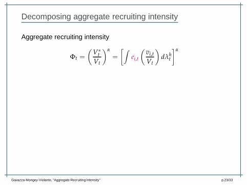
Decomposing aggregate recruiting intensityyl
Aggregate recruiting intensity
Φt =
(V∗
t
Vt
)α
=
[∫
ei,t
(vi,t
Vt
)
dλht
]α
Gavazza-Mongey-Violante, "Aggregate Recruiting Intensity" p.23/33hello
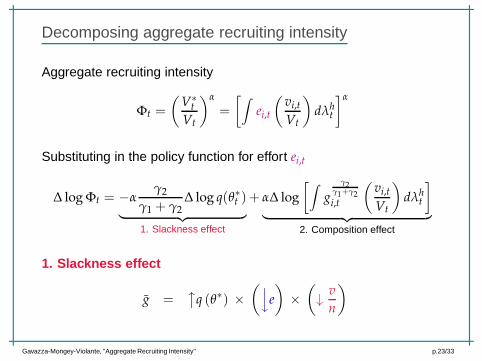
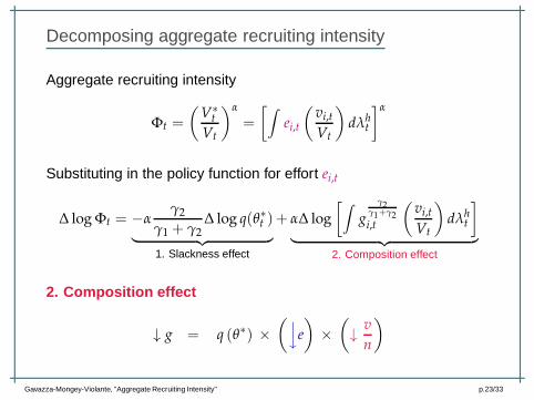
Decomposing aggregate recruiting intensityyl
Aggregate recruiting intensity
Φt =
(V∗
t
Vt
)α
=
[∫
ei,t
(vi,t
Vt
)
dλht
]α
Substituting in the policy function for effort ei,t
∆ log Φt = −αγ2
γ1 + γ2∆ log q(θ∗t )
︸ ︷︷ ︸
1. Slackness effect
+ α∆ log
[∫
g
γ2γ1+γ2i,t
(vi,t
Vt
)
dλht
]
︸ ︷︷ ︸
2. Composition effect
1. Slackness effect
g =xq (θ∗) ×
(ye
)
×
(
↓v
n
)
Gavazza-Mongey-Violante, "Aggregate Recruiting Intensity" p.23/33hello
Decomposing aggregate recruiting intensityyl
Aggregate recruiting intensity
Φt =
(V∗
t
Vt
)α
=
[∫
ei,t
(vi,t
Vt
)
dλht
]α
Substituting in the policy function for effort ei,t
∆ log Φt = −αγ2
γ1 + γ2∆ log q(θ∗t )
︸ ︷︷ ︸
1. Slackness effect
+ α∆ log
[∫
g
γ2γ1+γ2i,t
(vi,t
Vt
)
dλht
]
︸ ︷︷ ︸
2. Composition effect
2. Composition effect
↓ g = q (θ∗) ×
(ye
)
×
(
↓v
n
)
Gavazza-Mongey-Violante, "Aggregate Recruiting Intensity" p.23/33hello
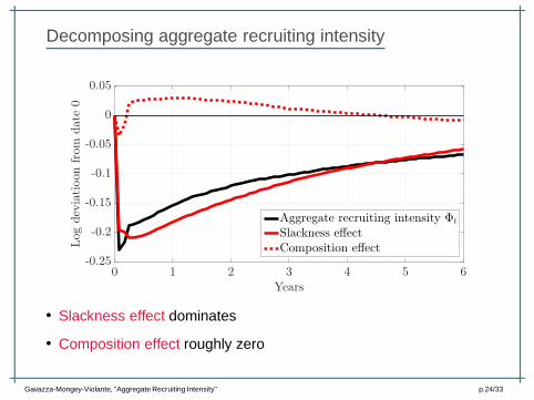
Decomposing aggregate recruiting intensityyl
0 1 2 3 4 5 6Years
-0.25
-0.2
-0.15
-0.1
-0.05
0
0.05Logdeviatioonfrom
date
0
Aggregate recruiting intensity Φt
Slackness effectComposition effect
• Slackness effect dominates
• Composition effect roughly zero
Gavazza-Mongey-Violante, "Aggregate Recruiting Intensity" p.24/33hello
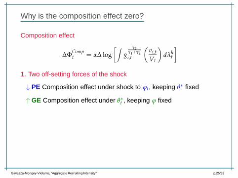
Why is the composition effect zero?yl
Composition effect
∆ΦCompt = α∆ log
[∫
g
γ2γ1+γ2i,t
(vi,t
Vt
)
dλht
]
1. Two off-setting forces of the shock
↓ PE Composition effect under shock to ϕt, keeping θ∗ fixed
↑ GE Composition effect under θ∗t , keeping ϕ fixed
Gavazza-Mongey-Violante, "Aggregate Recruiting Intensity" p.25/33hello
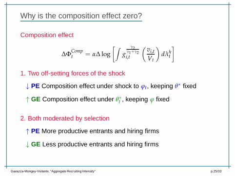
Why is the composition effect zero?yl
Composition effect
∆ΦCompt = α∆ log
[∫
g
γ2γ1+γ2i,t
(vi,t
Vt
)
dλht
]
1. Two off-setting forces of the shock
↓ PE Composition effect under shock to ϕt, keeping θ∗ fixed
↑ GE Composition effect under θ∗t , keeping ϕ fixed
2. Both moderated by selection
↑ PE More productive entrants and hiring firms
↓ GE Less productive entrants and hiring firms
Gavazza-Mongey-Violante, "Aggregate Recruiting Intensity" p.25/33hello
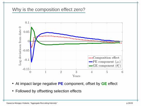
Why is the composition effect zero?yl
0 1 2 3 4 5 6Years
-0.15
-0.1
-0.05
0
0.05
0.1Logdeviatioonfrom
date
0
Composition effectPE component (ϕt)GE component (θ∗t )
• At impact large negative PE component, offset by GE effect
• Followed by offsetting selection effects
Gavazza-Mongey-Violante, "Aggregate Recruiting Intensity" p.26/33hello
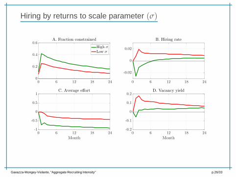
Hiring by returns to scale parameter (σ)yl
0 6 12 18 240
0.2
0.4
0.6A. Fraction constrained
High σ
Low σ
0 6 12 18 24
-0.02
0
0.02
B. Hiring rate
0 6 12 18 24
Month
-1
-0.5
0
0.5
1C. Average effort
0 6 12 18 24
Month
-0.2
-0.1
0
0.1
0.2D. Vacancy yield
Gavazza-Mongey-Violante, "Aggregate Recruiting Intensity" p.26/33hello
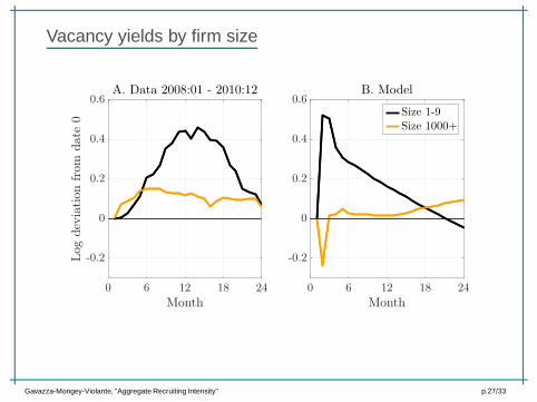
Vacancy yields by firm sizeyl
0 6 12 18 24
Month
-0.2
0
0.2
0.4
0.6
Log
deviation
from
date0
A. Data 2008:01 - 2010:12
0 6 12 18 24
Month
-0.2
0
0.2
0.4
0.6B. Model
Size 1-9Size 1000+
Gavazza-Mongey-Violante, "Aggregate Recruiting Intensity" p.27/33hello
Taking stock and going forwardyl
Answers
1. Recruiting intensity explains approx. 1/3 of decline in match eff.
2a. Dominant effect: Slack markets reduce need for costly recruiting
2b. Strong selection effects limit role of compositional changes
2 . Slackness and composition explain vacancy yields by size
Gavazza-Mongey-Violante, "Aggregate Recruiting Intensity" p.28/33hello
Taking stock and going forwardyl
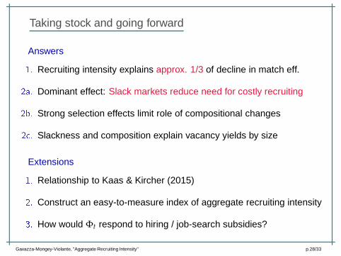
Answers
1. Recruiting intensity explains approx. 1/3 of decline in match eff.
2a. Dominant effect: Slack markets reduce need for costly recruiting
2b. Strong selection effects limit role of compositional changes
2 . Slackness and composition explain vacancy yields by size
Extensions
1. Relationship to Kaas & Kircher (2015)
2. Construct an easy-to-measure index of aggregate recruiting intensity
3. How would Φt respond to hiring / job-search subsidies?
Gavazza-Mongey-Violante, "Aggregate Recruiting Intensity" p.28/33hello
1. Relation to Kaas Kircher (2015)yl
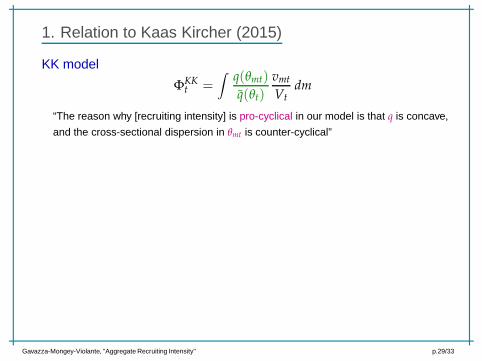
KK model
ΦKKt =
∫q(θmt)
q(θt)
vmt
Vtdm
“The reason why [recruiting intensity] is pro-cyclical in our model is that q is concave,
and the cross-sectional dispersion in θmt is counter-cyclical”
Gavazza-Mongey-Violante, "Aggregate Recruiting Intensity" p.29/33hello
1. Relation to Kaas Kircher (2015)yl
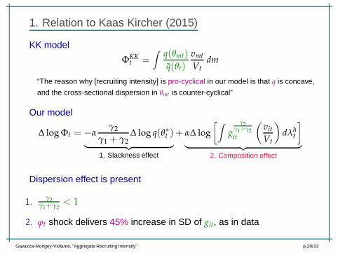
KK model
ΦKKt =
∫q(θmt)
q(θt)
vmt
Vtdm
“The reason why [recruiting intensity] is pro-cyclical in our model is that q is concave,
and the cross-sectional dispersion in θmt is counter-cyclical”
Our model
∆ log Φt = −αγ2
γ1 + γ2∆ log q(θ∗t )
︸ ︷︷ ︸
1. Slackness effect
+ α∆ log
[∫
g
γ2γ1+γ2it
(vit
Vt
)
dλht
]
︸ ︷︷ ︸
2. Composition effect
Dispersion effect is present
1.
γ2γ1+γ2
< 1
2. ϕt shock delivers 45% increase in SD of git, as in data
Gavazza-Mongey-Violante, "Aggregate Recruiting Intensity" p.29/33hello
1. Relation to Kaas Kircher (2015)yl
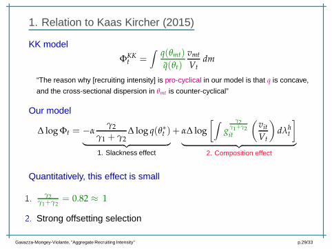
KK model
ΦKKt =
∫q(θmt)
q(θt)
vmt
Vtdm
“The reason why [recruiting intensity] is pro-cyclical in our model is that q is concave,
and the cross-sectional dispersion in θmt is counter-cyclical”
Our model
∆ log Φt = −αγ2
γ1 + γ2∆ log q(θ∗t )
︸ ︷︷ ︸
1. Slackness effect
+ α∆ log
[∫
g
γ2γ1+γ2it
(vit
Vt
)
dλht
]
︸ ︷︷ ︸
2. Composition effect
Quantitatively, this effect is small
1.
γ2γ1+γ2
= 0.82 ≈ 1
2. Strong offsetting selection
Gavazza-Mongey-Violante, "Aggregate Recruiting Intensity" p.29/33hello
2. Approximate index of aggregate recruiting intensityyl
Gavazza-Mongey-Violante, "Aggregate Recruiting Intensity" p.30/33hello
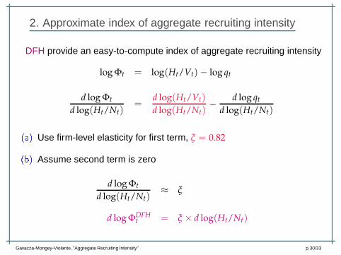
2. Approximate index of aggregate recruiting intensityyl
DFH provide an easy-to-compute index of aggregate recruiting intensity
log Φt = log(Ht/Vt)− log qt
d log Φt
d log(Ht/Nt)=
d log(Ht/Vt)
d log(Ht/Nt)−
d log qt
d log(Ht/Nt)
(a) Use firm-level elasticity for first term, ξ = 0.82
(b) Assume second term is zero
d log Φt
d log(Ht/Nt)≈ ξ
d log ΦDFHt = ξ × d log(Ht/Nt)
Gavazza-Mongey-Violante, "Aggregate Recruiting Intensity" p.30/33hello
2. Approximate index of aggregate recruiting intensityyl
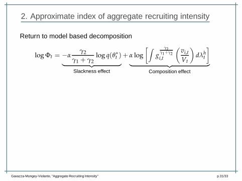
Return to model based decomposition
log Φt = −αγ2
γ1 + γ2log q(θ∗t )
︸ ︷︷ ︸
Slackness effect
+ α log
[∫
g
γ2γ1+γ2i,t
(vi,t
Vt
)
dλht
]
︸ ︷︷ ︸
Composition effect
Gavazza-Mongey-Violante, "Aggregate Recruiting Intensity" p.31/33hello
2. Approximate index of aggregate recruiting intensityyl
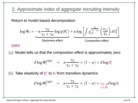
Return to model based decomposition
log Φt = −αγ2
γ1 + γ2log q(θ∗t )
︸ ︷︷ ︸
Slackness effect
+ α log
[∫
g
γ2γ1+γ2i,t
(vi,t
Vt
)
dλht
]
︸ ︷︷ ︸
Composition effect
GMV
(a) Model tells us that the composition effect is approximately zero
d log ΦGMVt = α
γ2
γ1 + γ2× (1 − α)× d log θ∗t
(b) Take elasticity of θ∗t to θt from transition dynamics
d log ΦGMVt = α
γ2
γ1 + γ2× (1 − α)× εθ∗,θ
≈1.45
d log θt
Gavazza-Mongey-Violante, "Aggregate Recruiting Intensity" p.31/33hello
2. Approximate index of aggregate recruiting intensityyl
2001 2002 2003 2004 2005 2006 2007 2008 2009 2010 2011 2012 2013 2014-0.5
-0.4
-0.3
-0.2
-0.1
0
0.1
0.2
Log
Aggregate
RecruitingIntensity
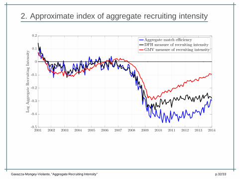
Aggregate match efficiencyDFH measure of recruiting intensityGMV measure of recruiting intensity
Gavazza-Mongey-Violante, "Aggregate Recruiting Intensity" p.32/33hello
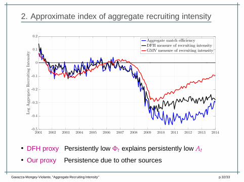
2. Approximate index of aggregate recruiting intensityyl
2001 2002 2003 2004 2005 2006 2007 2008 2009 2010 2011 2012 2013 2014-0.5
-0.4
-0.3
-0.2
-0.1
0
0.1
0.2
Log
Aggregate
RecruitingIntensity
Aggregate match efficiencyDFH measure of recruiting intensityGMV measure of recruiting intensity
• DFH proxy Persistently low Φt explains persistently low At
• Our proxy Persistence due to other sources
Gavazza-Mongey-Violante, "Aggregate Recruiting Intensity" p.32/33hello
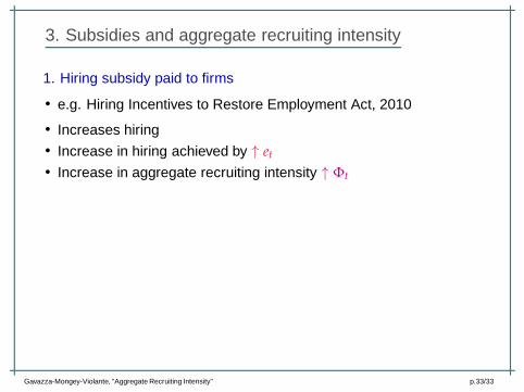
3. Subsidies and aggregate recruiting intensityyl
1. Hiring subsidy paid to firms
• e.g. Hiring Incentives to Restore Employment Act, 2010
• Increases hiring• Increase in hiring achieved by ↑ et
• Increase in aggregate recruiting intensity ↑ Φt
Gavazza-Mongey-Violante, "Aggregate Recruiting Intensity" p.33/33hello
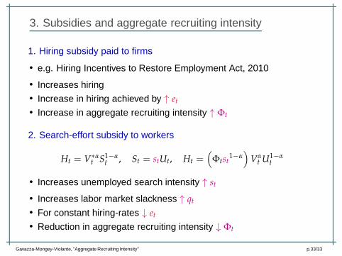
3. Subsidies and aggregate recruiting intensityyl
1. Hiring subsidy paid to firms
• e.g. Hiring Incentives to Restore Employment Act, 2010
• Increases hiring• Increase in hiring achieved by ↑ et
• Increase in aggregate recruiting intensity ↑ Φt
2. Search-effort subsidy to workers
Ht = V∗αt S1−α
t , St = stUt, Ht =(
Φtst1−α
)
Vαt U1−α
t
• Increases unemployed search intensity ↑ st
• Increases labor market slackness ↑ qt
• For constant hiring-rates ↓ et
• Reduction in aggregate recruiting intensity ↓ Φt
Gavazza-Mongey-Violante, "Aggregate Recruiting Intensity" p.33/33hello
yl
THANK YOU!
Gavazza-Mongey-Violante, "Aggregate Recruiting Intensity" p.33/33hello
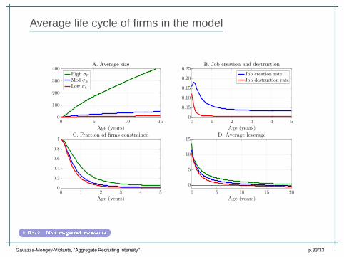
Average life cycle of firms in the modelyl
0 1 2 3 4 5
Age (years)
0
0.05
0.10
0.15
0.20
0.25B. Job creation and destruction
Job creation rateJob destruction rate
0 5 10 15
Age (years)
0
100
200
300
400A. Average size
High σH
Med σM
Low σL
0 1 2 3 4 5
Age (years)
0
0.2
0.4
0.6
0.8
1C. Fraction of firms constrained
0 5 10 15 20
Age (years)
0
5
10
15D. Average leverage
Ba k - Non-targetted moments
Gavazza-Mongey-Violante, "Aggregate Recruiting Intensity" p.33/33hello
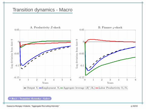
Transition dynamics - Macroyl
0 1 2 3 4 5 6Years
-0.15
-0.1
-0.05
0
0.05
Logdeviationfrom
date
0
A. Productivity Z-shock
0 1 2 3 4 5 6Years
-0.15
-0.1
-0.05
0
0.05
Logdeviationfrom
date
0
B. Finance ϕ-shock
Output Yt Employment Nt Aggregate leverage (B+t /Kt) Labor Productivity Yt/Nt
Ba k - Transition dynami s - Labor
Gavazza-Mongey-Violante, "Aggregate Recruiting Intensity" p.33/33hello