RUHRECONOMIC PAPERS

Gold as an Infl ation Hedge in a

Time-Varying Coeffi cient Framework

#362

Joscha BeckmannRobert Czudaj

Imprint

Ruhr Economic Papers

Published by

Ruhr-Universität Bochum (RUB), Department of EconomicsUniversitätsstr. 150, 44801 Bochum, Germany

Technische Universität Dortmund, Department of Economic and Social SciencesVogelpothsweg 87, 44227 Dortmund, Germany

Universität Duisburg-Essen, Department of EconomicsUniversitätsstr. 12, 45117 Essen, Germany

Rheinisch-Westfälisches Institut für Wirtschaftsforschung (RWI)Hohenzollernstr. 1-3, 45128 Essen, Germany

Editors

Prof. Dr. Thomas K. BauerRUB, Department of Economics, Empirical EconomicsPhone: +49 (0) 234/3 22 83 41, e-mail: thomas.bauer@rub.de

Prof. Dr. Wolfgang LeiningerTechnische Universität Dortmund, Department of Economic and Social SciencesEconomics – MicroeconomicsPhone: +49 (0) 231/7 55-3297, email: W.Leininger@wiso.uni-dortmund.de

Prof. Dr. Volker ClausenUniversity of Duisburg-Essen, Department of EconomicsInternational EconomicsPhone: +49 (0) 201/1 83-3655, e-mail: vclausen@vwl.uni-due.de

Prof. Dr. Christoph M. SchmidtRWI, Phone: +49 (0) 201/81 49-227, e-mail: christoph.schmidt@rwi-essen.de

Editorial Offi ce

Joachim SchmidtRWI, Phone: +49 (0) 201/81 49-292, e-mail: joachim.schmidt@rwi-essen.de

Ruhr Economic Papers #362

Responsible Editor: Volker Clausen

All rights reserved. Bochum, Dortmund, Duisburg, Essen, Germany, 2012

ISSN 1864-4872 (online) – ISBN 978-3-86788-416-7The working papers published in the Series constitute work in progress circulated to stimulate discussion and critical comments. Views expressed represent exclusively the authors’ own opinions and do not necessarily refl ect those of the editors.

Ruhr Economic Papers #362

Joscha Beckmann and Robert Czudaj

Gold as an Infl ation Hedge in a

Time-Varying Coeffi cient Framework

Bibliografi sche Informationen

der Deutschen Nationalbibliothek

Die Deutsche Bibliothek verzeichnet diese Publikation in der deutschen National-bibliografi e; detaillierte bibliografi sche Daten sind im Internet über: http://dnb.d-nb.de abrufb ar.

http://dx.doi.org/10.4419/86788416ISSN 1864-4872 (online)ISBN 978-3-86788-416-7

Joscha Beckmann and Robert Czudaj1

Gold as an Infl ation Hedge in a

Time-Varying Coeffi cient Framework

Abstract

This study analyzes the question whether gold provides the ability of hedging against infl ation from a new perspective. Using data for four major economies, namely the USA, the UK, the Euro Area, and Japan, we allow for nonlinearity and discriminate between long-run and time-varying short-run dynamics. Thus, we conduct a Markov-switching vector error correction model (MS-VECM) approach for a sample period ranging from January 1970 to December 2011. Our main fi ndings are threefold: First, we show that gold is partially able to hedge future infl ation in the long-run and this ability is stronger for the USA and the UK compared to Japan and the Euro Area. In addition, the adjustment of the general price level is characterized by regime-dependence, implying that the usefulness of gold as an infl ation hedge for investors crucially depends on the time horizon. Finally, one regime approximately accounts for times of turbulences while the other roughly corresponds to ’normal times’.

JEL Classifi cation: C32, E31, E44

Keywords: Cointegration; gold price; infl ation hedge; Markov-switching error correction; price level

August 2012

1 Joscha Beckmann, University of Duisburg-Essen, Department of Economics, Chair for Macroeconomics; Robert Czudaj, University of Duisburg-Essen, Department of Economics, Chair for Statistics and Econometrics; FOM Hochschule für Oekonomie & Management, University of Applied Sciences. – Thanks for valuable comments are due to Fátima Sol and the participants of the 14th INFER Annual Conference, University of Coimbra/Portugal. – All correspondence to: Robert Czudaj, University of Duisburg-Essen, Universitätsstr. 12, D-45117 Essen, Germany. E-mail: robert.czudaj@uni-due.de.

4

1 Introduction

Although gold is no longer a central cornerstone of the international monetary system since

the breakdown of Bretton Woods, it still attracts considerable interest from both investors

and researchers. Owing to the increasing complexity of financial markets, diversifying a port-

folio through hedging has become increasingly important. In a nutshell, gold may act as a

hedge or ’safe haven’ asset for portfolio investors.1 The majority of academic research has fo-

cused on the first property since a widespread consensus states that the price of gold reflects

inflation expectations. One reason is that commodity prices are generally considered to be

able to incorporate new information faster than consumer prices (Mahdavi and Zhou, 1997).

Gold prices seem to be appropriate regarding the reflection of inflation expectations since,

in contrast to many other commodities, gold is durable, relatively transportable, universally

acceptable and easily authenticated (Worthington and Pahlavani, 2007). From a theoretical

point of view, an increase in expected inflation will force investors to buy gold, either to hed-

ge against the expected decline in the value of money or to speculate due to the associated

rise of the gold price. This generates a purchasing pressure which yields to an immediately

rising price of gold in time of the upward revision in inflation expectations. Thus, changes in

expected inflation will cause changes in the price of gold and investors with knowledge regar-

ding future inflation have the ability to gain excess revenues by purchasing and selling gold

in spot and futures markets in anticipation of prospective market adjustments. Therefore,

the gold price acts as a leading indicator of the level of inflation and hence, gold could be

used to hedge against future inflation. This causality pattern has recently been questioned

by Blose (2010) who argues that the costs of carrying gold are also affected through changes

in interest rates by expected inflation. If those costs offset revenues from speculation, the

price of gold is not affected by changing inflation expectations.2

To understand the main characteristics of gold prices, a brief description of supply and de-

mand factors is necessary. According to Baur and McDermott (2010) and the World Gold

Council the supply of gold, such as the supply of other commodities, is relatively inelastic,

owing to the difficult extraction process and the tedious establishment of new mines.3 Cen-

tral banks also still keep maintaining passive stocks of gold, independently of the patterns of

the real price of gold (Aizenman and Inoue, 2012). Hence, the gold supply remains relatively

stable while the gold demand is rapidly changing in response to global economic occurrences.

1Gold has also retained its unique status in central bank portfolios (Aizenman and Inoue, 2012).2Blose (2010) labels this view as the carrying costs hypothesis while he corresponds to the expected inflationhypothesis as the opposite view.

3Although the gold supply is inelastic to prices it has not been constant over the whole sample period underobservation. It actually peaked in 2001.

5

Following Baur and McDermott (2010) the total demand for gold can be separated in three

categories: demand for jewelry, demand for industrial and dental, and investment demand.

While demand for jewelry as well as for industrial and dental is largely determined by con-

sumer spending power and thus, attached to the business cycle, the investment demand for

gold could act counter-cyclical due to an increased demand for gold in times of global crises

and recessions. Ghosh et al. (2004) merely divide the total gold demand in two categories,

namely the ’use demand’ which combines the first two categories mentioned above and the

’asset demand’, where gold is also used by governments, fund managers and individuals as

an investment to hedge inflation and other forms of uncertainty.

Although gold may act as an inflation hedge in the long-run, the price for gold also displays

significant short-run price volatility (Aggarwal, 1992). Hence, cointegration techniques seem

to be the appropriate tools to examine the relationship between consumer prices and the

price for gold. Those frameworks are based on the idea of a stable long-run equilibrium re-

lation between the prices for goods and services and for gold while the variables are allowed

to depart from their equilibrium path in the short-run due to random shocks in the spirit of

Engle and Granger (1987). The adjustment coefficients correspond to the speed of correction

of short-run deviations from the long-run equilibrium. In this vein, many previous studies

have focused on the inflation hedging ability of gold by partly applying conventional cointe-

gration frameworks (Kolluri, 1981; Moore, 1990; Laurent, 1994; Chappell and Dowd, 1997;

Mahdavi and Zhou, 1997; Harmston, 1998; Ghosh et al., 2004; Levin and Wright, 2006).

However, the relationship between consumer prices and gold prices has undergone several

structural changes since the early seventies: the breakdown of Bretton Woods in 1973, two

major oil price shocks in 1973 and 1979/80, the collapse of the USSR in 1991 and the sub-

sequent democratization of Russia as one of the top producer of gold worldwide, the burst

of the ’dot-com bubble’ in 2001 and the recent financial and economic crises that started

in 2007.4 Hence, due to the frequent changes in the equilibrium relationships the parameter

constancy assumption of the traditional VECM methodology seems to be too restrictive.

Worthington and Pahlavani (2007) argue that ignoring such substantial changes could yield

to the inability of proving the existence of a stable long-run relationship between consumer

prices and the price for gold.

However, to the best of our knowledge the only study which considers the possibility of non-

linearity in the inflation hedging relation is provided by Wang et al. (2011).5 They argue that

4In addition, gold price controls were not completely phased out in the U.S. until the mid 1970’s.5Kyrtsou and Labys (2006) also show that the nature of the dependence and the causal relation between U.S.inflation and commodity prices can be characterized by nonlinearity using nonlinear Granger causality

6

the existence of transaction costs and the above mentioned business cycle dependence of the

gold demand possibly results in a nonlinear relationship between consumer prices and gold

prices. For this reason, they account for nonlinearity based on the threshold cointegration

framework developed by Enders and Siklos (2001). From a methodological point of view,

such a framework adequately describes the dynamics if the data is primarily generated by

market forces since the regime variable is assumed to be endogenous (Balke and Fomby,

1997; Enders and Siklos, 2001; Lo and Zivot, 2001; Hansen and Seo, 2002). However, if gold

acts as an inflation hedge, exogenous factors such as major economic shocks or changes in

economic policy may have an influence on the path of the gold prices. In that case, a Markov-

switching vector error correction model (MS-VECM), where the unobservable state follows

an exogenous stochastic process, is more suitable compared to a conventional threshold mo-

del (Ihle and von Cramon-Taubadel, 2008). This is also reasonable from an economic point

view since choosing a specific transition variable may also indicate a certain causality since

the adjustment pattern depends on the chosen threshold.

Hence, the rational for this study is to contribute to the literature by adopting a MS-VECM

approach when analyzing whether gold provides the ability of hedging inflation in four major

countries, namely the USA, the UK, the Euro Area, and Japan. We allow for nonlinearity

and discriminate between long-run and time-varying short-run dynamics. Strictly speaking,

the benefit of our framework is that it allows identifying the potentially latent regimes in the

data and helps to specify the nonlinear dynamics between the variables adequately. More

precisely, we are able to provide a measure of usefulness for an inflation hedge over different

time periods by analyzing the time-varying price adjustment for different subperiods.

The reminder of this paper is organized as follows. The following section provides a brief

summary of previous empirical findings. Section 3 describes our data as well as our empirical

framework. The results are presented and analyzed in section 4. Section 5 concludes.

2 Literature review

The dynamics of the price for gold has been focused by academic literature in many respects

over the last decades. The first literature strand consists of studies which address impacts

of macroeconomic variables such as exchange rates, interest rates, or output on the price

for gold. Studies of this kind have been provided by Sherman (1982, 1983), Ariovich (1983),

Fortune (1987), Dooley et al. (1995), Sjaastad and Scacciallani (1996), Lucey et al. (2006),

tests.

7

and Wang and Lee (2011). Focusing on a different topic, Koutsoyiannis (1983), Diba and

Grossman (1984), Baker and van Tassel (1985), and Pindyck (1993) deal with the ability to

forecast the gold price. Generally speaking, evidence for different relationships and causa-

lities including the price of gold has been provided. However, a detailed description of the

corresponding results is beyond the scope of this paper.

Focusing on the recent increase in gold prices, Bialkowski et al. (2011) test whether a specu-

lative bubble in the price of gold exists by applying a Markov regime-switching augmented

Dickey-Fuller test and conclude that the high current gold price seems to be fundamentally

justified. Tests of the market efficiency hypothesis for gold markets have been undertaken by

Tschoegl (1980), Solt and Swanson (1981), Ho (1985), Basu and Clouse (1993), and Smith

(2002). Another frequently analyzed research topic is the capability of gold as a hedge or

a ’safe haven’ with regard to financial assets such as bonds or stocks.6 Such a question has

been tackled by Sherman (1986), Jaffe (1989), Chua et al. (1990), Ciner (2001), Michaud et

al. (2006), Hillier et al. (2006), McCown and Zimmerman (2006), Baur and Lucey (2010),

Baur and McDermott (2010), and Ciner et al. (2010). Capie et al. (2005) examine whether

gold could be a hedge against fluctuations of the U.S. dollar. The overall results are mixed

with recent results suggesting that gold is only able to provide a ’safe haven’ function in the

very short-run (Baur and Lucey, 2010).7

Finally, studies which are most closely related to our topic have analyzed the linkages bet-

ween inflation and the price for gold. Kolluri (1981), Moore (1990), Laurent (1994), Chappell

and Dowd (1997), Mahdavi and Zhou (1997), Harmston (1998), Ghosh et al. (2004), Levin

and Wright (2006), Worthington and Pahlavani (2007) and Wang et al. (2011) examine the

inflation hedge effectiveness of gold by focusing on the short-run and the long-run relation-

ship between the general price level and the price for gold. It is worth mentioning that studies

which focus on ’safe haven’ aspects mostly adopt daily instead of monthly data. The results

which will briefly be described in the following are not clear-cut and vary depending on the

sample period and the country under observation. In an early study, Mahdavi and Zhou

(1997) tackle the question whether gold and other commodity prices are leading indicators

of inflation based on the estimation of a conventional VECM for the USA using the Johan-

sen (1988, 1991) framework for a quarterly sample period that ranges from 1970 to 1994

6Baur and Lucey (2010) define a hedge and a ’safe haven’ as an asset that is uncorrelated or negativelycorrelated with another asset or portfolio on average and only in times of market stress or turmoil,respectively.

7Aizenman and Inoue (2012) also point out that central bank’s gold position signals economic might, andthat gold retains the stature of a ’safe haven’ asset at times of global turbulence.

8

and conclude that consumer prices and the price of gold are not cointegrated. Thus, their

outcomes are in line with the findings of Garner (1995) and Cecchetti et al. (2000) who were

unable to provide empirical evidence for the usefulness of the gold price as leading indicator

for inflation as well.8 On the contrary, Laurent (1994), Harmston (1998) and Ghosh et al.

(2004) detect an effective long-run inflation hedge of gold in the USA, the UK, France, Ger-

many, and Japan. Ghosh et al. (2004) use monthly U.S. data that ranges from 1976 to 1999

and apply cointegration regression techniques. Adrangi et al. (2003) find that gold prices are

positively correlated with expected inflation and conclude that a gold investment may be

a reliable inflation hedge in both the short-run and the long-run. Levin and Wright (2006)

also estimate a conventional VECM to analyze the short-run and long-run determinants of

the gold price for the USA over a sample period from 1976 to 2005. They identify a stable

long-run relationship between the gold price and the price level. Their findings also provide

evidence that the change in the gold price is positively related to the change in inflation,

inflation volatility, and credit risk while a negative relationship with regard to the U.S. dollar

trade weighted exchange rate and the gold lease rate prevails. Using monthly data spanning

the period from September 1994 to December 2005 for 14 countries (Australia, Canada,

the European Union, New Zealand, Sweden, the United Kingdom, Japan, Mexico, Norway,

the USA, Brazil, China, India, and Israel) Tkacz (2007) finds that the gold price contains

significant information for future inflation in several countries, especially in those that have

adopted formal inflation targets.

Worthington and Pahlavani (2007) also test the presence of a stable long-run relationship

between the price of gold and inflation in the USA using monthly data from 1945 to 2006 and

from 1973 to 2006. However, they additionally allow for instabilities when analyzing the long-

run relation. In their framework, the timing of structural breaks is endogenously determined

by applying the unit root testing procedure developed by Zivot and Andrews (1992) and

thereafter a modified cointegration approach suggested by Saikkonen and Lutkepohl (2000a,

2000b, 2000c) is adopted. The results provide evidence in favor of a cointegrating relation-

ship between the price of gold and inflation in both sample periods and thus, Worthington

and Pahlavani (2007) conclude that a gold investment can serve as an effective inflationary

hedge. Finally, Wang et al. (2011) have analyzed the short-run and long-run inflation hed-

ging effectiveness of gold in the USA and Japan for a sample period ranging from January

1971 to January 2010 while using monthly data. They conduct the linear cointegration test

proposed by Engle and Granger (1987) as well as the nonlinear threshold cointegration test

8Furthermore, Tully and Lucey (2007) have applied a power GARCH approach and also do not find asignificant relationship between gold prices and inflation.

9

suggested by Enders and Siklos (2001) and show that in low momentum regimes gold is

unable to hedge against inflation in both the USA and Japan, however, in high momentum

regimes, a gold investment is able to hedge against inflation in the USA, and partially hedge

against inflation in Japan.

Summing up the empirical evidence, the ambiguous results of previous studies as well as

the provided evidence for instabilities in the relationship between gold prices and inflation

verify the application of a time-varying Markov-switching approach. In our analysis, the

long-run coefficients indicate the intensity of a relationship between the price for gold and

the general price level. However, gold is only useful as a hedge if prices adjust to deviations

from such a long-run relationship. In this case, the long-run estimates also provide a measure

of effectiveness of an inflation hedge. Hence, in our framework the time-varying adjustment

coefficients are able to discriminate between periods with and without hedging functions. If

prices do not adjust, buying gold may not be able to shield a portfolio with respect to future

price movements during a specific period.

3 Data and econometric methodology

3.1 Data

We use a monthly dataset including the price for gold denominated in U.S. Dollar, British

Pound Sterling, Euro and Japanese Yen as well as the consumer price index (CPI) and the

producer price index (PPI) of the USA, the UK, the Euro Area, and Japan. Using two

different measures of inflation includes a robustness test for our results and also allows for

different hedging abilities of gold for consumers and producers.9

The gold price data has been provided by the World Gold Council and covers a sample pe-

riod from December 1969 to December 2011. Hence, we also include the period immediately

before the breakdown of Bretton Woods. The CPI’s (2005=100) and the PPI’s (2000=100)

for the USA, the UK, and Japan have been taken from the statistics provided by the OECD

and the IMF, respectively. Both the CPI (2005=100) as well as the PPI (2005=100) for

the Euro Area are taken from the ECB Statistical Data Warehouse and cover only a period

ranging from February 1980 to November 2011 and from January 1981 to November 2011,

respectively. The country selection is motivated by the fact that the currencies of the chosen

four major economies are regarded as key currencies by the World Gold Council. As it is

9While most studies regarding the relationship between inflation and gold prices such as, for instance, Wanget al. (2011) use the CPI to construct a measure of inflation, Lawrence (2003) adopts the PPI.

10

common practice, each series is taken as natural logarithm.

In order to analyze the underlying long-run dynamics using bi-variate cointegration tech-

niques, it is important to assure that the times series under observation are integrated of

the same order. In the present context, an important question is whether some variables,

in particular prices, are integrated of order two, e.g. I(2). The results of the augmented

Dickey-Fuller (ADF) test and the more powerful Ng-Perron MZα test suggest that all series

may be approximated as integrated of order one, e.g. I(1) (Dickey and Fuller, 1979; Ng and

Perron, 2001).10

3.2 Econometric methodology

In the following we use a Markov-switching vector error correction model (MS-VECM) to

examine the relationship between the price for gold (gt) and the CPI as well as PPI (pt) for

the set of the four countries mentioned above. The concept of the MS-VECM is based on

traditional state-dependent time series models developed by Hamilton (1989) and continued

by Krolzig (1997). As will be described below, the parameters of a MS-VECM are designed

to take a constant value in each regime and to shift discretely from one regime to the

other with different switching probabilities. The switches between different states are not

accounted as deterministic occurrences, but are assumed to follow an exogenous stochastic

process. Consider a M -regime pth order MS-VECM, which in general allows for regime

shifts in the vector of intercept terms, the autoregressive part, the long-run matrix, and the

variance-covariance matrix of the errors:11

ΔYt = v(st) + Γ(L)(st)ΔYt−l +Π(st)Yt−1 + εt, t = 1, . . . , T, (1)

where Δ denotes the difference operator, Yt represents aK-dimensional vector of the observed

time series, Yt = [pt, gt]′; v(st) denominates a K-dimensional vector of regime-dependent in-

tercept terms, v(st) = [v1(st), . . . , vK(st)]′, while εt = [ε1t, . . . , εKt]

′ describes aK-dimensional

vector of error terms with regime-dependent variance-covariance matrix Σ(st), εt ∼ NIID(0,

Σ(st)). The K ×K matrix lag polynomial Γ(L)(st) of order p denotes the state-dependent

short-run dynamics of the model. The stochastic regime-generating process is assumed to

be an ergodic, homogenous and irreducible first-order Markov chain with a finite number of

10We apply an auxiliary regression either with a constant or with a linear trend plus constant since agraphical inspection shows that most of the series exhibit a time dependent mean. The results of the unitroot tests are available upon request.

11This model is often referred to as Markov-Switching-Intercept-Autoregressive-Heteroskedastic-VECM orMSIAH-VECM. See Sarno and Valente (2006) among others.

11

regimes, st ∈ {1, . . . ,M}, and constant transition probabilities12

pij = Pr(st+1 = j|st = i), pij > 0,M∑

j=1

pij = 1 ∀ i, j ∈ {1, . . . ,M} . (2)

The first expression of equation (2) gives the probability for switching from regime i to re-

gime j at time t + 1 which is independent of the history of the process. pij is the element

in the ith row and the jth column of the M ×M matrix of the transition probabilities P ,

which is usually not symmetric.

The non-stationary behavior of the series is accounted for by a reduced rank (r < K) re-

striction of the state-dependent K×K long-run level matrix Π(st), which can be fragmented

into two K × r matrices α(st) and β such that Π(st) = α(st)β′. β′ gives the coefficients of

the variables for the r long-run relations which are assumed to be constant over the whole

sample period, while α(st) contains the regime-dependent adjustment coefficients describing

the reaction of each variable to disequilibria from the r long-run relations given by the

r-dimensional vector β′Yt−1. Thus, in our model the most interesting distinction between

regimes is the speed in which deviations from the long-run equilibrium are corrected given

by α(st).

First, in order to identify the rank of Π(st), e.g. the number of cointegrating relations r, and to

estimate the coefficients of the r cointegrating vectors in β′ we rely on a framework developed

by Johansen (1988, 1991). Then, conditional on these cointegrating vectors, the regime-

dependent adjustment parameters α(st), intercept terms v(st), autoregressive coefficients

Γ(L)(st), and variance-covariance matrix Σ(st) as well as the transition probabilities are

estimated using a Markov Chain Monte Carlo (MCMC) method, namely the multi-move

iterative Gibbs sampling procedure proposed by Krolzig (1997).13 This two-step framework

is adopted from the work of Saikkonen (1992) as well as Saikkonen and Luukkonen (1997)

12The ergodicity assumption implies a stationary unconditional probability distribution of the regimes,the homogeneity assumption defines the transition probabilities to be constant, and finally, the irre-ducibility assumption assures that any regime can be reached from any other regime (Ihle and vonCramon-Taubadel, 2008).

13The Gibbs sampling technique goes back to Geman and Geman (1984) and has been extended to univariateMarkov-switching models by Albert and Chib (1993), McCulloch and Tsay (1994), and Filardo (1994).An alternative procedure is the expectation-maximization (EM) algorithm for maximum likelihood esti-mation which has been applied, for instance, by Sarno and Valente (2006). See Dempster et al. (1977),Hamilton (1993), Krolzig (1997), and Kim and Nelson (1999) for details. Although, the EM algorithmrequires fewer computations, it does not directly provide the posterior distribution of the parameters andestimates of the variance-covariance matrix of the errors (Krolzig, 1997). To check for robustness we haveused the EM algorithm as well. Our results turned out to be reliable.

12

who showed that the Johansen procedure provides consistent estimates for the cointegrating

vectors even in the presence of regime-switching.14

4 Empirical results

With respect to the deterministic components of a VECM, Johansen (1988) distinguishes five

different specifications. In this vein, an important question is whether deterministic trends

are obtained in the data and whether they cancel out in the long-run relationships. Since

both the price of gold as well as consumer and producer prices may include such trends,

we consider two trend specifications for each model, both allowing for a linear deterministic

trend in the data. The first configuration also includes a trend in the cointegration space,

implying that the underlying deterministic trends of the general price level and the price

for gold do not cancel out in the long-run relationship. The second setting corresponds to

the case where the trends do cancel out. In this case, not a trend but an unrestricted con-

stant is included since each of our series shows a time dependent mean. In the following, all

long-run estimations for both CPI and PPI are carried out for both configurations. In terms

of robustness, this proceeding assures that the detection of a long-run relationship does not

depend on the specification of the deterministic components. However, since the significance

of a trend in the long-run relationship can be tested, we base our analysis of the time-varying

short-run dynamics on the more adequate specification.

The choice of the lag length p of each model is based on the Schwarz criterion and tests for

autocorrelation and ARCH effects. According to Rahbek et al. (2002), the rank test results

we gain in the following are still robust under the remaining ARCH effects in some cases.

While excess kurtosis does not introduce a significant bias to the estimated cointegrating

vectors the findings are sensitive to excess skewness (Juselius and MacDonald, 2004; Juselius,

2006). After introducing dummy variables to account for outliers following the methodology

described in Juselius (2006), the rejection of the normality assumption is solely due to excess

kurtosis, so that our results are still reliable. The corresponding statistics are available upon

request.

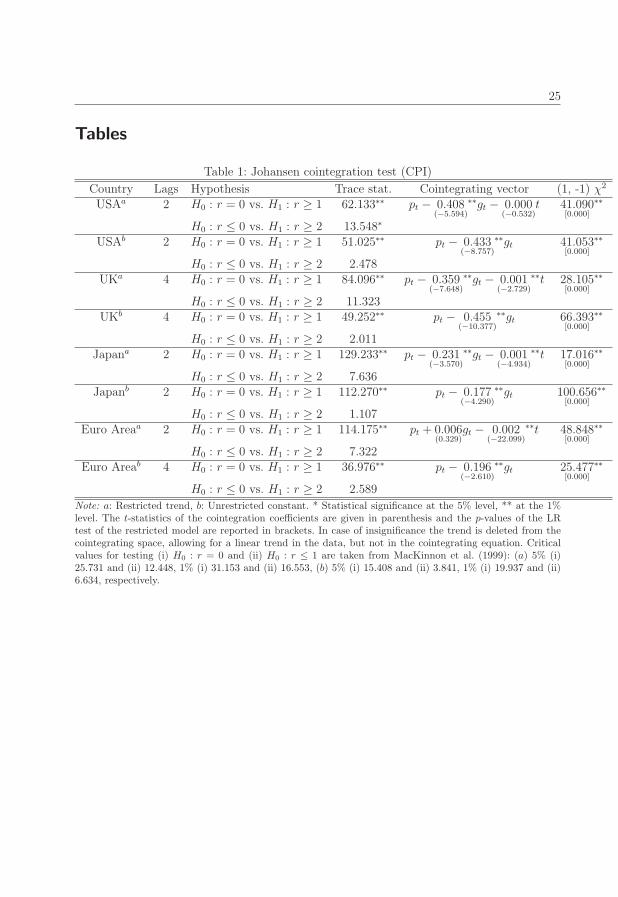
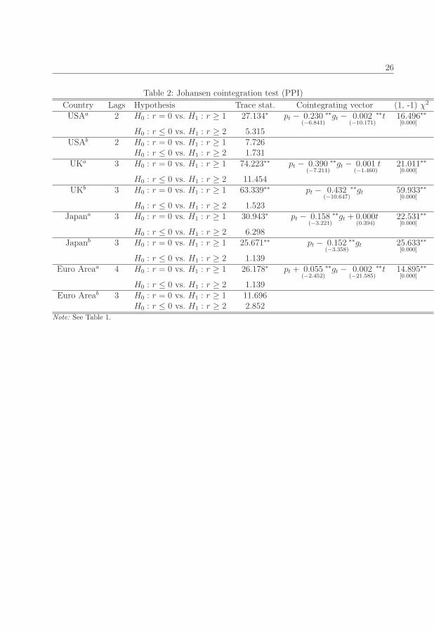
The results of the trace test developed by Johansen (1988, 1991) are presented in Table 1

and 2 for the CPI’s and PPI’s, respectively. For each price measure, the null of no coin-

tegration can significantly be rejected while the null of one cointegrating relation (r = 1)

14Among others Francis and Owyang (2005) followed the same methodology.

13

cannot.15 Merely in two cases the null of no cointegration cannot be rejected: Those are the

PPI configurations for the USA and the Euro Area both with an unrestricted constant. In

both cases, we do not estimate the cointegration coefficients. These findings may be simply

explained by the significance of the trend within the cointegration space in the first specifica-

tion. Conditional on r = 1, the coefficients of the cointegrating relation between the general

price level and the price for gold have been estimated for all other settings and are reported

in Tables 1 and 2 as well.

Table 1 and 2 about here

According to Wang et al. (2011) the long-run relationship between the price level and the

gold price should be proportional if gold is able to fully hedge inflation. The cointegration

vectors have been normalized on the CPI and PPI, respectively, and in each case the gold

coefficients have the expected sign; however they are less than unity in magnitude. As can

be seen in Table 1 and 2, respectively, most of the gold coefficients are highly significant.

The only exception is the restricted trend specification for the Euro Area where the CPI

is used as the price level. In that cointegrating relation, the gold price is not significant,

thus we do not estimate the time-varying adjustment coefficients in this case. Overall, the

gold coefficients range from 0.23 to 0.43 in case of the USA, from 0.35 to 0.45 for the UK

and from 0.15 to 0.23 in case of Japan. For the Euro Area, the significant coefficients turn

out to be 0.196 (CPI) and 0.055 (PPI). Although we still have to consider the time-varying

adjustment coefficients it seems that gold is only partially able to hedge future inflation in

the long-run and this ability is stronger for the USA and the UK compared to Japan and

the Euro Area. The findings for Japan are in line with the outcome of Wang et al. (2011)

and may, for instance, be explained by the inclusion of the deflation experience since the

nineties where gold prices may have lost their function as a leading indicator. In case of the

Eurozone, our findings can possibly be attributed to different inflation expectations across

countries prior to the introduction of the Euro. Turning to the magnitudes of the long-run

coefficients, the latter hardly differ between the CPI and PPI configuration for the UK. Ho-

wever, the CPI coefficients are always higher for Japan and the United States compared to

the PPI configurations. The highest coefficient for the Euro Area is also observed for the CPI

set-up. Hence, the long-run hedge against inflation provided by gold tends to be stronger for

consumer prices. Overall, the general findings are remarkable robust since the verification of

a long-run relationship is always independent of the chosen price measure (PPI or CPI) and

15The test statistic of the corresponding likelihood test, the so-called trace test, is given by trace(r) =

−TK∑

i=r+1

log(1 − λi). Under the null of K − r unit roots λi, i = r + 1, . . . ,K, should behave like ran-

dom walks and the test statistic should be small. Starting with the hypothesis of full rank, the rank isdetermined by using a top-bottom procedure until the null cannot be rejected (Juselius, 2006).

14

only differs in two cases with respect to the deterministic components incorporated into the

model.

A test of the proportionality restriction based on a likelihood ratio (LR) procedure suggested

by Juselius (2006) confirms the inability of gold to provide a full hedge against inflation. The

test statistics which are also given in Tables 1 and 2 confirm our results since the restriction

is clearly rejected for each country.16

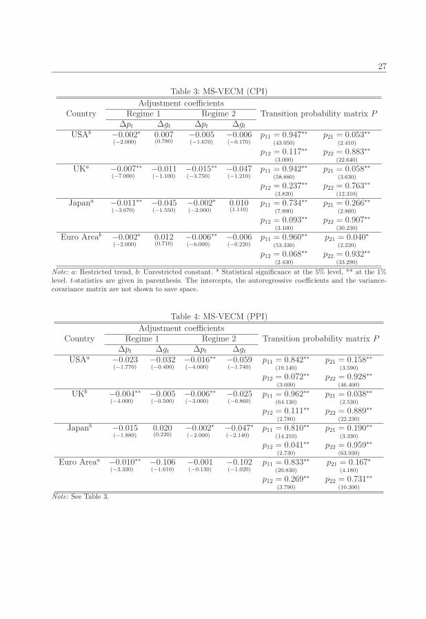
As a next step the MS-VECM representation given in equation (1) has been estimated for

each country while we allowed for two states and let each parameter switch, the intercept

terms, the autoregressive components, the variance-covariance matrix of the errors and espe-

cially the adjustment parameters to deviations from the mentioned long-run relations.17 As

previously mentioned, the time-varying adjustment coefficients are able to discriminate bet-

ween periods with and without hedging functions since gold is not able to shield a portfolio

with respect to future price movements if prices do not adjust to the long-run relation.

To estimate the MS-VECM for each setting we apply the cointegrating relations with a re-

stricted trend given in Table 1 and 2 (a), respectively, as long as the trend is significant,

otherwise we use the specification with an unrestricted constant (b) following Juselius (2006).

In some cases it appeared tractable to restrict the autoregressive components not to switch

between regimes according to Francis and Owyang (2005). Tables 3 and 4 provide the esti-

mated adjustment parameters to short-run deviations of the long-run relationships given

in Tables 1 and 2 that vary across regimes and Tables 3 and 4 also report the transition

probabilities between states.

Table 3 and 4 about here

As can be seen in Table 3 and 4 for each country the CPI and PPI, respectively, adjusts

statistically significant to deviations from the stable long-run equilibrium. Thus, it becomes

evident that the general price level reacts to variations of the price for gold that let the price

level drift apart from its equilibrium path. Overall, a reasonable conclusion is that gold price

movements mirror changes of inflationary expectations and hence, signal the formation of

future inflation. Thus, gold can effectively be used to hedge against inflation. Furthermore, it

16Additionally, we applied LR tests of exclusion for each setting which confirm the robustness of our esti-mated long-run relations. To conserve space we do not report the corresponding test statistics, howeverthese could be provided upon request.

17We have also considered more than two states, but that did not seem to be feasible in our framework sinceat least one state did not had enough periods identified to estimate the regime switching parametersconfidently.

15

is obvious that the price level adjusts to short-run errors either in both regimes with different

speed of adjustment as in case of the UK, Japan (CPI), and the Euro Area (CPI) or just in

one regime as in case of the USA, Japan (PPI), and the Euro Area (PPI). Hence, the ability

to hedge according to the long-run coefficients is not continuously in the latter cases and

differs for the former settings. For instance, in case of the UK the CPI corrects deviations

from the long-run relation between the CPI and the price for gold by 0.7 per cent per month

in the first regime and twice as fast in the second regime. Overall, it seems that the nonlinear

structure of the dynamics between the general price level and the gold price is adequately

accounted for by our state-dependent approach.

Moreover, the transition probabilities are highly significant for each country and show that

regimes are generally persistent in each case since the probabilities of staying in a given state

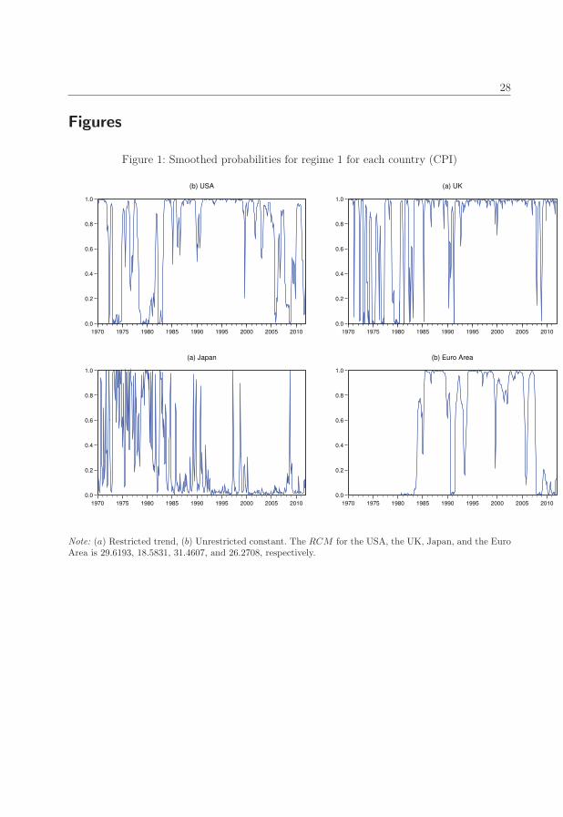
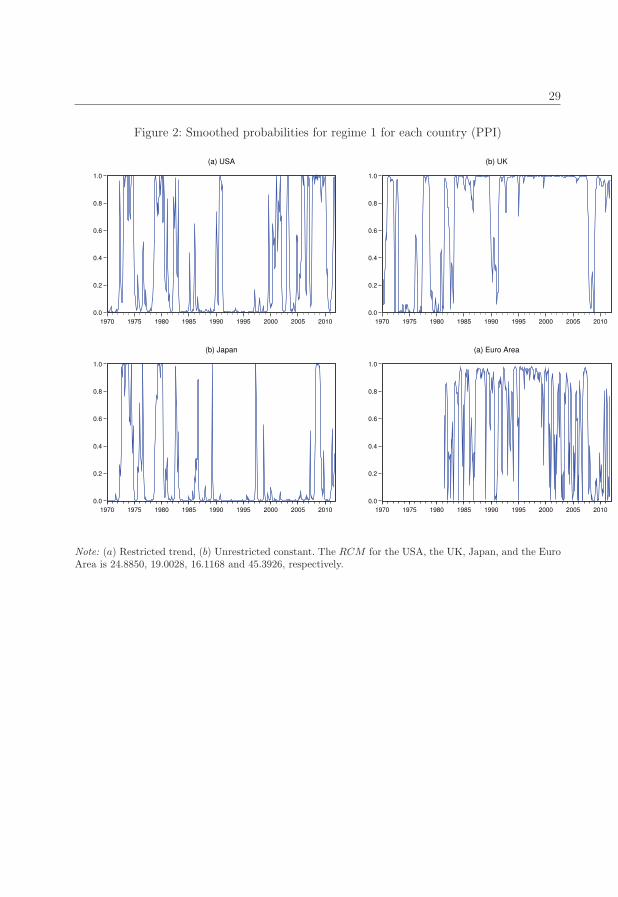
a relatively large. The series of smoothed probabilities also achieved by the Gibbs sampling

technique and shown in Figure 1 and 2, respectively, illustrate the reconstructed incidences

of the first regime over the whole sample period by inferring the probabilities of the occur-

rence of the unobserved states conditional on the available information in the whole dataset

which allows a ’real time’ classification of the regime switches (Krolzig, 2003). For regime

classification Hamilton (1989) suggested the use of a probability of 0.5.

A graphical inspection of Figures 1 and 2 shows that a switching between both regimes

frequently occurs at the beginning of the sample after the breakdown of Bretton Woods.

Although a definite interpretation of the economic circumstances related to specific regimes

is a notorious difficult task, one regime approximately seems to account for times of turbu-

lences such as until the mid-80’s or during the recent global financial crisis while the other

corresponds to ’normal times’ which are unaffected by major shocks due to historical events.

For the United States, the probability for regime 1 for the CPI measure and regime 2 for the

PPI measure is much higher between 1985 and 2000, a time period which may be labeled

as ’normal times’. In both cases, prices only adjust in the latter mentioned regime. The

findings for Japan suggest that the second regime is more probable during the nineties, a

period during which the Japanese economy suffered from deflation and stagnation. However,

the adjustment seems to be faster during the other regime although the PPI adjustment

coefficient for the first regime is a borderline case in terms of significance. As previously

mentioned, the price for gold may exhibit less information with respect to future price mo-

vements in a deflationary environment. For the UK, the first regime where adjustment is

(slightly) weaker seems to correspond to ’normal times’. The regime pattern for the Euro

Area is less clear-cut since the seventies as a period of turbulences are not included. Thus,

16

the adjustment pattern of the price level to the gold price depends on whether economic

turbulences occur or not. However, an unambiguous time pattern across countries cannot be

observed, mirroring that each economy has its own characteristics.

Figure 1 and 2 about here

Finally, the regime classification measure (RCM) suggested by Ang and Bekaert (2002)

indicates a good fit of our MS-VECM for each country (see Notes of Figure 1 and 2). The

RCM statistic is computed as follows

RCM(M) = 100M2 1

Tj

Tj∑

t=1

M∏

j=1

pj,t, (3)

where pj,t denotes the smoothed probability for regime j and provides a degree of accuracy

with which a model identifies regime switching behavior over the entire sample period or

a particular sub sample period. The regime variable is Bernoulli distributed and thus, the

RCM corresponds to a sample estimator of its variance. It takes values between 0 and

100, with 0 representing a perfect regime classification performance and 100 denoting that

the model fails to exhibit any information about the regime-dependence. For most of the

countries the value of the RCM statistic is fairly low (always below 50) and thus, one could

conclude that our models are adequately specified.

5 Conclusion

This study has analyzed whether gold provides the ability of hedging inflation for four major

economies, namely the USA, the UK, the Euro Area, and Japan, by allowing for nonlinearity

and discriminating between long-run and time-varying short-run dynamics. To the best of

our knowledge our study is the first to consider a VECM approach with Markovian shifts

in the adjustment parameters to short-run deviations from the long-run relations in this

context. Our main findings are threefold: First, we show that gold is partially able to hedge

future inflation in the long-run. This ability tends to be stronger for consumer prices in

general as well as for the USA and the UK compared to Japan and the Euro Area. Secondly,

the adjustment of the general price level seems to be appropriately characterized by regime-

dependence. Finally, we display that one regime may account for times of turbulences and

the other for ’normal times’ which are unaffected by major shocks. Thus, the different ad-

justment pattern of the price level may depend on the occurrence of economic turbulences.

Due to this finding, the price for gold should be considered when aiming to appropriately

17

forecast the inflation rate.18

From an investor’s point of view, the effectiveness of gold as an inflation hedge crucially

depends on the time horizon. Over the very long-run, gold is useful as a partial hedge since a

cointegrating relationship prevails. However, during some periods where no price adjustment

is observed, gold is not able to shield a portfolio. This may be illustrated by a simple example

of an investor who buys gold at the beginning of a period with no adjustment and sells at

the end of the corresponding period.

However, since each economy has its own characteristics, we are unable to detect an overall

unambiguous time pattern across countries. An interesting topic for further research may be

the analysis of gold as a hedge or ’safe haven’ with respect to stock markets in a time-varying

framework. The possibility to apply daily data in such an analysis may contribute to further

insights with respect to the importance of gold for portfolio investors over the very short-

run. Another appealing question is how does gold perform against other potential inflation

hedges such as stocks, bonds, real estate, or other commodities in our framework.19

References

Adrangi, B., A. Chatrath and K. Raffiee (2003): Economic Activity, Inflation, and

Hedging: The Case of Gold and Silver Investments. The Journal of Wealth Manage-

ment, 6(2), 60-77.

Aggarwal, R. (1992): Gold Markets. In: Newman, P., Milgate, M., Eatwell, J. (Eds.) The

New Palgrave Dictionary of Money and Finance (Vol. 2). Basingstoke: Macmillan,

257-258.

Aizenman, J. and K. Inoue (2012): Central Banks and Gold Puzzles. NBER Working

Paper, No. 17894.

Albert, J. and S. Chib (1993): Bayesian Analysis of Binary and Polychotomous Re-

sponse Data. Journal of the American Statistical Association, 88(422), 669-679.

18For instance, the gold price could be incorporated into an inflation forecast framework based on the p-starapproach proposed by Czudaj (2011) among others.

19This question has already been tackled in the course of a correlation study by Spierdijk and Umar (2010)which is based on a standard VAR framework. As hedging measures Spierdijk and Umar (2010) applythe Pearson correlation coefficient, the Fisher coefficient in the Fama and Schwert (1977) regression,the hedge ratio proposed by Schotman and Schweizer (2000), the hedging capacity suggested by Bodie(1976) as well as the associated cost of hedging. Their analysis indicates that energy commodities andnon-precious metals provide the best inflation hedges.

18

Ang, A. and G. Bekaert (2002): Regime Switches in Interest Rates. Journal of Business

& Economic Statistics, 20(2), 163-182.

Ariovich, G. (1983): The Impact of Political Tension on the Price of Gold. Journal for

Studies in Economics and Econometrics, 16(1), 17-37.

Baker, S.A. and R.C. van Tassel (1985): Forecasting the Price of Gold: A Fundamen-

talist Approach. Atlantic Economic Journal, 13(4), 43-51.

Balke, N.S. and T.B. Fomby (1997): Threshold Cointegration. International Economic

Review, 38(3), 627-645.

Basu, S. and M.L. Clouse (1993): A Comparative Analysis of Gold Market Efficiency

Using Derivative Market Information. Resources Policy, 19(3), 217-224.

Baur, D.G. and B.M. Lucey (2010): Is Gold a Hedge or a Safe Haven? An Analysis of

Stocks, Bonds and Gold. The Financial Review, 45(2), 217-229.

Baur, D.G. and T.K. McDermott (2010): Is Gold a Safe Haven? International Evi-

dence. Journal of Banking & Finance, 34(8), 1886-1898.

Bialkowski, J.T., M.T. Bohl, P.M. Stephan and T.P. Wisniewski (2011): Is

There a Speculative Bubble in the Price of Gold? Available from SSRN:

http://ssrn.com/abstract=1718106.

Blose, L.E. (2010): Gold Prices, Cost of Carry, and Expected Inflation. Journal of Eco-

nomics and Business, 62(1), 35-47.

Bodie, Z. (1976): Common Stocks as a Hedge against Inflation. Journal of Finance, 31(2),

459-470.

Capie, F., T.C. Mills and G. Wood (2005): Gold as a Hedge Against the Dollar.

Journal of International Financial Markets, Institutions and Money, 15(4), 343-352.

Cecchetti, S.G., R.S. Chu and C. Steindel (2000): The Unreliability of Inflation

Indicators. Current Issues in Economics & Finance, 6(4), 1-6.

Chappell, D. and K. Dowd (1997): A Simple Model of the Gold Standard. Journal of

Money, Credit and Banking, 29(1), 94-105.

Chua, J., G. Stick and R. Woodward (1990): Diversifying with Gold Stocks. Financial

Analysts Journal, 46(4), 76-79.

19

Ciner, C. (2001): On the Long Run Relationship between Gold and Silver: A Note. Global

Finance Journal, 12(2), 299-303.

Ciner, C., C. Gurdgiev and B.M. Lucey (2010): Hedges and Safe Havens - An Ex-

amination of Stocks, Bonds, Oil, Gold and the Dollar. IIIS Discussion Paper, No. 337.

Czudaj, R. (2011): P-star in Times of Crisis - Forecasting Inflation for the Euro Area.

Economic Systems, 35(3), 390-407.

Dempster, A.P., N.M. Laird and D.B. Rubin (1977): Maximum Likelihood Esti-

mation from Incomplete Data via the EM Algorithm. Journal of the Royal Statistical

Society, 39 (Series B), 1-38.

Diba, B.T. and H.I. Grossman (1984): Rational Bubbles in the Price of Gold. NBER

Working Paper, No. 1300.

Dickey, D. and W.A. Fuller (1979): Distribution of the Estimates for Autoregressive

Time Series with a Unit Root. Journal of the American Statistical Association, 74(366),

427-431.

Dooley, M.P., P. Isard and M.P. Taylor (1995): Exchange Rates, Country-Specific

Shocks and Gold. Applied Financial Economics, 5(3), 121-129.

Enders, W. and P. Siklos (2001): Cointegration and Threshold Adjustment. Journal

of Business & Economic Statistics, 19(2), 166-176.

Engle, R.F. and C.W.J. Granger (1987): Cointegration and Error Correction: Repre-

sentation, Estimation and Testing. Econometrica, 55(2), 251-276.

Fama, E.F. and G.W. Schwert (1977): Asset Returns and Inflation. Journal of Finan-

cial Economics, 5(2), 115-146.

Filardo, A.J. (1994): Business-Cycle Phases and Their Transitional Dynamics. Journal

of Business & Economic Statistics, 12(4), 299-308.

Francis, N. and M.T. Owyang (2005): Monetary Policy in a Markov-Switching Vector

Error-Correction Model. Journal of Business & Economic Statistics, 23(3), 305-313.

Garner, C.A. (1995): How Useful Are Leading Indicators of Inflation? Federal Reserve

Bank of Kansas City, Economic Review, Second Quarter, 5-18.

20

Geman, S., and D. Geman (1984): Stochastic Relaxation, Gibbs Distributions and the

Bayesian Restoration of Images. IEEE Transactions on Pattern Analysis and Machine

Intelligence, 6(6), 721-741.

Gosh, D., E.J. Levin, P. Macmillan and R.E. Wright (2004): Gold as an Inflation

Hedge? Studies in Economics and Finance, 22(1), 1-25.

Hamilton, J.D. (1989): A New Approach to the Economic Analysis of Nonstationary

Time Series and the Business Cycle. Econometrica, 57(2), 357-384.

Hamilton, J.D. (1993): Estimation, Inference and Forecasting of Time Series Subject to

Changes in Regime. In: Maddala, G.S., Rao, C.R., Vinod, H.D. (Eds.), Handbook of

Econometrics (Vol. 4), Amsterdam: Elsevier.

Hansen, B.E. and B. Seo (2002): Testing for Two-Regime Threshold Cointegration in

Vector Error-Correction Models. Journal of Econometrics, 110(2), 293-318.

Harmston, S. (1998): Gold as a Store of Value. World Gold Council, Research Study, No.

22.

Ho, Y.K. (1985): Test of the Incrementally Efficient Market Hypothesis for the London

Gold Market. Economics Letters, 19(1), 67-70.

Ihle, R. and S. v. Cramon-Taubadel (2008): A Comparison of Threshold Cointe-

gration and Markov-Switching Vector Error Correction Models in Price Transmission

Analysis. Proceedings of the NCCC-134 Conference on Applied Commodity Price Ana-

lysis, Forecasting, and Market Risk Management, St. Louis, MO.

Jaffe, J. (1989): Gold and Gold Stocks as Investments for Institutional Portfolios. Finan-

cial Analysts Journal, 45(2), 53-59.

Johansen, S. (1988): Statistical Analysis of Cointegration Vectors. Journal of Economic

Dynamics and Control, 12(2-3), 231-254.

Johansen, S. (1991): Estimation and Hypothesis Testing of Cointegrated Vectors in Gaus-

sian Vector Autoregressive Models. Econometrica, 59(6), 1551-1580.

Juselius, K. and R. MacDonald (2004): International Parity Relationships between

the USA and Japan. Japan and the World Economy, 16(1), 17-34.

Juselius, K. (2006): The Cointegrated VAR Model: Econometric Methodology and Macro-

economic Applications. Oxford: Oxford University Press.

21

Kim, C.-J. and C.R. Nelson (1999): State-Space Models with Regime Switching. Cam-

bridge: MIT Press.

Kolluri, B.R. (1981): Gold as a Hedge Against Inflation: An Empirical Investigation.

The Quarterly Review of Economics and Business, 21(4), 13-24.

Koutsoyiannis, A. (1983): A Short-Run Pricing Model for a Speculative Asset, Tested

with Data from the Gold Bullion Market. Applied Economics, 15(5), 563-581.

Krolzig, H.-M. (1997): Markov-Switching Vector Autoregressions: Modelling, Statistical

Inference, and Application to Business Cycle Analysis, Lecture Notes in Economics

and Mathematical Systems (Vol. 454), New York: Springer.

Krolzig, H.-M. (2003): Constructing Turning Point Chronologies with Markov-Switching

Vector Autoregressive Models: The Euro-Zone Business Cycle. In: Eurostat (ed.), Pro-

ceedings on Modern Tools for Business Cycle Analysis. Monography in Official Stati-

stics.

Kyrtsou, C. and W. Labys (2006): Evidence for Chaotic Dependence between U.S.

Inflation and Commodity Prices. Journal of Macroeconomics, 28(1), 256-266.

Laurent, R.D. (1994): Is There a Role for Gold in Monetary Policy? Federal Reserve

Bank of Chicago, Economic Perspectives, March, 2-14.

Lawrence, C. (2003): Why is Gold Different from Other Assets? An Empirical Investi-

gation. London: World Gold Council.

Levin, E.R. and R.E. Wright (2006): Short-Run and Long-Run Determinants of the

Price of Gold. World Gold Council, Research Study, No. 32.

Lo, M.C. and E. Zivot (2001): Threshold Cointegration and Nonlinear Adjustment to

the Law of One Price. Macroeconomic Dynamics, 5(4), 533-576.

Lucey, B.M., E. Tully and V. Poti (2006): International Portfolio Formation, Skew-

ness and the Role of Gold. Frontiers in Finance and Economics, 3(1), 1-17.

MacKinnon, J.G., A.A. Haug, and L. Michelis (1999): Numerical Distribution Func-

tions of Likelihood Ratio Tests for Cointegration. Journal of Applied Econometrics,

14(5), 563-577.

Mahdavi, S. and S. Zhou (1997): Gold and Commodity Prices as Leading Indicators

of Inflation: Tests of Long-Run Relationship and Predictive Performance. Journal of

Economics and Business, 49(5), 475-489.

22

McCown, J.R. and J.R. Zimmerman (2006): Is Gold a Zero-Beta Asset? Analysis of

the Investment Potential of Precious Metals. Available from SSRN:

http://ssrn.com/abstract=920496.

McCulloch, R.E. and R.S. Tsay (1994): Statistical Analysis of Economic Time Series

via Markov Switching Models. Journal of Time Series Analysis, 15(5), 523-539.

Michaud, R., R. Michaud and K. Pulvermacher (2006): Gold as Strategic Asset.

London: World Gold Council.

Moore, G. (1990): Gold Prices and a Leading Index of Inflation. Challenge, 33(4), 52-56.

Ng, S. and P. Perron (2001): Lag Length Selection and the Construction of Unit Root

Tests with Good Size and Power. Econometrica, 69(6), 1519-1554.

Perron, P. (1989): The Great Crash, the Oil Price Shock, and the Unit Root Hypothesis.

Econometrica, 57(6), 1361-1401.

Pindyck, R.S. (1993): The Present Value Model of Rational Commodity Pricing. The

Economic Journal, 103(418), 511-530.

Rahbek, A., E. Hansen and J.G. Dennis (2002): ARCH Innovations and Their Impact

on Cointegration Rank Testing. Department of Theoretical Statistics, University of

Copenhagen, Centre for Analytical Finance, Working Paper, No. 22.

Saikkonen, P. (1992): Estimation and Testing of Cointegrated Systems by an Autore-

gressive Approximation. Econometric Theory, 8(1), 1-27.

Saikkonen, P. and R. Luukkonen (1997): Testing Cointegration in Infinite Order

Vector Autoregressive Processes. Journal of Econometrics, 81(1), 93-126.

Saikkonen, P. and H. Lutkepohl (2000a): Testing for the Cointegrating Rank of a

VAR Process with an Intercept. Econometric Theory, 16(3), 373-406.

Saikkonen, P. and H. Lutkepohl (2000b): Testing for the Cointegrating Rank of a

VAR Process with Structural Shifts. Journal of Business & Economic Statistics, 18(4),

451-464.

Saikkonen, P. and H. Lutkepohl (2000c): Trend Adjustment Prior to Testing for

the Cointegrating Rank of a Vector Autoregressive Process. Journal of Time Series

Analysis, 21(4), 435-456.

23

Sarno, L. and G. Valente (2006): Deviations from Purchasing Power Parity under

Different Exchange Rate Regimes: Do They Revert and, if so, How? Journal of Banking

& Finance, 30(11), 3147-3169.

Schotman, P.C. and M. Schweitzer (2000): Horizon Sensitivity of the Inflation Hedge

of Stocks. Journal of Empirical Finance, 7(3), 301-315.

Sherman, E. (1982): New Gold Model Explains Variations. Commodity Journal, 17, 16-20.

Sherman, E. (1983): A Gold Pricing Model. Journal of Portfolio Management, 9(3), 68-70.

Sherman, E. (1986): Gold Investment: Theory and Application. New York: Prentice Hall.

Sjaastad, L.A. and F. Scacciallani (1996): The Price of Gold and the Exchange

Rate. Journal of International Money and Finance, 15(6), 879-897.

Smith, G. (2002): Tests of the Random Walk Hypothesis for London Gold Prices. Applied

Economics Letters, 9(10), 671-674.

Solt, M.E. and P.J. Swanson (1981): On the Efficiency of the Markets for Gold and

Silver. Journal of Business, 54(3), 453-478.

Spierdijk, L. and Z. Umar (2010): Are Commodities a Good Hedge against Inflation?

A Comparative Approach. Netspar Discussion Paper, No. 11/2010-078.

Tkacz, G. (2007): Gold Prices and Inflation. Bank of Canada, Research Department, 1-29.

Tschoegl, A.E. (1980): Efficiency in the Gold Market. Journal of Banking & Finance,

4(4), 371-379.

Tully, E. and B.M. Lucey (2007): A Power GARCH Examination of the Gold Market.

Research in International Business and Finance, 21(2), 316-325.

Wang, K.-M. and Y.-M. Lee (2011): The Yen for Gold. Resources Policy, 36(1), 39-48.

Wang, K.-M., Y.-M. Lee and T.-B. Nguyen Thi (2011): Time and Place Where Gold

Acts as an Inflation Hedge: An Application of Long-Run and Short-Run Threshold

Model. Economic Modelling, 28(3), 806-819.

Worthington, A.C. and M. Pahlavani (2007): Gold Investment as an Inflationa-

ry Hedge: Cointegration Evidence with Allowance for Endogenous Structural Breaks.

Applied Financial Economics Letters, 3(4), 259-262.

24

Zivot, E. and D.W.K. Andrews (1992): Further Evidence on the Great Crash, the Oil

Price Shock, and the Unit Root Hypothesis. Journal of Business & Economic Statistics,

10(3), 251-270.

25

Tables

Table 1: Johansen cointegration test (CPI)

Country Lags Hypothesis Trace stat. Cointegrating vector (1, -1) χ2

USAa 2 H0 : r = 0 vs. H1 : r ≥ 1 62.133∗∗ pt − 0.408(−5.594)

∗∗gt − 0.000(−0.532)

t 41.090[0.000]

∗∗

H0 : r ≤ 0 vs. H1 : r ≥ 2 13.548∗

USAb 2 H0 : r = 0 vs. H1 : r ≥ 1 51.025∗∗ pt − 0.433(−8.757)

∗∗gt 41.053[0.000]

∗∗

H0 : r ≤ 0 vs. H1 : r ≥ 2 2.478UKa 4 H0 : r = 0 vs. H1 : r ≥ 1 84.096∗∗ pt − 0.359

(−7.648)

∗∗gt − 0.001(−2.729)

∗∗t 28.105[0.000]

∗∗

H0 : r ≤ 0 vs. H1 : r ≥ 2 11.323UKb 4 H0 : r = 0 vs. H1 : r ≥ 1 49.252∗∗ pt − 0.455

(−10.377)

∗∗gt 66.393[0.000]

∗∗

H0 : r ≤ 0 vs. H1 : r ≥ 2 2.011Japana 2 H0 : r = 0 vs. H1 : r ≥ 1 129.233∗∗ pt − 0.231

(−3.570)

∗∗gt − 0.001(−4.934)

∗∗t 17.016[0.000]

∗∗

H0 : r ≤ 0 vs. H1 : r ≥ 2 7.636Japanb 2 H0 : r = 0 vs. H1 : r ≥ 1 112.270∗∗ pt − 0.177

(−4.290)

∗∗gt 100.656[0.000]

∗∗

H0 : r ≤ 0 vs. H1 : r ≥ 2 1.107Euro Areaa 2 H0 : r = 0 vs. H1 : r ≥ 1 114.175∗∗ pt + 0.006

(0.329)gt − 0.002

(−22.099)

∗∗t 48.848[0.000]

∗∗

H0 : r ≤ 0 vs. H1 : r ≥ 2 7.322Euro Areab 4 H0 : r = 0 vs. H1 : r ≥ 1 36.976∗∗ pt − 0.196

(−2.610)

∗∗gt 25.477[0.000]

∗∗

H0 : r ≤ 0 vs. H1 : r ≥ 2 2.589

Note: a: Restricted trend, b: Unrestricted constant. * Statistical significance at the 5% level, ** at the 1%level. The t-statistics of the cointegration coefficients are given in parenthesis and the p-values of the LRtest of the restricted model are reported in brackets. In case of insignificance the trend is deleted from thecointegrating space, allowing for a linear trend in the data, but not in the cointegrating equation. Criticalvalues for testing (i) H0 : r = 0 and (ii) H0 : r ≤ 1 are taken from MacKinnon et al. (1999): (a) 5% (i)25.731 and (ii) 12.448, 1% (i) 31.153 and (ii) 16.553, (b) 5% (i) 15.408 and (ii) 3.841, 1% (i) 19.937 and (ii)6.634, respectively.

26

Table 2: Johansen cointegration test (PPI)

Country Lags Hypothesis Trace stat. Cointegrating vector (1, -1) χ2

USAa 2 H0 : r = 0 vs. H1 : r ≥ 1 27.134∗ pt − 0.230(−6.841)

∗∗gt − 0.002(−10.171)

∗∗t 16.496[0.000]

∗∗

H0 : r ≤ 0 vs. H1 : r ≥ 2 5.315USAb 2 H0 : r = 0 vs. H1 : r ≥ 1 7.726

H0 : r ≤ 0 vs. H1 : r ≥ 2 1.731UKa 3 H0 : r = 0 vs. H1 : r ≥ 1 74.223∗∗ pt − 0.390

(−7.211)

∗∗gt − 0.001(−1.460)

t 21.011[0.000]

∗∗

H0 : r ≤ 0 vs. H1 : r ≥ 2 11.454UKb 3 H0 : r = 0 vs. H1 : r ≥ 1 63.339∗∗ pt − 0.432

(−10.647)

∗∗gt 59.933[0.000]

∗∗

H0 : r ≤ 0 vs. H1 : r ≥ 2 1.523Japana 3 H0 : r = 0 vs. H1 : r ≥ 1 30.943∗ pt − 0.158

(−3.221)

∗∗gt + 0.000(0.394)

t 22.531[0.000]

∗∗

H0 : r ≤ 0 vs. H1 : r ≥ 2 6.298Japanb 3 H0 : r = 0 vs. H1 : r ≥ 1 25.671∗∗ pt − 0.152

(−3.358)

∗∗gt 25.633[0.000]

∗∗

H0 : r ≤ 0 vs. H1 : r ≥ 2 1.139Euro Areaa 4 H0 : r = 0 vs. H1 : r ≥ 1 26.178∗ pt + 0.055

(−2.452)

∗∗gt − 0.002(−21.585)

∗∗t 14.895[0.000]

∗∗

H0 : r ≤ 0 vs. H1 : r ≥ 2 1.139Euro Areab 3 H0 : r = 0 vs. H1 : r ≥ 1 11.696

H0 : r ≤ 0 vs. H1 : r ≥ 2 2.852Note: See Table 1.

27

Table 3: MS-VECM (CPI)

Adjustment coefficientsCountry Regime 1 Regime 2 Transition probability matrix P

Δpt Δgt Δpt ΔgtUSAb −0.002

(−2.000)

∗ 0.007(0.780)

−0.005(−1.670)

−0.006(−0.170)

p11 = 0.947∗∗(43.050)

p21 = 0.053∗∗(2.410)

p12 = 0.117∗∗(3.000)

p22 = 0.883∗∗(22.640)

UKa −0.007(−7.000)

∗∗ −0.011(−1.100)

−0.015(−3.750)

∗∗ −0.047(−1.210)

p11 = 0.942∗∗(58.880)

p21 = 0.058∗∗(3.630)

p12 = 0.237∗∗(3.820)

p22 = 0.763∗∗(12.310)

Japana −0.011(−3.670)

∗∗ −0.045(−1.550)

−0.002(−2.000)

∗ 0.010(1.110)

p11 = 0.734∗∗(7.890)

p21 = 0.266∗∗(2.860)

p12 = 0.093∗∗(3.100)

p22 = 0.907∗∗(30.230)

Euro Areab −0.002(−2.000)

∗ 0.012(0.710)

−0.006(−6.000)

∗∗ −0.006(−0.220)

p11 = 0.960∗∗(53.330)

p21 = 0.040∗(2.220)

p12 = 0.068∗∗(2.430)

p22 = 0.932∗∗(33.290)

Note: a: Restricted trend, b: Unrestricted constant. * Statistical significance at the 5% level, ** at the 1%level. t-statistics are given in parenthesis. The intercepts, the autoregressive coefficients and the variance-covariance matrix are not shown to save space.

Table 4: MS-VECM (PPI)

Adjustment coefficientsCountry Regime 1 Regime 2 Transition probability matrix P

Δpt Δgt Δpt ΔgtUSAa −0.023

(−1.770)−0.032(−0.400)

−0.016(−4.000)

∗∗ −0.059(−1.740)

p11 = 0.842∗∗(19.140)

p21 = 0.158∗∗(3.590)

p12 = 0.072∗∗(3.600)

p22 = 0.928∗∗(46.400)

UKb −0.004(−4.000)

∗∗ −0.005(−0.500)

−0.006(−3.000)

∗∗ −0.025(−0.860)

p11 = 0.962∗∗(64.130)

p21 = 0.038∗∗(2.530)

p12 = 0.111∗∗(2.780)

p22 = 0.889∗∗(22.230)

Japanb −0.015(−1.880)

0.020(0.220)

−0.002(−2.000)

∗ −0.047(−2.140)

∗ p11 = 0.810∗∗(14.210)

p21 = 0.190∗∗(3.330)

p12 = 0.041∗∗(2.730)

p22 = 0.959∗∗(63.930)

Euro Areaa −0.010(−3.330)

∗∗ −0.106(−1.610)

−0.001(−0.130)

−0.102(−1.020)

p11 = 0.833∗∗(20.830)

p21 = 0.167∗(4.180)

p12 = 0.269∗∗(3.790)

p22 = 0.731∗∗(10.300)

Note: See Table 3.

28

Figures

Figure 1: Smoothed probabilities for regime 1 for each country (CPI)

0.0

0.2

0.4

0.6

0.8

1.0

1970 1975 1980 1985 1990 1995 2000 2005 2010

(b) USA

0.0

0.2

0.4

0.6

0.8

1.0

1970 1975 1980 1985 1990 1995 2000 2005 2010

(a) UK

0.0

0.2

0.4

0.6

0.8

1.0

1970 1975 1980 1985 1990 1995 2000 2005 2010

(a) Japan

0.0

0.2

0.4

0.6

0.8

1.0

1970 1975 1980 1985 1990 1995 2000 2005 2010

(b) Euro Area

Note: (a) Restricted trend, (b) Unrestricted constant. The RCM for the USA, the UK, Japan, and the EuroArea is 29.6193, 18.5831, 31.4607, and 26.2708, respectively.

29

Figure 2: Smoothed probabilities for regime 1 for each country (PPI)

0.0

0.2

0.4

0.6

0.8

1.0

1970 1975 1980 1985 1990 1995 2000 2005 2010

(a) USA

0.0

0.2

0.4

0.6

0.8

1.0

1970 1975 1980 1985 1990 1995 2000 2005 2010

(b) UK

0.0

0.2

0.4

0.6

0.8

1.0

1970 1975 1980 1985 1990 1995 2000 2005 2010

(b) Japan

0.0

0.2

0.4

0.6

0.8

1.0

1970 1975 1980 1985 1990 1995 2000 2005 2010

(a) Euro Area

Note: (a) Restricted trend, (b) Unrestricted constant. The RCM for the USA, the UK, Japan, and the EuroArea is 24.8850, 19.0028, 16.1168 and 45.3926, respectively.