Generalized M-Fluctuation Tests for Parameter Instabilityzeileis/papers/ETSA-2003.pdf ·...
31
Generalized M-Fluctuation Tests for Parameter Instability Achim Zeileis Kurt Hornik
Transcript of Generalized M-Fluctuation Tests for Parameter Instabilityzeileis/papers/ETSA-2003.pdf ·...

Generalized M-Fluctuation Tests forParameter Instability
Achim Zeileis Kurt Hornik
Contents
❆ Model frame
❆ “Philosophy” of generalized fluctuation tests
❆ Generalized M-fluctuation tests
❖ Theoretical M-fluctuation processes
❖ Empirical M-fluctuation processes
❖ Local alternatives
❖ Construction of test statistics
❆ Applications
❖ German M1 money demand
❖ Illegitimate births in Großarl
❆ Software
Model frame
We assume n independent observations
Yi ∼ F (θi) (i = 1, . . . , n).
from distribution F with k-dimensional parameter θi.
Observations are ordered with respect to “time” and can be
vector-valued.
Extension to regression situation and dependent data: later.
Model frame
Null hypothesis:
H0 : θi = θ0 (i = 1, . . . , n).
Alternative:
H1: θi varies over “time” i.

Philosophy
The generalized fluctuation test framework ...
“... includes formal significance tests but its philosophy is basi-
cally that of data analysis as expounded by Tukey. Essentially,
the techniques are designed to bring out departures from con-
stancy in a graphic way instead of parametrizing particular types
of departure in advance and then developing formal significance
tests intended to have high power against these particular alter-
natives.” (Brown, Durbin, Evans, 1975)

Generalized fluctuation tests
❆ empirical fluctuation processes reflect fluctuation in
❖ residuals❖ coefficient estimates❖ M-scores (including OLS or ML scores etc.)
❆ theoretical limiting process is known
❆ choose boundaries which are crossed by the limiting process(or some functional of it) only with a known probability α.
❆ if the empirical fluctuation process crosses the theoreticalboundaries the fluctuation is improbably large ⇒ reject thenull hypothesis.
Generalized M-fluc. processes
Consider a smooth k-dimensional score function ψ(·) with:
E{ψ(Yi, θi)} = 0
and define the covariance matrix
B(θ) = COVθ0{ψ(Y, θ)}.
Generalized M-fluc. tests
A common choice for ψ is the partial derivative of some objective
function Ψ
ψ(y, θ) =∂Ψ(y, θ)
∂θ.
which includes OLS and ML.
In a misspecification context: Quasi-ML, robust M-estimation.
ψ(y, θ) = min(c,max(y − θ,−c)).
Instead of full likelihood use estimating equations, IV, GMM,
GEE.

Theoretical M-fluc. processes
Consider the cumulative score process given by
Wn(t, θ) = n−1/2bntc∑i=1
ψ(Yi, θ).

Theoretical M-fluc. processes
Consider the cumulative score process given by
Wn(t, θ) = n−1/2bntc∑i=1
ψ(Yi, θ).
Under H0 the following functional central limit theorem (FCLT)
holds
B(θ0)−1/2Wn(·, θ0)
d−→ W (·).
Empirical M-fluc. processes
A suitable estimate θn of θ0 is defined by
n∑i=1
ψ(Yi, θn) = 0.
Empirical M-fluc. processes
A suitable estimate θn of θ0 is defined by
n∑i=1
ψ(Yi, θn) = 0.
Under H0 the following FCLT holds
B−1/2n Wn(·, θn) d−→ W0(·),
for some consistent covariance matrix estimate Bn.

Generalized M-fluc. tests
In an empirical sample the empirical M-fluctuation process
efp(t) = B−1/2n Wn(t, θn).
is a k × n array. Can be aggregated to a scalar test statistic by
a functional λ(·)
λ
(efpj
(i
n
)),
where j = 1, . . . , k and i = 1, . . . n.

Generalized M-fluc. tests
λ can usually be split into two components: λtime and λcomp.
Typical choices for λtime: L∞ (absolute maximum), mean, range.
Typical choice for λcomp: L∞, L2.
⇒ can identify component and/or timing of shift. Requires dif-
ferent visualization techniques.
Generalized M-fluc. tests
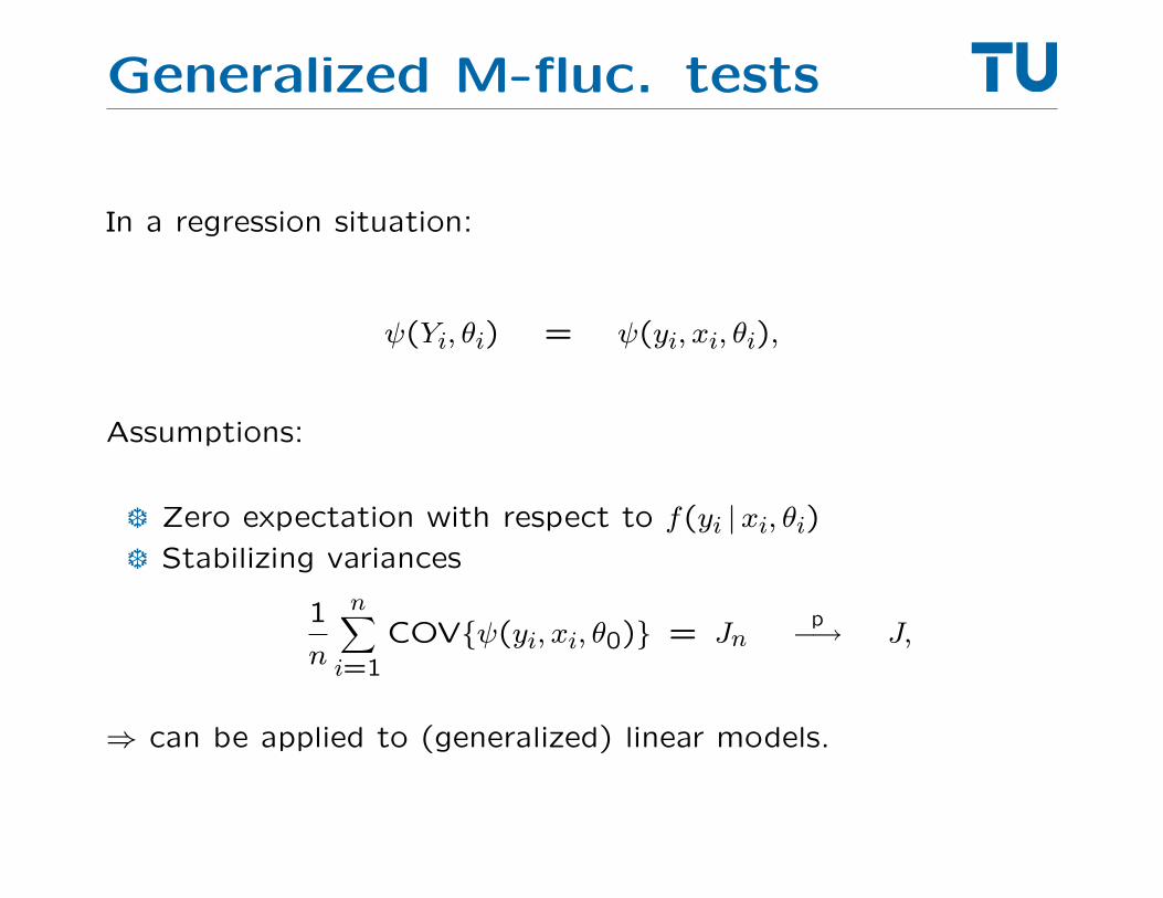
In a regression situation:
ψ(Yi, θi) = ψ(yi, xi, θi),
Assumptions:
❆ Zero expectation with respect to f(yi |xi, θi)❆ Stabilizing variances
1
n
n∑i=1
COV{ψ(yi, xi, θ0)} = Jnp−→ J,
⇒ can be applied to (generalized) linear models.

Generalized M-fluc. tests
Special cases:
❆ Nyblom-Hansen test
❆ OLS-based CUSUM tests
❆ Hjort-Koning tests
❆ robust CUSUM test
❆ . . .
For dependent data:
❆ mean function can usually be estimated consistently,
❆ use HAC covariance matrix estimates.
German M1 money demand
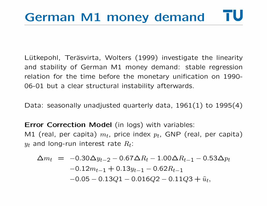
Lutkepohl, Terasvirta, Wolters (1999) investigate the linearity
and stability of German M1 money demand: stable regression
relation for the time before the monetary unification on 1990-
06-01 but a clear structural instability afterwards.
Data: seasonally unadjusted quarterly data, 1961(1) to 1995(4)
Error Correction Model (in logs) with variables:
M1 (real, per capita) mt, price index pt, GNP (real, per capita)
yt and long-run interest rate Rt:
∆mt = −0.30∆yt−2 − 0.67∆Rt − 1.00∆Rt−1 − 0.53∆pt
−0.12mt−1 + 0.13yt−1 − 0.62Rt−1
−0.05− 0.13Q1− 0.016Q2− 0.11Q3 + ut,

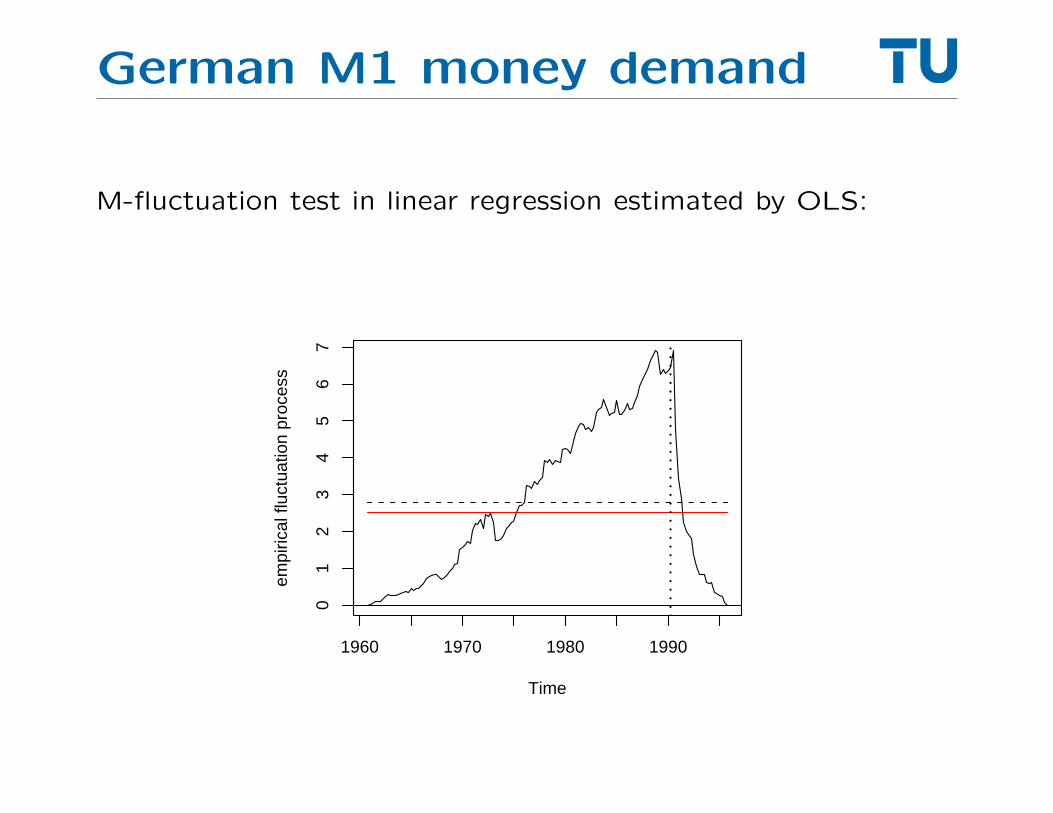
German M1 money demand
M-fluctuation test in linear regression estimated by OLS:
Time
empi
rical
fluc
tuat
ion
proc
ess
1960 1970 1980 1990
01
23
45
67
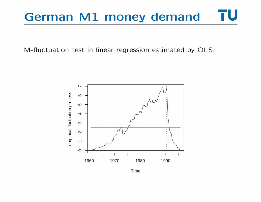
German M1 money demand
M-fluctuation test in linear regression estimated by OLS:
Time
empi
rical
fluc
tuat
ion
proc
ess
1960 1970 1980 1990
01
23
45
67
German M1 money demand
M-fluctuation test in linear regression estimated by OLS:
Time
empi
rical
fluc
tuat
ion
proc
ess
1960 1970 1980 1990
01
23
45
67
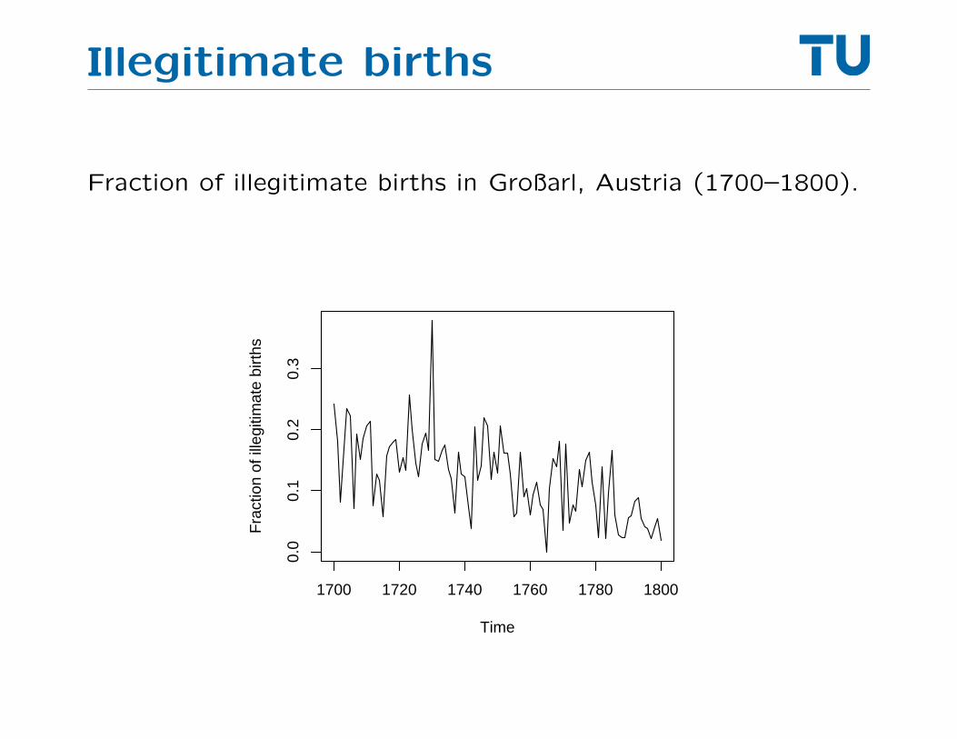
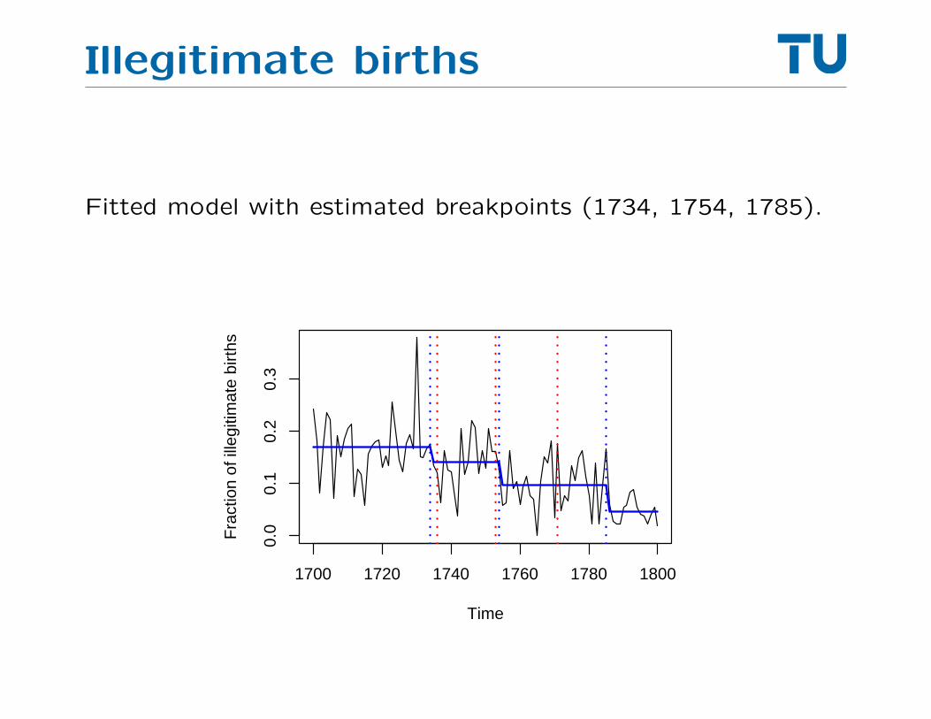
Illegitimate births
Fraction of illegitimate births in Großarl, Austria (1700–1800).
Time
Fra
ctio
n of
ille
gitim
ate
birt
hs
1700 1720 1740 1760 1780 1800
0.0
0.1
0.2
0.3
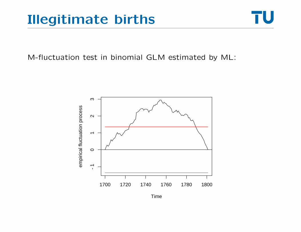
Illegitimate births
M-fluctuation test in binomial GLM estimated by ML:
Time
empi
rical
fluc
tuat
ion
proc
ess
1700 1720 1740 1760 1780 1800
−1
01
23
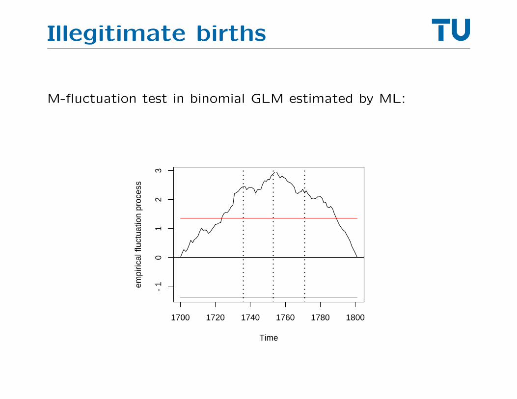
Illegitimate births
M-fluctuation test in binomial GLM estimated by ML:
Time
empi
rical
fluc
tuat
ion
proc
ess
1700 1720 1740 1760 1780 1800
−1
01
23
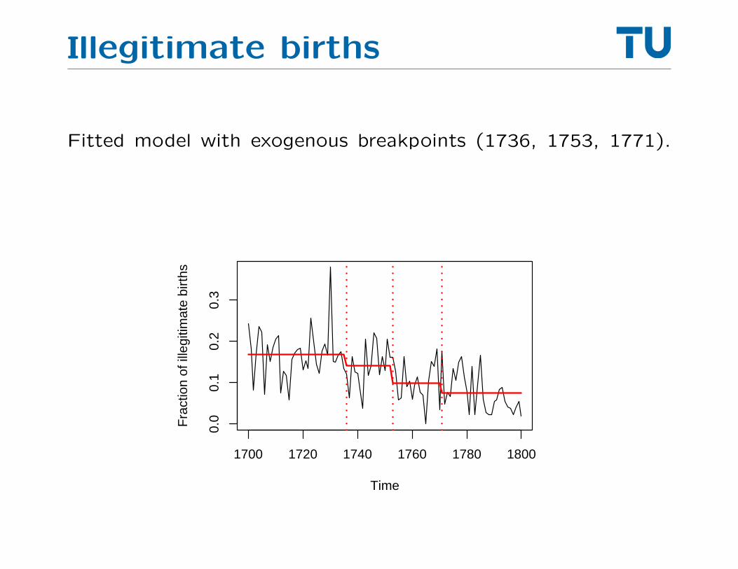
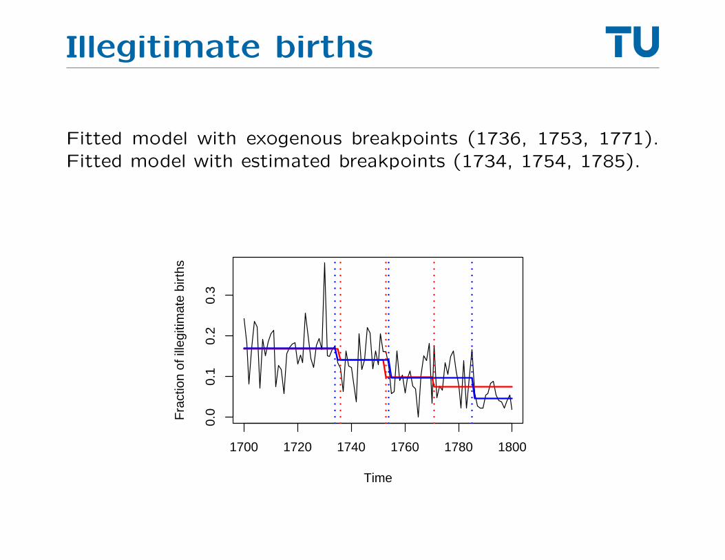
Illegitimate births
Fitted model with exogenous breakpoints (1736, 1753, 1771).Fitted model with estimated breakpoints (1734, 1754, 1785).
Time
Fra
ctio
n of
ille
gitim
ate
birt
hs
1700 1720 1740 1760 1780 1800
0.0
0.1
0.2
0.3
Illegitimate births
Fitted model with exogenous breakpoints (1736, 1753, 1771).Fitted model with estimated breakpoints (1734, 1754, 1785).
Time
Fra
ctio
n of
ille
gitim
ate
birt
hs
1700 1720 1740 1760 1780 1800
0.0
0.1
0.2
0.3
Illegitimate births
Fitted model with exogenous breakpoints (1736, 1753, 1771).Fitted model with estimated breakpoints (1734, 1754, 1785).
Time
Fra
ctio
n of
ille
gitim
ate
birt
hs
1700 1720 1740 1760 1780 1800
0.0
0.1
0.2
0.3

Software
All methods implemented in the R system for statistical com-
puting and graphics
http://www.R-project.org/
in the contributed package strucchange.
Both are available under the GPL (General Public Licence) from
the Comprehensive R Archive Network (CRAN):
http://CRAN.R-project.org/
Software
R> M1.model <- dm ~ dy2 + dR + dR1 + dp + ecm.res + seasonR> scus <- efp(M1.model, type = "Score-CUSUM", data = GermanM1)R> plot(scus, functional = "meanL2")
Software
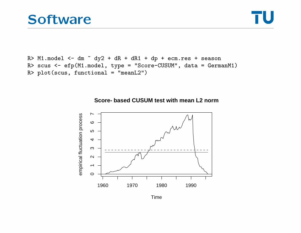
R> M1.model <- dm ~ dy2 + dR + dR1 + dp + ecm.res + seasonR> scus <- efp(M1.model, type = "Score-CUSUM", data = GermanM1)R> plot(scus, functional = "meanL2")
Score−based CUSUM test with mean L2 norm
Time
empi
rical
fluc
tuat
ion
proc
ess
1960 1970 1980 1990
01
23
45
67
Software
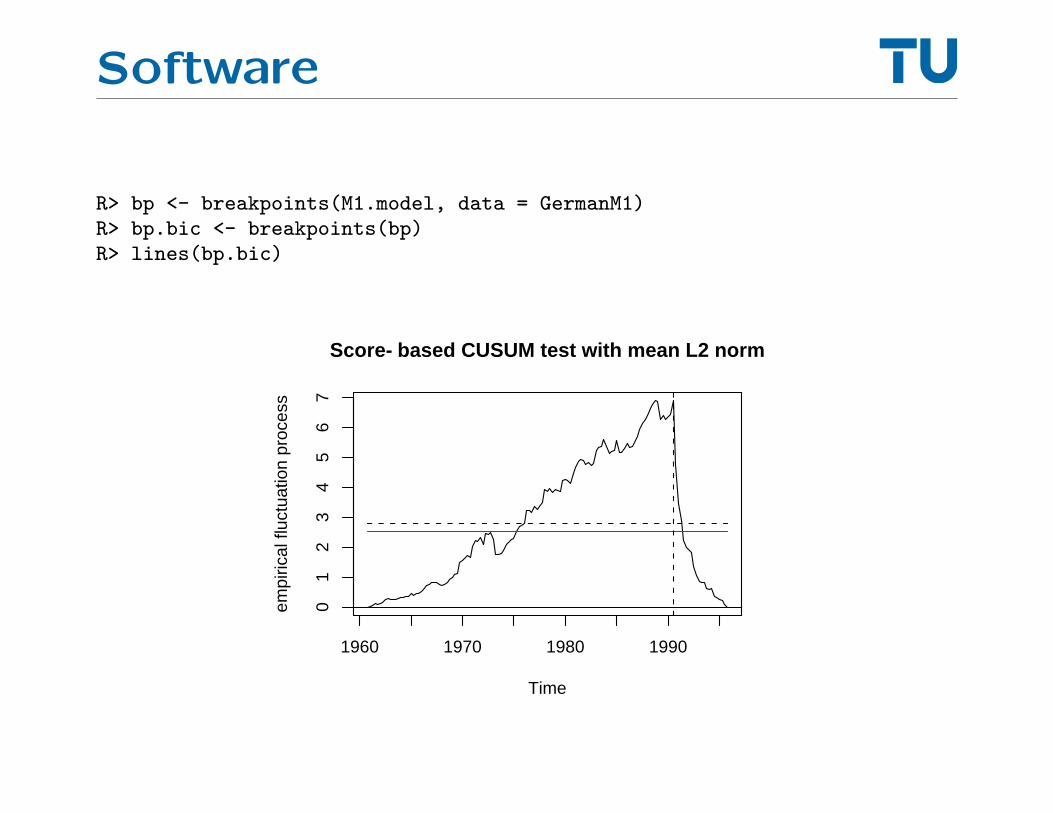
R> bp <- breakpoints(M1.model, data = GermanM1)R> bp.bic <- breakpoints(bp)R> lines(bp.bic)
Score−based CUSUM test with mean L2 norm
Time
empi
rical
fluc
tuat
ion
proc
ess
1960 1970 1980 1990
01
23
45
67
Software
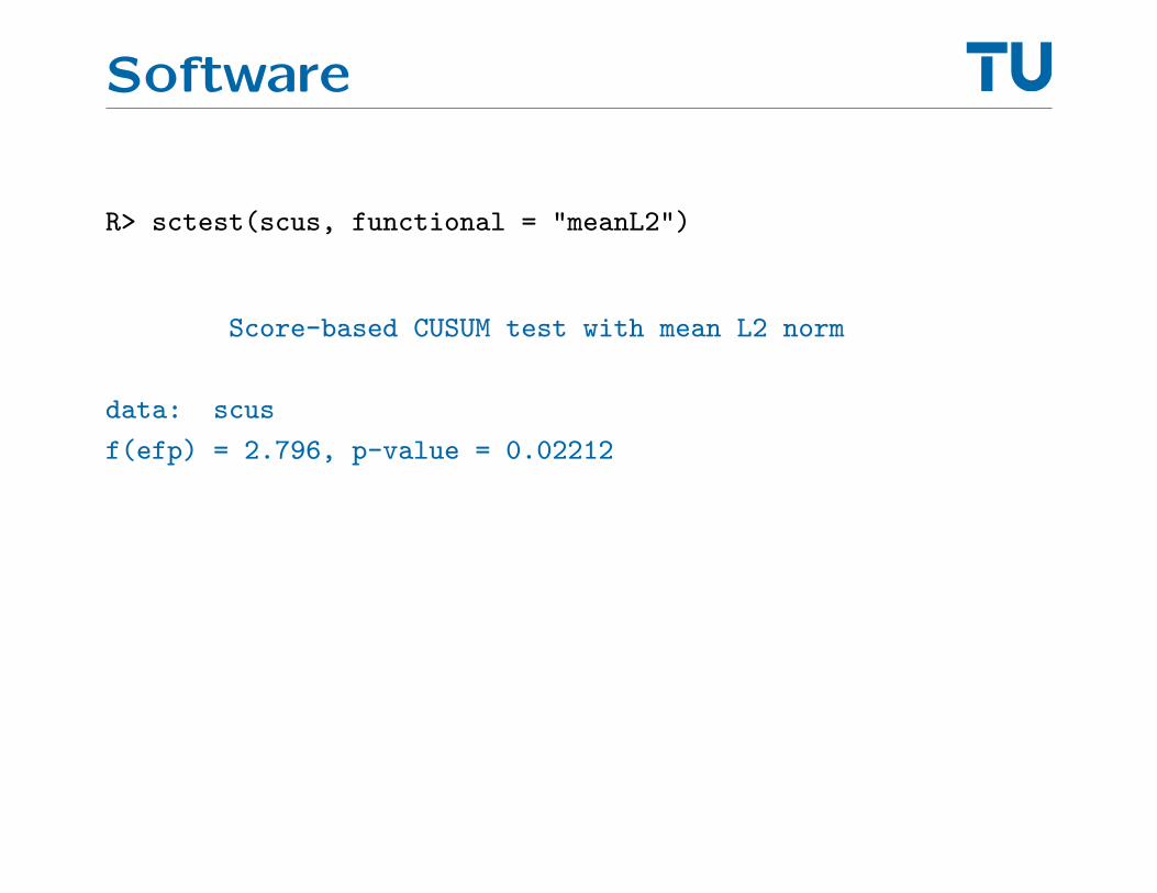
R> sctest(scus, functional = "meanL2")
Score-based CUSUM test with mean L2 norm
data: scus
f(efp) = 2.796, p-value = 0.02212