Anthony Greene 1

Simple Hypothesis Testing Detecting Statistical Differences

In The Simplest Case:

and are both known

I The Logic of Hypothesis Testing:

The Null Hypothesis

II The Tail Region, Critical Values: α

III Type I and Type II Error

Anthony Greene 2

The Fundamental Idea 1. Apply a treatment to a sample

2. Measure the sample mean (this means using a

sampling distribution) after the treatment and

compare it to the original mean

3. Remembering differences always exist due to

chance, figure out the odds that your

experimental difference is due to chance.

4. If its too unlikely that chance was the reason for

the difference, conclude that you have an effect

Anthony Greene 3

Null and Alternative

Hypotheses

Null hypothesis: A hypothesis to be tested. We use the

symbol H0 to represent the null hypothesis.

Alternative hypothesis: A hypothesis to be considered as

an alternate to the null hypothesis. We use the symbol Ha to

represent the alternative hypothesis.

Anthony Greene 4

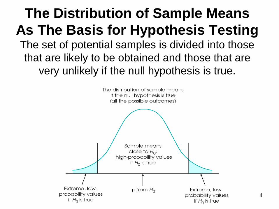
The Distribution of Sample Means

As The Basis for Hypothesis Testing The set of potential samples is divided into those

that are likely to be obtained and those that are

very unlikely if the null hypothesis is true.

Anthony Greene 5

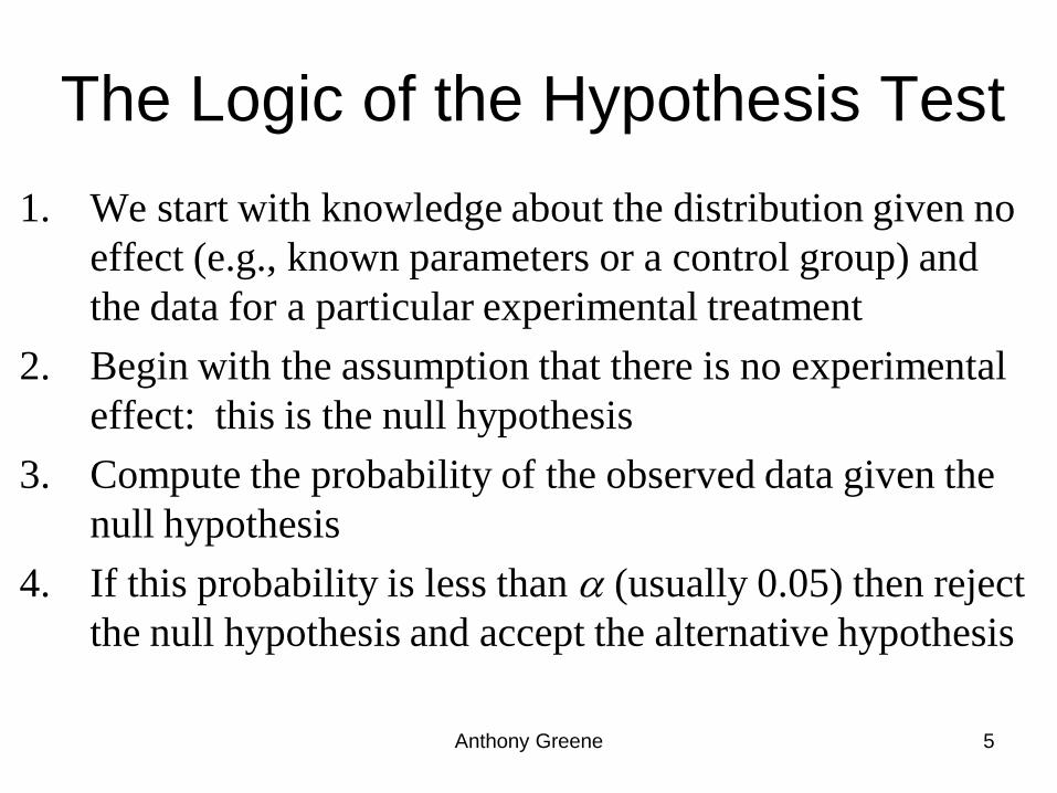
The Logic of the Hypothesis Test

1. We start with knowledge about the distribution given no

effect (e.g., known parameters or a control group) and

the data for a particular experimental treatment

2. Begin with the assumption that there is no experimental

effect: this is the null hypothesis

3. Compute the probability of the observed data given the

null hypothesis

4. If this probability is less than (usually 0.05) then reject

the null hypothesis and accept the alternative hypothesis

Anthony Greene 6

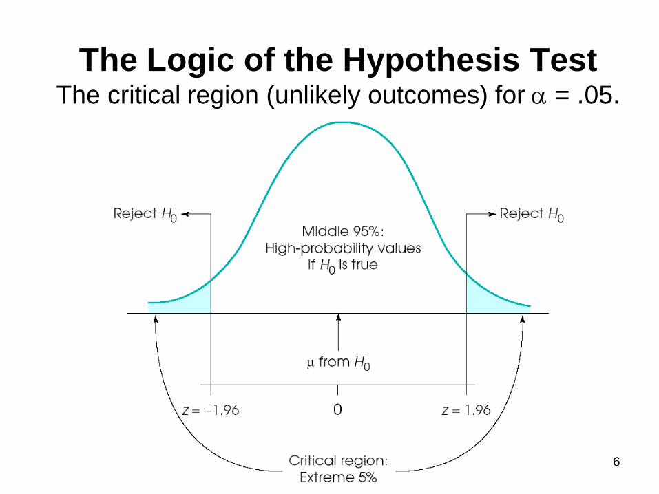
The Logic of the Hypothesis Test The critical region (unlikely outcomes) for = .05.

Anthony Greene 7

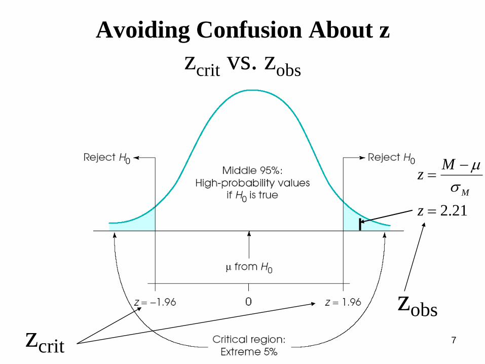
Avoiding Confusion About z

zcrit vs. zobs

zcrit

zobs

21.2

z

Mz

M

Anthony Greene 8

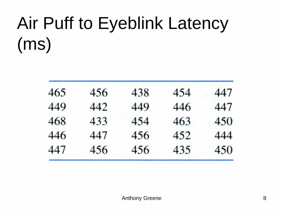
Air Puff to Eyeblink Latency

(ms)

Anthony Greene 9

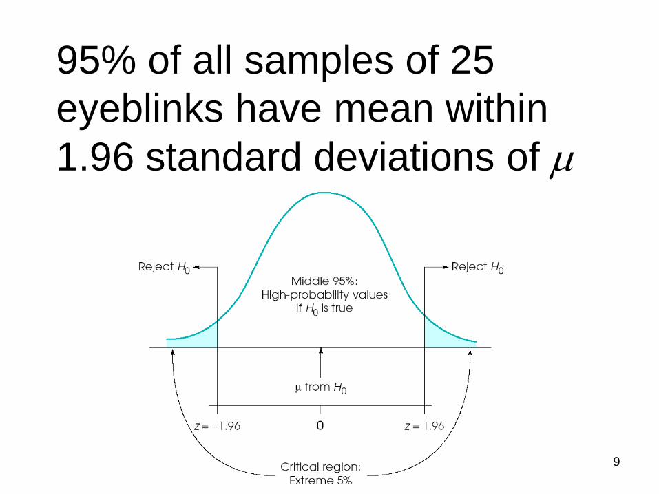
95% of all samples of 25

eyeblinks have mean within

1.96 standard deviations of

Anthony Greene 10

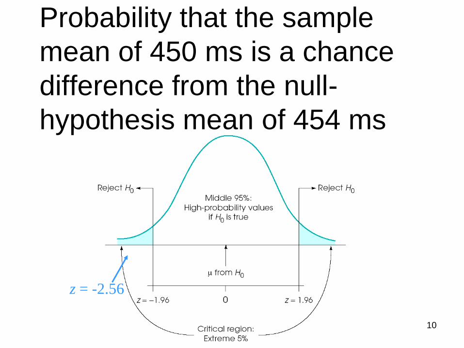
Probability that the sample

mean of 450 ms is a chance

difference from the null-

hypothesis mean of 454 ms

z = -2.56

Anthony Greene 11

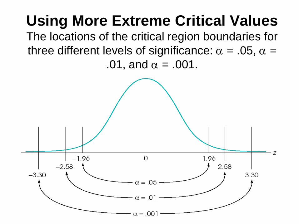
Using More Extreme Critical Values The locations of the critical region boundaries for

three different levels of significance: = .05, =

.01, and = .001.

Anthony Greene 12

Test Statistic, Rejection

Region, Nonrejection Region,

Critical Values

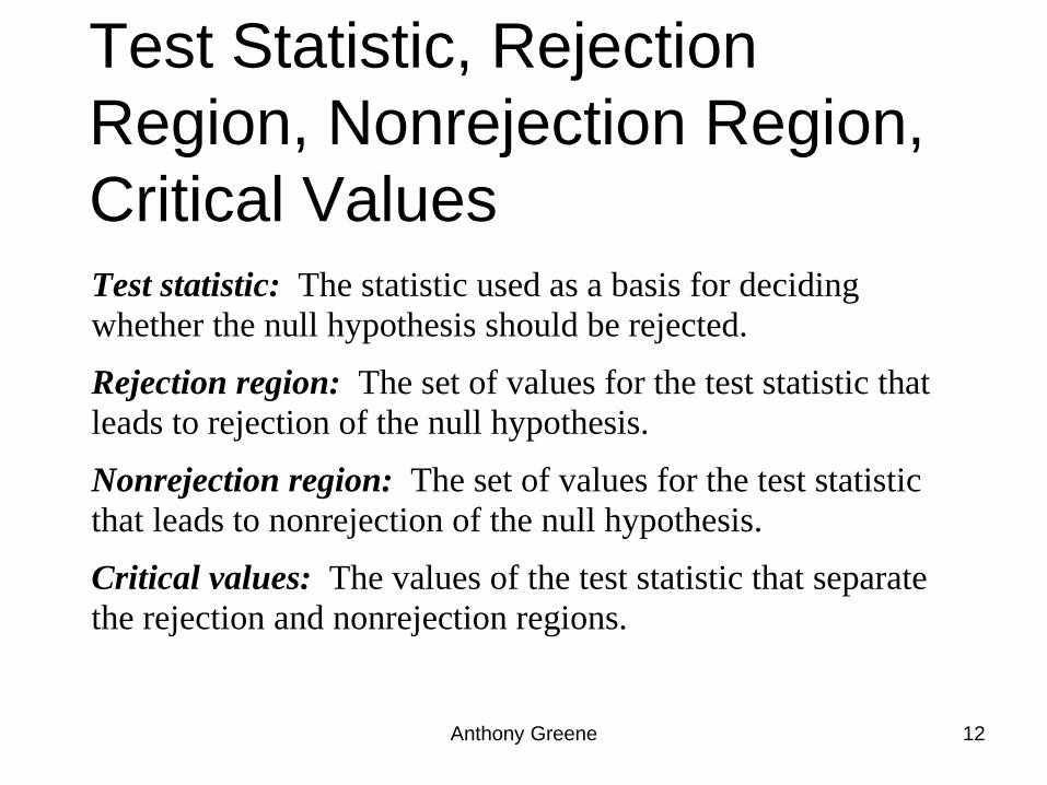
Test statistic: The statistic used as a basis for deciding

whether the null hypothesis should be rejected.

Rejection region: The set of values for the test statistic that

leads to rejection of the null hypothesis.

Nonrejection region: The set of values for the test statistic

that leads to nonrejection of the null hypothesis.

Critical values: The values of the test statistic that separate

the rejection and nonrejection regions.

Anthony Greene 13

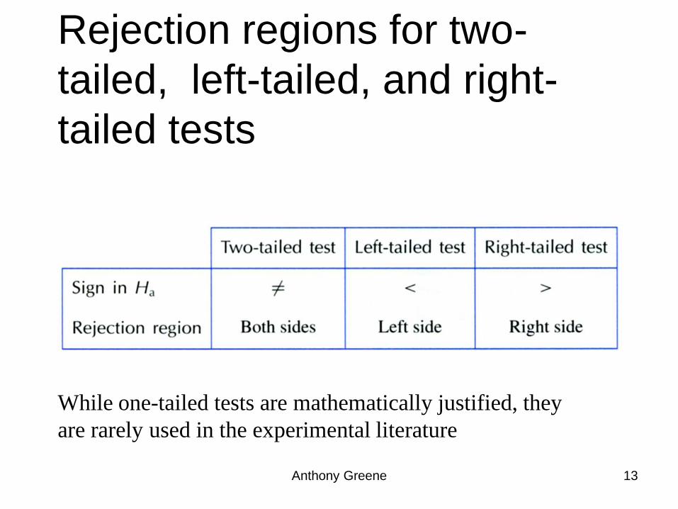
Rejection regions for two-

tailed, left-tailed, and right-

tailed tests

While one-tailed tests are mathematically justified, they

are rarely used in the experimental literature

Anthony Greene 14

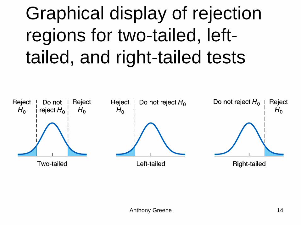
Graphical display of rejection

regions for two-tailed, left-

tailed, and right-tailed tests

Anthony Greene 15

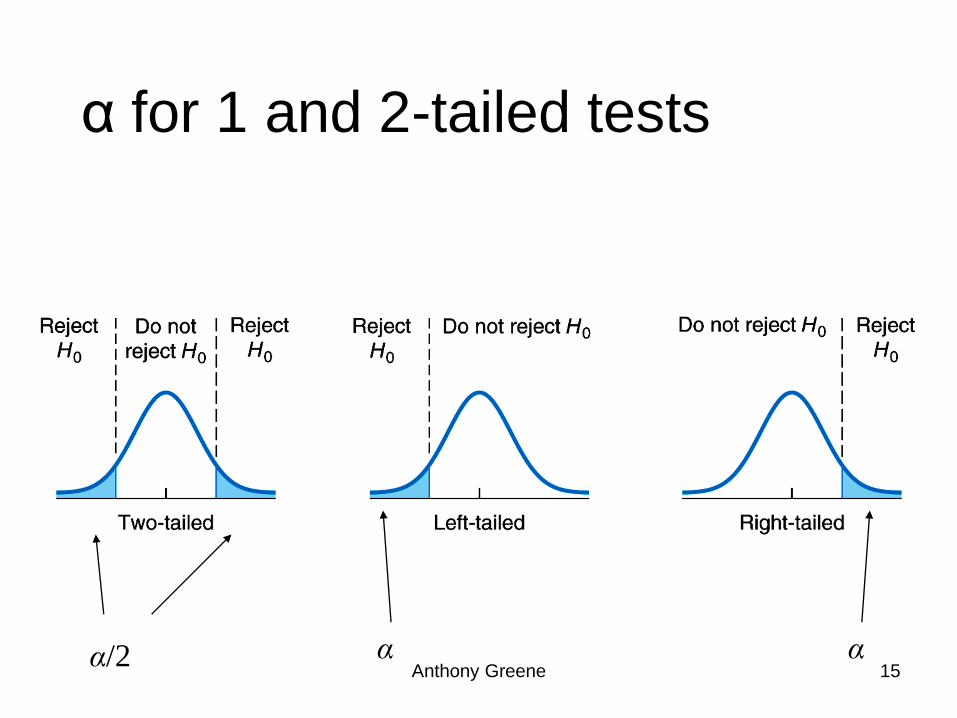
α for 1 and 2-tailed tests

α/2 α α

Anthony Greene 16

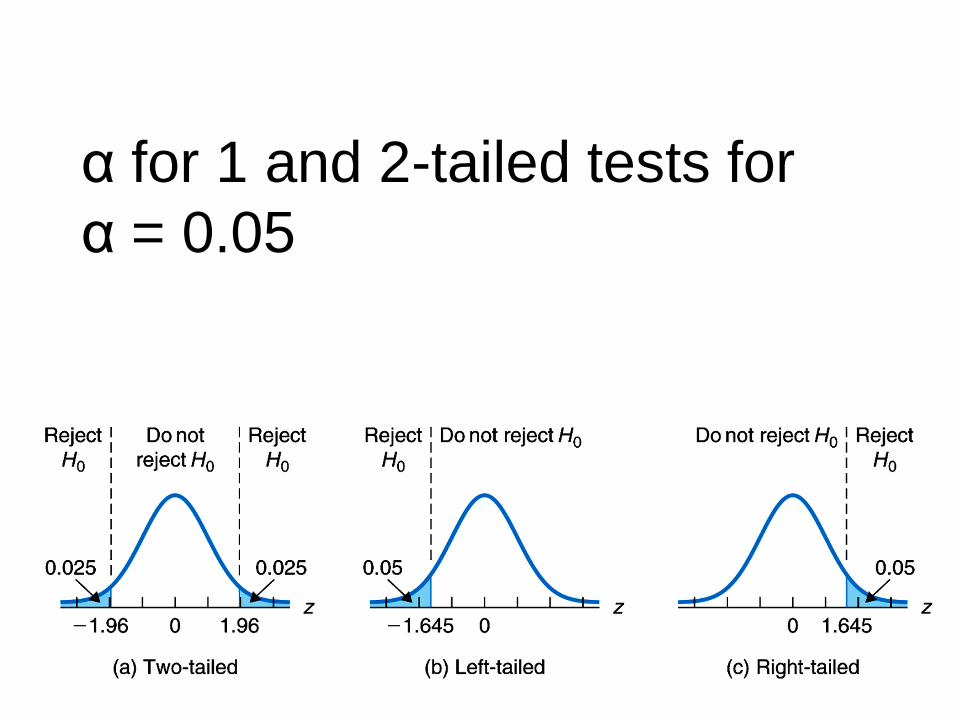
α for 1 and 2-tailed tests for

α = 0.05

Anthony Greene 17

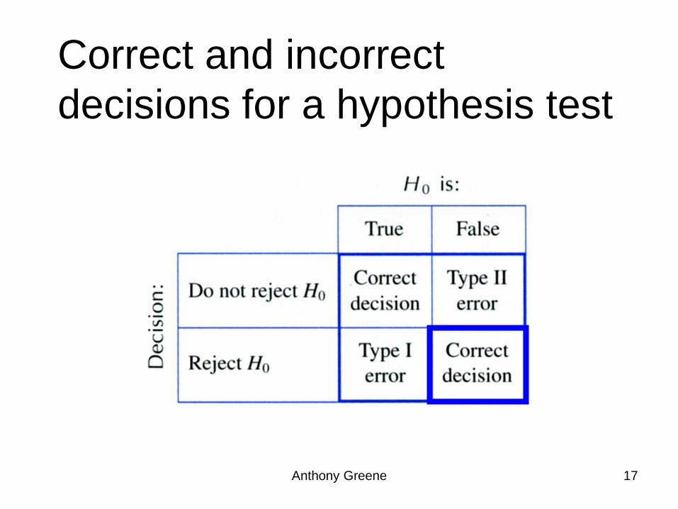
Correct and incorrect

decisions for a hypothesis test

Anthony Greene 18

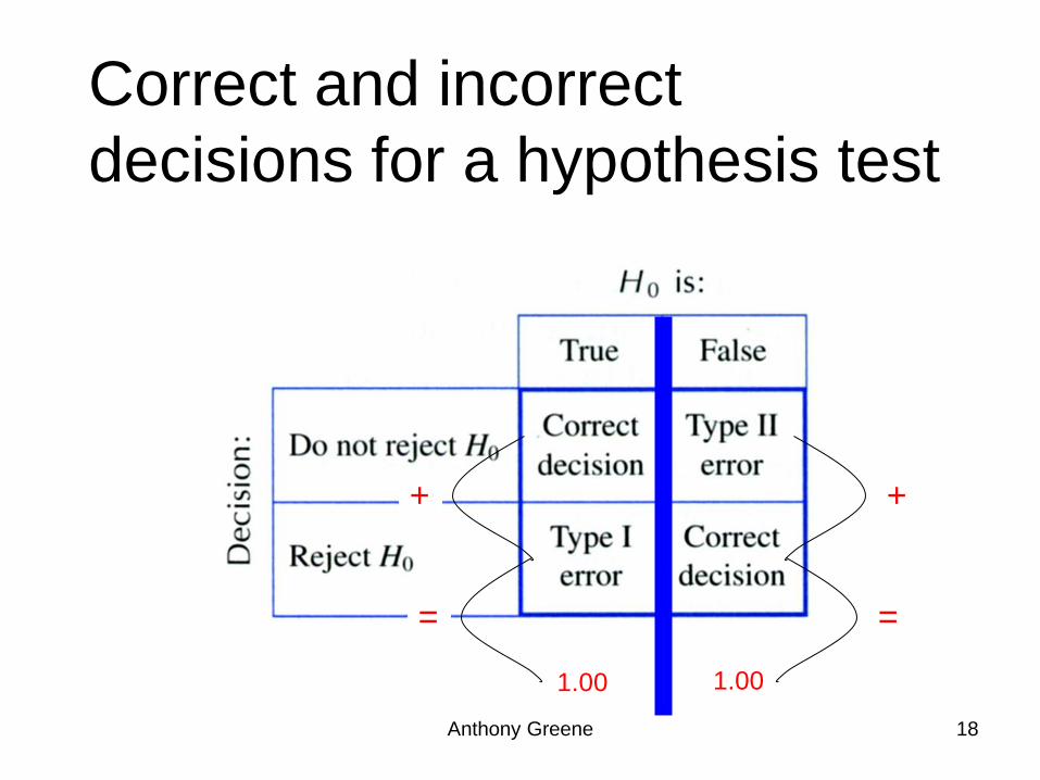
Correct and incorrect

decisions for a hypothesis test

+

=

+

=

1.00 1.00

Anthony Greene 19

Type I and Type II Errors

Type I error: Rejecting the null hypothesis when it is in

fact true.

Type II error: Not rejecting the null hypothesis when it is

in fact false.

Anthony Greene 20

Significance Level

The probability of making a Type I error, that is, of rejecting

a true null hypothesis, is called the significance level, , of a

hypothesis test.

That is, given the null hypothesis, if the liklihood of the

observed data is small, (less than ) we reject the null

hypothesis. However, by rejecting it, there is still an

(e.g., 0.05) probability that rejecting the null hypothesis

was the incorrect decision.

Anthony Greene 21

Relation Between Type I and

Type II Error Probabilities

For a fixed sample size, the smaller we specify the

significance level, , (i.e., lower probability of type I error)

the larger will be the probability, b, of not rejecting a false

null hypothesis.

Another way to say this is that the lower we set the

significance, the harder it is to detect a true experimental

effect.

Anthony Greene 22

Possible Conclusions for a

Hypothesis Test

• If the null hypothesis is rejected, we conclude

that the alternative hypothesis is true.

• If the null hypothesis is not rejected, we conclude

that the data do not provide sufficient evidence to

support the alternative hypothesis.

Anthony Greene 23

Critical Values, α = P(type I error)

Suppose a hypothesis test is to be performed at a specified

significance level, . Then the critical value(s) must be

chosen so that if the null hypothesis is true, the probability

is equal to that the test statistic will fall in the rejection

region.

Anthony Greene 24

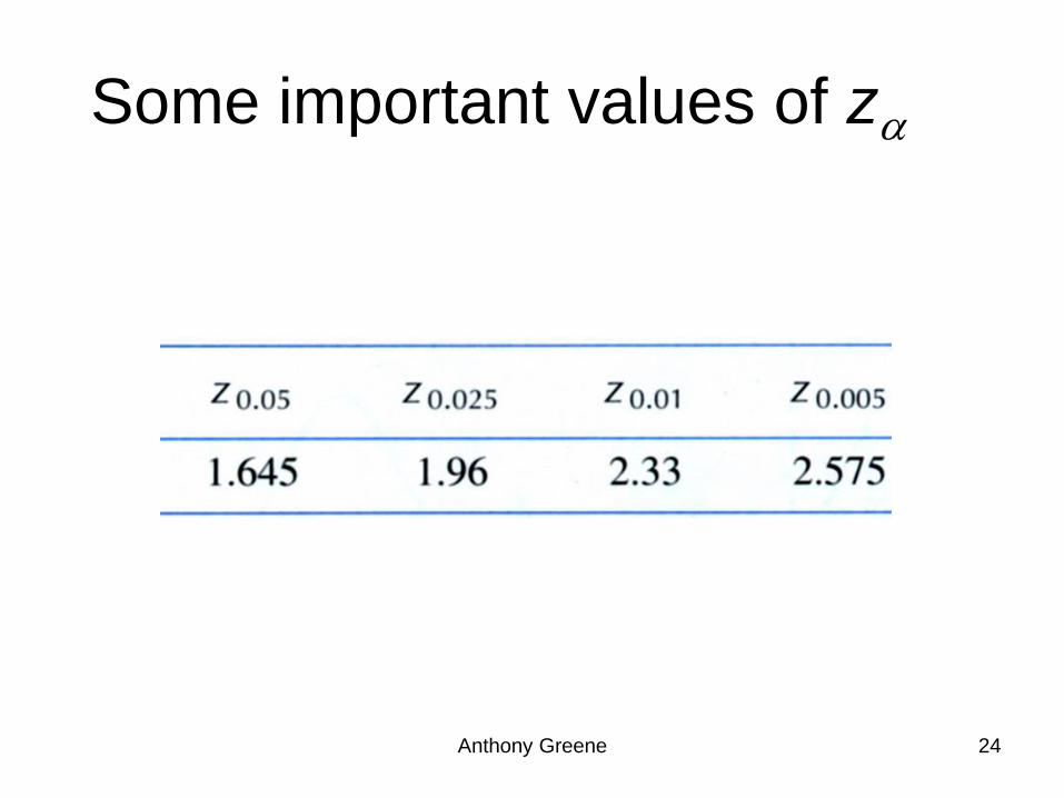
Some important values of z

25

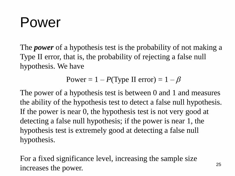
Power

The power of a hypothesis test is the probability of not making a

Type II error, that is, the probability of rejecting a false null

hypothesis. We have

Power = 1 – P(Type II error) = 1 – b

The power of a hypothesis test is between 0 and 1 and measures

the ability of the hypothesis test to detect a false null hypothesis.

If the power is near 0, the hypothesis test is not very good at

detecting a false null hypothesis; if the power is near 1, the

hypothesis test is extremely good at detecting a false null

hypothesis.

For a fixed significance level, increasing the sample size

increases the power.

Anthony Greene 26

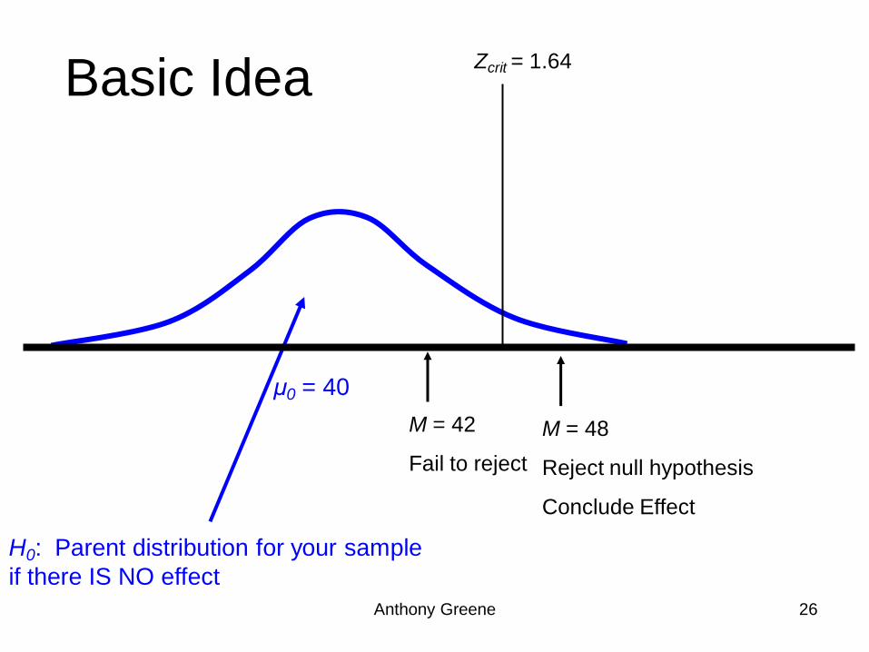
Basic Idea

H0: Parent distribution for your sample

if there IS NO effect

μ0 = 40

Zcrit = 1.64

M = 42

Fail to reject

M = 48

Reject null hypothesis

Conclude Effect

Anthony Greene 27

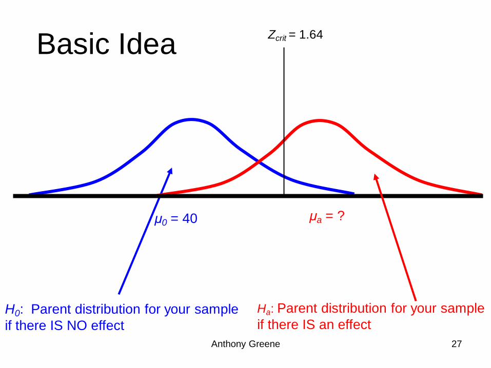
Basic Idea

H0: Parent distribution for your sample

if there IS NO effect

Ha: Parent distribution for your sample

if there IS an effect

μ0 = 40 μa = ?

Zcrit = 1.64

Anthony Greene 28

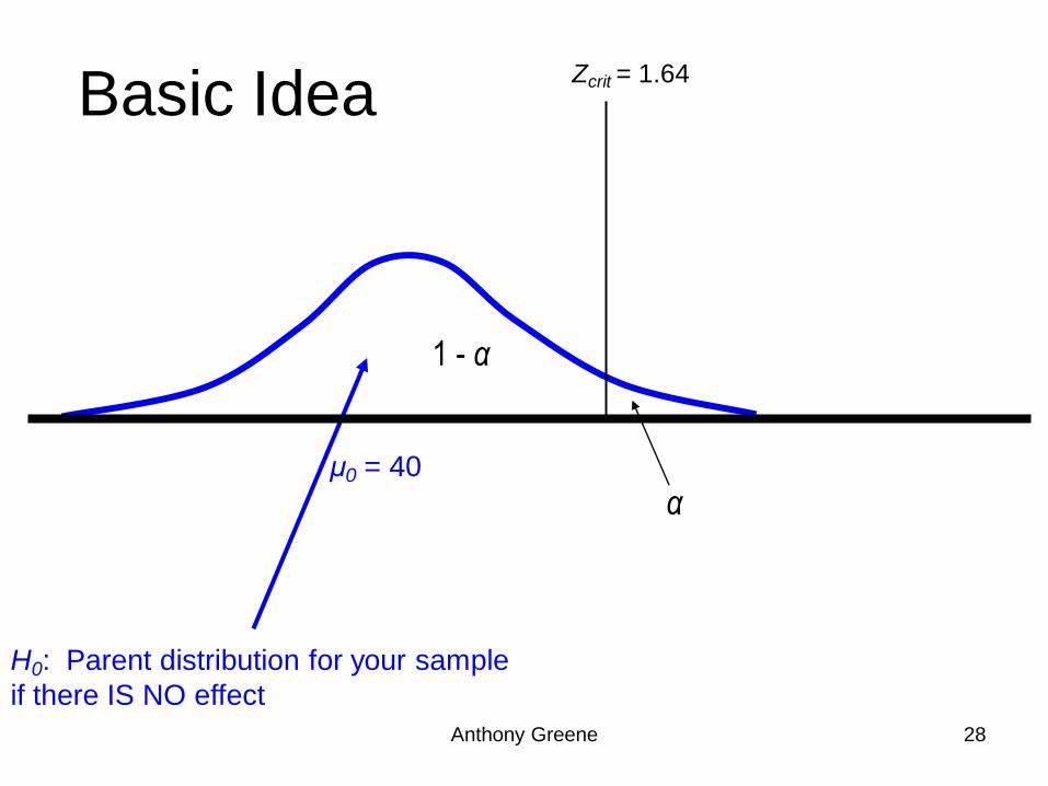
Basic Idea

H0: Parent distribution for your sample

if there IS NO effect

μ0 = 40

Zcrit = 1.64

α

1 - α

Anthony Greene 29

Basic Idea

Ha: Parent distribution for your sample

if there IS an effect

μa = ?

Zcrit = 1.64

β 1 - β

Anthony Greene 30

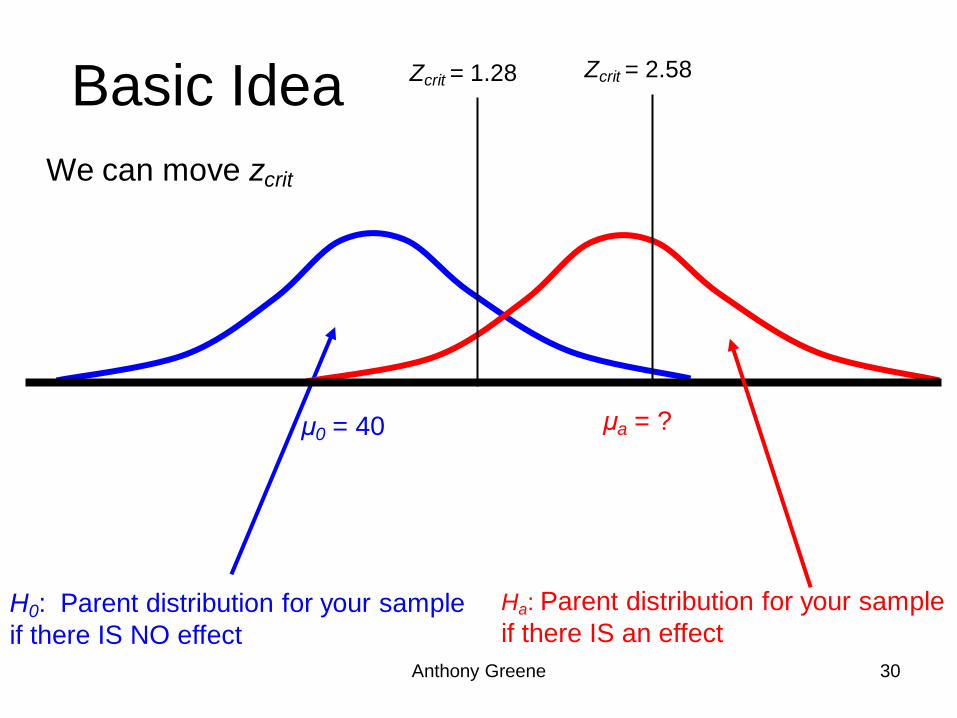
Basic Idea

H0: Parent distribution for your sample

if there IS NO effect

Ha: Parent distribution for your sample

if there IS an effect

μ0 = 40 μa = ?

Zcrit = 1.28

We can move zcrit

Zcrit = 2.58

Anthony Greene 31

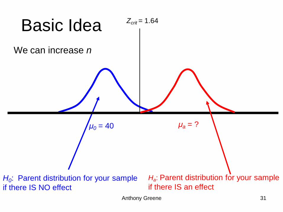
Basic Idea

H0: Parent distribution for your sample

if there IS NO effect

Ha: Parent distribution for your sample

if there IS an effect

μ0 = 40 μa = ?

Zcrit = 1.64

We can increase n

Anthony Greene 32

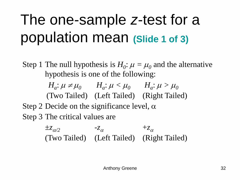
The one-sample z-test for a

population mean (Slide 1 of 3)

Step 1 The null hypothesis is H0: = 0 and the alternative

hypothesis is one of the following:

Ha: 0 Ha: < 0 Ha: > 0

(Two Tailed) (Left Tailed) (Right Tailed)

Step 2 Decide on the significance level,

Step 3 The critical values are

±z/2 -z +z

(Two Tailed) (Left Tailed) (Right Tailed)

Anthony Greene 33

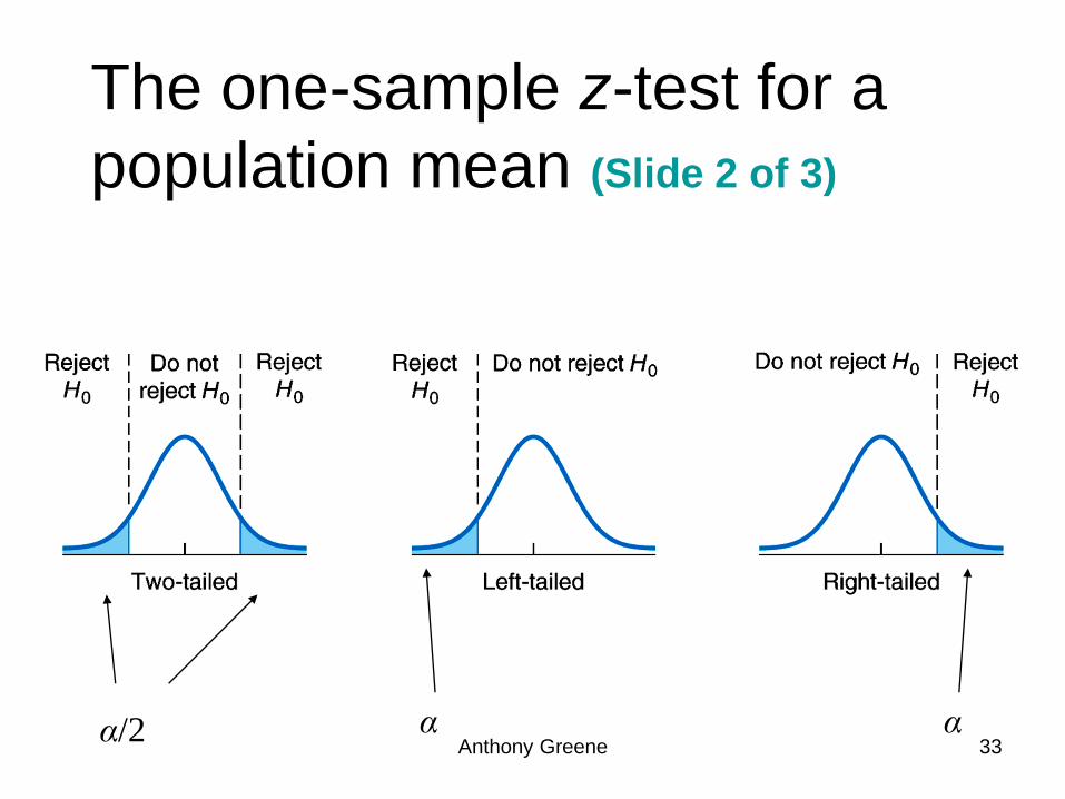
The one-sample z-test for a

population mean (Slide 2 of 3)

α/2 α α

Anthony Greene 34

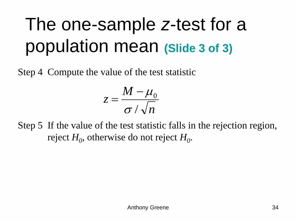
The one-sample z-test for a

population mean (Slide 3 of 3)

Step 4 Compute the value of the test statistic

Step 5 If the value of the test statistic falls in the rejection region,

reject H0, otherwise do not reject H0.

n

Mz

/

0

Anthony Greene 35

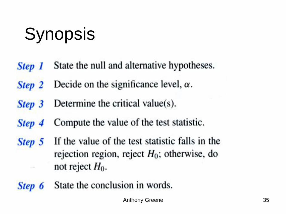
Synopsis

Anthony Greene 36

P-Value

To obtain the P-value of a hypothesis test, we compute,

assuming the null hypothesis is true, the probability of

observing a value of the test statistic as extreme or more

extreme than that observed. By “extreme” we mean “far

from what we would expect to observe if the null

hypothesis were true.” We use the letter P to denote the

P-value. The P-value is also referred to as the observed

significance level or the probability value.

Anthony Greene 37

P-value for a z-test

•Two-tailed test: The P-value is the probability of observing a value of the test statistic z at least as large in magnitude as the value actually observed, which is the area under the standard normal curve that lies outside the interval from –|z0| to |z0|,

•Left-tailed test: The P-value is the probability of observing a value of the test statistic z as small as or smaller than the value actually observed, which is the area under the standard normal curve that lies to the left of z0,

•Right-tailed test: The P-value is the probability of observing a value of the test statistic z as large as or larger than the value actually observed, which is the area under the standard normal curve that lies to the right of z0,

Anthony Greene 38

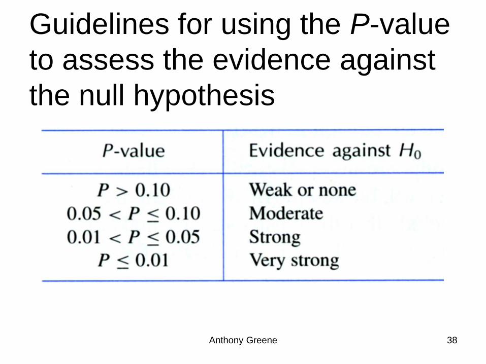
Guidelines for using the P-value

to assess the evidence against

the null hypothesis