FYS-KJM 4740 Chap1-2...FYS-KJM 4740 Chap 1 Bloch equations and main principles FYS-KJEM 4740...

3/4/2011

1

MRI

FYS-KJM 4740

Chap 1

Bloch equations and main

principles

FYS-KJEM 4740 Frédéric Courivaud (PhD) 2

z

y

x

B0

M

ωL

Mz

ωL

Figure Error! No text of specified style in document.-1. The magnetic moment M rotates around

The magnetic moment M rotates around the static B-field at the Larmor frequency

)( BMM

×= γdt

d

FYS-KJM 4740 3

The Bloch equation

ω0 (rad/s) = γ (rad/s/Tesla) x B0 (Tesla)

γhydrogen = 2.68 *108 rad/s/Tesla

fL (MHz) = γ (MHz/Tesla) x B0 (Tesla)

γhydrogen = 42.58 MHz/Tesla

/2π

Joseph Larmor

z

y

x

B0

M

ωL

Mz

ωL

Larmor equation

FYS-KJM 4740 AtleBjørnerud 4

y

x

zω0

Laboratory frame

B0

y`

x`

z`

B0

Rotating frame

Rotating frame of reference

FYS-KJEM 4740 5

In MRI, short RF pulses are used toTo change the direction of the magnetization

M

To get M to rotate around x or y axis,A linearly polarized magnetic field B1 is used during short time (pulse) to get M to rotate

around B1 axis

y`

x`

z

B1

M

Flipping away the Magnetization from its equilibrium

FYS-KJEM 4740 6

3/4/2011

2

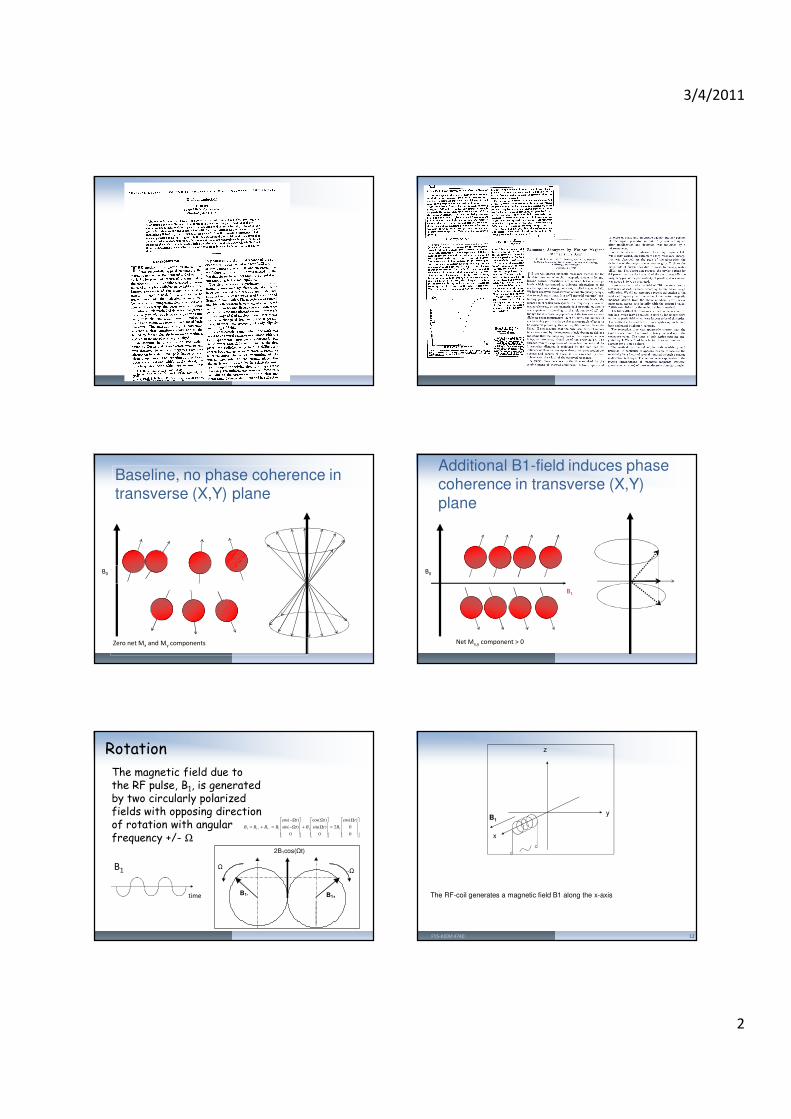
Baseline, no phase coherence in transverse (X,Y) plane

B0

Zero net Mx and My components

Additional B1-field induces phase coherence in transverse (X,Y)

plane

B0

Net Mx,y component > 0

B1

The magnetic field due to the RF pulse, B1, is generatedby two circularly polarizedfields with opposing directionof rotation with angularfrequency +/- Ω

B1

time

Rotation

B1+ B1-

-Ω Ω

2B1cos(Ωt)

Ω

=

Ω

Ω

+

Ω−

Ω−

=+= −+

0

0

)cos(

2

0

)sin(

)cos(

0

)sin(

)cos(

111111

t

Bt

t

Bt

t

BBBB

z

y

x

B1

The RF-coil generates a magnetic field B1 along the x-axis

FYS-KJEM 4740 12

3/4/2011

3

z

y

x y’

z’

x’

Ω

Ω

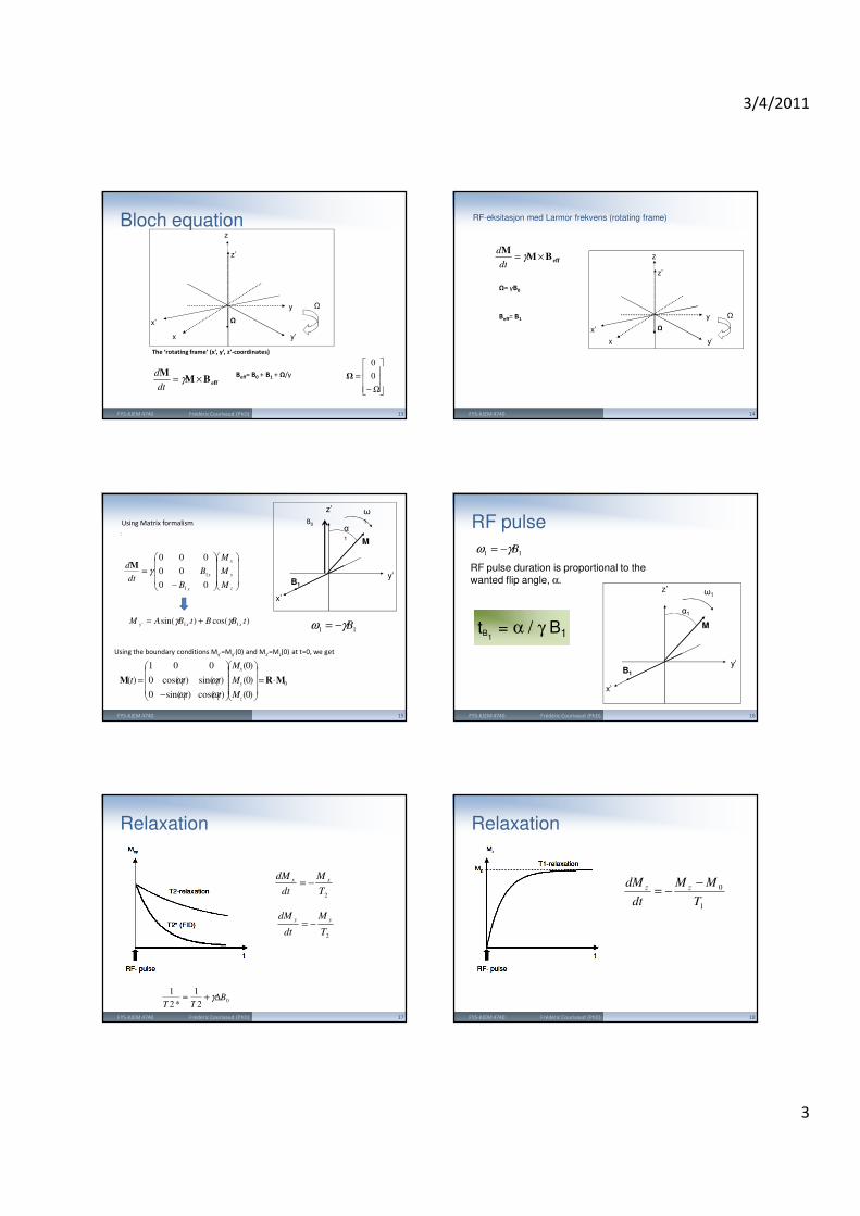
The ‘rotating frame’ (x’, y’, z’-coordinates)

effBMM

×= γdt

d Beff= B0 + B1 + Ω/γ

Ω−

= 0

0

Ω

Bloch equation


RF-eksitasjon med Larmor frekvens (rotating frame)

effBMM

×= γdt

d

Beff= B1

Ω= γB0

z

y

x y’

z’

x’

Ω

Ω

FYS-KJEM 4740 14

Using Matrix formalism

z’

y’

x’

B1

α1 M

ω1B0

−

=

z

y

x

x

x

M

M

M

B

Bdt

d

00

00

000

1

1γM

0

11

11

)0(

)0(

)0(

)cos()sin(0

)sin()cos(0

001

)( MRM ⋅=

−

=

z

y

x

M

M

M

tt

ttt

ωω

ωω

)cos()sin( '1'1' tBBtBAM xxy γγ +=

:

Using the boundary conditions My’=My’(0) and Mz’=Mz(0) at t=0, we get

11 Bγω −=

FYS-KJEM 4740 15

RF pulse duration is proportional to the

wanted flip angle, α.

tB1

= α / γ B1

z’

y’

x’

B1

α1

M

ω1

11 Bγω −=

RF pulse


2T

M

dt

dM xx −=

2T

M

dt

dM yy−=

02

1

*2

1B

TT∆+= γ

Relaxation


1

0

T

MM

dt

dM zz −−=

Relaxation


3/4/2011

4

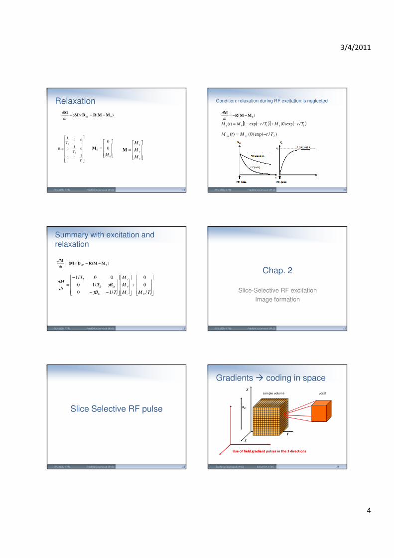
)( 0MMRBMM

−−×= effdt

dγ

=

1

2

2

100

01

0

001

T

T

T

R

=

0

0 0

0

M

M

=

z

y

x

M

M

M

M

Relaxation


( )[ ] ( )110 /exp)0(/exp1)( TtMTtMtM zz −+−−=

)/exp()0()( 2TtMtM xyxy −=

Condition: relaxation during RF excitation is neglected


)( 0MMRM

−−=dt

d

)( 0MMRBMM

−−×= effdt

dγ

+

−−

−

−

=

10'

'

'

11

12

2

/

0

0

/10

/10

00/1

TMM

M

M

TB

BT

T

dt

dM

z

y

x

x

x

γ

γ

Summary with excitation and relaxation


Chap. 2

Slice-Selective RF excitation

Image formation


Slice Selective RF pulse


Z

X

Y

sample volume voxel

B0

Use of field gradient pulses in the 3 directions

Gradients coding in space

Frédéric Courivaud (PhD) KJEM/FYS 4740 24

3/4/2011

5

z

x

y

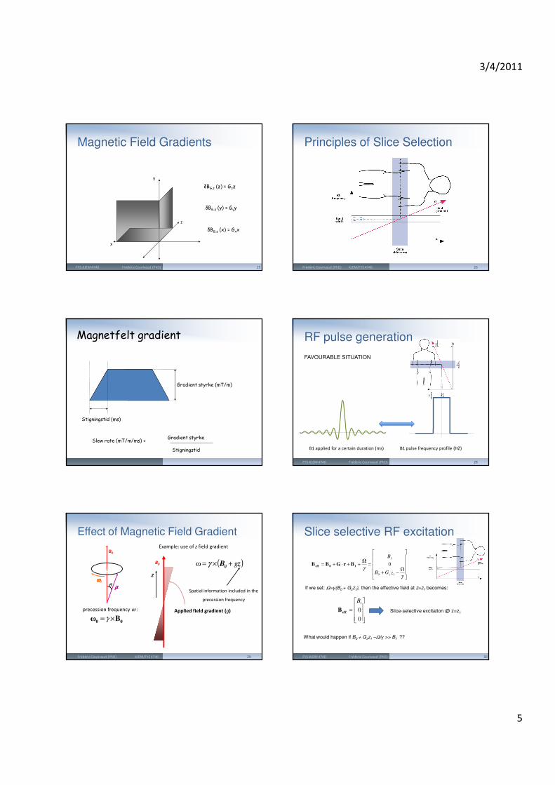
δBG,z (z) = Gzz

δBG,z (y) = Gyy

δBG,z (x) = Gxx

Magnetic Field Gradients


Principles of Slice Selection


Magnetfelt gradient

Stigningstid (ms)

Gradient styrke (mT/m)

Slew rate (mT/m/ms) = Gradient styrke

Stigningstid

FAVOURABLE SITUATION

28FYS-KJEM 4740 Frédéric Courivaud (PhD)

B1 applied for a certain duration (ms) B1 pulse frequency profile (HZ)

RF pulse generation

θ

B0

µµµµωωωω0

00 Bω ×=γprecession frequency ω :

( )zB0

g+×=γω

Spatial information included in the

precession frequency

Effect of Magnetic Field GradientExample: use of z field gradient

Applied field gradient (g)

B0

Z


Ω−+

=++⋅+=

γ

γ10

1

0

zGB

B

z

ΩBrGBB 10eff

If we set: Ω=γ(B0 + Gzz1), then the effective field at z=z1 becomes:

=

0

0

1B

effB

What would happen if B0 + Gzz1 –Ω/γ >> B1 ??

Slice-selective excitation @ z=z1

Slice selective RF excitation


3/4/2011

6

+

−−

−⋅−

⋅−

=

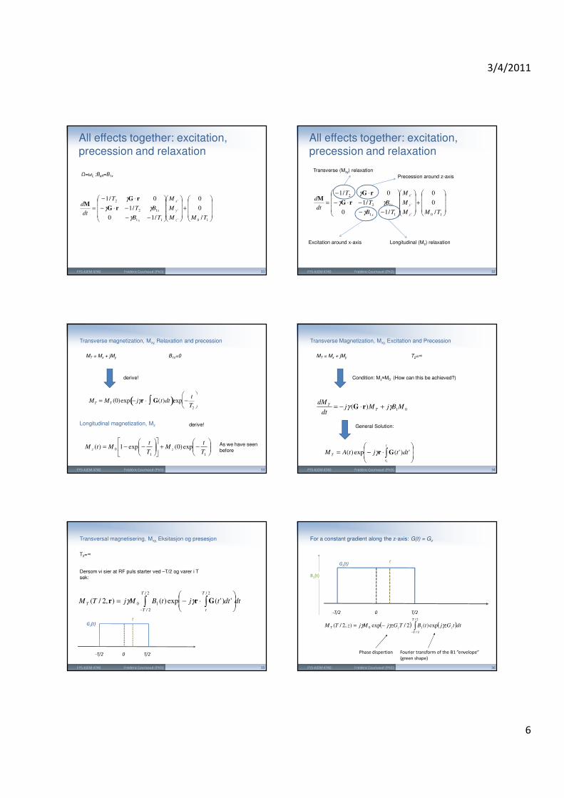
10'

'

'

11

12

2

/

0

0

/10

/1

0/1

TMM

M

M

TB

BT

T

dt

d

z

y

x

x

x

γ

γγ

γ

rG

rGM

Ω=ωL ;Beff=B1x

All effects together: excitation, precession and relaxation


+

−−

−⋅−

⋅−

=

10'

'

'

11

12

2

/

0

0

/10

/1

0/1

TMM

M

M

TB

BT

T

dt

d

z

y

x

x

x

γ

γγ

γ

rG

rGM

Precession around z-axis

Excitation around x-axis

Transverse (Mxy) relaxation

Longitudinal (Mz) relaxation

All effects together: excitation, precession and relaxation


Transverse magnetization, Mxy, Relaxation and precession

MT = Mx + jMy

MT = MT (0)exp − jγr ⋅ G∫ (t)dt( )exp −t

T2

B1x=0

derive!

Longitudinal magnetization, Mz

−+

−−=

11

0 exp)0(exp1)(T

tM

T

tMtM zz

derive!

As we have seen

before


Transverse Magnetization, Mxy, Excitation and Precession

MT = Mx + jMy T2=∞

01)( MBjMjdt

dMT

T γγ +⋅−= rG

Condition: Mz≈M0 (How can this be achieved?)

⋅−= ∫

t

t

T dttjtAM

1

')'(exp)( Grγ

General Solution:


Transversal magnetisering, Mxy, Eksitasjon og presesjon

Dersom vi sier at RF puls starter ved –T/2 og varer i T

sek:

T2=∞

dtdttjtBMjTM

T

T

T

t

T ∫ ∫−

⋅−=

2/

2/

2/

10 ')'(exp)(),2/( Grr γγ

Gz(t)

-T/2 0 T/2

t


( ) ( )∫−

−=2/

2/

10 exp)(2/exp),2/(

T

T

zzT dttzGjtBTzGjMjzTM γγγ

Phase dispertion Fourier transform of the B1 ”envelope”

(green shape)

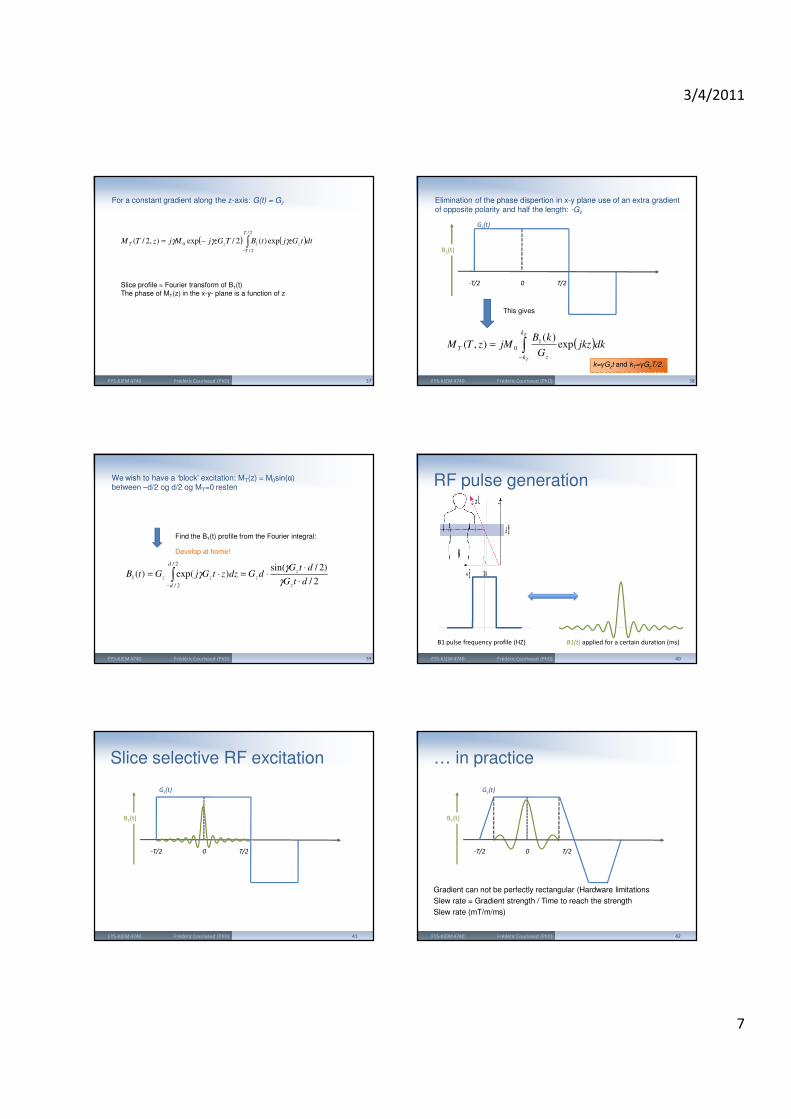
For a constant gradient along the z-axis: G(t) = Gz

B1(t)

Gz(t)

-T/2 0 T/2

t


3/4/2011

7

( ) ( )∫−

−=2/

2/

10 exp)(2/exp),2/(

T

T

zzT dttzGjtBTzGjMjzTM γγγ

Slice profile = Fourier transform of B1(t)

The phase of MT(z) in the x-y- plane is a function of z

For a constant gradient along the z-axis: G(t) = Gz


Elimination of the phase dispertion in x-y plane use of an extra gradient of opposite polarity and half the length: -Gz

( )∫−

=T

T

k

k z

T dkjkzG

kBjMzTM exp

)(),( 1

0

This gives

k=γGzt and kT=γGzT/2.

B1(t)

Gz(t)

-T/2 0 T/2


We wish to have a ‘block’ excitation: MT(z) = M0sin(α)between –d/2 og d/2 og MT=0 resten

2/

)2/sin()exp()(

2/

2/

1dtG

dtGdGdzztGjGtB

z

z

z

d

d

zz⋅

⋅⋅=⋅= ∫

−γ

γγ

Find the B1(t) profile from the Fourier integral:

Develop at home!

FYS-KJEM 4740 Frédéric Courivaud (PhD) 39 40FYS-KJEM 4740 Frédéric Courivaud (PhD)

B1(t) applied for a certain duration (ms)B1 pulse frequency profile (HZ)

RF pulse generation

Slice selective RF excitation


B1(t)

Gz(t)

-T/2 0 T/2

… in practice

Gradient can not be perfectly rectangular (Hardware limitations

Slew rate = Gradient strength / Time to reach the strength

Slew rate (mT/m/ms)


B1(t)

Gz(t)

-T/2 0 T/2

3/4/2011

8

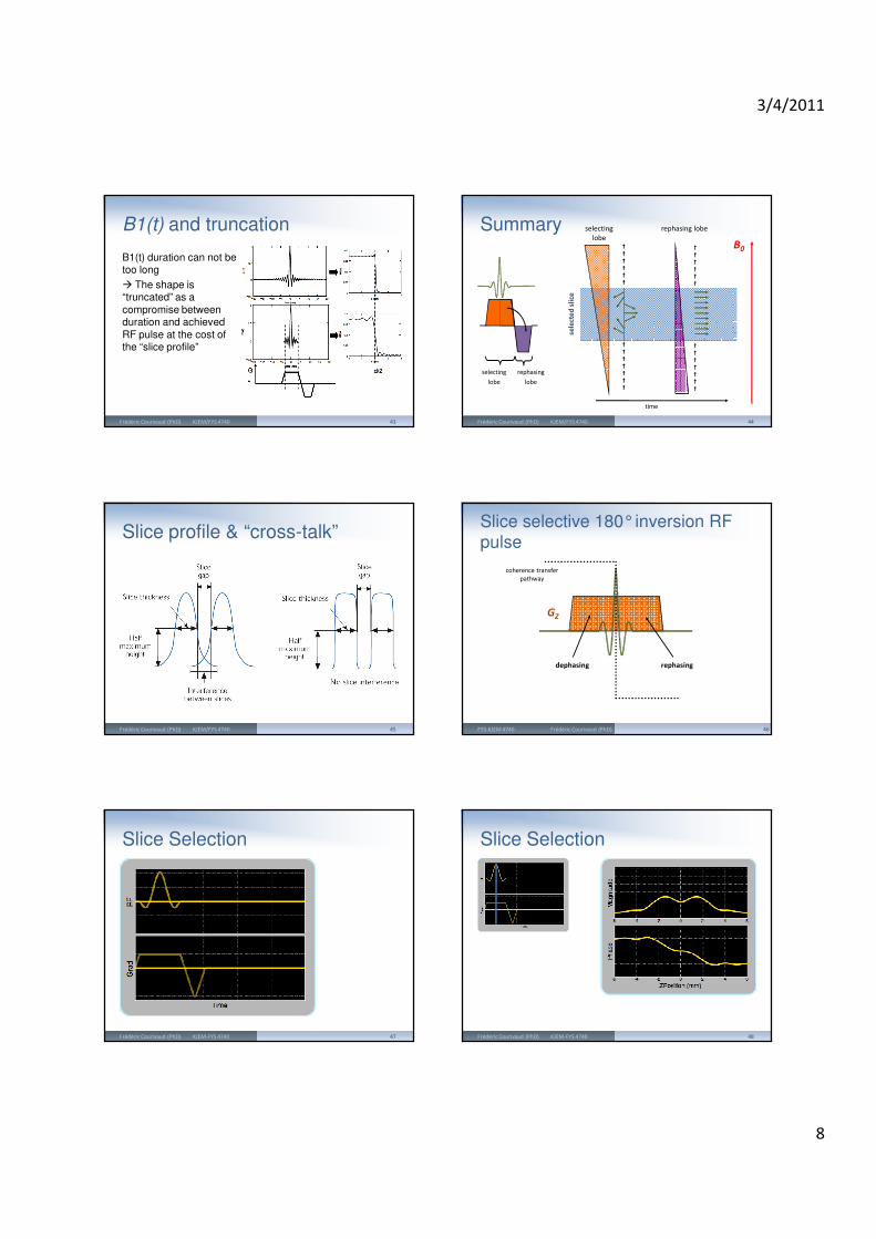
B1(t) and truncation

B1(t) duration can not be too long

The shape is “truncated” as a

compromise between duration and achieved

RF pulse at the cost of the “slice profile”


selecting

lobe

rephasing

lobe

B0

selecting

lobe

time

sele

cte

d s

lice

rephasing lobeSummary

44Frédéric Courivaud (PhD) KJEM/FYS 4740

Slice profile & “cross-talk”


coherence transfer

pathway

GZ

dephasing rephasing

Slice selective 180°inversion RF pulse


Slice Selection

Frédéric Courivaud (PhD) KJEM-FYS 4740 47

Slice Selection


3/4/2011

9

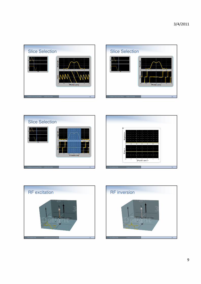
Slice Selection


Slice Selection


Slice Selection

Frédéric Courivaud (PhD) KJEM-FYS 4740 51 52FYS-KJEM 4740 Frédéric Courivaud (PhD)

RF excitation


RF inversion


3/4/2011

10

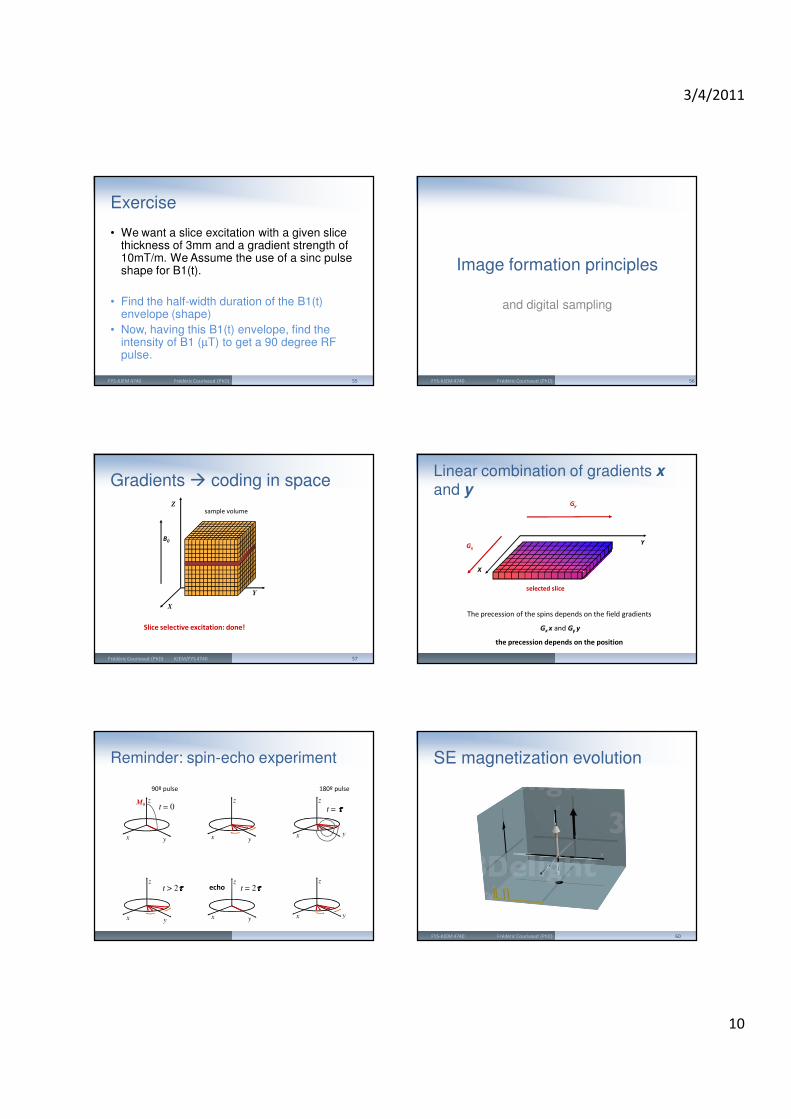
Exercise

• We want a slice excitation with a given slice thickness of 3mm and a gradient strength of 10mT/m. We Assume the use of a sinc pulse shape for B1(t).

• Find the half-width duration of the B1(t) envelope (shape)

• Now, having this B1(t) envelope, find the intensity of B1 (µT) to get a 90 degree RF pulse.


Image formation principles

and digital sampling


Z

X

Y

sample volume

B0

Slice selective excitation: done!

Gradients coding in space


selected slice

X

YGx

The precession of the spins depends on the field gradients

Gx x and Gy y

the precession depends on the position

Gy

Linear combination of gradients xand y

z

x y

z

x y

z

x y

echo t = 2ττττz

x y

t > 2ττττ

z

x y

M0 t = 0

90º pulse

z

x y

t = ττττ

180º pulse

Reminder: spin-echo experiment SE magnetization evolution


3/4/2011

11

Gy

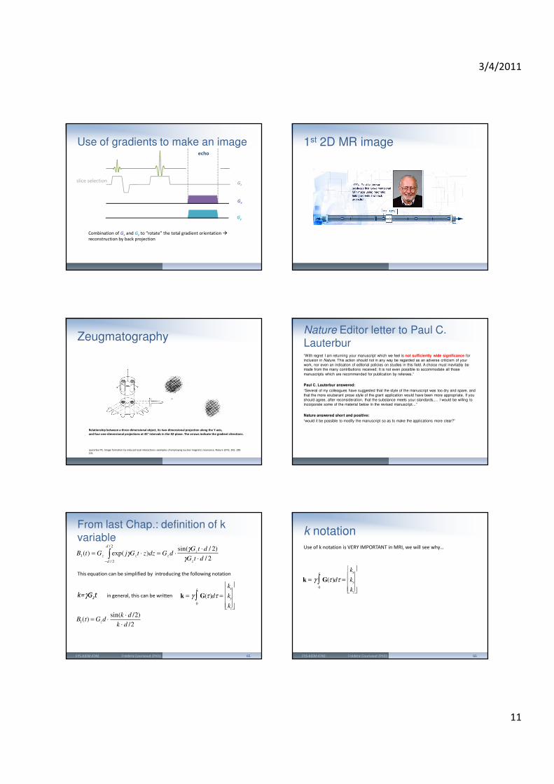
Combination of Gx and Gy to “rotate” the total gradient orientation

reconstruction by back projection

slice selectionGz

Gx

echo

Use of gradients to make an image 1st 2D MR image

Zeugmatography

Relationship between a three-dimensional object, its two-dimensional projection along the Y-axis,

and four one-dimensional projections at 45° intervals in the XZ-plane. The arrows indicate the gradient directions.

Lauterbur PC. Image formation by induced local interactions: examples of employing nuclear magnetic resonance. Nature 1973; 242: 190-

191.

Nature Editor letter to Paul C. Lauterbur“With regret I am returning your manuscript which we feel is not sufficiently wide significance for

inclusion in Nature. This action should not in any way be regarded as an adverse criticism of your

work, nor even an indication of editorial policies on studies in this field. A choice must inevitably be

made from the many contributions received; It is not even possible to accommodate all those

manuscripts which are recommended for publication by referees.”

Paul C. Lauterbur answered:

“Several of my colleagues have suggested that the style of the manuscript was too dry and spare, and

that the more exuberant prose style of the grant application would have been more appropriate. If you

should agree, after reconsideration, that the substance meets your standards,… I would be willing to

incorporate some of the material below in the revised manuscript…”

Nature answered short and positive:

“would it be possible to modify the manuscript so as to make the applications more clear?”

2/

)2/sin()exp()(

2/

2/

1dtG

dtGdGdzztGjGtB

z

z

z

d

d

zz⋅

⋅⋅=⋅= ∫

−γ

γγ

From last Chap.: definition of kvariable


This equation can be simplified by introducing the following notation

k=γGzt in general, this can be written

B1(t) = Gzd ⋅sin(k ⋅ d /2)

k ⋅ d /2

k = γ G(τ )0

t

∫ dτ =

kx

ky

kz

k notation


Use of k notation is VERY IMPORTANT in MRI, we will see why…

k = γ G(τ )0

t

∫ dτ =

kx

ky

kz

3/4/2011

12

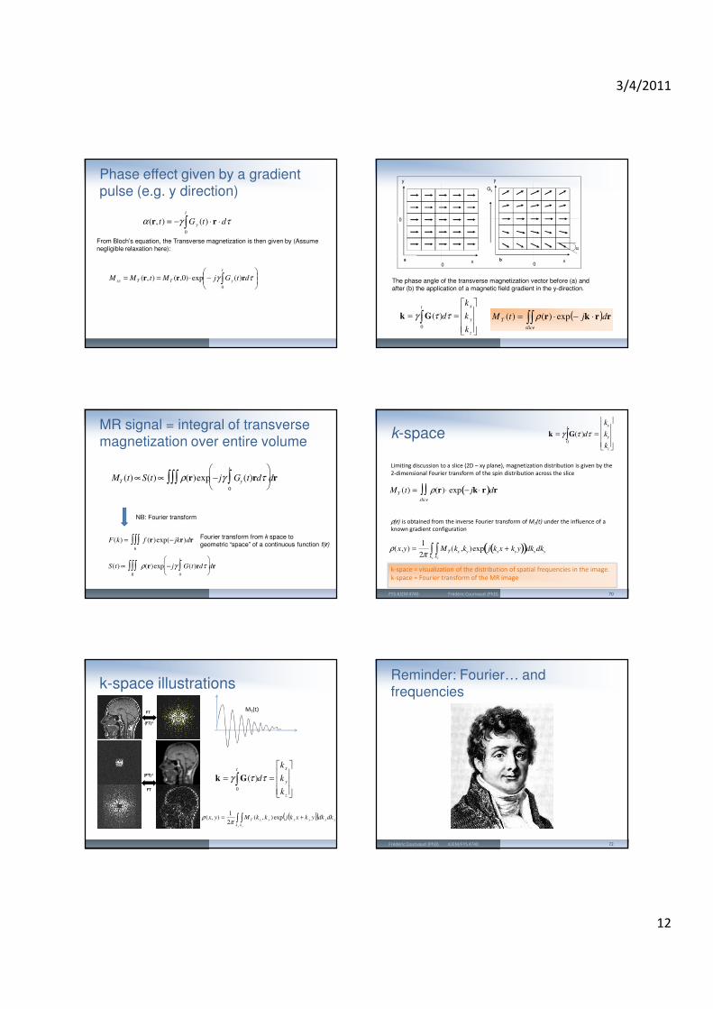
∫ ⋅⋅−=t

y dtGt0

)(),( τγα rr

From Bloch’s equation, the Transverse magnetization is then given by (Assume

negligible relaxation here):

−⋅== ∫

t

yTTxy dtGjMtMM0

)(exp)0,(),( τγ rrr

Phase effect given by a gradient pulse (e.g. y direction)

( )∫∫ ⋅−⋅=slice

T djtM rrkr exp)()( ρ

0

0

x

y y

0x

Gy

α

a b

The phase angle of the transverse magnetization vector before (a) and

after (b) the application of a magnetic field gradient in the y-direction.

== ∫z

y

xt

k

k

k

dττγ0

)(Gk

MT (t) ∝S(t) ∝ ρ(r)exp − jγ Gy(t)rdτ0

t

∫

∫∫∫ dr

F(k) = f (r)exp(− jkr)drR

∫∫∫

NB: Fourier transform

S(t) ∝ ρ(r)exp − jγ G(t)rdτ0

t

∫

R

∫∫∫ dr

MR signal = integral of transverse magnetization over entire volume

Fourier transform from k space to

geometric “space” of a continuous function f(r)

k-space


k = γ G(τ )0

t

∫ dτ =

kx

ky

kz

Limiting discussion to a slice (2D – xy plane), magnetization distribution is given by the

2-dimensional Fourier transform of the spin distribution across the slice

MT (t) = ρ(r)⋅ exp − jk⋅ r( )drslice

∫∫

ρ(r) is obtained from the inverse Fourier transform of MT(t) under the influence of a

known gradient configuration

ρ(x,y) =1

2πMT(kx ,ky )exp j kxx + kyy( )( )dkxdky

ky

∫kx

∫

k-space = visualization of the distribution of spatial frequencies in the image.

k-space = Fourier transform of the MR image

FT

FT-1

FT

FT-1

FT

FT-1

FT

FT-1

( )( )∫ ∫ +=

x yk k

yxyxyxT dkdkykxkjkkMyx exp),(2

1),(

πρ

MT(t)

== ∫z

y

xt

k

k

k

dττγ0

)(Gk

k-space illustrationsReminder: Fourier… and frequencies


3/4/2011

13

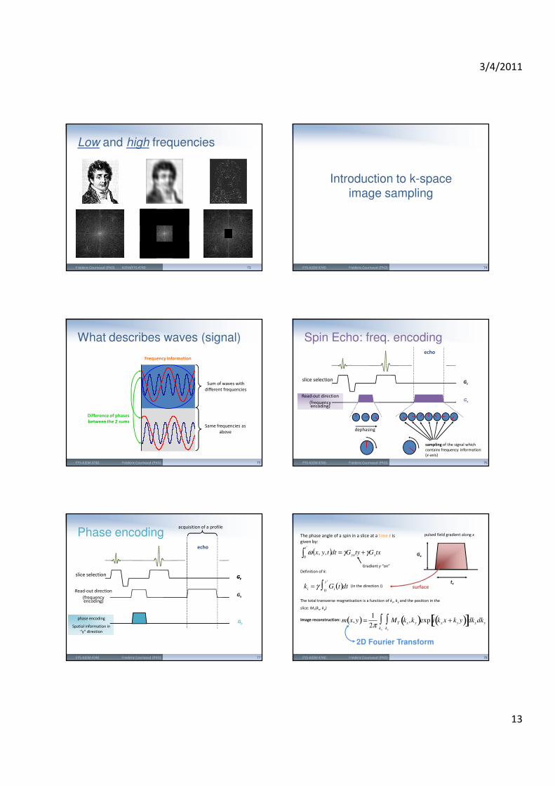
Low and high frequencies


Introduction to k-space image sampling


Sum of waves with

different frequencies

Frequency information

Difference of phases

between the 2 sumsSame frequencies as

above

What describes waves (signal)


dephasing

sampling of the signal which

contains frequency information

(x-axis)

Spin Echo: freq. encoding

slice selection

Read-out direction

(frequency encoding)

Gz

Gx

echo


phase encoding

Spatial information in

“y” direction

Gy

Phase encoding

Gzslice selection

Read-out direction


Gz

Gx

echo

acquisition of a profile


ki = γ Gi t( )0

′ t

∫ dt

The phase angle of a spin in a slice at a time t is

given by:

( ) txGtyGdttyxxyn

t

γγω +=∫′

0,,

Gradient y “on”

Definition of k:

pulsed field gradient along x

tx

Gx

(in the direction i) surface

The total transverse magnetisation is a function of kx, ky and the position in the

slice: MT(kx, ky)

Image reconstruction: m x,y( )=1

2πMT kx,ky( )exp i kx x + ky y( )[ ]dkxdky

ky

∫kx

∫

2D Fourier Transform


3/4/2011

14

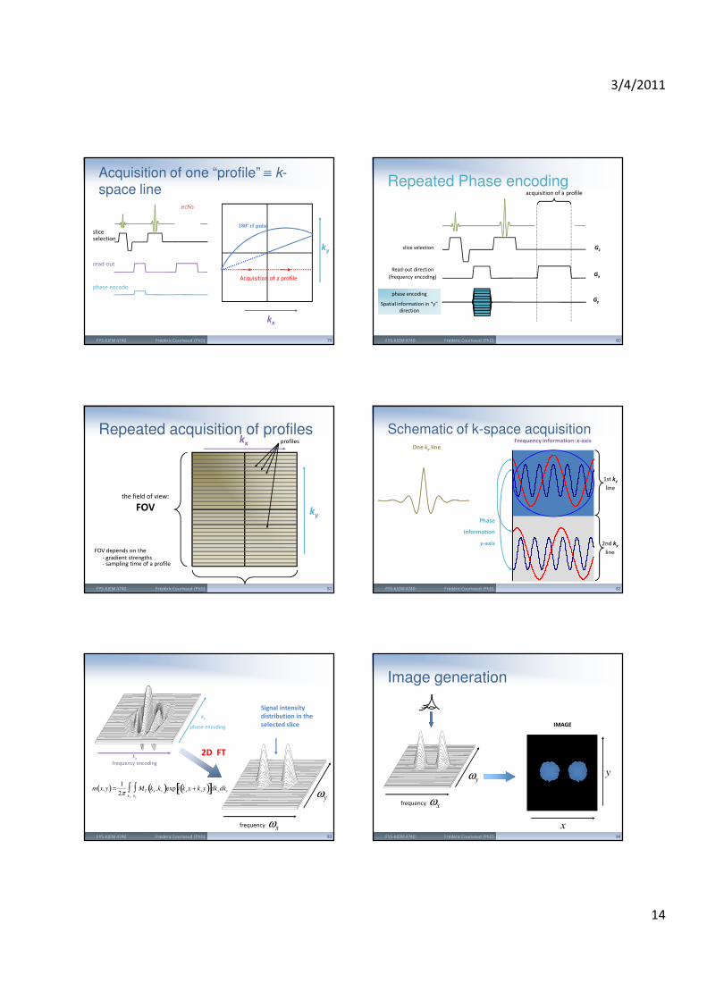
read-out

phase encode

sliceselection

180º rf pulse

kx

ky

echo

Acquisition of a profile

Acquisition of one “profile” ≡ k-space line


slice selection

Read-out direction


phase encoding

Spatial information in “y”

direction

Gz

Gx

Gy

acquisition of a profile

Repeated Phase encoding


Repeated acquisition of profiles

ky

kx

the field of view:

FOV

profiles

FOV depends on the

- gradient strengths- sampling time of a profile


One ky line

1st ky

line

Frequency information: x-axis

Phase

information

y-axis 2nd ky

line

Schematic of k-space acquisition


kx

frequency encoding

ky

phase encoding

2D FT

Signal intensity

distribution in the

selected slice

frequency ωx

ωy

m x, y( )=1

2πMT kx ,ky( )exp i kx x + ky y( )[ ]dkxdky

ky

∫kx

∫


frequency ωx

ωy

IMAGE

x

y

Image generation


3/4/2011

15

CONTINUE PPT FROM HERE


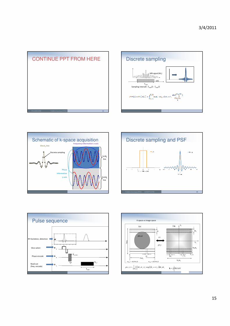
Sampling intervall: -Tread/2 - Tread/2

Tread

U(t)

MR-signal (MT)

Discrete sampling

One ky line

Discrete sampling

1st ky

line

Frequency information: x-axis

Phase

information

y-axis 2nd ky

line

Schematic of k-space acquisition Discrete sampling and PSF


Pulse sequence

0 20 40 60 80 100 120 140

0.5

0

0.5

1

time (ms)

B1

(t)

RF

Gz

Gy

Gx

0 20 40 60 80 100 120 140

0.5

0

0.5

1

time (ms)

B1

(t)

RF

Gz

Gy

Gx

0 20 40 60 80 100 120 140

0.5

0

0.5

1

time (ms)

B1

(t)

RF

Gz

Gy

Gx

Slice-select

Phase-encode

Read-out

(freq. encode)

RF-Excitation, detection

Tread

Ty

Gy_max

Gx_r

FT

FT-1

∆x ∆kx

F(k)S(r)

FoVx

FoV

y

∆y ∆ky

Nx∆kx

Ny∆ky

ts

ky

kx

-ωmax = -γGxFoVx/2 ωmax = γGxFoVx/2

.ρ(x,y)

kx_max

K-space vs image space

( )( )∫ ∫ +=

x yk k

yxyxyxT dkdkykxkjkkMyx exp),(2

1),(

πρ

== ∫z

y

xt

k

k

k

dττγ0

)(Gk

3/4/2011

16

K-space egenskaper

sxx tNGx

γ

πδ

2=

Resolution (x):

Field of view (x):

x

sxx

x FoVtGk

===γ

ππλ

22

min,

max,

Field of view (y):

yy

y

yyTG

NFoV

max_

max,γ

πλ ==

Maximum frequency in read-out (x) direction

2/max xx FoVGγω ±=±

πγ 2//1 xxs FoVGt ≥

Min sampling rate (x):

yyyyFoVTGN

max_γ=

‘Sampling rate ‘ (y):

Image F

oV

y

Obje

ct F

oV

y

Object FoV

Image FoV

Increase 1/ts, Nx

discardeddiscarded

FFT 1D: Truncation Artefact


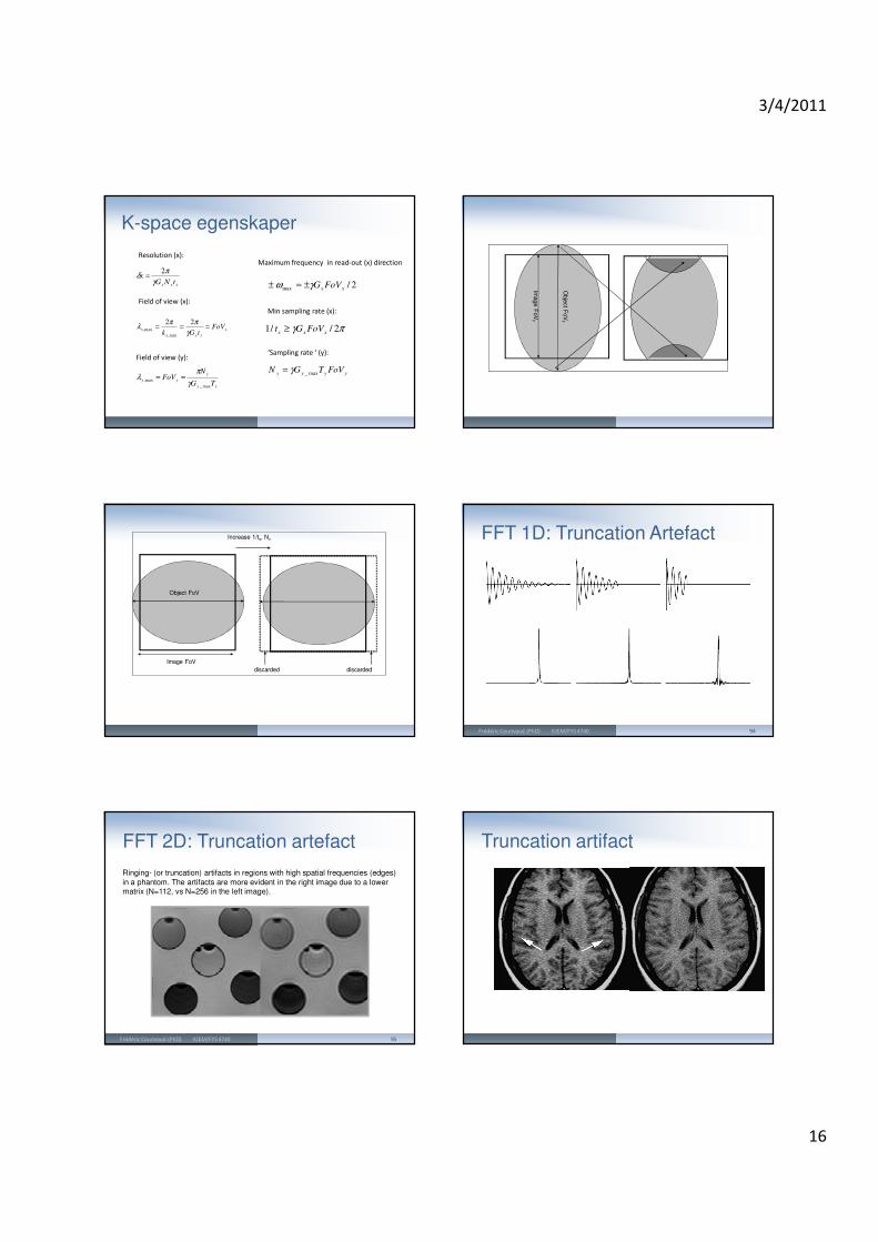
FFT 2D: Truncation artefact

Ringing- (or truncation) artifacts in regions with high spatial frequencies (edges)

in a phantom. The artifacts are more evident in the right image due to a lower matrix (N=112, vs N=256 in the left image).


Truncation artifact

3/4/2011

17


slice selectionGz

Gx

echo

K-space sampling principles

Gy

Combination of Gx and Gy to “rotate” the total gradient orientation

reconstruction by back projection

slice selectionGz

Gx

echo

z

x y

z

x y

z

x y

echo

z

x y

z

x y

M

0

90º pulse

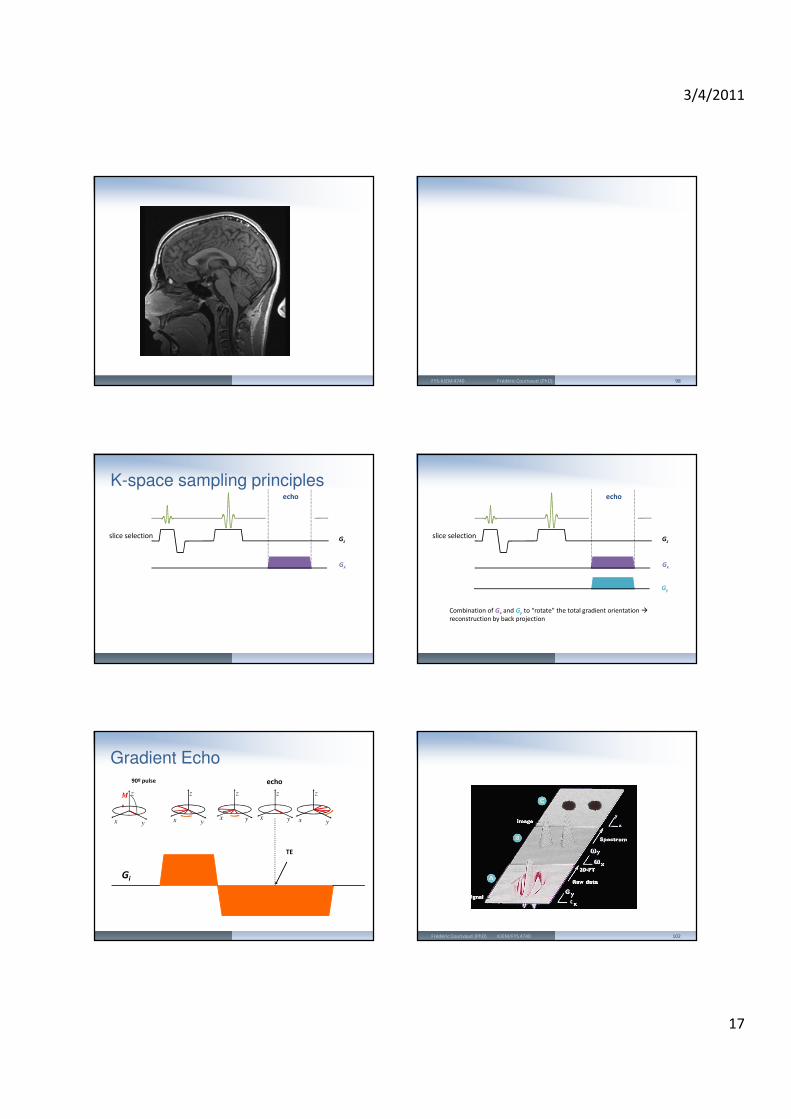
Gi

TE

Gradient Echo


3/4/2011

18

103FYS-KJEM 4740 Frédéric Courivaud (PhD) 104FYS-KJEM 4740 Frédéric Courivaud (PhD)

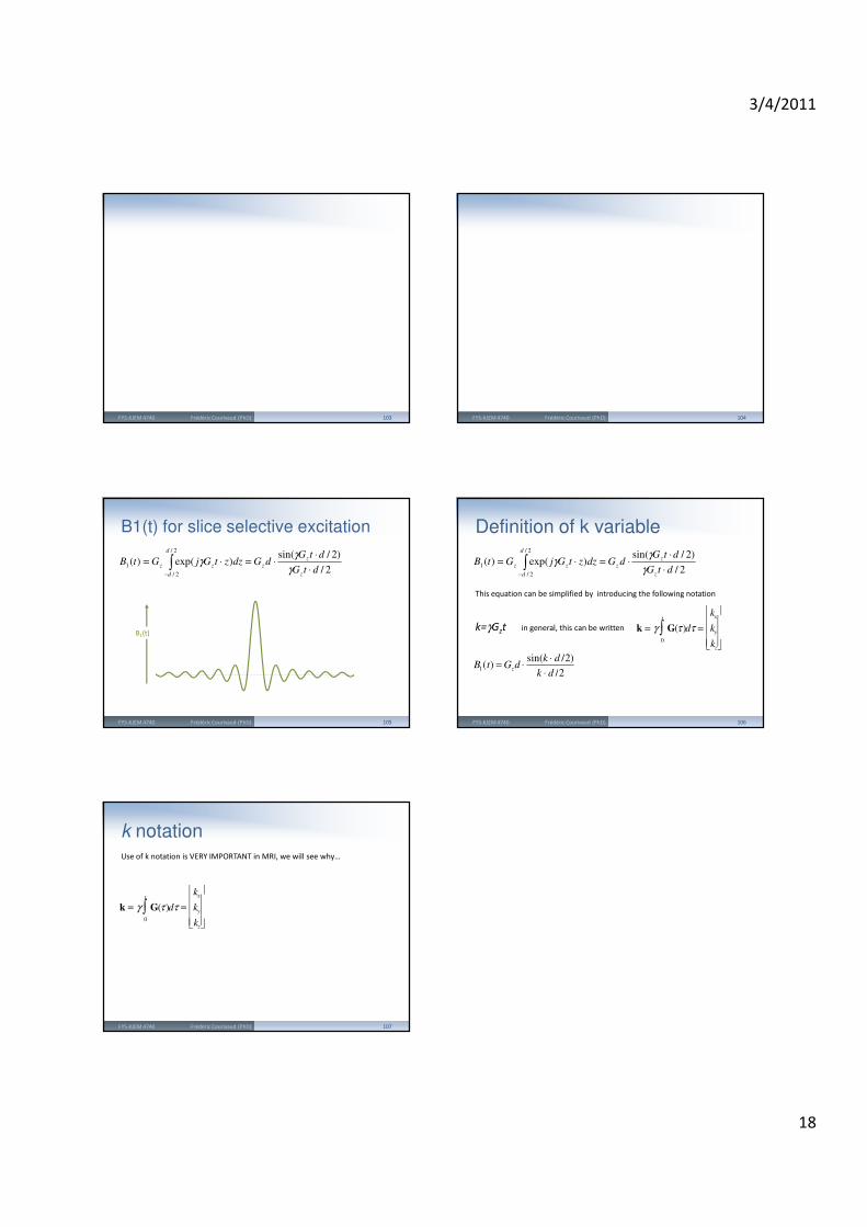
2/

)2/sin()exp()(

2/

2/

1dtG

dtGdGdzztGjGtB

z

z

z

d

d

zz⋅

⋅⋅=⋅= ∫

−γ

γγ

B1(t) for slice selective excitation


B1(t)

2/

)2/sin()exp()(

2/

2/

1dtG

dtGdGdzztGjGtB

z

z

z

d

d

zz⋅

⋅⋅=⋅= ∫

−γ

γγ

Definition of k variable


This equation can be simplified by introducing the following notation

k=γGzt in general, this can be written

B1(t) = Gzd ⋅sin(k ⋅ d /2)

k ⋅ d /2

k = γ G(τ )0

t

∫ dτ =

kx

ky

kz

k notation


Use of k notation is VERY IMPORTANT in MRI, we will see why…

k = γ G(τ )0

t

∫ dτ =

kx

ky

kz

FYS-KJM 4740 Chap1-2...FYS-KJM 4740 Chap 1 Bloch equations and main principles FYS-KJEM 4740...

Documents

Transcript of FYS-KJM 4740 Chap1-2...FYS-KJM 4740 Chap 1 Bloch equations and main principles FYS-KJEM 4740...