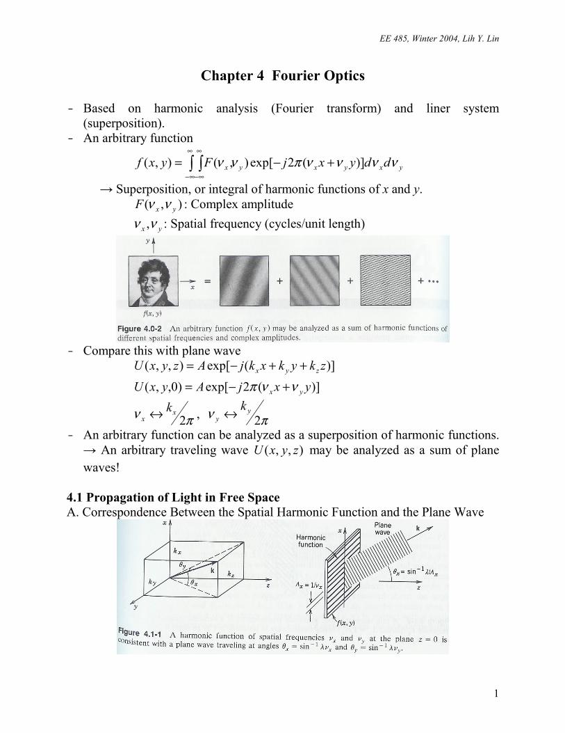
EE 485, Winter 2004, Lih Y. Lin

1

Chapter 4 Fourier Optics

- Based on harmonic analysis (Fourier transform) and liner system (superposition).

- An arbitrary function

yxyxyx ddyxjFyxf ννννπνν )](2exp[),(),( +−= ∫ ∫∞

∞−

∞

∞−

→ Superposition, or integral of harmonic functions of x and y. ),( yxF νν : Complex amplitude yx νν , : Spatial frequency (cycles/unit length)

- Compare this with plane wave

)](2exp[)0,,()](exp[),,(

yxjAyxUzkykxkjAzyxU

yx

zyx

ννπ +−=

++−=

πνπν 2 , 2y

yx

xkk ↔↔

- An arbitrary function can be analyzed as a superposition of harmonic functions. → An arbitrary traveling wave ),,( zyxU may be analyzed as a sum of plane waves!

4.1 Propagation of Light in Free Space A. Correspondence Between the Spatial Harmonic Function and the Plane Wave

EE 485, Winter 2004, Lih Y. Lin

2

)(sinsin

)(sinsin

11

11

yy

y

xx

x

kk

kk

λνθ

λνθ

−−

−−

=

=

=

=

(4.1-1)

A physical way of picturing the spatial harmonic function is to project a plane wave on the x-y plane.

yy

xx νν

1 ,1 =Λ=Λ

→

Λ=

Λ= −−

yy

xx

λθλθ 11 sin ,sin

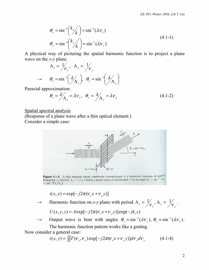
Paraxial approximation: yx , λνλθλνλθ =Λ==Λ=

yy

xx (4.1-2)

Spatial spectral analysis (Response of a plane wave after a thin optical element.) Consider a simple case:

)](2exp[),( yxjyxt yx ννπ +−=

→ Harmonic function on x-y plane with period y

yx

x νν1 ,1 =Λ=Λ .

)exp()](2exp[),,( zjkyxjAzyxU zyx −+−= ννπ → Output wave is bent with angles )(sin ),(sin 11

yyxx λνθλνθ −− == . The harmonic function pattern works like a grating.

Now consider a general case: yxyxyx ddyxjFyxt ννννπνν )](2exp[),(),( +−= ∫∫ (4.1-4)

EE 485, Winter 2004, Lih Y. Lin

3

yxzyxyx ddzjkyxjFzyxU ννννπνν )exp()](2exp[),(),,( −+−= ∫∫

222222 1112

yxyxz kkkk

λλλπ −−=−−=

→ An incident plane wave is decomposed into many plane waves, each traveling at angles )(sin ),(sin 11

yyxx λνθλνθ −− == , with a complex envelope ),( yxF νν , the Fourier transform of ),( yxf .

Example 4.1-2, Imaging

( )

fxyx

yxjfxjyxt

λϕ

πϕλπ

2),(

),(2expexp),(

2

2

−=

−=

=

Compare to earlier: yxyx yx ννϕ +↔),(

Now fx

xyxx xx λ

ϕνν −=∂

∂=⇒),( with varies

−=⇒ −

fx

x1sinθ

→ A cylindrical lens with focal length f

EE 485, Winter 2004, Lih Y. Lin

4

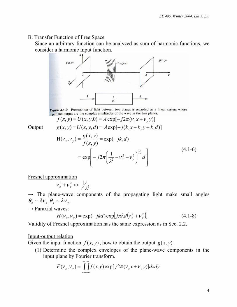
B. Transfer Function of Free Space

Since an arbitrary function can be analyzed as sum of harmonic functions, we consider a harmonic input function.

)](2exp[)0,,(),( yxjAyxUyxf yx ννπ +−== Output )](exp[),,(),( dkykxkjAdyxUyxg zyx ++−==

−−−=

−==Η

dj

djkyxfyxg

yx

zyx

21

222

12exp

)exp(),(),(),(

ννλ

π

νν

(4.1-6)

Fresnel approximation 2

22 1λνν <<+ yx

→ The plane-wave components of the propagating light make small angles yyxx λνθλνθ ~,~ .

→ Paraxial waves: ( )[ ]22exp)exp(),( yxyx djjkdH ννπλνν +−= (4.1-8) Validity of Fresnel approximation has the same expression as in Sec. 2.2. Input-output relation Given the input function ),( yxf , how to obtain the output ),( yxg :

(1) Determine the complex envelopes of the plane-wave components in the input plane by Fourier transform.

dxdyyxjyxfF yxyx )](2exp[),(),( ννπνν += ∫ ∫∞

∞−

∞

∞−

EE 485, Winter 2004, Lih Y. Lin

5

(2) Complex envelopes of the plane-wave components in the output plane = ),(),( yxyx FH νννν (3) yxyxyxyx ddyxjFHyxg ννννπνννν )](2exp[),(),(),( +−= ∫∫ Under Fresnel approximation,

)exp(

)](2exp[)](exp[),(),(

0

220

jkdHddyxjdjFHyxg yxyxyxyx

−≡

+−+= ∫∫ ννννπννπλνν

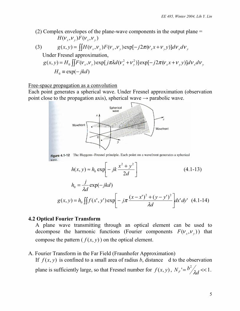
Free-space propagation as a convolution Each point generates a spherical wave. Under Fresnel approximation (observation point close to the propagation axis), spherical wave → parabolic wave.

+−≈d

yxjkhyxh2

exp),(22

0 (4.1-13)

)exp(0 jkddjh −=

λ

'')'()'(exp)','(),(22

0 dydxd

yyxxjyxfhyxg ∫∫

−+−−=λ

π (4.1-14)

4.2 Optical Fourier Transform

A plane wave transmitting through an optical element can be used to decompose the harmonic functions (Fourier components ),( yxF νν ) that compose the pattern ( ),( yxf ) on the optical element.

A. Fourier Transform in the Far Field (Fraunhofer Approximation)

If ),( yxf is confined to a small area of radius b, distance d to the observation

plane is sufficiently large, so that Fresnel number for ),( yxf , 1'2

<<= dbNF λ .

EE 485, Winter 2004, Lih Y. Lin

6

),(exp),(22

0 dy

dxF

dyxjhyxg

λλλπ

+−= (4.2-4)

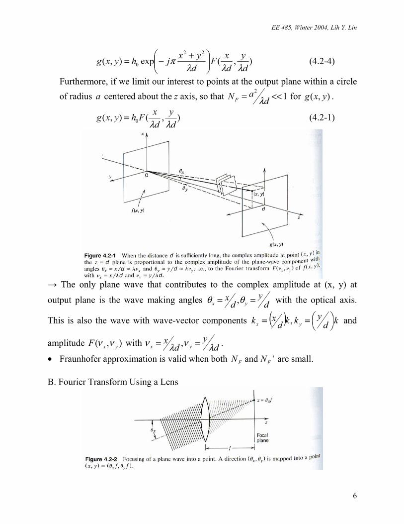
Furthermore, if we limit our interest to points at the output plane within a circle of radius a centered about the z axis, so that 1

2<<= d

aNF λ for ),( yxg .

),(),( 0 dy

dxFhyxg

λλ= (4.2-1)

→ The only plane wave that contributes to the complex amplitude at (x, y) at

output plane is the wave making angles dy

dx

yx == θθ , with the optical axis.

This is also the wave with wave-vector components ( ) kdykkd

xk yx

== , and

amplitude ),( yxF νν with dy

dx

yx λνλν == , .

• Fraunhofer approximation is valid when both ' and FF NN are small. B. Fourier Transform Using a Lens

EE 485, Winter 2004, Lih Y. Lin

7

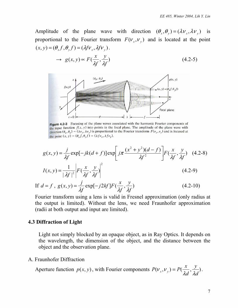
Amplitude of the plane wave with direction ),(),( yxyx λνλνθθ = is proportional to the Fourier transform ),( yxF νν and is located at the point

),(),(),( yxyx ffffyx νλνλθθ == .

→ ),(),(fy

fxFyxg

λλ∝ (4.2-5)

),())((exp)](exp[),( 2

22

fy

fxF

ffdyxjfdjk

fjyxg

λλλπ

λ

−++−= (4.2-8)

2

2 ),(||

1),(fy

fxF

fyxI

λλλ= (4.2-9)

If fd = , ),(]2exp[),(fy

fxFkfj

fjyxg

λλλ−= (4.2-10)

Fourier transform using a lens is valid in Fresnel approximation (only radius at the output is limited). Without the lens, we need Fraunhofer approximation (radii at both output and input are limited).

4.3 Diffraction of Light

Light not simply blocked by an opaque object, as in Ray Optics. It depends on the wavelength, the dimension of the object, and the distance between the object and the observation plane.

A. Fraunhofer Diffraction

Aperture function ),( yxp , with Fourier components ),(),(dy

dxPP yx λλ

νν = .

EE 485, Winter 2004, Lih Y. Lin

8

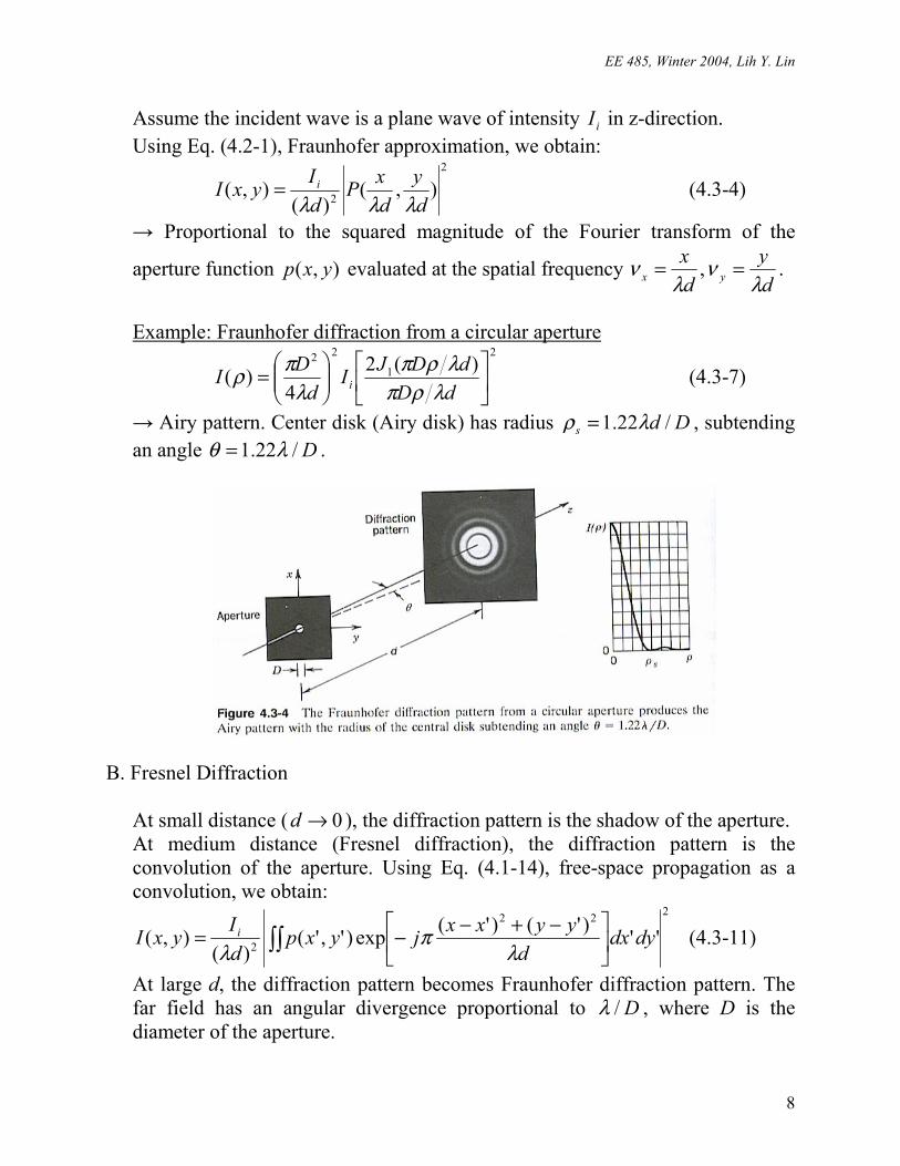
Assume the incident wave is a plane wave of intensity iI in z-direction. Using Eq. (4.2-1), Fraunhofer approximation, we obtain:

2

2 ),()(

),(dy

dxP

dIyxI i

λλλ= (4.3-4)

→ Proportional to the squared magnitude of the Fourier transform of the

aperture function ),( yxp evaluated at the spatial frequency dy

dx

yx λν

λν == , .

Example: Fraunhofer diffraction from a circular aperture

2

1

22 )(24

)(

=

dDdDJI

dDI i λρπ

λρπλ

πρ (4.3-7)

→ Airy pattern. Center disk (Airy disk) has radius Dds /22.1 λρ = , subtending an angle D/22.1 λθ = .

B. Fresnel Diffraction

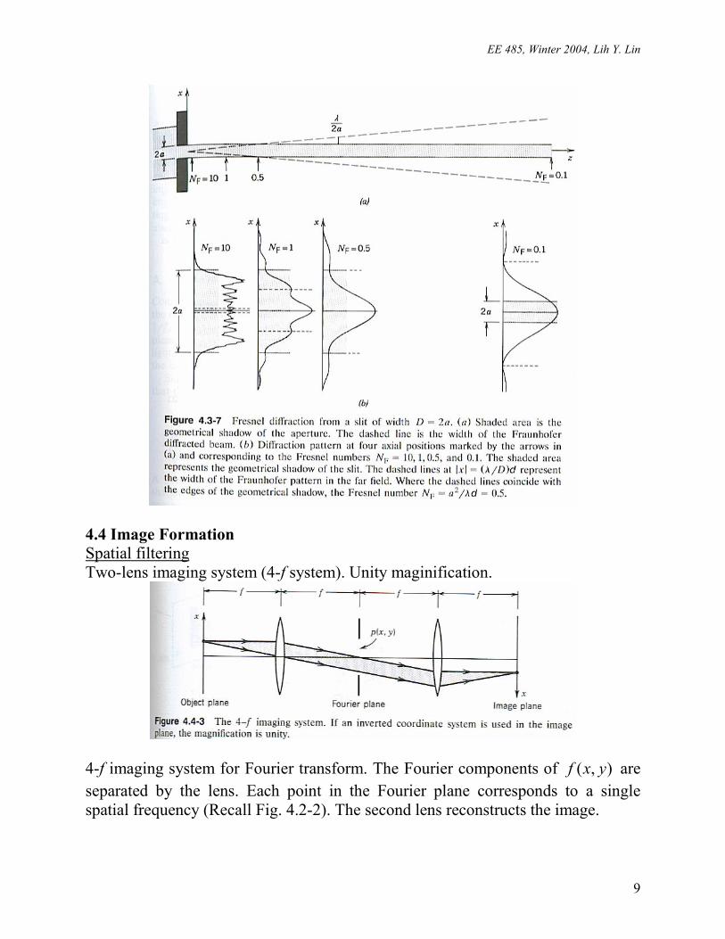
At small distance ( 0→d ), the diffraction pattern is the shadow of the aperture. At medium distance (Fresnel diffraction), the diffraction pattern is the convolution of the aperture. Using Eq. (4.1-14), free-space propagation as a convolution, we obtain:

222

2 '')'()'(exp)','()(

),( ∫∫

−+−−= dydxd

yyxxjyxpdIyxI i

λπ

λ (4.3-11)

At large d, the diffraction pattern becomes Fraunhofer diffraction pattern. The far field has an angular divergence proportional to D/λ , where D is the diameter of the aperture.

EE 485, Winter 2004, Lih Y. Lin

9

4.4 Image Formation Spatial filtering Two-lens imaging system (4-f system). Unity maginification.

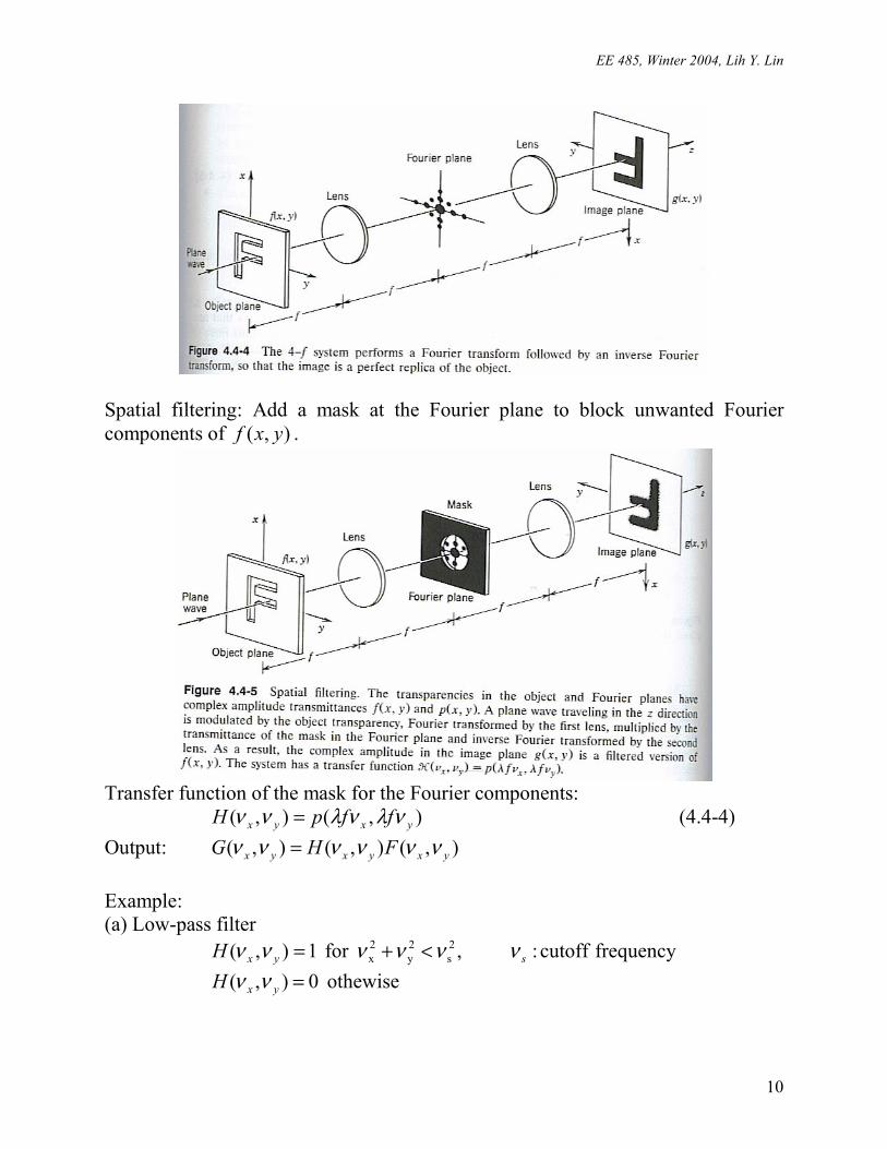
4-f imaging system for Fourier transform. The Fourier components of ),( yxf are separated by the lens. Each point in the Fourier plane corresponds to a single spatial frequency (Recall Fig. 4.2-2). The second lens reconstructs the image.

EE 485, Winter 2004, Lih Y. Lin

10

Spatial filtering: Add a mask at the Fourier plane to block unwanted Fourier components of ),( yxf .

Transfer function of the mask for the Fourier components: ),(),( yxyx ffpH νλνλνν = (4.4-4) Output: ),(),(),( yxyxyx FHG νννννν = Example: (a) Low-pass filter frequency cutoff : ,for 1),( 2

s2y

2x syxH νννννν <+=

othewise 0),( =yxH νν

EE 485, Winter 2004, Lih Y. Lin

11

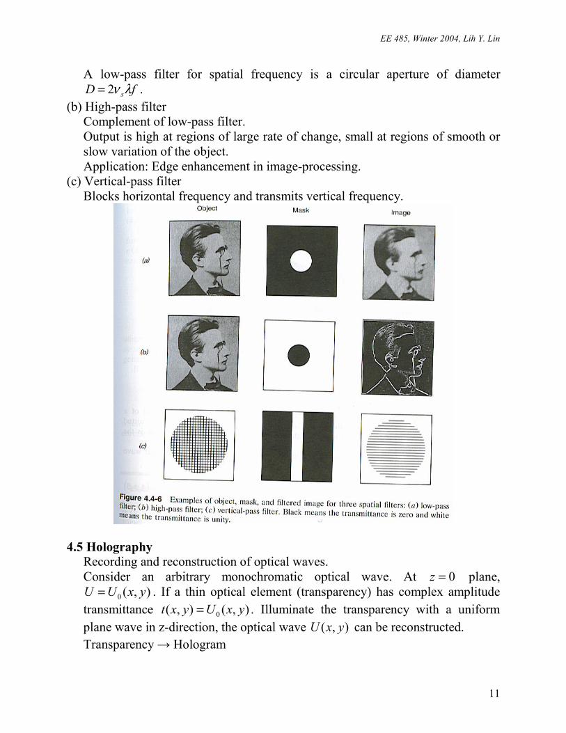
A low-pass filter for spatial frequency is a circular aperture of diameter fD sλν2= .

(b) High-pass filter Complement of low-pass filter. Output is high at regions of large rate of change, small at regions of smooth or slow variation of the object. Application: Edge enhancement in image-processing.

(c) Vertical-pass filter Blocks horizontal frequency and transmits vertical frequency.

4.5 Holography Recording and reconstruction of optical waves. Consider an arbitrary monochromatic optical wave. At 0=z plane,

),(0 yxUU = . If a thin optical element (transparency) has complex amplitude transmittance ),(),( 0 yxUyxt = . Illuminate the transparency with a uniform plane wave in z-direction, the optical wave ),( yxU can be reconstructed. Transparency → Hologram

EE 485, Winter 2004, Lih Y. Lin

12

How to get ),( yxt from ),(0 yxU ? Phase information is very important. Need some kind of coding to transform phase into intensity.

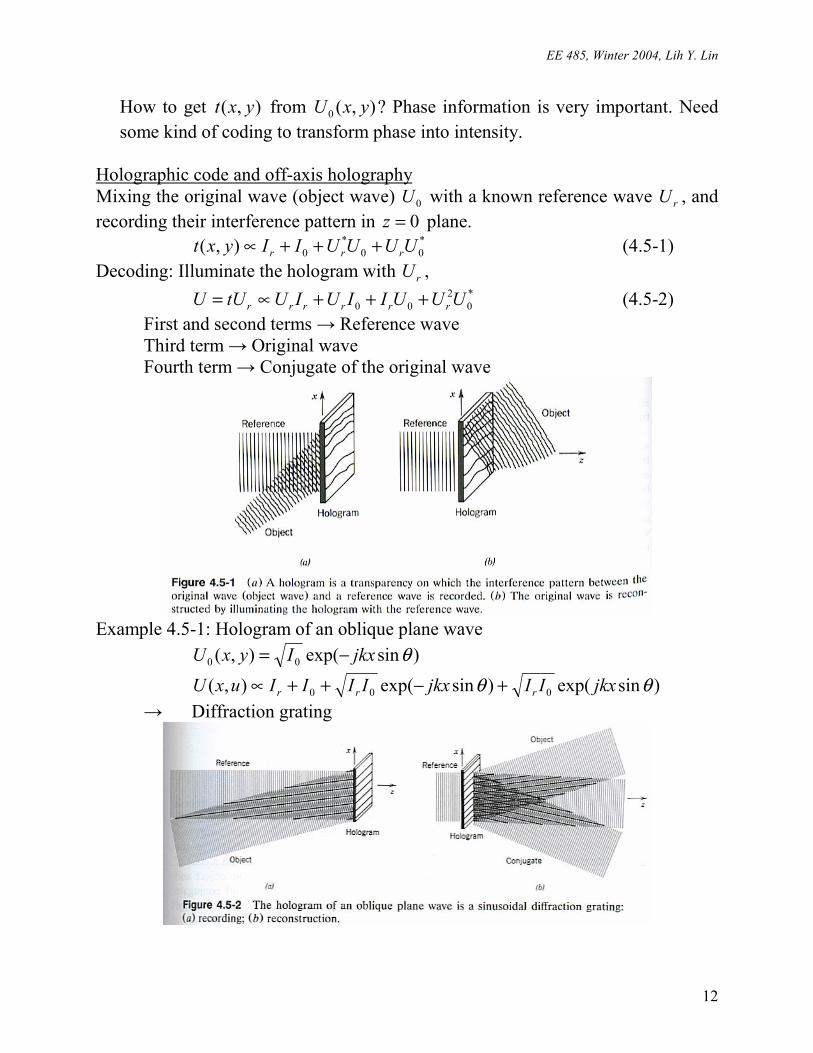
Holographic code and off-axis holography Mixing the original wave (object wave) 0U with a known reference wave rU , and recording their interference pattern in 0=z plane. *

00*

0),( UUUUIIyxt rrr +++∝ (4.5-1) Decoding: Illuminate the hologram with rU , *

02

00 UUUIIUIUtUU rrrrrr +++∝= (4.5-2) First and second terms → Reference wave Third term → Original wave Fourth term → Conjugate of the original wave

Example 4.5-1: Hologram of an oblique plane wave )sinexp(),( 00 θjkxIyxU −= )sinexp()sinexp(),( 000 θθ jkxIIjkxIIIIuxU rrr +−++∝ → Diffraction grating

EE 485, Winter 2004, Lih Y. Lin

13

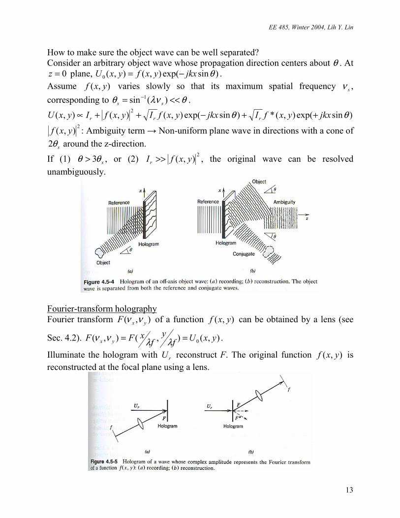
How to make sure the object wave can be well separated? Consider an arbitrary object wave whose propagation direction centers about θ . At

0=z plane, )sinexp(),(),(0 θjkxyxfyxU −= . Assume ),( yxf varies slowly so that its maximum spatial frequency sν , corresponding to θλνθ <<= − )(sin 1

ss . )sinexp(),(*)sinexp(),(),(),( 2 θθ jkxyxfIjkxyxfIyxfIyxU rrr ++−++∝

2),( yxf : Ambiguity term → Non-uniform plane wave in directions with a cone of

sθ2 around the z-direction.

If (1) xθθ 3> , or (2) 2),( yxfIr >> , the original wave can be resolved unambiguously.

Fourier-transform holography Fourier transform ),( yxF νν of a function ),( yxf can be obtained by a lens (see

Sec. 4.2). ),(),(),( 0 yxUfy

fxFF yx == λλνν .

Illuminate the hologram with rU reconstruct F. The original function ),( yxf is reconstructed at the focal plane using a lens.

EE 485, Winter 2004, Lih Y. Lin

14

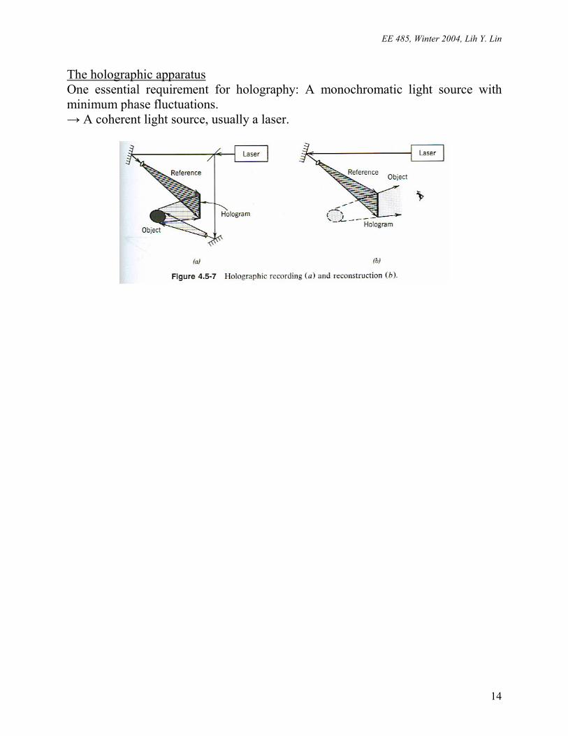
The holographic apparatus One essential requirement for holography: A monochromatic light source with minimum phase fluctuations. → A coherent light source, usually a laser.