Local- and regional-scale measurements of CH4, δ13CH4, and ...
21
Atmos. Meas. Tech., 8, 4539–4559, 2015 www.atmos-meas-tech.net/8/4539/2015/ doi:10.5194/amt-8-4539-2015 © Author(s) 2015. CC Attribution 3.0 License. Local- and regional-scale measurements of CH 4 , δ 13 CH 4 , and C 2 H 6 in the Uintah Basin using a mobile stable isotope analyzer C. W. Rella, J. Hoffnagle, Y. He, and S. Tajima Picarro, Inc., 3105 Patrick Henry Drive, Santa Clara 95054, CA, USA Correspondence to: C. W. Rella ([email protected]) Received: 19 February 2015 – Published in Atmos. Meas. Tech. Discuss.: 13 May 2015 Revised: 28 September 2015 – Accepted: 4 October 2015 – Published: 30 October 2015 Abstract. In this paper, we present an innovative CH 4 , δ 13 CH 4 , and C 2 H 6 instrument based on cavity ring-down spectroscopy (CRDS). The design and performance of the analyzer is presented in detail. The instrument is capable of precision of less than 1 ‰ on δ 13 CH 4 with 1 in. of averag- ing and about 0.1 ‰ in an hour. Using this instrument, we present a comprehensive approach to atmospheric methane emissions attribution. Field measurements were performed in the Uintah Basin (Utah, USA) in the winter of 2013, us- ing a mobile lab equipped with the CRDS analyzer, a high- accuracy GPS, a sonic anemometer, and an onboard gas stor- age and playback system. With a small population and almost no other sources of methane and ethane other than oil and gas extraction activities, the Uintah Basin represents an ideal lo- cation to investigate and validate new measurement methods of atmospheric methane and ethane. We present the results of measurements of the individual fugitive emissions from 23 natural gas wells and six oil wells in the region. The δ 13 CH 4 and C 2 H 6 signatures that we observe are consistent with the signatures of the gases found in the wells. Furthermore, re- gional measurements of the atmospheric CH 4 , δ 13 CH 4 , and C 2 H 6 signatures throughout the basin have been made, using continuous sampling into a 450 m long tube and laboratory reanalysis with the CRDS instrument. These measurements suggest that 85 ± 7 % of the total emissions in the basin are from natural gas production. 1 Introduction The advent of the techniques of directional drilling, horizon- tal drilling, 3-D seismic imaging, and hydraulic fracturing have led to rapid increases in oil and gas production through- out the US, especially in basins where production using so- called conventional methods of extraction was not economi- cally viable. Together with the increase of oil and gas produc- tion, there has been a concurrent increase in gaseous emis- sions into the atmosphere. Methane, the primary constituent of natural gas, is a potent greenhouse gas with a global warm- ing potential of up to 86 times that of an equivalent mass of carbon dioxide over a 20-year timescale. With a moder- ate atmospheric lifetime of 12.4 years, the relative impact of methane on a 100-year timescale is 28 (Myhre et al., 2013). When emissions are kept under control, methane is a clean- burning, high energy content fuel that can reduce carbon dioxide emissions relative to other more carbon-rich fuels. However, when methane emissions are a relatively large frac- tion of total natural gas production, the climate benefit of nat- ural gas relative to coal (a relatively carbon-intensive fuel) is reduced or even eliminated (Alvarez et al., 2012). Several recent atmospheric studies using the aircraft mass- balance approach have focused on quantifying regional emis- sions from oil and gas production. In Pétron et al. (2014), the mass-balance approach using aircraft was used to quantify emissions in the Denver–Julesburg Basin in Colorado, deter- mining that the methane emissions from fossil fuel extraction activities are about 4 % of total natural gas production in the basin. This emission rate is in excess of both the inventory (Pétron et al., 2012) and the ∼ 3 % threshold where there are immediate climate benefits of switching from coal to natural gas electricity production (Alvarez et al., 2012). In the Uintah Basin in Utah, again using aircraft, Karion et al. (2013) re- ported methane emissions (February, 2012) to be 6.2–11.7 % of average daily production from the basin, again exceeding the inventory and the threshold for immediate climate bene- Published by Copernicus Publications on behalf of the European Geosciences Union.
Transcript of Local- and regional-scale measurements of CH4, δ13CH4, and ...
Atmos. Meas. Tech., 8, 4539–4559, 2015
www.atmos-meas-tech.net/8/4539/2015/
doi:10.5194/amt-8-4539-2015
© Author(s) 2015. CC Attribution 3.0 License.
Local- and regional-scale measurements of CH4, δ13CH4, and C2H6
in the Uintah Basin using a mobile stable isotope analyzer
C. W. Rella, J. Hoffnagle, Y. He, and S. Tajima
Picarro, Inc., 3105 Patrick Henry Drive, Santa Clara 95054, CA, USA
Correspondence to: C. W. Rella ([email protected])
Received: 19 February 2015 – Published in Atmos. Meas. Tech. Discuss.: 13 May 2015
Revised: 28 September 2015 – Accepted: 4 October 2015 – Published: 30 October 2015
Abstract. In this paper, we present an innovative CH4,
δ13CH4, and C2H6 instrument based on cavity ring-down
spectroscopy (CRDS). The design and performance of the
analyzer is presented in detail. The instrument is capable of
precision of less than 1 ‰ on δ13CH4 with 1 in. of averag-
ing and about 0.1 ‰ in an hour. Using this instrument, we
present a comprehensive approach to atmospheric methane
emissions attribution. Field measurements were performed
in the Uintah Basin (Utah, USA) in the winter of 2013, us-
ing a mobile lab equipped with the CRDS analyzer, a high-
accuracy GPS, a sonic anemometer, and an onboard gas stor-
age and playback system. With a small population and almost
no other sources of methane and ethane other than oil and gas
extraction activities, the Uintah Basin represents an ideal lo-
cation to investigate and validate new measurement methods
of atmospheric methane and ethane. We present the results of
measurements of the individual fugitive emissions from 23
natural gas wells and six oil wells in the region. The δ13CH4
and C2H6 signatures that we observe are consistent with the
signatures of the gases found in the wells. Furthermore, re-
gional measurements of the atmospheric CH4, δ13CH4, and
C2H6 signatures throughout the basin have been made, using
continuous sampling into a 450 m long tube and laboratory
reanalysis with the CRDS instrument. These measurements
suggest that 85± 7 % of the total emissions in the basin are
from natural gas production.
1 Introduction
The advent of the techniques of directional drilling, horizon-
tal drilling, 3-D seismic imaging, and hydraulic fracturing
have led to rapid increases in oil and gas production through-
out the US, especially in basins where production using so-
called conventional methods of extraction was not economi-
cally viable. Together with the increase of oil and gas produc-
tion, there has been a concurrent increase in gaseous emis-
sions into the atmosphere. Methane, the primary constituent
of natural gas, is a potent greenhouse gas with a global warm-
ing potential of up to 86 times that of an equivalent mass
of carbon dioxide over a 20-year timescale. With a moder-
ate atmospheric lifetime of 12.4 years, the relative impact of
methane on a 100-year timescale is 28 (Myhre et al., 2013).
When emissions are kept under control, methane is a clean-
burning, high energy content fuel that can reduce carbon
dioxide emissions relative to other more carbon-rich fuels.
However, when methane emissions are a relatively large frac-
tion of total natural gas production, the climate benefit of nat-
ural gas relative to coal (a relatively carbon-intensive fuel) is
reduced or even eliminated (Alvarez et al., 2012).
Several recent atmospheric studies using the aircraft mass-
balance approach have focused on quantifying regional emis-
sions from oil and gas production. In Pétron et al. (2014), the
mass-balance approach using aircraft was used to quantify
emissions in the Denver–Julesburg Basin in Colorado, deter-
mining that the methane emissions from fossil fuel extraction
activities are about 4 % of total natural gas production in the
basin. This emission rate is in excess of both the inventory
(Pétron et al., 2012) and the ∼ 3 % threshold where there are
immediate climate benefits of switching from coal to natural
gas electricity production (Alvarez et al., 2012). In the Uintah
Basin in Utah, again using aircraft, Karion et al. (2013) re-
ported methane emissions (February, 2012) to be 6.2–11.7 %
of average daily production from the basin, again exceeding
the inventory and the threshold for immediate climate bene-
Published by Copernicus Publications on behalf of the European Geosciences Union.
4540 C. W. Rella et al.: Local- and regional-scale measurements of CH4, δ13CH4, and C2H6 in the Uintah Basin
fit. Other studies using this approach are underway in several
other basins in the US.
Top-down measurements of regional emissions provide
crucial independent verification of bottom-up emission in-
ventories. However, the mass-balance measurements of total
methane emissions do not provide a means of partitioning the
emissions i.e., determining the relative fraction of emissions
contributed by the source types within the aircraft footprint.
While the Uintah Basin is fairly simple from the standpoint
of methane emissions, with a small population (∼ 60 000)
and no significant sources of methane apart from oil and gas
extraction, the oil- and gas-producing area in the Denver–
Julesburg Basin is largely co-located with other sources of
methane, such as landfills and concentrated animal feeding
operations. Pétron et al. (2014) estimate these emissions to
be about 25–30 % of the total on the basis of emission inven-
tories for other sources, such as enteric fermentation, manure
management, and solid waste disposal, but without an inde-
pendent measurement of this inventory, the uncertainty of the
emissions attributed to oil and gas activities remains high.
Tracer molecules (i.e., molecules that are co-emitted with
methane in different ratios depending upon the emissions
sector) can provide valuable information to partition re-
gional emissions. In particular, the stable isotopes of methane
and alkanes (ethane, propane, etc.) have been shown to be
valuable in partitioning methane emissions between various
sources (Dlugokencky et al., 2011). It has long been under-
stood that low ethane to methane ratios (� 1 %) and light
δ13CH4 signatures below −64 ‰ indicate a purely biogenic
(i.e., microbial) source (Schoell, 1980). Quay et al. (1988)
compile δ13CH4 signatures from a variety of microbial and
abiogenic sources.
The use of the atmospheric signals of δ13CH4 and ethane
to infer methane sources and sinks is a relatively new and
active area of research. On a global scale, atmospheric mea-
surements of δ13CH4 have been used to partition emissions
of methane (Mikaloff-Fletcher et al., 2004a, b). Atmospheric
measurements of methane and of δ13CH4 since 1990 have
been used to infer changes in the balance between biogenic
and thermogenic sources of methane (Kai et al., 2011). In
Lowry et al. (2001), the diurnal signal of CH4 and δ13CH4
in the vicinity of London was used to partition emissions
between biogenic sources (in this case, landfills and waste
treatment) and the natural gas distribution system. Isotopic
methane measurements were employed to infer methane
sources in arctic air masses (Fisher et al., 2011). Isotopic
measurements have also been used to perform source par-
titioning over time, by analyzing firn air (Bräunlich et al.,
2001; Mischler et al., 2009). Ethane has been used in a sim-
ilar manner globally. For example, Simpson et al. (2012)
demonstrated a strong correlation between global ethane
concentration and the global methane growth rate to suggest
that the overall decrease in the global growth rate of methane
over the past 30 years is due to a decrease in oil and gas emis-
sions, although these findings are not fully consistent with
other studies (for example, Kirschke et al., 2013) that show
tropical wetlands emissions of methane also play an impor-
tant role. What is clear is that more measurements of these
important atmospheric tracers can provide useful constraints
on global methane sources and sinks.
These tracers have also been used to infer attribution of
emissions on a regional scale. δ13CH4 was used to suggest a
relative increase in methane emissions from biogenic sources
in Germany from 1992 to 1996 (Levin et al., 1999). Smith
et al. (2000) used δ13CH4 and δCH3D to identify emissions
mechanisms in the Orinoco river flood plain in Venezuela. In
Xiao et al. (2008), atmospheric measurements of ethane were
used to constrain oil and gas emissions in the US.
Despite their clear utility, δ13CH4 and ethane measure-
ments have not enjoyed more widespread use, primarily due
to the lack of easy-to-use instrumentation capable of accu-
rate real-time measurements in the field. Traditionally, sta-
ble isotope analysis has been the domain of chromatographic
separation of methane followed by continuous flow isotope
ratio mass spectrometry (GC-CF-IRMS). Isotope ratio preci-
sion of 0.05 ‰ has been achieved with this type of system
(Fisher et al., 2006). In this paper, we present a new ap-
proach to emissions attribution, using a CH4, δ13CH4, and
C2H6 instrument based on cavity ring-down spectroscopy
(CRDS). CRDS is an analytical technique in which the in-
frared absorption of a gas sample is measured by quantify-
ing the optical decay rate of a highly resonant optical cell
into which the gas sample is introduced. This easy-to-use,
field-deployable instrument is capable of simultaneous mea-
surements of methane with < 1 ppb typical precision (1-σ ) in
< 5 s, δ13CH4 with 1 ‰ typical precision in 1 min and about
0.1 ‰ in an hour, and C2H6 with about 20 ppb typical pre-
cision in 1 min and less than 10 ppb in 1 h. Typical concen-
trations of methane and ethane in the clean continental at-
mosphere are 1.7–1.9 ppm and 0.5–2.0 ppb, respectively, but
in regions where emissions of these gases are high, concen-
trations can rise as high as ∼ 10 ppm CH4 and ∼ 1000 ppb
C2H6. At these levels, this instrument is useful for individual
source characterization as well as quantification of the over-
all atmospheric signature in a given region, activities that are
crucial to regional source apportionment.
Using a mobile lab equipped with the CRDS analyzer, a
high-accuracy GPS, a sonic anemometer, and an onboard
gas storage and playback system, field measurements were
performed in the Uintah Basin (Utah, USA) in the winter
of 2013. The Uintah Basin has about 5000 active gas wells
and 3000 active oil wells in the basin (Utah Well Infor-
mation Query, 2012). Since 2000, gas production has in-
creased from 100 BCFE yr−1 (billion cubic feet based on
a constant energy content metric; 1 BCF= 2.83× 10⁷ m3)
to more than 300 BCFE yr−1 in 2013 (UBETS Report,
2013). Over the same time period, oil production has in-
creased from 8 MMBOE yr−1 (million barrels of oil based
on a constant energy metric; one barrel= 159 L) to nearly
20 MMBOE yr−1, along with a fourfold increase in natu-
Atmos. Meas. Tech., 8, 4539–4559, 2015 www.atmos-meas-tech.net/8/4539/2015/
C. W. Rella et al.: Local- and regional-scale measurements of CH4, δ13CH4, and C2H6 in the Uintah Basin 4541
ral gas liquids (UBETS Report, 2013). In addition to the
high methane emissions deduced from aircraft measurements
(Karion et al., 2013), the Uintah Basin suffers from poor air
quality due to high production of ozone in the wintertime
during atmospheric inversion events. Studies have shown that
the gaseous effluents of oil and gas extraction activities in
the basin are a key ingredient for the high ozone production
(Edwards et al., 2013; Schnell et al., 2012). Although it is
clear that the vast majority of methane emissions originate
from oil and gas activities (primarily extraction and process-
ing), the relative proportions of emissions associated with the
oil production sector and the gas production sector have not
been well understood, until now: the mobile CH4, δ13CH4,
and C2H6 analysis described in this paper indicates that the
emissions from natural gas production comprise 85± 7 % (1-
σ ) of the emissions in the basin, with the remainder from oil
production activities and biogenic sources.
The paper is organized as follows: we first present a de-
tailed description of the CRDS analyzer used in this study,
including a thorough discussion of performance, calibration,
and cross-interference from other atmospheric constituents.
We then describe the mobile laboratory used to perform the
measurements, and the methodology employed for character-
ization of individual sources and regional signals. Results for
individual source measurements are presented and compared
to studies of the gas composition present in the geologic for-
mations in gas- and oil-producing areas of the basin. These
individual source signatures are then used to interpret the re-
gional atmospheric signal using a simple two-end-member
model. We conclude the paper with a discussion of the find-
ings and present a future outlook for the measurement tech-
nology presented.
2 Instrument performance
2.1 Details of the cavity ring-down spectrometer
The methane and ethane measurements were made with an
optical analyzer based on cavity ring-down spectroscopy
(G2132-i, S/N FCDS2016, Picarro, Inc., Santa Clara, CA).
CRDS is a laser-based technique in which the infrared ab-
sorption loss in a sample cell is measured to quantify the
mole-fraction of the gas or gases. Five gas species are mea-
sured by this instrument: 12C1H4, 13C1H4, 1H162 O, 12C1
2H6,
and 12C16O2 (the latter three are denoted H2O, C2H6, and
CO2 from here onward).
CRDS is a method in which laser light is coupled into a
resonant optical cell. The decay rate of the optical power in
the cavity is a direct measurement of the total loss, which in-
cludes both absorption loss due to the gas mixture contained
in the optical cell and the loss of the mirrors in the system.
Two separate lasers are used in this spectrometer: one for
the 12CH4 and CO2 measurements operating at about 6057
wavenumbers, and one for the 13CH4, H2O, and C2H6 mea-
surements operating at about 6029 wavenumbers. Light from
each laser, tuned to specific near-infrared absorption features
of the key analyte molecules, is directed sequentially into an
optical resonator (called the optical cavity). The optical cav-
ity consists of a closed chamber with three highly reflective
mirrors, and it serves as a compact flow cell with a volume
of less than 10 standard cm3 into which the sample gas is
introduced. The sample gas is flowed continuously through
the system. The gas flow in the standard instrument is about
25 sccm, but by either modifying the inlet plumbing system
and/or restricting the inlet flow, the instrument can be op-
erated at flows from 5 to 400 sccm. The measurements de-
scribed in this paper were taken at 400 sccm in the mobile
laboratory, for fast response (∼ 1 s 10–90 % rise/fall time);
and at 15–20 sccm for laboratory work, for conservation of
sample gas. The optical cavity is actively controlled to a tem-
perature of 45 ◦C, and the gas in the cell is actively controlled
to a pressure of 148 Torr.
The flow cell has an effective optical path length of 15–
20 km; this long path length allows for measurements with
high precision (with ppb or even parts per trillion uncertainty,
depending on the analyte gas), using compact and highly re-
liable near-infrared laser sources. The gas temperature and
pressure are tightly controlled in these instruments (Crosson,
2008). This stability allows the instrument (when properly
calibrated to traceable reference standards) to deliver accu-
rate measurements (Richardson et al., 2012).
The instrument employs precise monitoring and control of
the optical wavelength, which delivers sub-picometer wave-
length targeting on a microsecond timescale. When the laser
is at the proper wavelength and is in resonance with the opti-
cal cell, the laser is turned off. The resulting decay of optical
power, called a ring-down, is measured with a fast photode-
tector. From the ring-down decay time the total absorbance
of the system is derived using the equation α = 1cτ
, where
α is the absorbance, τ is the ring-down time, and c is the
speed of light. Ring-down events are collected at a rate of
about 200 ring-downs s−1. Individual spectrograms consist
of about 50–200 individual ring-downs, distributed across
10–20 spectral points around the peak. The overall measure-
ment interval is about 1 s. The resulting spectrograms are an-
alyzed using nonlinear spectral pattern recognition routines,
and the outputs of these routines are converted into gas con-
centrations using linear conversion factors derived from cal-
ibration activities using gas standards that are traceable to
gravimetric standards or other artifact standards, as described
below.
2.2 12CH4 and 13CH4 spectroscopy
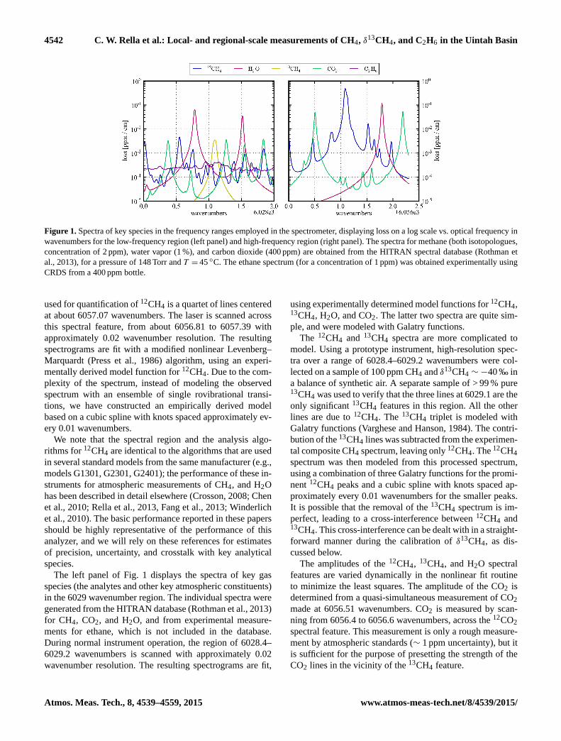
The right panel of Fig. 1 displays the spectra of key gas
species, which includes the five analytical species and other
atmospheric constituents that absorb in the 6057 wavenum-
ber region, generated with the HITRAN database (Rothman
et al., 2013) for CH4, CO2, and H2O. The spectral feature
www.atmos-meas-tech.net/8/4539/2015/ Atmos. Meas. Tech., 8, 4539–4559, 2015
4542 C. W. Rella et al.: Local- and regional-scale measurements of CH4, δ13CH4, and C2H6 in the Uintah Basin
Figure 1. Spectra of key species in the frequency ranges employed in the spectrometer, displaying loss on a log scale vs. optical frequency in
wavenumbers for the low-frequency region (left panel) and high-frequency region (right panel). The spectra for methane (both isotopologues,
concentration of 2 ppm), water vapor (1 %), and carbon dioxide (400 ppm) are obtained from the HITRAN spectral database (Rothman et
al., 2013), for a pressure of 148 Torr and T = 45 ◦C. The ethane spectrum (for a concentration of 1 ppm) was obtained experimentally using
CRDS from a 400 ppm bottle.
used for quantification of 12CH4 is a quartet of lines centered
at about 6057.07 wavenumbers. The laser is scanned across
this spectral feature, from about 6056.81 to 6057.39 with
approximately 0.02 wavenumber resolution. The resulting
spectrograms are fit with a modified nonlinear Levenberg–
Marquardt (Press et al., 1986) algorithm, using an experi-
mentally derived model function for 12CH4. Due to the com-
plexity of the spectrum, instead of modeling the observed
spectrum with an ensemble of single rovibrational transi-
tions, we have constructed an empirically derived model
based on a cubic spline with knots spaced approximately ev-
ery 0.01 wavenumbers.
We note that the spectral region and the analysis algo-
rithms for 12CH4 are identical to the algorithms that are used
in several standard models from the same manufacturer (e.g.,
models G1301, G2301, G2401); the performance of these in-
struments for atmospheric measurements of CH4, and H2O
has been described in detail elsewhere (Crosson, 2008; Chen
et al., 2010; Rella et al., 2013, Fang et al., 2013; Winderlich
et al., 2010). The basic performance reported in these papers
should be highly representative of the performance of this
analyzer, and we will rely on these references for estimates
of precision, uncertainty, and crosstalk with key analytical
species.
The left panel of Fig. 1 displays the spectra of key gas
species (the analytes and other key atmospheric constituents)
in the 6029 wavenumber region. The individual spectra were
generated from the HITRAN database (Rothman et al., 2013)
for CH4, CO2, and H2O, and from experimental measure-
ments for ethane, which is not included in the database.
During normal instrument operation, the region of 6028.4–
6029.2 wavenumbers is scanned with approximately 0.02
wavenumber resolution. The resulting spectrograms are fit,
using experimentally determined model functions for 12CH4,13CH4, H2O, and CO2. The latter two spectra are quite sim-
ple, and were modeled with Galatry functions.
The 12CH4 and 13CH4 spectra are more complicated to
model. Using a prototype instrument, high-resolution spec-
tra over a range of 6028.4–6029.2 wavenumbers were col-
lected on a sample of 100 ppm CH4 and δ13CH4 ∼−40 ‰ in
a balance of synthetic air. A separate sample of > 99 % pure13CH4 was used to verify that the three lines at 6029.1 are the
only significant 13CH4 features in this region. All the other
lines are due to 12CH4. The 13CH4 triplet is modeled with
Galatry functions (Varghese and Hanson, 1984). The contri-
bution of the 13CH4 lines was subtracted from the experimen-
tal composite CH4 spectrum, leaving only 12CH4. The 12CH4
spectrum was then modeled from this processed spectrum,
using a combination of three Galatry functions for the promi-
nent 12CH4 peaks and a cubic spline with knots spaced ap-
proximately every 0.01 wavenumbers for the smaller peaks.
It is possible that the removal of the 13CH4 spectrum is im-
perfect, leading to a cross-interference between 12CH4 and13CH4. This cross-interference can be dealt with in a straight-
forward manner during the calibration of δ13CH4, as dis-
cussed below.
The amplitudes of the 12CH4, 13CH4, and H2O spectral
features are varied dynamically in the nonlinear fit routine
to minimize the least squares. The amplitude of the CO2 is
determined from a quasi-simultaneous measurement of CO2
made at 6056.51 wavenumbers. CO2 is measured by scan-
ning from 6056.4 to 6056.6 wavenumbers, across the 12CO2
spectral feature. This measurement is only a rough measure-
ment by atmospheric standards (∼ 1 ppm uncertainty), but it
is sufficient for the purpose of presetting the strength of the
CO2 lines in the vicinity of the 13CH4 feature.
Atmos. Meas. Tech., 8, 4539–4559, 2015 www.atmos-meas-tech.net/8/4539/2015/
C. W. Rella et al.: Local- and regional-scale measurements of CH4, δ13CH4, and C2H6 in the Uintah Basin 4543
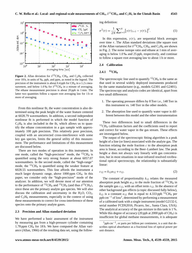
Figure 2. Allan deviation for δ13CH4, CH4, and C2H6 collected
over 18 h, in units of ‰, ppb, and ppm, as noted in the legend. The
precision of the instrument is about 0.4 ppb for CH4 in a 1.2 s mea-
surement, and below 1.0 ‰ for δ13CH4 in a minute of averaging.
The ethane measurement precision is about 20 ppb in 1 min. The
latter two quantities follow a square root averaging law for 1 h or
more of averaging.
From this nonlinear fit, the water concentration is also de-
termined using the peak height of the water feature centered
at 6028.79 wavenumbers. In addition, a second independent
nonlinear fit is performed in which the model function of
C2H6 is also included in the fit, which allows us to quan-
tify the ethane concentration in a gas sample with approx-
imately 100 ppb precision. This relatively poor precision,
coupled with an uncorrected cross-interference with some
key gas species, limits the general utility of this measure-
ment. The performance and limitations of this measurement
are discussed below.
There are two modes of operation in this instrument. In
one mode, called the “high-precision” mode, the 12CH4 is
quantified using the very strong feature at about 6057.07
wavenumbers. In the second mode, called the “high-range”
mode, the 12CH4 is quantified using the weaker feature at
6028.55 wavenumbers. This line affords the instrument a
much larger dynamic range, above 1000 ppm CH4. In this
paper, we consider only the “high-precision” mode of the
analyzer. In addition, we will devote most of our attention
to the performance of 12CH4 and 13CH4 (and thus δ13CH4),
since these are the primary analyte gas species. We will also
discuss the calibration and uncertainty in the H2O, CO2,
and C2H6 measurements, especially in the context of using
these measurements to correct for cross-interference of these
species onto the primary analyte gases.
2.3 Precision and Allan standard deviation
We have performed a basic assessment of the instrument
by measuring gas from a high-pressure cylinder containing
1.78 ppm CH4 for 18 h. We have computed the Allan vari-
ance (Allan, 1966) of the resulting data set, using the follow-
ing definition:
σ 2(τ )=1
2N
∑N
i=1
[y(τ)i+1− y(τ)i
]2. (1)
In this expression, y(τ)i are sequential block averages
over time τ . The Allan standard deviations (the square root
of the Allan variance) for δ13CH4, CH4, and C2H6 are shown
in Fig. 2. The noise isotope ratio and ethane at 1 min of aver-
aging is below 1.0 ‰ and 25 ppb, respectively, and continue
to follow a square root averaging law to about 1 h or more.
2.4 Calibration
2.4.1 12CH4
The spectroscopic line used to quantify 12CH4 is the same as
that used in several widely deployed instruments produced
by the same manufacturer (e.g., models G2301 and G2401).
The spectroscopy and analysis codes are identical, apart from
two small differences:
1. The operating pressure differs by 8 Torr i.e., 148 Torr in
this instrument vs. 140 Torr in the other models.
2. The absorption line used to quantify water vapor is dif-
ferent between this model and the other instrumentation
These two differences lead to small differences in the12CH4 calibration factors and the coefficients used to report
and correct for water vapor in the gas stream. These effects
are investigated below.
The output of the spectroscopic fitting algorithm is a peak
height of a line (or lines) associated with the analyte gas. The
function relating the mole fraction c to the absorption peak
area is linear, according to the Beer–Lambert law. The peak
height α does not always vary linearly with gas concentra-
tion, but in most situations in near-infrared resolved rovibra-
tional optical spectroscopy, the relationship is substantially
linear:
c12 = k12α12+ ε12. (2)
The constant of proportionality k12 relates the measured
absorption peak height α12 to the mole fraction of 12CH4 in
the sample gas c12, with an offset term ε12. In the absence of
other background gas effects (a topic discussed fully below),
k12 is a constant κ12 that is equal to 4.333 ppb 12CH4 per
ppb cm−1 of loss1, determined by performing a measurement
of a calibrated tank with a single instrument (model G2132-I,
serial number FCDS2016, Picarro, Inc., Santa Clara, USA).
The analytical accuracy of the gas mixture in this tank is 1 %.
While this degree of accuracy (20 ppb at 2000 ppb of CH4) is
insufficient for global methane measurements, it is adequate
1ppb cm−1, or parts per billion per centimeter, is a unit that de-
scribes optical absorbance as a fractional loss of optical power per
unit distance.
www.atmos-meas-tech.net/8/4539/2015/ Atmos. Meas. Tech., 8, 4539–4559, 2015
4544 C. W. Rella et al.: Local- and regional-scale measurements of CH4, δ13CH4, and C2H6 in the Uintah Basin
for the purposes of this study in which the typical methane
enhancement was higher than 1000 ppb. For more demanding
applications, the instrument can be calibrated using standard
gas mixtures with lower uncertainty, which also allows one
to determine the offset term ε12 which is typically within a
few parts per billion of zero.
2.4.2 δ13CH4
The 13CH4 concentration is determined from the measured
absorption peak height, using a similar treatment as for12CH4. We begin with the simple linear relationship:
c13 = k13α13+ ε13. (3)
In principle, with careful measurements, we could deter-
mine calibration constants for 13CH4 as was done for 12CH4.
However, we have chosen a strategy of selecting δ13CH4 as
the primary isotopic measurement output, rather than 13CH4,
for the following reasons:
1. It is experimentally more straightforward to generate a
constant δ13CH4 in a varying background gas mixture
than it is to generate a constant 13CH4 mixture.
2. Dilution by other gas species, such as water vapor,
oxygen, or argon, occurs to both species equally (as a
percentage of each species’ dry mole fraction), which
means that δ13CH4 is unaffected by dilution.
3. Spectral line shape effects due to other gas species
are likely to have similar effects on the two methane
species. δ13CH4 is affected only by differences in the
line shape effects between the two species.
4. δ13C is commonly reported on the Vienna Pee Dee
Belemnite scale (Coplen et al., 2006), for which there
are traceable primary standards. In contrast, there are
no independent primary standards for 13CH4; the scale
for 13CH4 is typically defined by a combination of the
δ13CH4 standard and the total CH4 scale.
Throughout this paper, we will consider 12CH4 and
δ13CH4 as the independently calibrated quantities. The in-
dividual concentration 13CH4 will be derived directly from
these two analytical values using the following expression:
δ13CH4[in ‰] ≡ 1000
(rsample
rVPDB
− 1
), (4)
where rsample = c13/c12 and rVPDB = 0.0111802. The value
for rVPDB follows Werner and Brand (2001). Substituting the
simple linear relationships for c12 and c13 (Eqs. 2 and 3) into
this expression, we find
δ13CH4 = 1000
(k13α13+ ε13
(k12α12+ ε12) rVPDB
− 1
). (5)
Equation (5) relates the spectroscopic measurements of
absorption loss at the peak of the two isotopologues (α12 and
α13), the calibration coefficients (k12 and k13), and the cali-
bration offsets (ε12 and ε13) to the determination of δ13CH4.
First, we consider the case of an ideal spectrometer, for
which the calibration coefficients are constants (i.e., k12 =
κ12 and k13 = κ13), and the calibration offsets are zero (i.e.,
ε12 = ε13 = 0). These assumptions lead to the following ex-
pression, as expected:
δ13CH4 = 1000
(κ13α13
κ12α12
)rVPDB
− 1
. (6)
Equation (6) can be used to calibrate the instrument, as it
relates the spectroscopically measurable quantities (i.e., the
peak height ratioα13
α12) to δ13CH4. The factory calibration for
this set of spectroscopic lines was obtained using the follow-
ing method. A single bottle of 100 ppm methane (Air Liq-
uide America Specialty Gases, Plumsteadville, Pennsylva-
nia, USA) was used as a source gas. Several 1 L sampling
bags (Cali-5-Bond™, Calibrated Instruments, Hawthorne,
NY, USA) were filled with the source gas. The bags were
equipped with a silicone septum mounted directly on the bag.
Pure 12CH4 (99.9 atom %, no. 490210, Sigma Aldrich, St.
Louis, MO, USA) was injected through the septum in vary-
ing amounts to each bag to shift the isotope ratio in the sam-
ples. These bags were then measured on an instrument (se-
rial number FCDS002) after diluting 10 : 1 with methane-free
zero air, and then these bags were subsequently sent for anal-
ysis at a commercial laboratory (Isotech, Champaign, Illi-
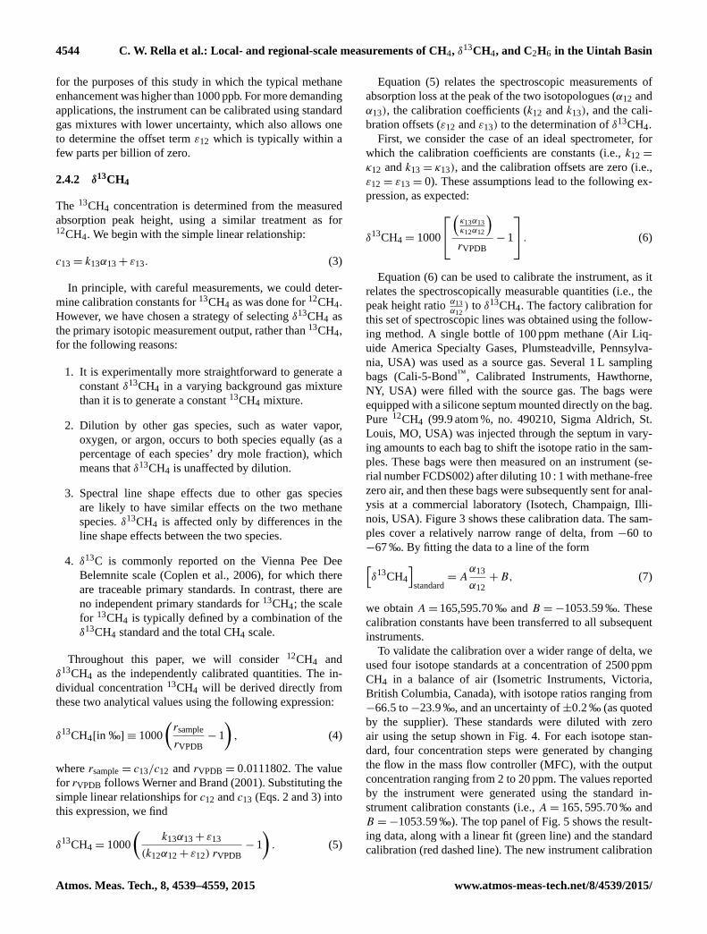
nois, USA). Figure 3 shows these calibration data. The sam-
ples cover a relatively narrow range of delta, from −60 to
−67 ‰. By fitting the data to a line of the form[δ13CH4
]standard
= Aα13
α12
+B, (7)
we obtain A= 165,595.70 ‰ and B =−1053.59 ‰. These
calibration constants have been transferred to all subsequent
instruments.
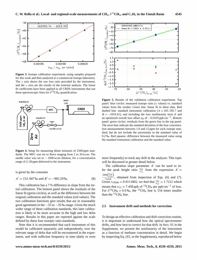
To validate the calibration over a wider range of delta, we
used four isotope standards at a concentration of 2500 ppm
CH4 in a balance of air (Isometric Instruments, Victoria,
British Columbia, Canada), with isotope ratios ranging from
−66.5 to−23.9 ‰, and an uncertainty of±0.2 ‰ (as quoted
by the supplier). These standards were diluted with zero
air using the setup shown in Fig. 4. For each isotope stan-
dard, four concentration steps were generated by changing
the flow in the mass flow controller (MFC), with the output
concentration ranging from 2 to 20 ppm. The values reported
by the instrument were generated using the standard in-
strument calibration constants (i.e., A= 165,595.70 ‰ and
B =−1053.59 ‰). The top panel of Fig. 5 shows the result-
ing data, along with a linear fit (green line) and the standard
calibration (red dashed line). The new instrument calibration
Atmos. Meas. Tech., 8, 4539–4559, 2015 www.atmos-meas-tech.net/8/4539/2015/
C. W. Rella et al.: Local- and regional-scale measurements of CH4, δ13CH4, and C2H6 in the Uintah Basin 4545
Figure 3. Isotope calibration experiment, using samples prepared
for this work and then analyzed at a commercial isotope laboratory.
The x axis shows the raw loss ratio provided by the instrument,
and the y axis are the results of the external analysis. The linear
fit coefficients have been applied to all CRDS instruments that use
these spectroscopic lines for δ13CH4 quantification.
Figure 4. Setup for measuring dilute mixtures of 2500 ppm stan-
dards. The MFC was set to flows ranging from 2 to 20 sccm. The
needle valve was set to ∼ 1000 sccm dilution, for a concentration
range of 2–20 ppm delivered to the instrument.
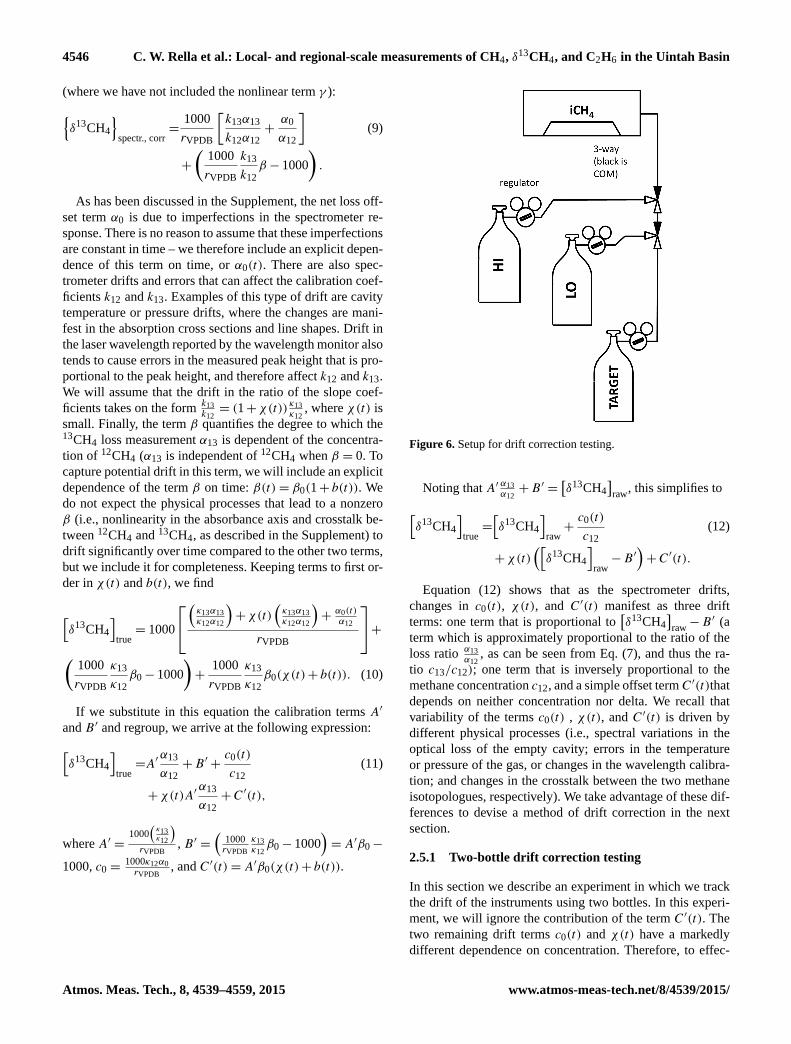
is given by the constants
A′ = 153,947‰ and B ′ =−983.29‰. (8)
This calibration has a 7 % difference in slope from the ini-
tial calibration. The bottom panel shows the residuals of the
linear fit (green circles), as well as the difference between the
original calibration and the standard values (red values). The
two calibration functions give results that are in reasonably
good agreement in the−55 to−35 ‰ range. Given the much
wider range of these calibration standards, this later calibra-
tion is likely to be more accurate in the high and low delta
ranges. Results in this paper are reported against the scale
defined by these four isotopic ratio standards.
Note that it is recommended that each instrument of this
model be calibrated separately and independently, over the
relevant range of delta that will be encountered in the exper-
iment, and with sufficient frequency in time (daily or even
Figure 5. Results of the validation calibration experiment. Top
panel: blue circles: measured isotope ratio (x values) vs. standard
values from the vendor. Green line: linear fit to these data. Red
dashed line: standard instrument calibration (A= 165,595.7 and
B =−1053.61), and including the loss nonlinearity term β and
an optimized overall loss offset α0 of −0.0103 ppb cm−1. Bottom
panel: green circles: residuals from the green line in the top panel.
The error bars indicate the standard deviation of the four concentra-
tion measurements between 1.9 and 15 ppm for each isotope stan-
dard, but do not include the uncertainty in the standard value of
0.2 ‰. Red squares: difference between the measured value using
the standard instrument calibration and the standard value.
more frequently) to track any drift in the analyzer. This topic
will be discussed in greater detail below.
The calibration slope parameter A′ can be used to in-
fer the peak height ratioκ13
κ12from the expression A′ =
1000(κ13κ12
)rVPDB
, obtained from inspection of Eqs. (6) and (7).
Given rVPDB = 0.0111802, we find thatκ13
κ12= 1.7212 which
means that κ13 = 7.458 ppb of 13CH4 per ppb cm−1 of loss.
For δ13CH4 = 0.0 ‰, the 13CH4 line is 154 times smaller
than the 12CH4 line.
2.5 Instrument drift and methods for correction
To design an effective calibration and drift correction routine,
it is important to understand how the optical spectrometer
drifts, and how best to correct for that drift. In Sect. S1 in the
Supplement, we present the nonlinearity of the instrument
as a function of methane concentration in detail. We begin
by inspecting Eq. (S5, in the Supplement), reproduced below
www.atmos-meas-tech.net/8/4539/2015/ Atmos. Meas. Tech., 8, 4539–4559, 2015
4546 C. W. Rella et al.: Local- and regional-scale measurements of CH4, δ13CH4, and C2H6 in the Uintah Basin
(where we have not included the nonlinear term γ ):{δ13CH4
}spectr., corr
=1000
rVPDB
[k13α13
k12α12
+α0
α12
](9)
+
(1000
rVPDB
k13
k12
β − 1000
).
As has been discussed in the Supplement, the net loss off-
set term α0 is due to imperfections in the spectrometer re-
sponse. There is no reason to assume that these imperfections
are constant in time – we therefore include an explicit depen-
dence of this term on time, or α0(t). There are also spec-
trometer drifts and errors that can affect the calibration coef-
ficients k12 and k13. Examples of this type of drift are cavity
temperature or pressure drifts, where the changes are mani-
fest in the absorption cross sections and line shapes. Drift in
the laser wavelength reported by the wavelength monitor also
tends to cause errors in the measured peak height that is pro-
portional to the peak height, and therefore affect k12 and k13.
We will assume that the drift in the ratio of the slope coef-
ficients takes on the formk13
k12= (1+χ(t))
κ13
κ12, where χ(t) is
small. Finally, the term β quantifies the degree to which the13CH4 loss measurement α13 is dependent of the concentra-
tion of 12CH4 (α13 is independent of 12CH4 when β = 0. To
capture potential drift in this term, we will include an explicit
dependence of the term β on time: β(t)= β0(1+ b(t)). We
do not expect the physical processes that lead to a nonzero
β (i.e., nonlinearity in the absorbance axis and crosstalk be-
tween 12CH4 and 13CH4, as described in the Supplement) to
drift significantly over time compared to the other two terms,
but we include it for completeness. Keeping terms to first or-
der in χ(t) and b(t), we find
[δ13CH4
]true= 1000
(κ13α13
κ12α12
)+χ(t)
(κ13α13
κ12α12
)+α0(t)α12
rVPDB
+(
1000
rVPDB
κ13
κ12
β0− 1000
)+
1000
rVPDB
κ13
κ12
β0(χ(t)+ b(t)). (10)
If we substitute in this equation the calibration terms A′
and B ′ and regroup, we arrive at the following expression:[δ13CH4
]true=A′
α13
α12
+B ′+c0(t)
c12
(11)
+χ(t)A′α13
α12
+C′(t),
where A′ =1000
(κ13κ12
)rVPDB
, B ′ =(
1000rVPDB
κ13
κ12β0− 1000
)= A′β0−
1000, c0 =1000κ12α0
rVPDB, and C′(t)= A′β0(χ(t)+ b(t)).
Figure 6. Setup for drift correction testing.
Noting that A′α13
α12+B ′ =
[δ13CH4
]raw
, this simplifies to[δ13CH4
]true=
[δ13CH4
]raw+c0(t)
c12
(12)
+χ(t)([δ13CH4
]raw−B ′
)+C′(t).
Equation (12) shows that as the spectrometer drifts,
changes in c0(t), χ(t), and C′(t) manifest as three drift
terms: one term that is proportional to[δ13CH4
]raw−B ′ (a
term which is approximately proportional to the ratio of the
loss ratioα13
α12, as can be seen from Eq. (7), and thus the ra-
tio c13/c12); one term that is inversely proportional to the
methane concentration c12, and a simple offset termC′(t)that
depends on neither concentration nor delta. We recall that
variability of the terms c0(t) , χ(t), and C′(t) is driven by
different physical processes (i.e., spectral variations in the
optical loss of the empty cavity; errors in the temperature
or pressure of the gas, or changes in the wavelength calibra-
tion; and changes in the crosstalk between the two methane
isotopologues, respectively). We take advantage of these dif-
ferences to devise a method of drift correction in the next
section.
2.5.1 Two-bottle drift correction testing
In this section we describe an experiment in which we track
the drift of the instruments using two bottles. In this experi-
ment, we will ignore the contribution of the term C′(t). The
two remaining drift terms c0(t) and χ(t) have a markedly
different dependence on concentration. Therefore, to effec-
Atmos. Meas. Tech., 8, 4539–4559, 2015 www.atmos-meas-tech.net/8/4539/2015/
C. W. Rella et al.: Local- and regional-scale measurements of CH4, δ13CH4, and C2H6 in the Uintah Basin 4547
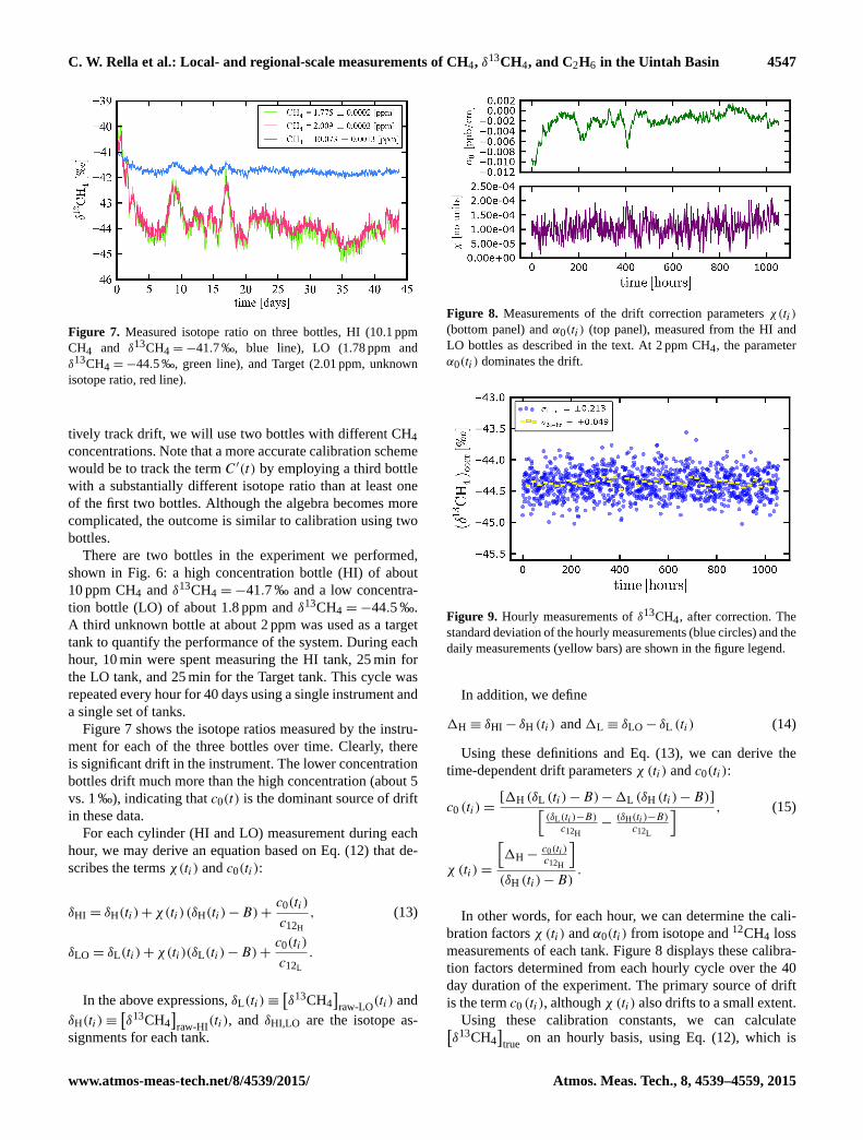
Figure 7. Measured isotope ratio on three bottles, HI (10.1 ppm
CH4 and δ13CH4 =−41.7 ‰, blue line), LO (1.78 ppm and
δ13CH4 =−44.5 ‰, green line), and Target (2.01 ppm, unknown
isotope ratio, red line).
tively track drift, we will use two bottles with different CH4
concentrations. Note that a more accurate calibration scheme
would be to track the term C′(t) by employing a third bottle
with a substantially different isotope ratio than at least one
of the first two bottles. Although the algebra becomes more
complicated, the outcome is similar to calibration using two
bottles.
There are two bottles in the experiment we performed,
shown in Fig. 6: a high concentration bottle (HI) of about
10 ppm CH4 and δ13CH4 =−41.7 ‰ and a low concentra-
tion bottle (LO) of about 1.8 ppm and δ13CH4 =−44.5 ‰.
A third unknown bottle at about 2 ppm was used as a target
tank to quantify the performance of the system. During each
hour, 10 min were spent measuring the HI tank, 25 min for
the LO tank, and 25 min for the Target tank. This cycle was
repeated every hour for 40 days using a single instrument and
a single set of tanks.
Figure 7 shows the isotope ratios measured by the instru-
ment for each of the three bottles over time. Clearly, there
is significant drift in the instrument. The lower concentration
bottles drift much more than the high concentration (about 5
vs. 1 ‰), indicating that c0(t) is the dominant source of drift
in these data.
For each cylinder (HI and LO) measurement during each
hour, we may derive an equation based on Eq. (12) that de-
scribes the terms χ(ti) and c0(ti):
δHI = δH(ti)+χ(ti)(δH(ti)−B)+c0(ti)
c12H
, (13)
δLO = δL(ti)+χ(ti)(δL(ti)−B)+c0(ti)
c12L
.
In the above expressions, δL(ti)≡[δ13CH4
]raw-LO
(ti) and
δH(ti)≡[δ13CH4
]raw-HI
(ti), and δHI,LO are the isotope as-
signments for each tank.
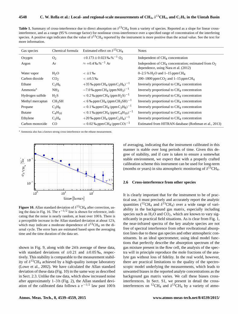
Figure 8. Measurements of the drift correction parameters χ(ti)
(bottom panel) and α0(ti) (top panel), measured from the HI and
LO bottles as described in the text. At 2 ppm CH4, the parameter
α0(ti) dominates the drift.
Figure 9. Hourly measurements of δ13CH4, after correction. The
standard deviation of the hourly measurements (blue circles) and the
daily measurements (yellow bars) are shown in the figure legend.
In addition, we define
1H ≡ δHI− δH (ti) and 1L ≡ δLO− δL (ti) (14)
Using these definitions and Eq. (13), we can derive the
time-dependent drift parameters χ (ti) and c0(ti):
c0 (ti)=[1H (δL (ti)−B)−1L (δH (ti)−B)][
(δL(ti )−B)c12H
−(δH(ti )−B)
c12L
] , (15)
χ (ti)=
[1H−
c0(ti )c12H
](δH (ti)−B)
.
In other words, for each hour, we can determine the cali-
bration factors χ (ti) and α0(ti) from isotope and 12CH4 loss
measurements of each tank. Figure 8 displays these calibra-
tion factors determined from each hourly cycle over the 40
day duration of the experiment. The primary source of drift
is the term c0 (ti), although χ (ti) also drifts to a small extent.
Using these calibration constants, we can calculate[δ13CH4
]true
on an hourly basis, using Eq. (12), which is
www.atmos-meas-tech.net/8/4539/2015/ Atmos. Meas. Tech., 8, 4539–4559, 2015
4548 C. W. Rella et al.: Local- and regional-scale measurements of CH4, δ13CH4, and C2H6 in the Uintah Basin
Table 1. Summary of cross-interference due to direct absorption on δ13CH4 from a variety of species. Reported as a slope for linear cross-
interference, and as a range (95 % coverage factor) for nonlinear cross-interference over a specified range of concentration of the interfering
species. A positive sign indicates that the value of δ13CH4 reported by the instrument is more positive than the actual value. See the text for
more information.
Gas species Chemical formula Estimated effect on δ13CH4 Notes
Oxygen O2 +0.173± 0.023 ‰%−1 O2 Independent of CH4 concentration
Argon Ar ≈+0.4 ‰%−1 Ar Independent of CH4 concentration; estimated from O2
dependence, using Nara et al. (2012)
Water vapor H2O <±1 ‰ 0–2.5 % H2O and 1–15 ppmCH4
Carbon dioxide CO2 <±0.5 ‰ 200–1800 ppmCO2 and 1–15 ppmCH4
Ethane C2H6 +35 ‰ppmCH4 (ppmC2H6)−1 Inversely proportional to CH4 concentration
Ammonia∗ NH3 −7.0 ‰ppmCH4 (ppmNH3)−1 Inversely proportional to CH4 concentration
Hydrogen sulfide H2S < 0.2 ‰ppmCH4 (ppmH2S)−1 Inversely proportional to CH4 concentration
Methyl mercaptan CH3SH < 6 ‰ppmCH4 (ppmCH3SH)−1 Inversely proportional to CH4 concentration
Propane C3H8 < 0.1 ‰ppmCH4 (ppmC3H8)−1 Inversely proportional to CH4 concentration
Butane C4H10 < 0.1 ‰ppmCH4 (ppmC4H10)−1 Inversely proportional to CH4 concentration
Ethylene C2H4 +20 ‰ppmCH4 (ppmC2H4)−1 Inversely proportional to CH4 concentration
Carbon monoxide CO < 0.02 ‰ppmCH4 (ppmCO)−1 Estimated from HITRAN database (Rothman et al., 2013)
∗ Ammonia also has a known strong cross-interference on the ethane measurement.
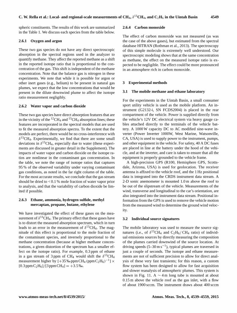
Figure 10. Allan standard deviation of δ13CH4 after correction, us-
ing the data in Fig. 16. The τ−1/2 line is shown for reference, indi-
cating that the noise is nearly random, at least over 100 h. There is
a perceptible increase in the Allan standard deviation at about 12 h,
which may indicate a moderate dependence of δ13CH4 on the di-
urnal cycle. The error bars are estimated based upon the averaging
time and the time duration of the data set.
shown in Fig. 9, along with the 24 h average of these data,
with standard deviations of ±0.21 and ±0.05 ‰, respec-
tively. This stability is comparable to the measurement stabil-
ity of δ13CH4 achieved by a high-quality isotope laboratory
(Lowe et al., 2002). We have calculated the Allan standard
deviation of these data (Fig. 10) in the same way as described
in Sect. 2.3. Unlike the raw data, which show increased noise
after approximately 1–3 h (Fig. 2), the Allan standard devi-
ation of the calibrated data follows a τ−1/2 law past 100 h
of averaging, indicating that the instrument calibrated in this
manner is stable over long periods of time. Given this de-
gree of stability, and if care is taken to ensure a somewhat
stable environment, we expect that with a properly crafted
calibration scheme this instrument can be used for long-term
(months or years) in situ atmospheric monitoring of δ13CH4.
2.6 Cross-interference from other species
It is clearly important that for the instrument to be of prac-
tical use, it must precisely and accurately report the analytic
quantities (12CH4 and δ13CH4) over a wide range of vari-
ability in the background gas matrix, especially including
species such as H2O and CO2, which are known to vary sig-
nificantly in practical field situations. As is clear from Fig. 1,
the near-infrared spectra of the key analyte species are not
free of spectral interference from other rovibrational absorp-
tion lines due to these gas species and other atmospheric con-
stituents. In an ideal spectrometer, using ideal model func-
tions that perfectly describe the absorption spectrum of the
gas mixture present in the flow cell, the analysis of the spec-
tra will in principle reproduce the mole fractions of the ana-
lyte gas without loss of fidelity. In the real world, however,
there are practical limitations to the quality of the spectro-
scopic model underlying the measurements, which leads to
unwanted biases in the reported analyte concentrations as the
background gas matrix varies. We call these biases cross-
interferences. In Sect. S1, we present in detail the cross-
interferences on 12CH4 and δ13CH4 by a variety of atmo-
Atmos. Meas. Tech., 8, 4539–4559, 2015 www.atmos-meas-tech.net/8/4539/2015/
C. W. Rella et al.: Local- and regional-scale measurements of CH4, δ13CH4, and C2H6 in the Uintah Basin 4549
spheric constituents. The results of this work are summarized
in the Table 1. We discuss each species from the table below.
2.6.1 Oxygen and argon
These two gas species do not have any direct spectroscopic
absorption in the spectral regions used in the analyzer to
quantify methane. They affect the reported methane as a shift
in the reported isotope ratio that is proportional to the con-
centration of the gas. This shift is independent of the methane
concentration. Note that the balance gas is nitrogen in these
experiments. We note that while it is possible for argon or
other inert gases (e.g., helium) to be present in natural gas
plumes, we expect that the low concentrations that would be
present in the dilute downwind plume to affect the isotope
ratio measurement negligibly.
2.6.2 Water vapor and carbon dioxide
These two gas species have direct absorption features that are
in the vicinity of the 12CH4 and 13CH4 absorption lines; these
features are incorporated in the spectral models that are used
to fit the measured absorption spectra. To the extent that the
models are perfect, there would be no cross-interference with
δ13CH4. Experimentally, we find that there are some small
deviations in δ13CH4, especially due to water (these experi-
ments are discussed in greater detail in the Supplement). The
impacts of water vapor and carbon dioxide on the isotope ra-
tios are nonlinear in the contaminant gas concentration. In
the table, we note the range of isotope ratios that captures
95 % of the observed variability under varying contaminant
gas conditions, as noted in the far right column of the table.
For the most accurate results, we conclude that the gas stream
should be dried to < 0.1 % mole fraction of water vapor prior
to analysis, and that the variability of carbon dioxide be lim-
ited if possible.
2.6.3 Ethane, ammonia, hydrogen sulfide, methyl
mercaptan, propane, butane, ethylene
We have investigated the effect of these gases on the mea-
surement of δ13CH4. The primary effect that these gases have
is to distort the measured absorption spectrum, which in turn
leads to an error in the measurement of δ13CH4. The mag-
nitude of this effect is proportional to the mole fraction of
the contaminant species, and inversely proportional to the
methane concentration (because at higher methane concen-
trations, a given distortion of the spectrum has a smaller ef-
fect on the isotope ratio). For example, 0.3 ppm of ethane
in a gas stream of 3 ppm of CH4 would shift the δ13CH4
measurement higher by [+35‰ppmCH4 (ppmC2H6)−1]×
[0.3ppmC2H6]/[3 ppmCH4] = +3.5‰.
2.6.4 Carbon monoxide
The effect of carbon monoxide was not measured (as was
the case of the above gases), but estimated from the spectral
database HITRAN (Rothman et al., 2013). The spectroscopy
of this simple molecule is extremely well understood. Our
spectroscopic modeling shows that at the same concentration
as methane, the effect on the measured isotope ratio is ex-
pected to be negligible. The effect could be more pronounced
in an atmosphere rich in carbon monoxide.
3 Experimental methods
3.1 The mobile methane and ethane laboratory
For the experiments in the Uintah Basin, a small consumer
sport utility vehicle is used as the mobile platform. An in-
strument (G2132-i, SN FCDS2004) is placed in the rear
compartment of the vehicle. Power is supplied directly from
the vehicle’s 12V DC electrical system via heavy gauge ca-
bles attached directly to the terminals of the vehicle bat-
tery. A 1000 W capacity DC to AC modified sine-wave in-
verter (Power Inverter 1000W, West Marine, Watsonville,
CA, USA) is used to supply power to the instrument, pumps,
and other equipment in the vehicle. For safety, 40 A DC fuses
are placed in line at the battery under the hood of the vehi-
cle, and at the inverter, and care is taken to ensure that all the
equipment is properly grounded to the vehicle frame.
A high-precision GPS (R100, Hemisphere GPS, Scotts-
dale, Arizona, USA) is used for geolocation. The receiver
antenna is affixed to the vehicle roof, and the 1 Hz positional
data is integrated into the CRDS instrument data stream. A
2-D sonic anemometer is mounted 1.0 m above the roof to
be out of the slipstream of the vehicle. Measurements of the
wind, transverse and longitudinal to the car’s orientation, are
also integrated into the instrument data stream. Positional in-
formation from the GPS is used to remove the vehicle motion
from the measured wind to determine the ground wind veloc-
ity.
3.2 Individual source signatures
The mobile laboratory was used to measure the source sig-
natures (i.e., of δ13CH4 and C2H6/CH4 ratio) of individ-
ual emissions sources by directly measuring the composition
of the plumes carried downwind of the source location. At
driving speeds (5–30 m s−1), typical plumes are traversed in
just a couple of seconds. The isotope and ethane measure-
ments are not of sufficient precision to allow for direct anal-
ysis of these very fast transients; for this reason, a custom
flow system has been designed to allow for fast acquisition
and slower reanalysis of atmospheric plumes. This system is
shown in Fig. 11. A ∼ 4 m long tube is mounted at about
0.15 m above the vehicle roof as the gas inlet, with a flow
of about 1900 sccm. The instrument draws about 400 sccm
www.atmos-meas-tech.net/8/4539/2015/ Atmos. Meas. Tech., 8, 4539–4559, 2015
4550 C. W. Rella et al.: Local- and regional-scale measurements of CH4, δ13CH4, and C2H6 in the Uintah Basin
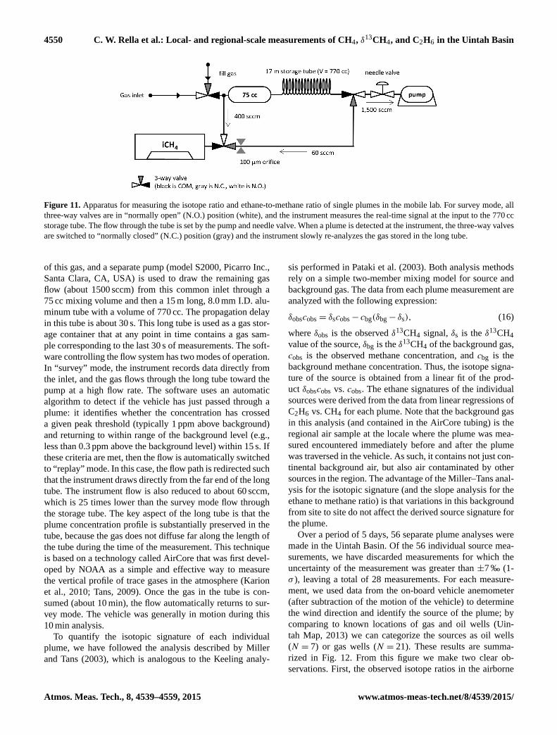
Figure 11. Apparatus for measuring the isotope ratio and ethane-to-methane ratio of single plumes in the mobile lab. For survey mode, all
three-way valves are in “normally open” (N.O.) position (white), and the instrument measures the real-time signal at the input to the 770 cc
storage tube. The flow through the tube is set by the pump and needle valve. When a plume is detected at the instrument, the three-way valves
are switched to “normally closed” (N.C.) position (gray) and the instrument slowly re-analyzes the gas stored in the long tube.
of this gas, and a separate pump (model S2000, Picarro Inc.,
Santa Clara, CA, USA) is used to draw the remaining gas
flow (about 1500 sccm) from this common inlet through a
75 cc mixing volume and then a 15 m long, 8.0 mm I.D. alu-
minum tube with a volume of 770 cc. The propagation delay
in this tube is about 30 s. This long tube is used as a gas stor-
age container that at any point in time contains a gas sam-
ple corresponding to the last 30 s of measurements. The soft-
ware controlling the flow system has two modes of operation.
In “survey” mode, the instrument records data directly from
the inlet, and the gas flows through the long tube toward the
pump at a high flow rate. The software uses an automatic
algorithm to detect if the vehicle has just passed through a
plume: it identifies whether the concentration has crossed
a given peak threshold (typically 1 ppm above background)
and returning to within range of the background level (e.g.,
less than 0.3 ppm above the background level) within 15 s. If
these criteria are met, then the flow is automatically switched
to “replay” mode. In this case, the flow path is redirected such
that the instrument draws directly from the far end of the long
tube. The instrument flow is also reduced to about 60 sccm,
which is 25 times lower than the survey mode flow through
the storage tube. The key aspect of the long tube is that the
plume concentration profile is substantially preserved in the
tube, because the gas does not diffuse far along the length of
the tube during the time of the measurement. This technique
is based on a technology called AirCore that was first devel-
oped by NOAA as a simple and effective way to measure
the vertical profile of trace gases in the atmosphere (Karion
et al., 2010; Tans, 2009). Once the gas in the tube is con-
sumed (about 10 min), the flow automatically returns to sur-
vey mode. The vehicle was generally in motion during this
10 min analysis.
To quantify the isotopic signature of each individual
plume, we have followed the analysis described by Miller
and Tans (2003), which is analogous to the Keeling analy-
sis performed in Pataki et al. (2003). Both analysis methods
rely on a simple two-member mixing model for source and
background gas. The data from each plume measurement are
analyzed with the following expression:
δobscobs = δscobs− cbg(δbg− δs), (16)
where δobs is the observed δ13CH4 signal, δs is the δ13CH4
value of the source, δbg is the δ13CH4 of the background gas,
cobs is the observed methane concentration, and cbg is the
background methane concentration. Thus, the isotope signa-
ture of the source is obtained from a linear fit of the prod-
uct δobscobs vs. cobs. The ethane signatures of the individual
sources were derived from the data from linear regressions of
C2H6 vs. CH4 for each plume. Note that the background gas
in this analysis (and contained in the AirCore tubing) is the
regional air sample at the locale where the plume was mea-
sured encountered immediately before and after the plume
was traversed in the vehicle. As such, it contains not just con-
tinental background air, but also air contaminated by other
sources in the region. The advantage of the Miller–Tans anal-
ysis for the isotopic signature (and the slope analysis for the
ethane to methane ratio) is that variations in this background
from site to site do not affect the derived source signature for
the plume.
Over a period of 5 days, 56 separate plume analyses were
made in the Uintah Basin. Of the 56 individual source mea-
surements, we have discarded measurements for which the
uncertainty of the measurement was greater than ±7 ‰ (1-
σ ), leaving a total of 28 measurements. For each measure-
ment, we used data from the on-board vehicle anemometer
(after subtraction of the motion of the vehicle) to determine
the wind direction and identify the source of the plume; by
comparing to known locations of gas and oil wells (Uin-
tah Map, 2013) we can categorize the sources as oil wells
(N = 7) or gas wells (N = 21). These results are summa-
rized in Fig. 12. From this figure we make two clear ob-
servations. First, the observed isotope ratios in the airborne
Atmos. Meas. Tech., 8, 4539–4559, 2015 www.atmos-meas-tech.net/8/4539/2015/
C. W. Rella et al.: Local- and regional-scale measurements of CH4, δ13CH4, and C2H6 in the Uintah Basin 4551
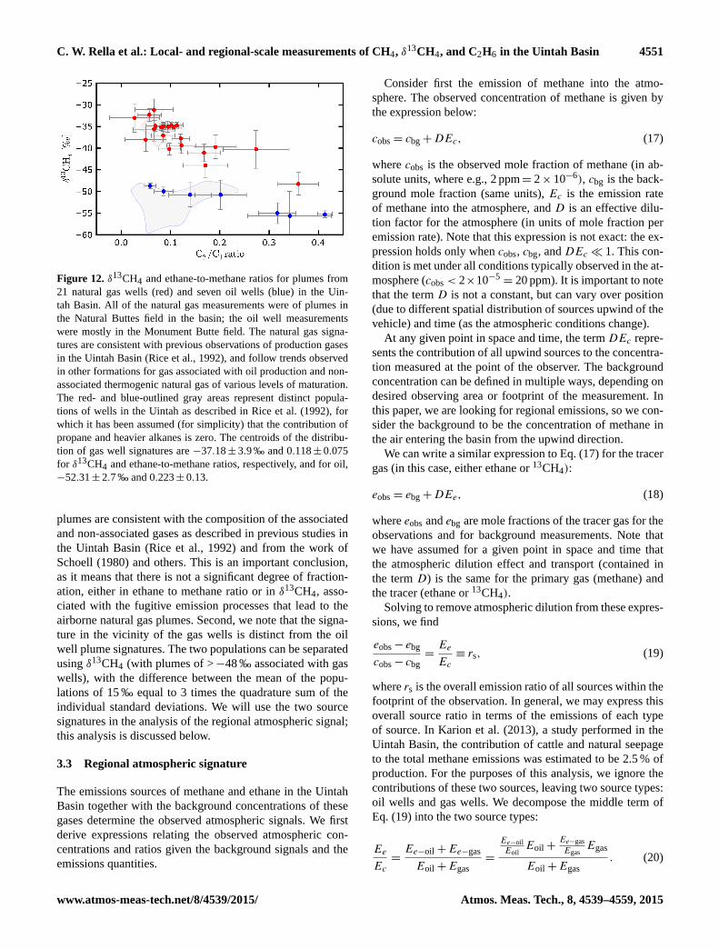
Figure 12. δ13CH4 and ethane-to-methane ratios for plumes from
21 natural gas wells (red) and seven oil wells (blue) in the Uin-
tah Basin. All of the natural gas measurements were of plumes in
the Natural Buttes field in the basin; the oil well measurements
were mostly in the Monument Butte field. The natural gas signa-
tures are consistent with previous observations of production gases
in the Uintah Basin (Rice et al., 1992), and follow trends observed
in other formations for gas associated with oil production and non-
associated thermogenic natural gas of various levels of maturation.
The red- and blue-outlined gray areas represent distinct popula-
tions of wells in the Uintah as described in Rice et al. (1992), for
which it has been assumed (for simplicity) that the contribution of
propane and heavier alkanes is zero. The centroids of the distribu-
tion of gas well signatures are −37.18± 3.9 ‰ and 0.118± 0.075
for δ13CH4 and ethane-to-methane ratios, respectively, and for oil,
−52.31± 2.7 ‰ and 0.223± 0.13.
plumes are consistent with the composition of the associated
and non-associated gases as described in previous studies in
the Uintah Basin (Rice et al., 1992) and from the work of
Schoell (1980) and others. This is an important conclusion,
as it means that there is not a significant degree of fraction-
ation, either in ethane to methane ratio or in δ13CH4, asso-
ciated with the fugitive emission processes that lead to the
airborne natural gas plumes. Second, we note that the signa-
ture in the vicinity of the gas wells is distinct from the oil
well plume signatures. The two populations can be separated
using δ13CH4 (with plumes of >−48 ‰ associated with gas
wells), with the difference between the mean of the popu-
lations of 15 ‰ equal to 3 times the quadrature sum of the
individual standard deviations. We will use the two source
signatures in the analysis of the regional atmospheric signal;
this analysis is discussed below.
3.3 Regional atmospheric signature
The emissions sources of methane and ethane in the Uintah
Basin together with the background concentrations of these
gases determine the observed atmospheric signals. We first
derive expressions relating the observed atmospheric con-
centrations and ratios given the background signals and the
emissions quantities.
Consider first the emission of methane into the atmo-
sphere. The observed concentration of methane is given by
the expression below:
cobs = cbg+DEc, (17)
where cobs is the observed mole fraction of methane (in ab-
solute units, where e.g., 2 ppm= 2× 10⁻⁶), cbg is the back-
ground mole fraction (same units), Ec is the emission rate
of methane into the atmosphere, and D is an effective dilu-
tion factor for the atmosphere (in units of mole fraction per
emission rate). Note that this expression is not exact: the ex-
pression holds only when cobs, cbg, and DEc� 1. This con-
dition is met under all conditions typically observed in the at-
mosphere (cobs < 2×10−5= 20 ppm). It is important to note
that the term D is not a constant, but can vary over position
(due to different spatial distribution of sources upwind of the
vehicle) and time (as the atmospheric conditions change).
At any given point in space and time, the term DEc repre-
sents the contribution of all upwind sources to the concentra-
tion measured at the point of the observer. The background
concentration can be defined in multiple ways, depending on
desired observing area or footprint of the measurement. In
this paper, we are looking for regional emissions, so we con-
sider the background to be the concentration of methane in
the air entering the basin from the upwind direction.
We can write a similar expression to Eq. (17) for the tracer
gas (in this case, either ethane or 13CH4):
eobs = ebg+DEe, (18)
where eobs and ebg are mole fractions of the tracer gas for the
observations and for background measurements. Note that
we have assumed for a given point in space and time that
the atmospheric dilution effect and transport (contained in
the term D) is the same for the primary gas (methane) and
the tracer (ethane or 13CH4).
Solving to remove atmospheric dilution from these expres-
sions, we find
eobs− ebg
cobs− cbg
=Ee
Ec≡ rs, (19)
where rs is the overall emission ratio of all sources within the
footprint of the observation. In general, we may express this
overall source ratio in terms of the emissions of each type
of source. In Karion et al. (2013), a study performed in the
Uintah Basin, the contribution of cattle and natural seepage
to the total methane emissions was estimated to be 2.5 % of
production. For the purposes of this analysis, we ignore the
contributions of these two sources, leaving two source types:
oil wells and gas wells. We decompose the middle term of
Eq. (19) into the two source types:
Ee
Ec=Ee−oil+Ee−gas
Eoil+Egas
=
Ee−oil
EoilEoil+
Ee−gas
EgasEgas
Eoil+Egas
. (20)
www.atmos-meas-tech.net/8/4539/2015/ Atmos. Meas. Tech., 8, 4539–4559, 2015

4552 C. W. Rella et al.: Local- and regional-scale measurements of CH4, δ13CH4, and C2H6 in the Uintah Basin
Figure 13. Apparatus for making regional isotope and ethane ratio measurements. The top schematic shows the mobile sampling system.
The flow through the long storage tube is set by the pump and needle valve. The two manual valves (V1 and V2) are in the open position
during the measurements, and closed when the survey is complete. An optional flow meter can be inserted in the line upstream of the storage
tube to verify the actual flow into the instrument. An instrument in the vehicle measures the local ambient concentration on a separate inlet.
The storage tube is transported to the laboratory (lower schematic), where the gas stored in the long tube is reanalyzed slowly (with the flow
reversed, so the last gas in is the first out). The reanalysis is periodically interrupted to run one or more calibration standard. A gas drying
system can be introduced downstream of the storage tube in the laboratory to reduce the possible effect of water vapor on the measurements,
but this was not done in the results reported here. A fill gas other than ambient air can be used to denote the end of the sample.
In this expression, Eoil and Egas are the emission rates of
methane from each source type, oil wells and gas wells; sim-
ilarly, Ee−oil and Ee−gas are the tracer emissions from each
source type. Defining roil =Ee−oil
Eoiland rgas =
Ee−gas
Egas, we find
rs =roilEoil+ rgasEgas
Eoil+Egas
. (21)
Using Eq. (21), if we can measure rs (the overall ratio of
the tracer to methane observed in the atmosphere), and given
the source signatures of oil and gas sources roil and rgas ob-
served in Fig. 12, we can determine the relative fraction of
the emissions of oil and gas, without measuring the emission
rates directly.
How can we determine the source emission ratio rs? By
regrouping terms in Eq. (19), and by defining robs = eobs/cobs
and rbg = ebg/cbg, we arrive at the following expression:
eobs = rscobs+(rbg− rs
)cbg. (22)
Note that the source emission ratio rs is obtained from
the slope of a plot of eobs vs. cobs. This equation is con-
structed similarly to the Miller–Tans method for isotope
analysis (Miller and Tans, 2003). In fact, this equation re-
duces to the Miller–Tans equation via algebraic manipula-
tion to convert the ratios rs, robs, and rbg to delta notation via
δ = 1000(
rrVPDB
− 1)
:
δobscobs = δscobs+(δbg− δs
)cbg. (23)
These expressions can be used to quantify the source sig-
natures (rs for ethane and {δ13CH4}s) given the observations
and the background values.
To quantify the emission rates of oil wells relative to gas
wells, we need a method for collecting a representative sam-
ple of the air in the Uintah Basin. We have designed a system
that samples gas over long periods of time from the mobile
lab. This gas sample is analyzed in a stationary laboratory,
where careful calibration and longer measurement times can
be brought to bear to improve the precision and accuracy of
the measurements of δ13CH4 and ethane. The sampling sys-
tem is based on the AirCore concept, but with a much larger
volume. The system is shown in Fig. 13. The top schematic
shows the sampling system in the vehicle. Real-time mea-
surements of the CH4 concentration are also made during the
drive, along with GPS coordinates and local wind speed and
direction. We estimate that by using this larger AirCore we
have improved the precision of the regional air measurement
by about a factor of 3 relative to the in-vehicle measurement,
without the need to carry a compressed air cylinder in the
vehicle.
Atmos. Meas. Tech., 8, 4539–4559, 2015 www.atmos-meas-tech.net/8/4539/2015/
C. W. Rella et al.: Local- and regional-scale measurements of CH4, δ13CH4, and C2H6 in the Uintah Basin 4553
To ensure that the gas sampled in the storage tube is rep-
resentative of the regional air, it is important to have a good
understanding of the inlet flow of the system. Under constant
pressure conditions at the inlet of the system, the flow at the
inlet fin is equal to the flow at the exit of the long storage tube
fout. However, the inlet pressure is not constant while in mo-
tion, due to altitude changes and dynamic pressure changes
due to the Bernoulli Effect. These pressure changes will lead
to flow changes at the inlet of the system, leading to uneven
sampling of the regional air. We have constructed a complete
air flow model that we have demonstrated matches observa-
tions. This model and associated experimental validation is
described in the Supplement.
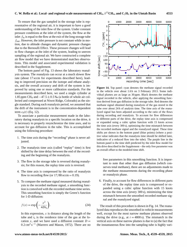
The bottom panel of Fig. 13 shows the laboratory reanal-
ysis system. The reanalysis can occur at a much slower flow
rate (about 17 sccm for experiments described here), lead-
ing to improved precision on the isotope and ethane analy-
sis, and the overall accuracy and drift of the system is im-
proved by using one or more calibration standards. For the
measurements described here, we used a single cylinder at
1.85 ppm CH4 and −47.5± 0.5 ‰ (a bottle of whole air col-
lected and compressed at Niwot Ridge, Colorado) as the sin-
gle standard. During each reanalysis period, we assumed that
the drift of the instrument is in the concentration-dependent
term c0(t) (Eq. 12).
To associate a particular measurement made in the labo-
ratory during reanalysis to a specific location on the drive, it
is necessary to properly resynchronize the time axes, and to
account for gas diffusion in the tube. This is accomplished
using the following procedure:
1. The time axis during the “recording” phase is never ad-
justed.
2. The reanalysis time axis (called “replay” time) is first
shifted by the time delay between the end of the record-
ing and the beginning of the reanalysis.
3. The flow in the storage tube is reversed during reanaly-
sis; for this reason, the replay time axis is reversed.
4. The time axis is compressed by the ratio of reanalysis
flow to recording flow (or 17/88 sccm= 0.19).
5. To compare the methane signal measured during reanal-
ysis to the recorded methane signal, a smoothing func-
tion is convolved with the recorded methane time series.
This smoothing function is simply the Green’s function
for 1-D diffusion:
f (x)= exp
(−x2
4Dts
). (24)
In this expression, x is distance along the length of the
tube and ts is the residence time of the gas at the lo-
cation x, and we have used a diffusion constant D =
0.2 cm2 s−1 (Marrero and Mason, 1972). There are no
Figure 14. Top panel: cyan denotes the methane signal recorded
in the vehicle over about 1.6 h on 3 February 2013. Some indi-
vidual plumes are as large as 30 ppm. Black denotes the methane
signal recorded in the vehicle, after applying the smoothing func-
tion derived from gas diffusion in the storage tube. Red denotes the
methane signal obtained during reanalysis of the gas stored in the
tube over about 24 h of analysis time. The time axis of the reana-
lyzed signal has been adjusted according to the ratio of the flows
during recording and reanalysis. To account for flow differences
in different parts of the drive, the replay time axis is compressed
or expanded using a cubic spline function with 15 knots across
the time axis (every 300 s), optimizing the time mismatch between
the recorded methane signal and the reanalyzed signal. These time
shifts are shown in the bottom panel (blue points) (where a posi-
tive value indicates that the reanalysis time should be shifted later,
indicative of a reduced flow into the tube). The purple line in the
bottom panel is the time shift predicted by the inlet flow model for
this drive described in the Supplement – the only free parameter was
an overall offset to the modeled time shift.
free parameters in this smoothing function. It is impor-
tant to note that other than gas diffusion (which con-
serves total methane), there are no adjustments made to
the methane measurements during the recording phase
or reanalysis phase.
6. Finally, to account for flow differences in different parts
of the drive, the replay time axis is compressed or ex-
panded using a cubic spline function with 15 knots
across the time axis (every 300 s), minimizing the time
mismatch between the smoothed recorded methane sig-
nal and the reanalyzed signal.
The result of this procedure is shown in Fig. 14. The reana-
lyzed data reproduces the smoothed in-vehicle measurements
well, except for the most narrow methane plumes observed
during the drive (e.g., at t = 4800 s). The mismatch in the
vertical axis on these narrow plumes is due to (a) the fact that
the instantaneous flow into the sampling tube is highly vari-
www.atmos-meas-tech.net/8/4539/2015/ Atmos. Meas. Tech., 8, 4539–4559, 2015
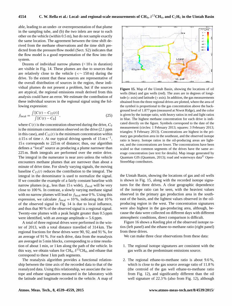
4554 C. W. Rella et al.: Local- and regional-scale measurements of CH4, δ13CH4, and C2H6 in the Uintah Basin
able, leading to an under- or overrepresentation of that plume
in the sampling tube, and (b) the two inlets are near to each
other on the vehicle (within 0.5 m), but do not sample exactly
the same location. The agreement between the time shift de-
rived from the methane observations and the time shift pre-
dicted from the pressure/flow model (Sect. S2) indicates that
the flow model is a good representation of the flow into the
system.
Dozens of individual narrow plumes (< 10 s in duration)
are visible in Fig. 14. These plumes are due to sources that
are relatively close to the vehicle (<∼ 150 m) during the
drive. To the extent that these sources are representative of
the overall distribution of sources in the region, these indi-
vidual plumes do not present a problem, but if the sources
are atypical, the regional emissions result derived from this
analysis could have an error. We estimate the contribution of
these individual sources in the regional signal using the fol-
lowing expression:
flocal =
∫[C(t)−C15(t)]∫
[C(t)−C0], (25)
whereC(t) is the concentration observed during the drive,C0
is the minimum concentration observed on the drive (2.1 ppm
in this case), andC15(t) is the minimum concentration within
±15 s of time t . At our typical driving speeds of 15 m s−1,
15 s corresponds to 225 m of distance; thus, our algorithm
defines a “local” source as producing a plume narrower than
225 m. Both integrals are performed over the entire drive.
The integral in the numerator is near zero unless the vehicle
encounters methane plumes that are narrower than about a
minute of drive time. For slowly varying signals, the moving
baseline C15(t) reduces the contribution to the integral. The
integral in the denominator is used to normalize the signal.
If we consider the example of a fairly constant baseline with
narrow plumes (e.g., less than 15 s wide), flocal will be very
close to 100 %. In contrast, a slowly varying methane signal
with no narrow plumes will lead to flocal near 0 %. Using this
expression, we calculate flocal = 10 %, indicating that 10 %
of the observed signal in Fig. 14 is due to local influence,
and thus that 90 % of the observed signal is a regional signal.
Twenty-one plumes with a peak height greater than 0.5 ppm
were identified, with an average amplitude= 5.6 ppm.
A total of three regional drives were performed in the win-
ter of 2013, with a total distance travelled of 314 km. The
regional fractions for these drives were 90, 92, and 91 %, for
an average of 91 %. For each drive, data from the reanalysis
are averaged in 5 min blocks, corresponding to a time resolu-
tion of about 1 min, or 1 km along the path of the vehicle. In
this way, we obtain values for CH4, δ13CH4, and ethane that
correspond to these 1 km path segments.
The reanalysis algorithm provides a functional relation-
ship between the time axis of the recorded data to that of the
reanalyzed data. Using this relationship, we associate the iso-
tope and ethane signatures measured in the laboratory with
the latitude and longitude recorded in the vehicle. A map of
Figure 15. Map of the Uintah Basin, showing the locations of oil
wells (blue) and gas wells (red). The axes are in degrees of longi-
tude (x axis) and latitude (y axis). In addition, the gas measurements
obtained from the three regional drives are plotted, where the area of
the symbol is proportional to the gas concentration above the back-
ground level of 1.877 ppm (measured at Niwot Ridge), and the color
is given by the isotope ratio, with heavy ratios in red and light ratios
in blue. The highest methane concentration for each drive is indi-
cated directly on the figure. Symbols correspond to the date of the
measurement (circles: 1 February 2013; squares: 3 February 2013;
triangles: 9 February 2013). Concentrations are highest in the pri-
mary gas production area in the southeast, and the observed isotope
ratio is heavy. Isotope ratios in the oil-producing areas are light-
est, and the concentrations are lower. The concentrations have been
scaled so that common segments of the drives have the same av-
erage concentration (see text for details). Map image generated by
Quantum GIS (Quantum, 2013); road and waterways data© Open-
StreetMap contributors.
the Uintah Basin, showing the locations of gas and oil wells
is shown in Fig. 15, along with the recorded isotope signa-
tures for the three drives. A clear geographic dependence
of the isotope ratio can be seen, with the heaviest values
observed in the primary gas production area in the south-
east of the basin, and the lightest values observed in the oil-
producing region in the west. The concentration signatures
were also highest in the gas-producing area, although, be-
cause the data were collected on different days with different
atmospheric conditions, direct comparison is difficult.
Figure 16 shows a Keeling plot of the observed isotope ra-
tios (left panel) and the ethane-to-methane ratio (right panel)
from these drives.
We can make three clear observations from these data:
1. The regional isotope signatures are consistent with the
gas wells as the predominant emissions source.
2. The regional ethane-to-methane ratio is about 9.6 %,
which is close to the gas source average ratio of 11.8 %
(the centroid of the gas well ethane-to-methane ratio
from Fig. 12), and significantly different than the oil
well signature of 22.3 % (also from Fig. 12), although
Atmos. Meas. Tech., 8, 4539–4559, 2015 www.atmos-meas-tech.net/8/4539/2015/
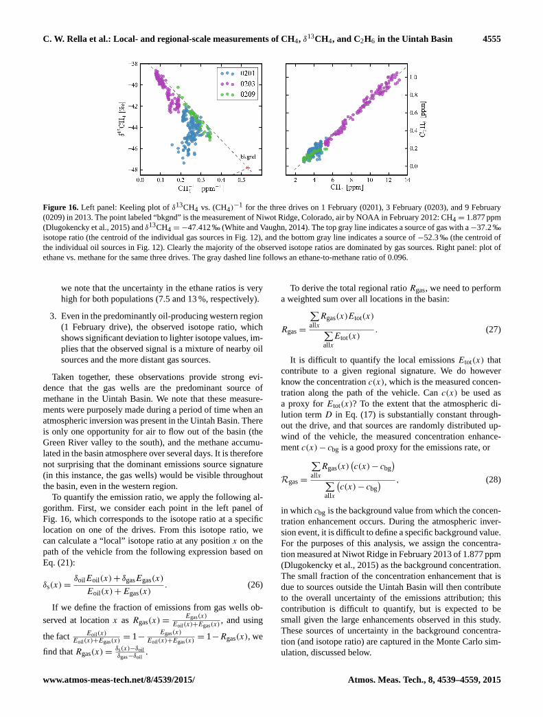
C. W. Rella et al.: Local- and regional-scale measurements of CH4, δ13CH4, and C2H6 in the Uintah Basin 4555
Figure 16. Left panel: Keeling plot of δ13CH4 vs. (CH4)−1 for the three drives on 1 February (0201), 3 February (0203), and 9 February
(0209) in 2013. The point labeled “bkgnd” is the measurement of Niwot Ridge, Colorado, air by NOAA in February 2012: CH4 = 1.877 ppm
(Dlugokencky et al., 2015) and δ13CH4 =−47.412 ‰ (White and Vaughn, 2014). The top gray line indicates a source of gas with a−37.2 ‰
isotope ratio (the centroid of the individual gas sources in Fig. 12), and the bottom gray line indicates a source of −52.3 ‰ (the centroid of
the individual oil sources in Fig. 12). Clearly the majority of the observed isotope ratios are dominated by gas sources. Right panel: plot of
ethane vs. methane for the same three drives. The gray dashed line follows an ethane-to-methane ratio of 0.096.
we note that the uncertainty in the ethane ratios is very
high for both populations (7.5 and 13 %, respectively).
3. Even in the predominantly oil-producing western region
(1 February drive), the observed isotope ratio, which
shows significant deviation to lighter isotope values, im-
plies that the observed signal is a mixture of nearby oil
sources and the more distant gas sources.
Taken together, these observations provide strong evi-
dence that the gas wells are the predominant source of
methane in the Uintah Basin. We note that these measure-
ments were purposely made during a period of time when an
atmospheric inversion was present in the Uintah Basin. There
is only one opportunity for air to flow out of the basin (the
Green River valley to the south), and the methane accumu-
lated in the basin atmosphere over several days. It is therefore
not surprising that the dominant emissions source signature
(in this instance, the gas wells) would be visible throughout
the basin, even in the western region.
To quantify the emission ratio, we apply the following al-
gorithm. First, we consider each point in the left panel of
Fig. 16, which corresponds to the isotope ratio at a specific
location on one of the drives. From this isotope ratio, we
can calculate a “local” isotope ratio at any position x on the
path of the vehicle from the following expression based on
Eq. (21):
δs(x)=δoilEoil(x)+ δgasEgas(x)
Eoil(x)+Egas(x). (26)
If we define the fraction of emissions from gas wells ob-
served at location x as Rgas(x)=Egas(x)
Eoil(x)+Egas(x), and using
the factEoil(x)
Eoil(x)+Egas(x)= 1−
Egas(x)
Eoil(x)+Egas(x)= 1−Rgas(x), we
find that Rgas(x)=δs(x)−δoil
δgas−δoil.
To derive the total regional ratio Rgas, we need to perform
a weighted sum over all locations in the basin:
Rgas =
∑allx
Rgas(x)Etot(x)∑allx
Etot(x). (27)
It is difficult to quantify the local emissions Etot(x) that
contribute to a given regional signature. We do however
know the concentration c(x), which is the measured concen-
tration along the path of the vehicle. Can c(x) be used as
a proxy for Etot(x)? To the extent that the atmospheric di-
lution term D in Eq. (17) is substantially constant through-
out the drive, and that sources are randomly distributed up-
wind of the vehicle, the measured concentration enhance-
ment c(x)− cbg is a good proxy for the emissions rate, or
Rgas =
∑allx
Rgas(x)(c(x)− cbg
)∑allx
(c(x)− cbg
) , (28)
in which cbg is the background value from which the concen-
tration enhancement occurs. During the atmospheric inver-
sion event, it is difficult to define a specific background value.
For the purposes of this analysis, we assign the concentra-
tion measured at Niwot Ridge in February 2013 of 1.877 ppm
(Dlugokencky et al., 2015) as the background concentration.
The small fraction of the concentration enhancement that is
due to sources outside the Uintah Basin will then contribute
to the overall uncertainty of the emissions attribution; this
contribution is difficult to quantify, but is expected to be
small given the large enhancements observed in this study.
These sources of uncertainty in the background concentra-
tion (and isotope ratio) are captured in the Monte Carlo sim-
ulation, discussed below.
www.atmos-meas-tech.net/8/4539/2015/ Atmos. Meas. Tech., 8, 4539–4559, 2015
4556 C. W. Rella et al.: Local- and regional-scale measurements of CH4, δ13CH4, and C2H6 in the Uintah Basin
If we continue to use the assumption that the emissions-
weighted end members of gas and oil sources are −37.2 and
−57.3 ‰, respectively, we find that the overall emission ra-
tio derived from each of the drives using Eq. (28) is 73, 93,
and 91 % for each of the three drives (1, 3, and 9 Febru-
ary 2013). If each of the drives is weighted equally, we find
thatRgas = 0.88. Alternatively, we take advantage of the fact
that we drove certain segments of the drive on multiple days
by adjusting the concentrations such that the observed con-
centration on all the drives are the same in these common
segments of the paths. In that situation, Rgas = 0.85 where
the weighting factors for the three drives are 2.2, 1.0, and 3.6,
respectively. Although the difference between the two results
is small, we will use adopt this weighting in the uncertainty
discussion below.
It is not a surprising result that the majority of methane
emissions in the Uintah Basin are from natural gas wells. The
2012 emission study performed in the Uintah (Karion et al.,
2013) focused on the gas-producing eastern portion of the
basin, but about 1000 of the 3000 oil wells in the basin. The
western portion of the flight path used in that study traverses
the western oil-producing region. This segment of the flight
path does not show a significant methane enhancement, in
support of the conclusion that the gas field is the dominant
source of methane in the region.
To quantify the uncertainty in the fractional emissions
estimate, we perform a Monte Carlo uncertainty analysis,
by varying the following parameters (normally distributed)
around their nominal values: δgas, δoil, δbkgnd, and cbkgnd. In
Karion et al. (2013), no dominant single source of methane
was found, in support of the idea that the emissions are due
to an ensemble of many sources. We have thus assumed that
the individual sources sampled directly are representative of
the distribution of sources that comprise the total emissions.
The variability in the gas and oil end members is given by
the uncertainty in the means of each individual source dis-
tributions shown in Fig. 12, orσstd√N
(Bevington and Robin-
son, 1969), assuming that the population of wells sampled
is representative of all the wells contributing to the emis-
sions. In addition, we have assumed an uncertainty in δbkgnd
and cbkgnd of 1 ‰ and 0.1 ppm, respectively; the primary
source of the uncertainty in the background parameter is
due to the fact that because of the atmospheric inversion,
it is not possible to define a clear background for the re-
gional enhancements. For this set of parameters, we find that
Rgas = 0.85± 0.07 (1-σ ), where 95 % of the Monte Carlo
realizations have Rgas > 0.75. The contributions of δgas and
δbkgnd to the total uncertainty are approximately equal, and
together account for 90 % of the total uncertainty of 0.07.
If the isotope ratios of the sources sampled are not repre-
sentative of the emissions-weighted distribution of well sig-
natures, then uncertainty in the mean of the sampled distribu-
tion underestimates the uncertainty in the centroid of the full
population. The uncertainty in the end members should be in-
creased to encompass the populations that were not sampled.
Assuming that the population is at least somewhat represen-
tative, and noting that the observed range in isotope values
and ethane ratios is typical of oil- and gas-producing geo-
logical formations, then the standard deviation of the sam-
pled distribution should represent a reasonable upper limit
for the uncertainty. In this situation, a substantial fraction of
the Monte Carlo realizations are nonphysical i.e., the isotope
ratios observed in the regional sampling can exceed the sim-
ulated gas well end member, leading to calculated emission
ratios that exceed 1 at times. However, even with these highly
uncertain end member populations, > 98 % of the realizations
predict thatRgas > 0.5, and 80 % of the realizations indicate
thatRgas > 0.7.
Finally, we note that the three drives that contributed to
this study are not necessarily representative of the total air
mass in the basin. We can obtain one estimate of this sam-
pling uncertainty by noting that the drive in the oil-producing
region lead to an estimate of 73 % for the emission ratio, and
drives in the gas-producing region lead to estimates of 93 and
91 %, for a total span of about ±10 % at most.
4 Summary
In this paper, we present a comprehensive approach to emis-
sions attribution, using an innovative CH4, δ13CH4, and
C2H6 instrument based on cavity ring-down spectroscopy
(CRDS). The design and performance of the analyzer is pre-
sented in detail. We have demonstrated that with proper cali-
bration, the instrument can deliver high-quality δ13CH4 mea-
surements with a precision that is comparable to isotope ratio
mass spectrometry. The instrument is compact and rugged,
and can be deployed in remote field stations or mobile plat-
forms with a minimal amount of user attention.
As an example of the type of research that can be per-
formed with this instrument, field measurements were per-
formed in the Uintah Basin (Utah, USA) in the winter of
2013, using a mobile lab equipped with the CRDS analyzer, a
high-accuracy GPS, a sonic anemometer, and an onboard gas
storage and playback system. With an extremely small pop-
ulation and almost no other sources of methane and ethane
other than oil and gas extraction activities, the Uintah Basin
represents an ideal location to investigate and validate new
measurement methods of atmospheric methane and ethane.
We present the results of measurements of the fugitive emis-
sions from 23 natural gas wells and six oil wells in the region.
The δ13CH4 and C2H6 signatures that we observe are consis-
tent with the signatures present in the ground. Furthermore,
regional measurements of the atmospheric CH4, δ13CH4, and
C2H6 signatures throughout the basin have been made, us-
ing continuous atmospheric sampling into a 450 m long tube.
These measurements suggest that 85±7 % of the total emis-
sions in the basin are from natural gas production.
Atmos. Meas. Tech., 8, 4539–4559, 2015 www.atmos-meas-tech.net/8/4539/2015/
C. W. Rella et al.: Local- and regional-scale measurements of CH4, δ13CH4, and C2H6 in the Uintah Basin 4557
The Supplement related to this article is available online
at doi:10.5194/amt-8-4539-2015-supplement.
Acknowledgements. The authors would like to thank
Colm Sweeney, Gaby Petron, Anna Karion, Sonja Wolter,
Tim Newberger, and Bruce Vaughn for experimental support and
helpful scientific discussions during this project.
Edited by: M. Hamilton
References
Allan, D. W.: Statistics of atomic frequency standards, P. IEEE, 54,
221–230, 1966.
Alvarez, R. A., Pacalab, S. W., Winebrake, J. J., Chameides, W. L.,
and Hamburg, S. P.: Greater focus needed on methane leakage
from natural gas infrastructure, P. Natl. Acad. Sci. USA, 109,
6435–6440, doi:10.1073/pnas.1202407109, 2012.
Bevington, P. R. and Robinson, D. K.: Data Reduction and Error
Analysis for the Physical Sciences, vol. 336, McGraw-Hill, New
York, 1969.
Bräunlich, M., Aballain, O., Marik, T., Jöckel, P., Brenninkmei-
jer, C. A., Chappellaz, J., and Sturges, W. T.: Changes in the
global atmospheric methane budget over the last decades inferred
from 13C and D isotopic analysis of Antarctic firn air, J. Geo-
phys. Res.-Atmos., 106, 20465–20481, 2001.
Chen, H., Winderlich, J., Gerbig, C., Hoefer, A., Rella, C. W.,
Crosson, E. R., Van Pelt, A. D., Steinbach, J., Kolle, O., Beck, V.,
Daube, B. C., Gottlieb, E. W., Chow, V. Y., Santoni, G. W., and
Wofsy, S. C.: High-accuracy continuous airborne measurements
of greenhouse gases (CO2 and CH4) using the cavity ring-down
spectroscopy (CRDS) technique, Atmos. Meas. Tech., 3, 375–
386, doi:10.5194/amt-3-375-2010, 2010.
Coplen, T. B., Brand, W. A., Gehre, M., Gröning, M., Meijer, H. A.,
Toman, B., and Verkouteren, R. M.: After two decades a second
anchor for the VPDB δ13C scale, Rapid Commun. Mass Sp., 20,
3165–3166, 2006.
Crosson, E. R.: A cavity ring-down analyzer for measuring atmo-
spheric levels of methane, carbon dioxide, and water vapor, Appl.
Phys. B-Lasers O., 92, 403–408, doi:10.1007/s00340-008-3135-
y, 2008.
Dlugokencky, E. J., Nisbet, E. G., Fisher, R., and Lowry, D.:
Global atmospheric methane: budget, changes and dangers, Phi-
los. Trans. Roy. Soc. London A, 369, 2058–2072, 2011.
Dlugokencky, E. J., Lang, P. M., Crotwell, A. M., Masarie, K. A.,
and Crotwell, M. J.: Atmospheric Methane Dry Air Mole
Fractions from the NOAA ESRL Carbon Cycle Cooperative
Global Air Sampling Network 1983–2014, Version: 2015-08-03,
available at: ftp://aftp.cmdl.noaa.gov/data/trace_gases/ch4/flask/
surface/, last access: 7 September, 2015.
Edwards, P. M., Young, C. J., Aikin, K., deGouw, J., Dubé, W. P.,
Geiger, F., Gilman, J., Helmig, D., Holloway, J. S., Kercher, J.,
Lerner, B., Martin, R., McLaren, R., Parrish, D. D., Peischl, J.,
Roberts, J. M., Ryerson, T. B., Thornton, J., Warneke, C.,
Williams, E. J., and Brown, S. S.: Ozone photochemistry in an
oil and natural gas extraction region during winter: simulations
of a snow-free season in the Uintah Basin, Utah, Atmos. Chem.
Phys., 13, 8955–8971, doi:10.5194/acp-13-8955-2013, 2013.
Fang, S.-X., Zhou, L.-X., Masarie, K. A., Xu, L., and Rella, C. W.:
Study of atmospheric CH4 mole fractions at three WMO/GAW
stations in China, J. Geophys. Res.-Atmos., 118, 4874–4886,
doi:10.1002/jgrd.50284, 2013.
Fisher, R., Lowry, D., Wilkin, O., Sriskantharajah, S., and Nisbet,
E. G.: High-precision, automated stable isotope analysis of at-
mospheric methane and carbon dioxide using continuous-flow
isotope-ratio mass spectrometry. Rapid Comm. Mass Spectr., 20,
200–208, 2006.
Fisher, R. E., Sriskantharajah, S., Lowry, D., Lanoisellé, M.,
Fowler, C. M. R., James, R. H., Hermansen, O., Myhre, C.
L., Stohl, A., Greinert, J., Nisbet-Jones, P. B. R., Mienert,
J., and Nisbet, E. G.: Arctic methane sources: Isotopic evi-
dence for atmospheric inputs, Geophys. Res. Lett., 38, L21803,
doi:10.1029/2011GL049319, 2011.
Kai, F. M., Tyler, S. C., Randerson, J. T., and Blake, D. R.: Reduced
methane growth rate explained by decreased Northern Hemi-
sphere microbial sources, Nature, 476, 194-197, 2011.
Karion, A., Sweeney, C., Tans, P., and Newberger, T.: AirCore:
an innovative atmospheric sampling system, J. Atmos. Ocean.
Tech., 27, 1839–1853, 2010.
Karion, A., Sweeney, C., Pétron, G., Frost, G., Hardesty, R. M.,
Kofler, J., Miller, B. R., Newberger, T., Wolter, S., Banta, R.,
Brewer, A., Dlugokencky, E., Lang, P., Montzka, S. A.,
Schnell, R., Tans, P., Trainer, M., Zamora, R., and Conley, S.:
Methane emissions estimate from airborne measurements over
a western United States natural gas field, Geophys. Res. Lett.,
40, 4393–4397, doi:10.1002/grl.50811, 2013.
Kirschke, S., Bousquet, P., Ciais, P., Saunois, M., Canadell, J. G.,
Dlugokencky, E. J., Bergamaschi, P., Bergmann, D., Blake, D. R.,
Bruhwiler, L., Cameron-Smith, P., Castaldi, S., Chevallier, F.,
Feng, L., Fraser, A., Heimann, M., Hodson, E. L., Houweling, S.,
Josse, B., Fraser, P. J., Krummel, P. B., Lamarque, J.-F., Langen-
felds, R. L., Le Quéré, C., Naik, V., O’Doherty, S., Palmer, P. I.,
Pison, I., Plummer, D., Poulter, B., Prinn, R. G., Rigby, M.,
Ringeval, B., Santini, M., Schmidt, M., Shindell, D. T., Simp-
son, I. J., Spahni, R., Steele, L. P., Strode, S. A., Sudo, K.,
Szopa, S., van der Werf, G. R., Voulgarakis, A., van Weele, M.,
Weiss, R. F., Williams, J. E., and Zeng, G.: Three decades of
global methane sources and sinks, Nat. Geosci., 6, 813–823,
2013.
Levin, I., Glatzel-Mattheier, H., Marik, T., Cuntz, M., Schmidt, M.,
and Worthy, D. E.: Verification of German methane emis-
sion inventories and their recent changes based on atmo-
spheric observations, J. Geophys. Res., 104, 3447–3456,
doi:10.1029/1998JD100064, 1999.
Lowe, D., White, J., Levin, I., Bergamaschi, P., Wahlen, M.,
and Miller, J.: Isotope measurement techniques for atmospheric
methane, in: Stable isotope measurement techniques for atmo-
spheric greenhouse gases, International Atomic Energy Agency
(IAEA), Vienna, Austria, 25–46, 2002.
Lowry, D., Holmes, C. W., Rata, N. D., O’Brien, P., and Nisbet, E.
G.: London methane emissions: Use of diurnal changes in con-
centration and δ13C to identify urban sources and verify invento-
ries, J. Geophys. Res.-Atmos., 106, 7427–7448, 2001.
www.atmos-meas-tech.net/8/4539/2015/ Atmos. Meas. Tech., 8, 4539–4559, 2015
4558 C. W. Rella et al.: Local- and regional-scale measurements of CH4, δ13CH4, and C2H6 in the Uintah Basin
Marrero, T. R. and Mason, E. A.: Gaseous diffusion coefficients, J.
Phys. Chem. Ref. Data, 1, 3–118, 1972.
Mikaloff Fletcher, S. E., Tans, P. P., Bruhwiler, L. M., Miller, J. B.,
and Heimann, M.: CH4 sources estimated from atmospheric ob-
servations of CH4 and its 13C/12C isotopic ratios: 1. Inverse
modeling of source processes, Global Biogeochem. Cy., 18,
GB4004, doi:10.1029/2004GB002223, 2004a.
Mikaloff Fletcher, S. E., Tans, P. P., Bruhwiler, L. M., Miller, J. B.,
and Heimann, M.: CH4 sources estimated from atmospheric ob-
servations of CH4 and its 13C/12C isotopic ratios: 2. Inverse
modeling of CH4 fluxes from geographical regions, Global Bio-
geochem. Cy., 18, GB4005, doi:10.1029/2004GB002224, 2004b.
Miller, J. B. and Tans, P. P.: Calculating isotopic fractionation from
atmospheric measurements at various scales, Tellus B, 55, 207–
214, 2003.
Mischler, J. A., Sowers, T. A., Alley, R. B., Battle, M.,
McConnell, J. R., Mitchell, L., Popp, T., Sofen, E., and
Spencer, M. K.: Carbon and hydrogen isotopic composition of
methane over the last 1000 years, Global Biogeochem. Cy., 23,
GB4024, doi:10.1029/2009GB003460, 2009.
Myhre, G., Shindell, D., Bréon, F.-M., Collins, W., Fuglestvedt, J.,
Huang, J., Koch, D., Lamarque, J.-F., Lee, D., Mendoza, B.,
Nakajima, T., Robock, A., Stephens, G., Takemura, T., and
Zhang, H.: Anthropogenic and natural radiative forcing, in: Cli-
mate Change 2013: the Physical Science Basis. Contribution of
Working Group I to the Fifth Assessment Report of the Intergov-
ernmental Panel on Climate Change, edited by: Stocker, T. F.,
Qin, D., Plattner, G.-K., Tignor, M., Allen, S. K., Boschung, J.,
Nauels, A., Xia, Y., Bex, V., and Midgley, P. M., Cambridge Uni-
versity Press, Cambridge, UK, New York, NY, USA, 659–740,
2013.
Nara, H., Tanimoto, H., Tohjima, Y., Mukai, H., Nojiri, Y.,
Katsumata, K., and Rella, C. W.: Effect of air composition
(N2, O2, Ar, and H2O) on CO2 and CH4 measurement by
wavelength-scanned cavity ring-down spectroscopy: calibration
and measurement strategy, Atmos. Meas. Tech., 5, 2689–2701,
doi:10.5194/amt-5-2689-2012, 2012.
Pataki, D. E., Ehleringer, J. R., Flanagan, L. B., Yakir, D., Bowl-
ing, D. R., Still, C. J., Buchmann, N., Kaplan, J. O., and Berry, J.
A.: The application and interpretation of Keeling plots in terres-
trial carbon cycle research, Global Biogeochem. Cy., 17, 1022,
doi:10.1029/2001GB001850, 2003.
Pétron, G., Frost, G., Miller, B. R., Hirsch, A. I., Montzka, S. A.,
Karion, A., Trainer, M., Sweeney, C., Andrews, A. E., Miller, L.,
Kofler, J., Bar-Ilan, A., Dlugokencky, E. J., Patrick, L., Moore
Jr., C. T., Ryerson, T. B., Siso, C., Kolodzey, W., Lang, P.
M., Conway, T., Novelli, P., Masarie, K., Hall, B., Guenther,
D., Kitzis, D., Miller, J., Welsh, D., Wolfe, D., Neff, W., and
Tans, P.: Hydrocarbon emissions characterization in the Col-
orado Front Range: a pilot study, J. Geophys. Res., 117, D04304,
doi:10.1029/2011JD016360, 2012.
Pétron, G., Karion, A., Sweeney, C., Miller, B. R., Montzka, S.
A., Frost, G. J., Trainer, M., Tans, P., Andrews, A., Kofler,
J., Helmig, D., Guenther, D., Dlugokencky, E.,. Lang, P, New-
berger, T., Wolter, S., Hall, B., Novelli, P., Brewer, A., Conley,
S., Hardesty, M., Banta, R., White, A., Noone, D.„ Wolfe, and
Schnell, R.: A new look at methane and nonmethane hydrocar-
bon emissions from oil and natural gas operations in the Col-
orado Denver–Julesburg Basin, J. Geophys. Res.-Atmos., 119,
6836–6852, doi:10.1002/2013JD021272, 2014.
Press, W. H., Flannery, B. P., Teukolsky, S. A., and Vetterling, W. T.:
Numerical Recipes: the Art of Scientific Computing, Cambridge
University Press, Cambridge, 523ff., 1986.
Quantum, G. I. S. Development Team: Quantum GIS Geographic
Information System, Open Source Geospatial Foundation, avail-
able at: http://www.qgis.org/wiki/Developers_Manual, 2013.
Quay, P. D., King, S. L., Lansdown, J. M., and Wilbur, D. O.:
Isotopic composition of methane released from wetlands: im-
plications for the increase in atmospheric methane, Global Bio-
geochem. Cy., 2, 385–397, 1988.
Rella, C. W., Chen, H., Andrews, A. E., Filges, A., Gerbig, C.,
Hatakka, J., Karion, A., Miles, N. L., Richardson, S. J., Stein-
bacher, M., Sweeney, C., Wastine, B., and Zellweger, C.: High
accuracy measurements of dry mole fractions of carbon diox-
ide and methane in humid air, Atmos. Meas. Tech., 6, 837–860,
doi:10.5194/amt-6-837-2013, 2013.
Rice, D. D., Fouch, T. D., and Johnson, R. C.: Influence of source
rock type, thermal maturity, and migration on composition and
distribution of natural gases, in: Hydrocarbon and mineral re-
sources of the Uinta Basin, Utah and Colorado, edited by: Fouch,
T. D., Vito F. N., and Chidsey Jr., T. C., Utah Geological Associ-
ation Guidebook, 20, 95–110, 1992.
Richardson, S. J., Miles, N. L., Davis, K. J., Crosson, E. R.,
Rella, C. W., and Andrews, A. E.: Field testing of cavity ring-
down spectroscopy analyzers measuring carbon dioxide and wa-
ter vapor, J. Atmos. Ocean. Tech., 29, 397–406, 2012.
Rothman, L. S., Gordon, I. E., Babikov, Y., Barbe, A., Chris Benner,
D., Bernath, P. F., Birk, M., Bizzocchi, L., Boudon, V., Brown,
L. R., Campargue, A., Chance, K., Cohen, E. A., Coudert, L.
H., Devi, V. M., Drouin, B. J.,. Fayt, A, Flaud, J.-M., Gamache,
R. R., Harrison, J. J.,. Hartmann, J.-M, Hill, C., Hodges, J. T.,
Jacquemart, D., Jolly, A., Lamouroux, J., Le Roy, R. J., Li,
G., Long, D. A., Lyulin, O. M., Mackie, C. J., Massie, S. T.,
Mikhailenko, S., Müller, H. S. P., Naumenko, O. V., Nikitin,
A. V., Orphal, J., Perevalov, V.,. Perrin, A., Polovtseva, E. R.,
Richard, C., Smith, M. A. H., Starikova, E., Sung, K., Tashkun,
S., Tennyson, J., Toon, G. C., Tyuterev, V. G., and Wagner, G.:
The HITRAN2012 molecular spectroscopic database, J. Quant.
Spectrosc. Ra., 130, 4–50, 2013.
Schnell, R. C., Oltmans, S. J., Johnson, B. J., and Neely III, R. R.:
The Anatomy of Wintertime Photochemical Ozone Production
Events in the Upper Green River, WY and Uintah, UT Natu-
ral Gas Fields, in: AGU Fall Meeting Abstracts, San Francisco,
USA, 3–7 December 2012, Vol. 1, p. 5, 2012.
Schoell, M.: The hydrogen and carbon isotopic composition of
methane from natural gases of various origins, Geochim. Cos-
mochim. Ac., 44, 649–661, doi:10.1016/0016-7037(80)90155-6,
1980.
Simpson, I. J., Andersen, M. P. S., Meinardi, S., Bruh-
wiler, L., Blake, N. J., Helmig, D., Sherwood Rowland, F., and
Blake, D. R.: Long-term decline of global atmospheric ethane
concentrations and implications for methane, Nature, 488, 490–
494, 2012.
Smith, L. K., Lewis Jr., W. M., Chanton, J. P., Cronin, G., and
Hamilton, S. K.: Methane emissions from the Orinoco River
floodplain, Venezuela, Biogeochemistry, 51, 113–140, 2000.
Atmos. Meas. Tech., 8, 4539–4559, 2015 www.atmos-meas-tech.net/8/4539/2015/
C. W. Rella et al.: Local- and regional-scale measurements of CH4, δ13CH4, and C2H6 in the Uintah Basin 4559
Tans, P. P.: US Patent No. 7,597,014, US Patent and Trademark Of-
fice, Washington, DC, 2009.
UBETS Report: Final Report: Uintah Basin Energy and Trans-
portation Study, available at: www.utssd.utah.gov/documents/
ubetsreport.pdf (last access: 18 June 2014), 2013.
Uintah Map: Uintah County Oil and Gas Wells, created
4/16/2013, available at: http://www.co.uintah.ut.us/gis/Oil%
20and%20Gas%20Wells.pdf (last access: 4 July 2014), 2013.
Utah Well Information Query: State of Utah Department of Nat-
ural Resources Division of Oil Gas and Mining, Well Informa-
tion Query, available at: http://oilgas.ogm.utah.gov/Data_Center/
LiveData_Search/well_information.htm (last access: February
2013), 2012.
Varghese, P. L. and Hanson, R. K.: Collisional narrowing effects on
spectral line shapes measured at high resolution, Appl. Optics,
23, 2376–2385, doi:10.1364/AO.23.002376, 1984.
Werner, R. A. and Brand, W. A.: Referencing strategies and tech-
niques in stable isotope ratio analysis, Rapid Commun. Mass Sp.,
15, 501–519, 2001.
White, J. W. C. and Vaughn, B. H.: Stable Isotopic Composition
of Atmospheric Methane (13C) from the NOAA ESRL Carbon
Cycle Cooperative Global Air Sampling Network, 1998–2014,
Version: 2015-08-03, University of Colorado, Institute of Arctic
and Alpine Research (INSTAAR), available at: ftp://aftp.cmdl.
noaa.gov/data/trace_gases/ch4c13/flask/, last access: 7 Septem-
ber, 2015.
Winderlich, J., Chen, H., Gerbig, C., Seifert, T., Kolle, O.,
Lavric, J. V., Kaiser, C., Höfer, A., and Heimann, M.: Con-
tinuous low-maintenance CO2/CH4/H2O measurements at the
Zotino Tall Tower Observatory (ZOTTO) in Central Siberia, At-
mos. Meas. Tech., 3, 1113–1128, doi:10.5194/amt-3-1113-2010,
2010.
Xiao, Y., Logan, J. A., Jacob, D. J., Hudman, R. C., Yantosca, R.,
and Blake, D. R.: Global budget of ethane and regional con-
straints on US sources, J. Geophys. Res.-Atmos., 113, D21306,
doi:10.1029/2007JD009415, 2008.
www.atmos-meas-tech.net/8/4539/2015/ Atmos. Meas. Tech., 8, 4539–4559, 2015