Forward thinking: the predictive approach
14
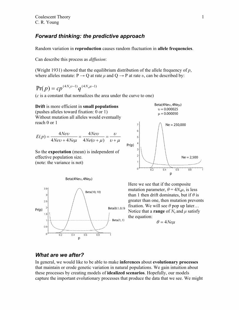
Coalescent Theory 1 C. R. Young Forward thinking: the predictive approach Random variation in reproduction causes random fluctuation in allele frequencies. Can describe this process as diffusion: (Wright 1931) showed that the equilibrium distribution of the allele frequency of p, where alleles mutate: P → Q at rate μ and Q → P at rate υ, can be described by: ) 1 4 ( ) 1 4 ( ) Pr( − − = µ υ e e N N q cp p (c is a constant that normalizes the area under the curve to one) Drift is more efficient in small populations (pushes alleles toward fixation: 0 or 1) Without mutation all alleles would eventually reach 0 or 1 µ υ υ µ υ υ µ υ υ + = + = + = ) ( 4 4 4 4 4 ) ( Ne Ne Ne Ne Ne p E So the expectation (mean) is independent of effective population size. (note: the variance is not) Here we see that if the composite mutation parameter, θ = 4N e μ, is less than 1 then drift dominates, but if θ is greater than one, then mutation prevents fixation. We will see θ pop up later… Notice that a range of N e and μ satisfy the equation: µ θ Ne 4 = What are we after? In general, we would like to be able to make inferences about evolutionary processes that maintain or erode genetic variation in natural populations. We gain intuition about these processes by creating models of idealized scenarios. Hopefully, our models capture the important evolutionary processes that produce the data that we see. We might
Transcript of Forward thinking: the predictive approach
Coalescent Theory 1 C. R. Young
Forward thinking: the predictive approach Random variation in reproduction causes random fluctuation in allele frequencies. Can describe this process as diffusion: (Wright 1931) showed that the equilibrium distribution of the allele frequency of p, where alleles mutate: P → Q at rate µ and Q → P at rate υ, can be described by:
)14()14()Pr( −−= µυ ee NN qcpp (c is a constant that normalizes the area under the curve to one) Drift is more efficient in small populations (pushes alleles toward fixation: 0 or 1) Without mutation all alleles would eventually reach 0 or 1
µυυ
µυυ
µυυ
+=
+=
+=
)(44
444)(
NeNe
NeNeNepE
So the expectation (mean) is independent of effective population size. (note: the variance is not)
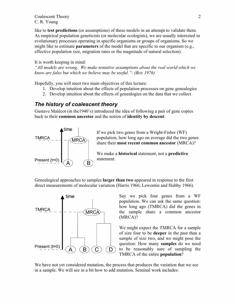
Here we see that if the composite mutation parameter, θ = 4Neµ, is less than 1 then drift dominates, but if θ is greater than one, then mutation prevents fixation. We will see θ pop up later… Notice that a range of Ne and µ satisfy the equation:
µθ Ne4=
What are we after? In general, we would like to be able to make inferences about evolutionary processes that maintain or erode genetic variation in natural populations. We gain intuition about these processes by creating models of idealized scenarios. Hopefully, our models capture the important evolutionary processes that produce the data that we see. We might
Coalescent Theory 2 C. R. Young
like to test predictions (or assumptions) of these models in an attempt to validate them. As empirical population geneticists (or molecular ecologists), we are usually interested in evolutionary processes operating in specific organisms or groups of organisms. So we might like to estimate parameters of the model that are specific to our organism (e.g., effective population size, migration rates or the magnitude of natural selection). It is worth keeping in mind: “All models are wrong. We make tentative assumptions about the real world which we know are false but which we believe may be useful.”- (Box 1976) Hopefully, you will meet two main objectives of this lecture:
1. Develop intuition about the effects of population processes on gene genealogies 2. Develop intuition about the effects of genealogies on the data that we collect
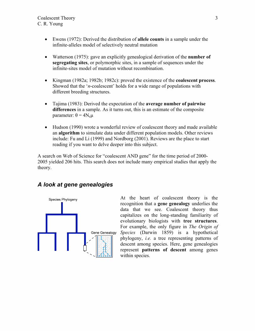
The history of coalescent theory Gustave Malécot (in the1940’s) introduced the idea of following a pair of gene copies back to their common ancestor and the notion of identity by descent:
If we pick two genes from a Wright-Fisher (WF) population, how long ago on average did the two genes share their most recent common ancestor (MRCA)? We make a historical statement, not a predictive statement.
Genealogical approaches to samples larger than two appeared in response to the first direct measurements of molecular variation (Harris 1966; Lewontin and Hubby 1966).
Say we pick four genes from a WF population. We can ask the same question: how long ago (TMRCA) did the genes in the sample share a common ancestor (MRCA)? We might expect the TMRCA for a sample of size four to be deeper in the past than a sample of size two, and we might pose the question: How many samples do we need to be reasonably sure of sampling the TMRCA of the entire population?
We have not yet considered mutation, the process that produces the variation that we see in a sample. We will see in a bit how to add mutation. Seminal work includes:
Coalescent Theory 3 C. R. Young
• Ewens (1972): Derived the distribution of allele counts in a sample under the
infinite-alleles model of selectively neutral mutation
• Watterson (1975): gave an explicitly genealogical derivation of the number of segregating sites, or polymorphic sites, in a sample of sequences under the infinite-sites model of mutation without recombination.
• Kingman (1982a; 1982b; 1982c): proved the existence of the coalescent process.
Showed that the ‘n-coalescent’ holds for a wide range of populations with different breeding structures.
• Tajima (1983): Derived the expectation of the average number of pairwise
differences in a sample. As it turns out, this is an estimate of the composite parameter: θ = 4Neµ
• Hudson (1990) wrote a wonderful review of coalescent theory and made available
an algorithm to simulate data under different population models. Other reviews include: Fu and Li (1999) and Nordborg (2001). Reviews are the place to start reading if you want to delve deeper into this subject.
A search on Web of Science for “coalescent AND gene” for the time period of 2000-2005 yielded 206 hits. This search does not include many empirical studies that apply the theory.
A look at gene genealogies
At the heart of coalescent theory is the recognition that a gene genealogy underlies the data that we see. Coalescent theory thus capitalizes on the long-standing familiarity of evolutionary biologists with tree structures. For example, the only figure in The Origin of Species (Darwin 1859) is a hypothetical phylogeny, i.e. a tree representing patterns of descent among species. Here, gene genealogies represent patterns of descent among genes within species.
Coalescent Theory 4 C. R. Young
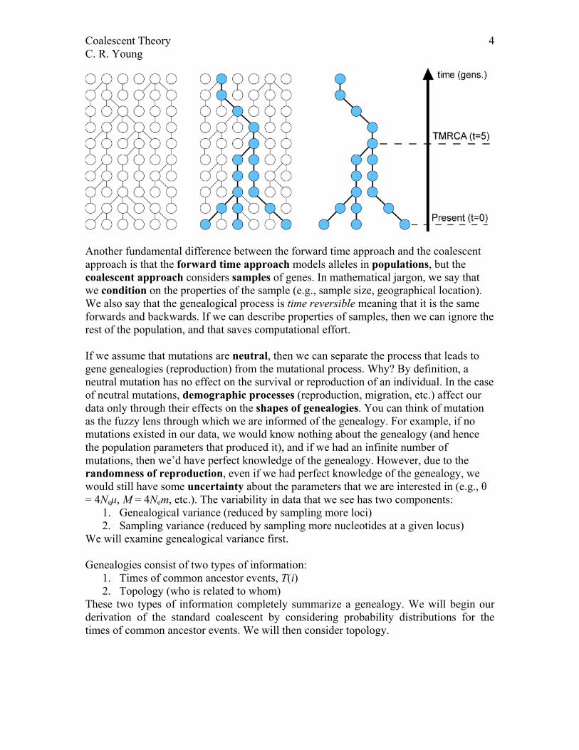
Another fundamental difference between the forward time approach and the coalescent approach is that the forward time approach models alleles in populations, but the coalescent approach considers samples of genes. In mathematical jargon, we say that we condition on the properties of the sample (e.g., sample size, geographical location). We also say that the genealogical process is time reversible meaning that it is the same forwards and backwards. If we can describe properties of samples, then we can ignore the rest of the population, and that saves computational effort. If we assume that mutations are neutral, then we can separate the process that leads to gene genealogies (reproduction) from the mutational process. Why? By definition, a neutral mutation has no effect on the survival or reproduction of an individual. In the case of neutral mutations, demographic processes (reproduction, migration, etc.) affect our data only through their effects on the shapes of genealogies. You can think of mutation as the fuzzy lens through which we are informed of the genealogy. For example, if no mutations existed in our data, we would know nothing about the genealogy (and hence the population parameters that produced it), and if we had an infinite number of mutations, then we’d have perfect knowledge of the genealogy. However, due to the randomness of reproduction, even if we had perfect knowledge of the genealogy, we would still have some uncertainty about the parameters that we are interested in (e.g., θ = 4Neµ, M = 4Nem, etc.). The variability in data that we see has two components:
1. Genealogical variance (reduced by sampling more loci) 2. Sampling variance (reduced by sampling more nucleotides at a given locus)
We will examine genealogical variance first. Genealogies consist of two types of information:
1. Times of common ancestor events, T(i) 2. Topology (who is related to whom)
These two types of information completely summarize a genealogy. We will begin our derivation of the standard coalescent by considering probability distributions for the times of common ancestor events. We will then consider topology.
Coalescent Theory 5 C. R. Young
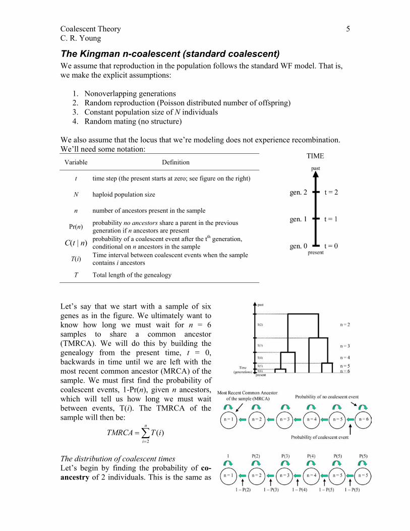
The Kingman n-coalescent (standard coalescent) We assume that reproduction in the population follows the standard WF model. That is, we make the explicit assumptions:
1. Nonoverlapping generations 2. Random reproduction (Poisson distributed number of offspring) 3. Constant population size of N individuals 4. Random mating (no structure)
We also assume that the locus that we’re modeling does not experience recombination. We’ll need some notation:
Variable Definition
t time step (the present starts at zero; see figure on the right)
N haploid population size
n number of ancestors present in the sample
Pr(n) probability no ancestors share a parent in the previous generation if n ancestors are present
C(t | n) probability of a coalescent event after the tth generation, conditional on n ancestors in the sample
T(i) Time interval between coalescent events when the sample contains i ancestors
T Total length of the genealogy
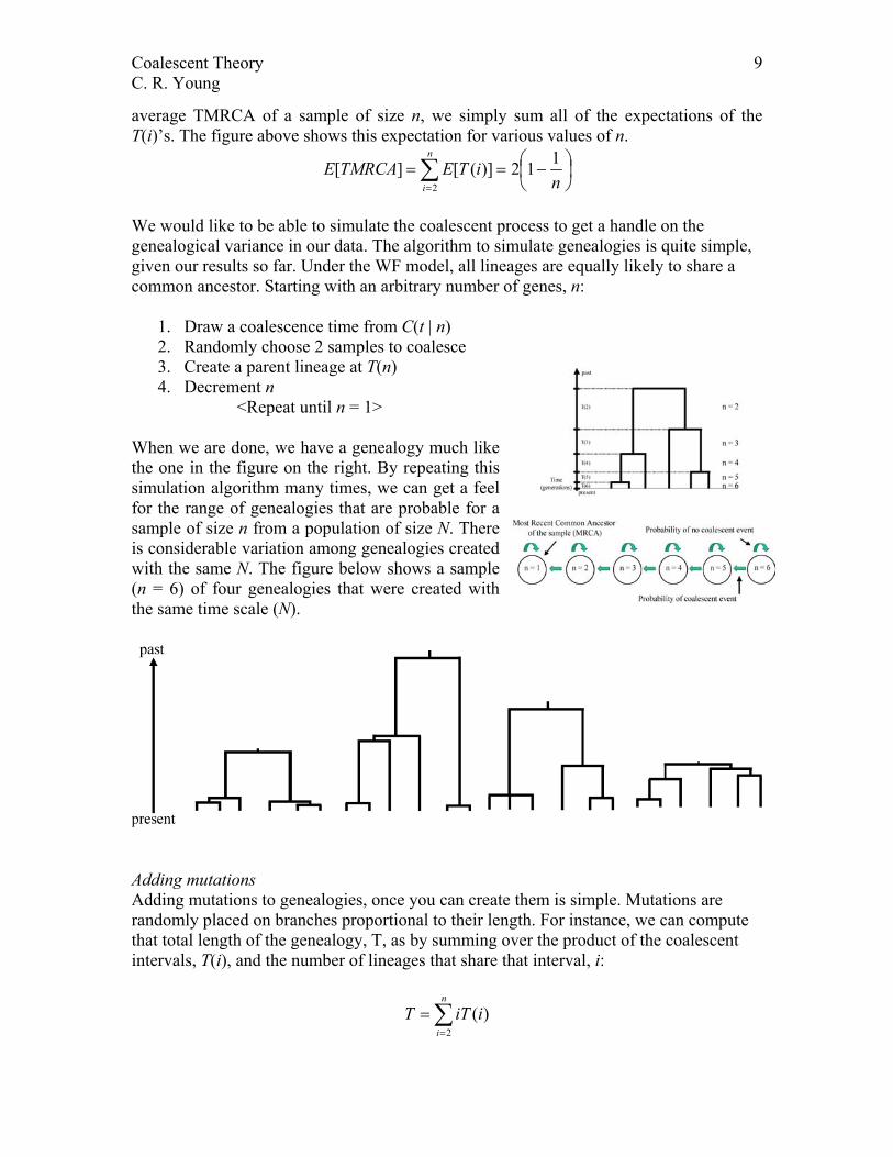
Let’s say that we start with a sample of six genes as in the figure. We ultimately want to know how long we must wait for n = 6 samples to share a common ancestor (TMRCA). We will do this by building the genealogy from the present time, t = 0, backwards in time until we are left with the most recent common ancestor (MRCA) of the sample. We must first find the probability of coalescent events, 1-Pr(n), given n ancestors, which will tell us how long we must wait between events, T(i). The TMRCA of the sample will then be:
∑=
=n
iiTTMRCA
2)(
The distribution of coalescent times Let’s begin by finding the probability of co-ancestry of 2 individuals. This is the same as
Coalescent Theory 6 C. R. Young
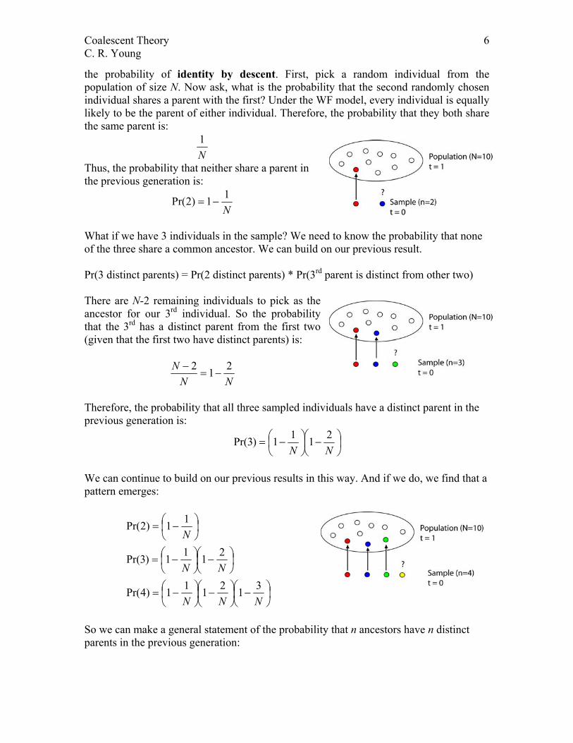
the probability of identity by descent. First, pick a random individual from the population of size N. Now ask, what is the probability that the second randomly chosen individual shares a parent with the first? Under the WF model, every individual is equally likely to be the parent of either individual. Therefore, the probability that they both share the same parent is:
N1
Thus, the probability that neither share a parent in the previous generation is:
N11)2Pr( −=
What if we have 3 individuals in the sample? We need to know the probability that none of the three share a common ancestor. We can build on our previous result. Pr(3 distinct parents) = Pr(2 distinct parents) * Pr(3rd parent is distinct from other two) There are N-2 remaining individuals to pick as the ancestor for our 3rd individual. So the probability that the 3rd has a distinct parent from the first two (given that the first two have distinct parents) is:
NNN 212
−=−
Therefore, the probability that all three sampled individuals have a distinct parent in the previous generation is:
−
−=
NN2111)3Pr(
We can continue to build on our previous results in this way. And if we do, we find that a pattern emerges:
−
−
NN
N312
2
−=
−
−=
−=
N
N
N
111)4Pr(
111)3Pr(
11)2Pr(
So we can make a general statement of the probability that n ancestors have n distinct parents in the previous generation:
Coalescent Theory 7 C. R. Young
Nnn
Nin
n
i 2)1(1)Pr(
1
1
−≈−= ∏
−
=
We have found the probability that no ancestors in a sample of size n share a common ancestor in the previous generation (one time step). Since the outcome of each generation is independent, the probability that no ancestors in a sample share a common ancestor in t generations (no coalescent event) is:
tn)Pr( The probability, C(t | n), that there is a coalescent event in the tth generation conditional on there being n lineages in the sample is:
))Pr(1()Pr()|( nnntC t −= That is, there were no coalescent events for the first t generations, with probability Pr(n)t, then there was a coalescent event in the (t+1)th generation, with probability 1-Pr(n). This looks a lot like Binomial sampling, where we have:
yx pp )1( − In our case, we have:
1)1( ppt − This is a specific type of binomial sampling where (1-p) is a very small probability and the total number of trials, t+1, must be very large for an event of type (1-p) to occur. This type of process is called a Poisson process. We know from statistical probability theory that the waiting time for a Poisson process, t, can be approximated by an exponential distribution:
tet λλ −=)Pr(
where λ is the rate parameter. In our case:N
nn2
)1( −=λ
The distribution of waiting times until a coalescent event is: t
Nnn
eN
nnntC 2)1(
2)1()|(
−−−
=
The exponential distribution has mean 1/λ.
Mean time of coalescent event for i distinct lineages: )1(
2)]([−
=ii
NiTE
Mean time of coalescent event for sample of size n = 2: NNTE =−
=)12(2
2)]2([
We have to wait N generations on average for two randomly chosen individuals to share a common ancestor. There is a large variance in waiting times (TMRCA). For a population of size N = 100, the TMRCA of a sample of size 2 will be between 5 – 300 generations about 90% of the time. Likewise, for a population of size N = 1000, the TMRCA will be between 50 – 3000 generations 90% of the time.
Coalescent Theory 8 C. R. Young
If we measure time in units of N generations, then we arrive at a general model for the times of coalescent events:
Rate of coalescent events: 2
)1( −=
nnλ
Probability of coalescent event at time, t: t
nn
ennntC 2)1(
2)1()|(
−−−
=
Mean time of coalescent event for i distinct lineages: )1(
2)]([−
=ii
iTE
Mean time of coalescent event for sample of size n = 2: 1)12(2
2)]2([ =−
=TE
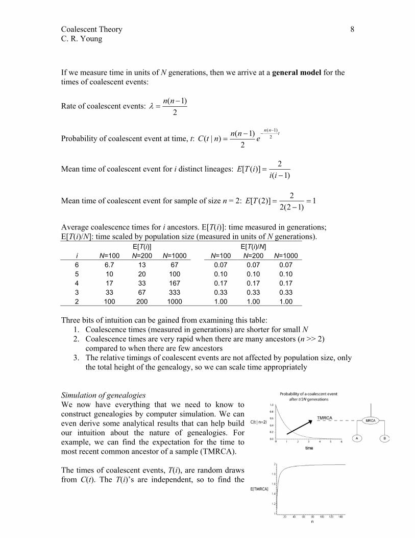
Average coalescence times for i ancestors. E[T(i)]: time measured in generations; E[T(i)/N]: time scaled by population size (measured in units of N generations). E[T(i)] E[T(i)/N]
i N=100 N=200 N=1000 N=100 N=200 N=1000 6 6.7 13 67 0.07 0.07 0.07 5 10 20 100 0.10 0.10 0.10 4 17 33 167 0.17 0.17 0.17 3 33 67 333 0.33 0.33 0.33 2 100 200 1000 1.00 1.00 1.00
Three bits of intuition can be gained from examining this table:
1. Coalescence times (measured in generations) are shorter for small N 2. Coalescence times are very rapid when there are many ancestors (n >> 2)
compared to when there are few ancestors 3. The relative timings of coalescent events are not affected by population size, only
the total height of the genealogy, so we can scale time appropriately Simulation of genealogies We now have everything that we need to know to construct genealogies by computer simulation. We can even derive some analytical results that can help build our intuition about the nature of genealogies. For example, we can find the expectation for the time to most recent common ancestor of a sample (TMRCA). The times of coalescent events, T(i), are random draws from C(t). The T(i)’s are independent, so to find the
Coalescent Theory 9 C. R. Young
average TMRCA of a sample of size n, we simply sum all of the expectations of the T(i)’s. The figure above shows this expectation for various values of n.
−== ∑
= niTETMRCAE
n
i
112)]([][2
We would like to be able to simulate the coalescent process to get a handle on the genealogical variance in our data. The algorithm to simulate genealogies is quite simple, given our results so far. Under the WF model, all lineages are equally likely to share a common ancestor. Starting with an arbitrary number of genes, n:
1. Draw a coalescence time from C(t | n) 2. Randomly choose 2 samples to coalesce 3. Create a parent lineage at T(n) 4. Decrement n
<Repeat until n = 1> When we are done, we have a genealogy much like the one in the figure on the right. By repeating this simulation algorithm many times, we can get a feel for the range of genealogies that are probable for a sample of size n from a population of size N. There is considerable variation among genealogies created with the same N. The figure below shows a sample (n = 6) of four genealogies that were created with the same time scale (N).
Adding mutations Adding mutations to genealogies, once you can create them is simple. Mutations are randomly placed on branches proportional to their length. For instance, we can compute that total length of the genealogy, T, as by summing over the product of the coalescent intervals, T(i), and the number of lineages that share that interval, i:
∑=
=n
iiiTT
2)(
Coalescent Theory 10 C. R. Young
Assuming that the per generation mutation rate is µ under the infinite-sites model, the expected number of polymorphic sites, E[S], is:
TNSE µ=][
If we define θ = 2Nµ for a haploid locus, then we see that:
∑
∑
∑
−
=
=
=
=
−=
=
1
1
2
2
1][
)1(2
2][
)(2
][
n
i
n
i
n
i
iSE
iiiSE
iiTSE
θ
θ
θ
You might recognize this equation after a bit of rearrangement:
∑−
=
= 1
1
1ˆ
n
i
S
i
Sθ
This is the estimate of genetic diversity that you saw in lecture 2, Watterson’s theta. Keep in mind that we are not limited to the infinite-sites model of mutation. In fact, we could use any model of mutation that we like. For instance, if we were interested in microsatellite data, we could use the stepwise mutation model. If we wanted to allow for homoplasy, then we could use the finite-sites model. Relaxing the assumptions of the WF model We have assumed so far that the population follows the WF model. Much of the work on coalescent theory in the past 5–10 years explores the coalescent when some of the assumptions of the WF model are relaxed. Some results have been obtained from the Moran model, which allows overlapping generations. This model results in a change in the time scaling (much like changes in N), but otherwise, they are largely the same. Other assumptions that have been relaxed include:
1. Fluctuations in population size 2. Migration/isolation models (structured coalescent) 3. Recombination (recombination graph) 4. Selection (ancestral selection graph) 5. Metapopulations (extinction/recolonization)
Coalescent Theory 11 C. R. Young
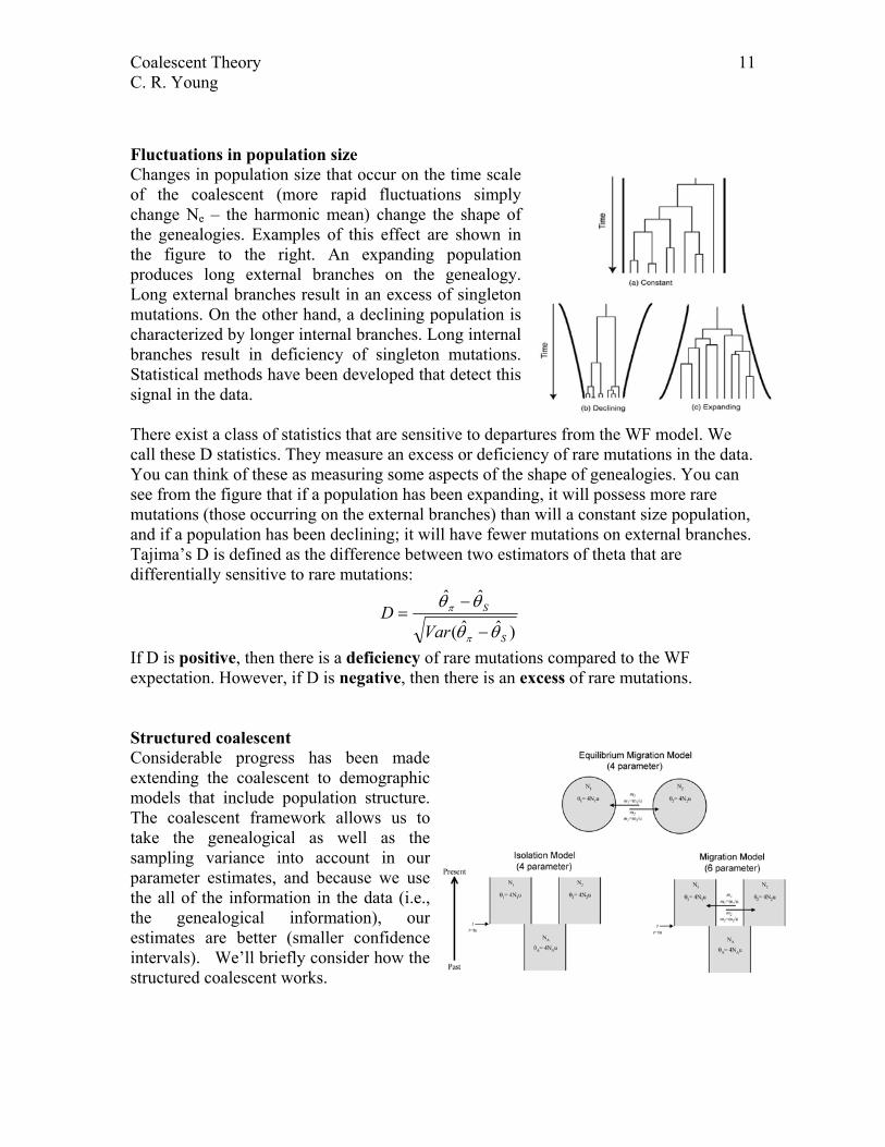
Fluctuations in population size Changes in population size that occur on the time scale of the coalescent (more rapid fluctuations simply change Ne – the harmonic mean) change the shape of the genealogies. Examples of this effect are shown in the figure to the right. An expanding population produces long external branches on the genealogy. Long external branches result in an excess of singleton mutations. On the other hand, a declining population is characterized by longer internal branches. Long internal branches result in deficiency of singleton mutations. Statistical methods have been developed that detect this signal in the data. There exist a class of statistics that are sensitive to departures from the WF model. We call these D statistics. They measure an excess or deficiency of rare mutations in the data. You can think of these as measuring some aspects of the shape of genealogies. You can see from the figure that if a population has been expanding, it will possess more rare mutations (those occurring on the external branches) than will a constant size population, and if a population has been declining; it will have fewer mutations on external branches. Tajima’s D is defined as the difference between two estimators of theta that are differentially sensitive to rare mutations:
)ˆˆ(
ˆˆ
S
S
VarD
θθ
θθ
π
π
−
−=
If D is positive, then there is a deficiency of rare mutations compared to the WF expectation. However, if D is negative, then there is an excess of rare mutations. Structured coalescent Considerable progress has been made extending the coalescent to demographic models that include population structure. The coalescent framework allows us to take the genealogical as well as the sampling variance into account in our parameter estimates, and because we use the all of the information in the data (i.e., the genealogical information), our estimates are better (smaller confidence intervals). We’ll briefly consider how the structured coalescent works.
Coalescent Theory 12 C. R. Young
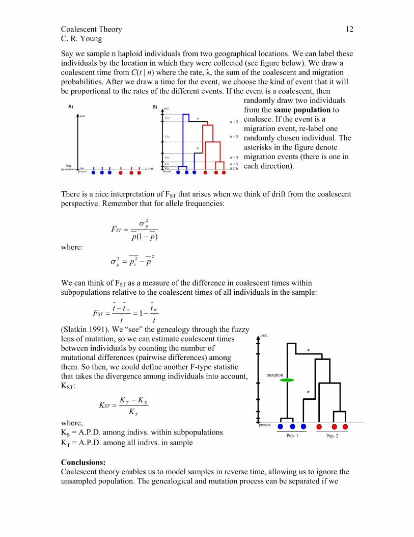
Say we sample n haploid individuals from two geographical locations. We can label these individuals by the location in which they were collected (see figure below). We draw a coalescent time from C(t | n) where the rate, λ, the sum of the coalescent and migration probabilities. After we draw a time for the event, we choose the kind of event that it will be proportional to the rates of the different events. If the event is a coalescent, then
randomly draw two individuals from the same population to coalesce. If the event is a migration event, re-label one randomly chosen individual. The asterisks in the figure denote migration events (there is one in each direction).
There is a nice interpretation of FST that arises when we think of drift from the coalescent perspective. Remember that for allele frequencies:
)1(
2
ppF p
ST−
=σ
where: 222 ppip −=σ
We can think of FST as a measure of the difference in coalescent times within subpopulations relative to the coalescent times of all individuals in the sample:
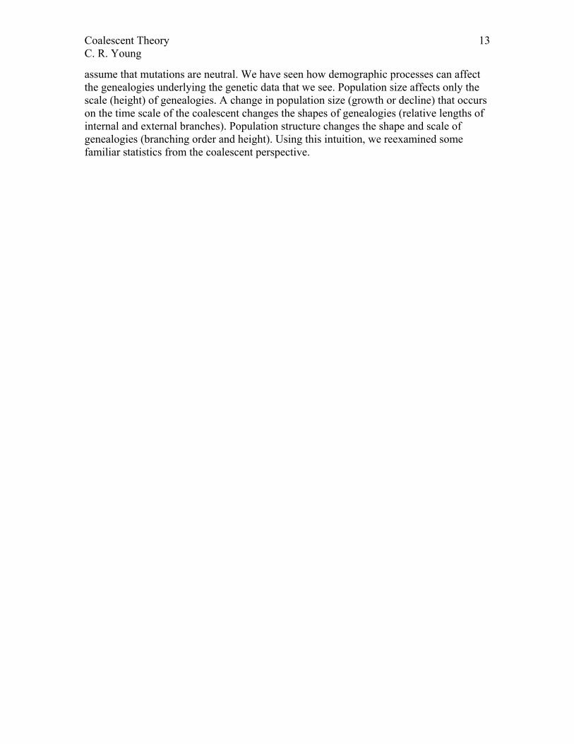
(Slatkin 1991). We “see” the genealogy through the flens of mutation, so we can estimate coalescent times between individuals by counting the number of mutational differences (pairwise differences) among them. So then, we could define another F-type statistic that takes the divergence among individuals into account, K
uzzy
ST:
tt
tttF ww
ST −=−
= 1
T
STST
KKK
K−
=
where, KS = A.P.D. among indivs. within subpopulations KT = A.P.D. among all indivs. in sample Conclusions: Coalescent theory enables us to model samples in reverse time, allowing us to ignore the unsampled population. The genealogical and mutation process can be separated if we
Coalescent Theory 13 C. R. Young
assume that mutations are neutral. We have seen how demographic processes can affect the genealogies underlying the genetic data that we see. Population size affects only the scale (height) of genealogies. A change in population size (growth or decline) that occurs on the time scale of the coalescent changes the shapes of genealogies (relative lengths of internal and external branches). Population structure changes the shape and scale of genealogies (branching order and height). Using this intuition, we reexamined some familiar statistics from the coalescent perspective.
Coalescent Theory 14 C. R. Young
References: Baker, R. J., K. S, Davis, R. D. Bradley, M. J. hamilton, and R. V. D. Bussche. 1989.
Ribosomal-DNA, mitochondrial-DNA, chromosomal, and allozymic studies on a contact zone in the pocket gopher, Geomys. Evolution 43:63-75.
Box, G. E. P. 1976. Science and statistics. Journal of the American Statistical Association 71:791-799.
Darwin, C. 1859. The origin of species Ewens, W. J. 1972. The sampling theory of selectively neutral alleles. Theor. Popul. Biol.
3:87–112. Fu, Y.-X., and W.-H. Li. 1999. Coalescing into the 21st Century: An Overview and
Prospects of Coalescent Theory. Theoretical Population Biology 56:1-10. Harris, H. 1966. Enzyme polymorphism in man. prsb 164:298-310. Hudson, R. R. 1990. Gene genealogies and the coalescent process. Oxford Surveys in
Evolutionary Biology 7:1-44. Kingman, J. F. C. 1982a. The coalescent. Stochastic Processes and Their Applications
13:235-248. Kingman, J. F. C. 1982b. Exchangeability and the evolution of large populations. Pp. 97-
112 in G. Koch and F. Spizzichino, eds. Exchangeability in Probability and Statistics. Proceedings of the International Conference on Exchangeability in Probability and Statistics, Rome, 6th-9th April, 1981, in honour of Professor Bruno de Finetti. North-Holland Elsevier, Amsterdam.
Kingman, J. F. C. 1982c. On the genealogy of large populations. Journal of Applied Probability 19A:27-43.
Lewontin, R. C., and J. L. Hubby. 1966. A molecular approach to the study of genic heterozygosity in natural populations of Drosophila pseudoobscura. Genetics 54:595-609.
Nordborg, M. 2001. Coalescent theory in D. Balding, M. Bishop and C. Cannings, eds. Handbook of Statistical Genetics. Wiley, Chichester, UK.
Slatkin, M. 1991. Inbreeding coefficients and coalescence times. grc 58:167-175. Tajima, F. 1983. Evolutionary relationships of DNA sequences in finite populations.
Genetics 105:437-460. Watterson, G. A. 1975. On the number of segregating sites in genetical models without
recombination. tpb 7:256-276. Wright, S. 1931. Evolution in Mendelian populations. Genetics 16:97-159.