Feynman Diagrams For Pedestrians - WebHomekauer/projects/scripts/ohl.pdf · Feynman Diagrams For...
50
Feynman Diagrams For Pedestrians Thorsten Ohl Institute for Theoretical Physics and Astrophysics Würzburg University http://physik.uni-wuerzburg.de/ohl 43rd Maria Laach School for High Energy Physics Spree Hotel Bautzen September 6-16, 2011 Φ T P 2 Abstract This set of interleaved lectures and exercises will (re)introduce working ex- perimental particle physicists to the techniques used for computing simple cross sections in the standard model and its extensions. The approach is deliberately pedestrian with an emphasis on real world applications. After an introduction, gradually more and more time will be spent actually computing stuff in order to build confidence and gain intuition for (new) physics signals in cross sections.
Transcript of Feynman Diagrams For Pedestrians - WebHomekauer/projects/scripts/ohl.pdf · Feynman Diagrams For...
Feynman Diagrams For Pedestrians
Thorsten OhlInstitute for Theoretical Physics and Astrophysics
Würzburg Universityhttp://physik.uni-wuerzburg.de/ohl
43rd Maria Laach School for High Energy PhysicsSpree Hotel BautzenSeptember 6-16, 2011
ΦTP2Abstract
This set of interleaved lectures and exercises will (re)introduce working ex-perimental particle physicists to the techniques used for computing simple crosssections in the standard model and its extensions. The approach is deliberatelypedestrian with an emphasis on real world applications.
After an introduction, gradually more and more time will be spent actuallycomputing stuff in order to build confidence and gain intuition for (new) physicssignals in cross sections.
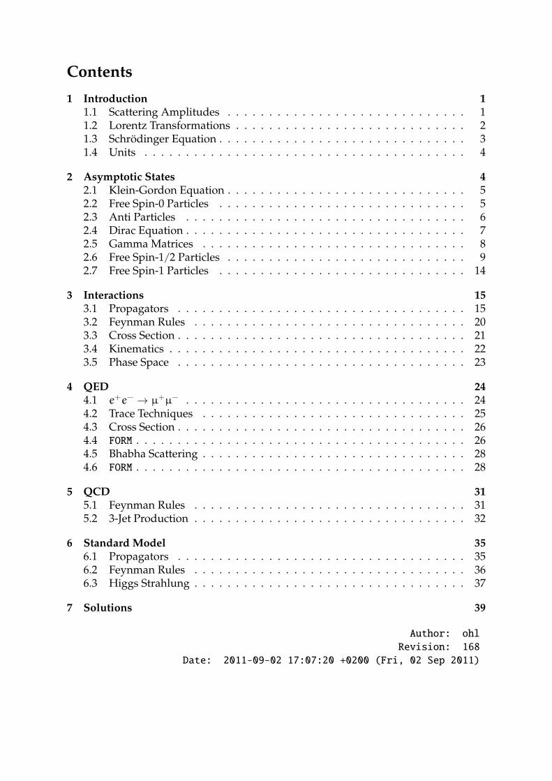
Contents
1 Introduction 11.1 Scattering Amplitudes . . . . . . . . . . . . . . . . . . . . . . . . . . . . . 11.2 Lorentz Transformations . . . . . . . . . . . . . . . . . . . . . . . . . . . . 21.3 Schrödinger Equation . . . . . . . . . . . . . . . . . . . . . . . . . . . . . . 31.4 Units . . . . . . . . . . . . . . . . . . . . . . . . . . . . . . . . . . . . . . . 4
2 Asymptotic States 42.1 Klein-Gordon Equation . . . . . . . . . . . . . . . . . . . . . . . . . . . . . 52.2 Free Spin-0 Particles . . . . . . . . . . . . . . . . . . . . . . . . . . . . . . 52.3 Anti Particles . . . . . . . . . . . . . . . . . . . . . . . . . . . . . . . . . . 62.4 Dirac Equation . . . . . . . . . . . . . . . . . . . . . . . . . . . . . . . . . . 72.5 Gamma Matrices . . . . . . . . . . . . . . . . . . . . . . . . . . . . . . . . 82.6 Free Spin-1/2 Particles . . . . . . . . . . . . . . . . . . . . . . . . . . . . . 92.7 Free Spin-1 Particles . . . . . . . . . . . . . . . . . . . . . . . . . . . . . . 14
3 Interactions 153.1 Propagators . . . . . . . . . . . . . . . . . . . . . . . . . . . . . . . . . . . 153.2 Feynman Rules . . . . . . . . . . . . . . . . . . . . . . . . . . . . . . . . . 203.3 Cross Section . . . . . . . . . . . . . . . . . . . . . . . . . . . . . . . . . . . 213.4 Kinematics . . . . . . . . . . . . . . . . . . . . . . . . . . . . . . . . . . . . 223.5 Phase Space . . . . . . . . . . . . . . . . . . . . . . . . . . . . . . . . . . . 23
4 QED 244.1 e+e− → µ+µ− . . . . . . . . . . . . . . . . . . . . . . . . . . . . . . . . . . 244.2 Trace Techniques . . . . . . . . . . . . . . . . . . . . . . . . . . . . . . . . 254.3 Cross Section . . . . . . . . . . . . . . . . . . . . . . . . . . . . . . . . . . . 264.4 FORM . . . . . . . . . . . . . . . . . . . . . . . . . . . . . . . . . . . . . . . . 264.5 Bhabha Scattering . . . . . . . . . . . . . . . . . . . . . . . . . . . . . . . . 284.6 FORM . . . . . . . . . . . . . . . . . . . . . . . . . . . . . . . . . . . . . . . . 28
5 QCD 315.1 Feynman Rules . . . . . . . . . . . . . . . . . . . . . . . . . . . . . . . . . 315.2 3-Jet Production . . . . . . . . . . . . . . . . . . . . . . . . . . . . . . . . . 32
6 Standard Model 356.1 Propagators . . . . . . . . . . . . . . . . . . . . . . . . . . . . . . . . . . . 356.2 Feynman Rules . . . . . . . . . . . . . . . . . . . . . . . . . . . . . . . . . 366.3 Higgs Strahlung . . . . . . . . . . . . . . . . . . . . . . . . . . . . . . . . . 37
7 Solutions 39
Author: ohlRevision: 168
Date: 2011-09-02 17:07:20 +0200 (Fri, 02 Sep 2011)
1 Introduction
1.1 Scattering Amplitudes
Basic principle of quantum mechanics
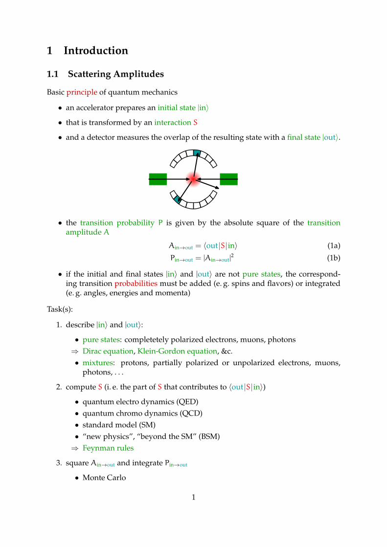
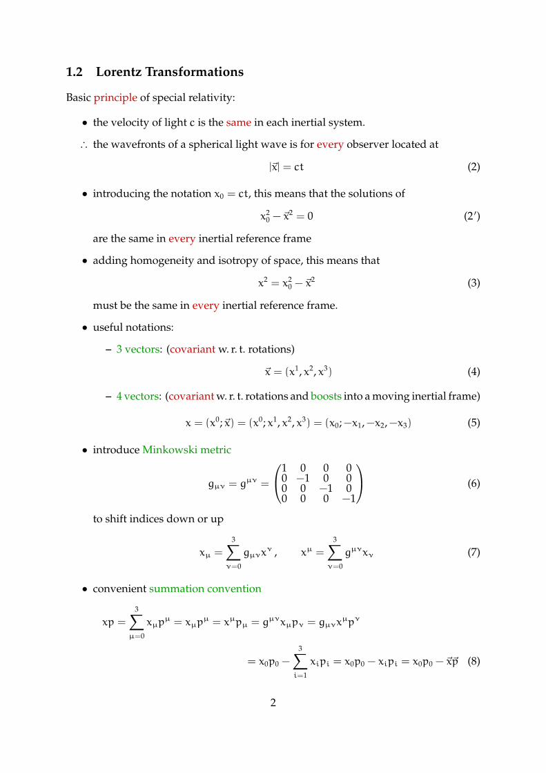
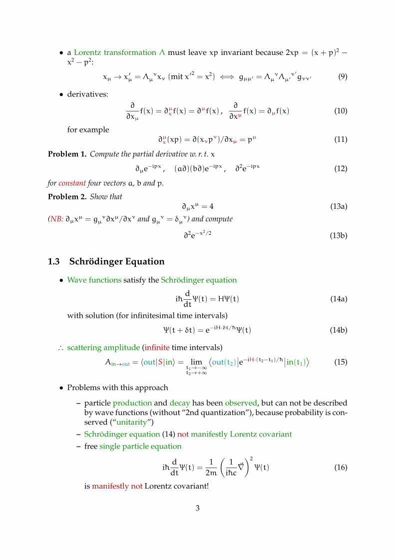
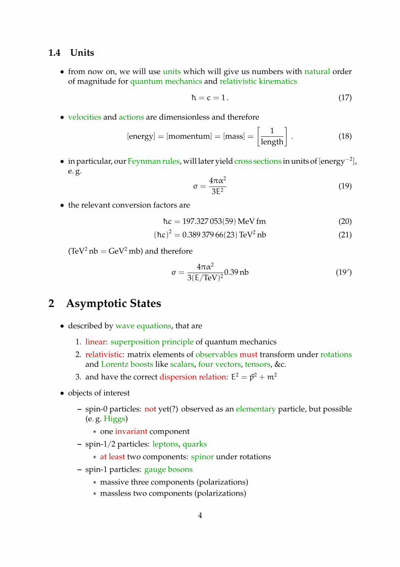
• an accelerator prepares an initial state |in〉
• that is transformed by an interaction S
• and a detector measures the overlap of the resulting state with a final state |out〉.
• the transition probability P is given by the absolute square of the transitionamplitude A
Ain→out = 〈out S in〉 (1a)
Pin→out = |Ain→out|2 (1b)
• if the initial and final states |in〉 and |out〉 are not pure states, the correspond-ing transition probabilities must be added (e. g. spins and flavors) or integrated(e. g. angles, energies and momenta)
Task(s):
1. describe |in〉 and |out〉:
• pure states: completetely polarized electrons, muons, photons⇒ Dirac equation, Klein-Gordon equation, &c.• mixtures: protons, partially polarized or unpolarized electrons, muons,
photons, . . .
2. compute S (i. e. the part of S that contributes to 〈out S in〉)
• quantum electro dynamics (QED)• quantum chromo dynamics (QCD)• standard model (SM)• “new physics”, “beyond the SM” (BSM)⇒ Feynman rules
3. square Ain→out and integrate Pin→out
• Monte Carlo
1
1.2 Lorentz Transformations
Basic principle of special relativity:
• the velocity of light c is the same in each inertial system.
∴ the wavefronts of a spherical light wave is for every observer located at
|~x| = ct (2)
• introducing the notation x0 = ct, this means that the solutions of
x20 − ~x2 = 0 (2 ′)
are the same in every inertial reference frame
• adding homogeneity and isotropy of space, this means that
x2 = x20 − ~x2 (3)
must be the same in every inertial reference frame.
• useful notations:
– 3 vectors: (covariant w. r. t. rotations)
~x = (x1, x2, x3) (4)
– 4 vectors: (covariant w. r. t. rotations and boosts into a moving inertial frame)
x = (x0;~x) = (x0; x1, x2, x3) = (x0;−x1,−x2,−x3) (5)
• introduce Minkowski metric
gµν = gµν =
1 0 0 00 −1 0 00 0 −1 00 0 0 −1
(6)
to shift indices down or up
xµ =
3∑ν=0
gµνxν , xµ =
3∑ν=0
gµνxν (7)
• convenient summation convention
xp =
3∑µ=0
xµpµ = xµp
µ = xµpµ = gµνxµpν = gµνxµpν
= x0p0 −
3∑i=1
xipi = x0p0 − xipi = x0p0 − ~x~p (8)
2
• a Lorentz transformation Λ must leave xp invariant because 2xp = (x + p)2 −x2 − p2:
xµ → x ′µ = Λ νµ xν (mit x ′2 = x2) ⇐⇒ gµµ ′ = Λ
νµ Λ
ν ′
µ ′ gνν ′ (9)
• derivatives:∂
∂xµf(x) = ∂µxf(x) = ∂
µf(x) ,∂
∂xµf(x) = ∂µf(x) (10)
for example∂µx(xp) = ∂(xνp
ν)/∂xµ = pµ (11)
Problem 1. Compute the partial derivative w. r. t. x
∂µe−ipx , (a∂)(b∂)e−ipx , ∂2e−ipx (12)
for constant four vectors a, b and p.
Problem 2. Show that∂µx
µ = 4 (13a)
(NB: ∂µxµ = g νµ ∂x
µ/∂xν and g νµ = δ ν
µ ) and compute
∂2e−x2/2 (13b)
1.3 Schrödinger Equation
• Wave functions satisfy the Schrödinger equation
i hddtΨ(t) = HΨ(t) (14a)
with solution (for infinitesimal time intervals)
Ψ(t+ δt) = e−iH·δt/ hΨ(t) (14b)
∴ scattering amplitude (infinite time intervals)
Ain→out = 〈out S in〉 = limt1→−∞t2→+∞
⟨out(t2) e−iH·(t2−t1)/ h in(t1)
⟩(15)
• Problems with this approach
– particle production and decay has been observed, but can not be describedby wave functions (without “2nd quantization”), because probability is con-served (“unitarity”)
– Schrödinger equation (14) not manifestly Lorentz covariant– free single particle equation
i hddtΨ(t) =
12m
(1
i hc~∇)2
Ψ(t) (16)
is manifestly not Lorentz covariant!
3
1.4 Units
• from now on, we will use units which will give us numbers with natural orderof magnitude for quantum mechanics and relativistic kinematics
h = c = 1 . (17)
• velocities and actions are dimensionless and therefore
[energy] = [momentum] = [mass] =[
1length
]. (18)
• in particular, our Feynman rules, will later yield cross sections in units of [energy−2],e. g.
σ =4πα2
3E2 (19)
• the relevant conversion factors are
hc = 197.327 053(59)MeV fm (20)
( hc)2= 0.389 379 66(23)TeV2 nb (21)
(TeV2 nb = GeV2 mb) and therefore
σ =4πα2
3(E/TeV)2 0.39 nb (19 ′)
2 Asymptotic States
• described by wave equations, that are
1. linear: superposition principle of quantum mechanics
2. relativistic: matrix elements of observables must transform under rotationsand Lorentz boosts like scalars, four vectors, tensors, &c.
3. and have the correct dispersion relation: E2 = ~p2 +m2
• objects of interest
– spin-0 particles: not yet(?) observed as an elementary particle, but possible(e. g. Higgs)
∗ one invariant component
– spin-1/2 particles: leptons, quarks
∗ at least two components: spinor under rotations
– spin-1 particles: gauge bosons
∗ massive three components (polarizations)∗ massless two components (polarizations)
4
2.1 Klein-Gordon Equation
(i∂0)2φ(x) =
[(−i~∂)2 +m2
]φ(x) (22)
• is obviously a covariant wave equation, because(+m2)φ(x) = 0 (23)
• fourier transform
φ(x) =
∫d4p
(2π)4 e−ipxφ(p) , i∂µφ(x) =∫
d4p
(2π)4 e−ipxpµφ(p) , etc (24)
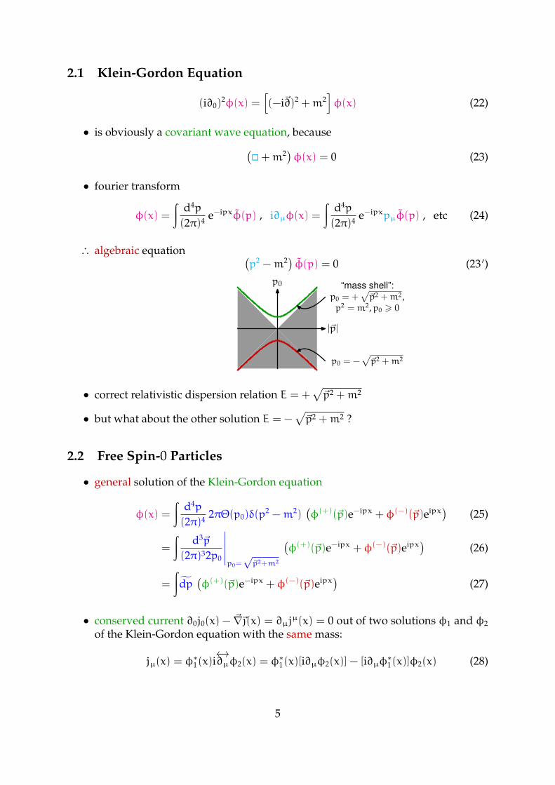
∴ algebraic equation (p2 −m2) φ(p) = 0 (23 ′)
|~p|
p0 “mass shell”:p0 = +
√~p2 +m2,
p2 = m2,p0 > 0
p0 = −√~p2 +m2
• correct relativistic dispersion relation E = +√~p2 +m2
• but what about the other solution E = −√~p2 +m2 ?
2.2 Free Spin-0 Particles
• general solution of the Klein-Gordon equation
φ(x) =
∫d4p
(2π)4 2πΘ(p0)δ(p2 −m2)
(φ(+)(~p)e−ipx + φ(−)(~p)eipx) (25)
=
∫d3~p
(2π)32p0
∣∣∣∣∣p0=√
~p2+m2
(φ(+)(~p)e−ipx + φ(−)(~p)eipx) (26)
=
∫dp(φ(+)(~p)e−ipx + φ(−)(~p)eipx) (27)
• conserved current ∂0j0(x) − ~∇~(x) = ∂µjµ(x) = 0 out of two solutions φ1 and φ2
of the Klein-Gordon equation with the same mass:
jµ(x) = φ∗1(x)i
←→∂µφ2(x) = φ
∗1(x)[i∂µφ2(x)] − [i∂µφ∗1(x)]φ2(x) (28)
5
• indeed
∂µjµ(x) = ∂µ
(φ∗1(x)[i∂µφ2(x)]
)− ∂µ
([i∂µφ∗1(x)]φ2(x)
)= i[∂µφ∗1(x)][∂µφ2(x)] + iφ∗1(x)[∂
2φ2(x)] − i[∂2φ∗1(x)]φ2(x)
−i[∂µφ∗1(x)][∂µφ2(x)] = −iφ∗1(x)m
2φ2(x) + im2φ∗1(x)φ2(x) = 0 (29)
• invariant and time independent overlap out of the conserved current
Q =
∫x0=t
d3~x j0(x) =
∫x0=t
d3~xφ∗1(x)i←→∂0φ2(x) =
∫d3~p
(2π)32p0
12p0
(φ(+)∗1 (~p)φ
(+)2 (~p) · eip0ti
←→∂0 e−ip0t + φ
(−)∗1 (−~p)φ
(+)2 (~p) · e−ip0ti
←→∂0 e−ip0t
+ φ(+)∗1 (~p)φ
(−)2 (−~p) · eip0ti
←→∂0 eip0t + φ
(−)∗1 (−~p)φ
(−)2 (−~p) · e−ip0ti
←→∂0 eip0t
)=
∫dp(φ(+)∗1 (~p)φ
(+)2 (~p) − φ
(−)∗1 (~p)φ
(−)2 (~p)
)(30)
• normalization only positive on the positive mass shell!
∴ jµ(x) must not be interpreted as a probability current!
• . . . anyway: the existence of the negative mass shell makes the energy un-bounded from below and no ground state exists!
∴ φ(x) must not be interpreted as Schrödinger wave function!
2.3 Anti Particles
Observations:
• the positive and negative mass shells of free (i. e. not interacting) particles areindependent
∴ one can simply project out the negative mass shell in this case . . .
• . . . unfortunately, all local and Lorentz invariant interactions couple positiveand negative mass shell (see below)
• . . . however, asymptotic states are assumed to be noninteracting
∴ we can at least reinterpret the negative mass shell
however:
• the amplitudeφ(+)(~p)e−ipx on the positive mass shell corresponds to the momem-tum +~p, but the amplitude φ(−)(~p)e+ipx on the negative mass shell correspondsto the reversed momemtum −~p
6
∴ the formalism is consistent, if all quantum numbers are reversed on the negativemass shell
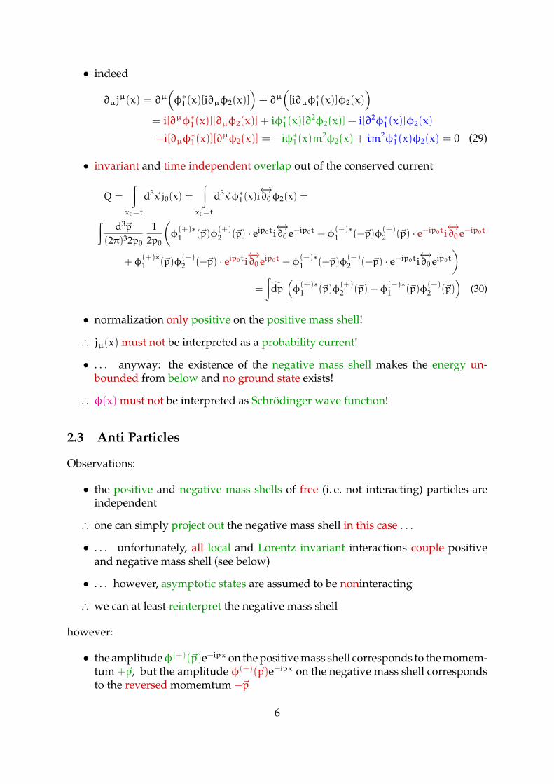
∵ in a stationary, i. e. time independent, state, the cases
Q,~p−Q,−~pQ,~p
−Q,−~p
can not be distinguished.
∴ the states on the negative mass shell describe not particles with “negative energy”,but anti particles with opposite quantum numbers instead!
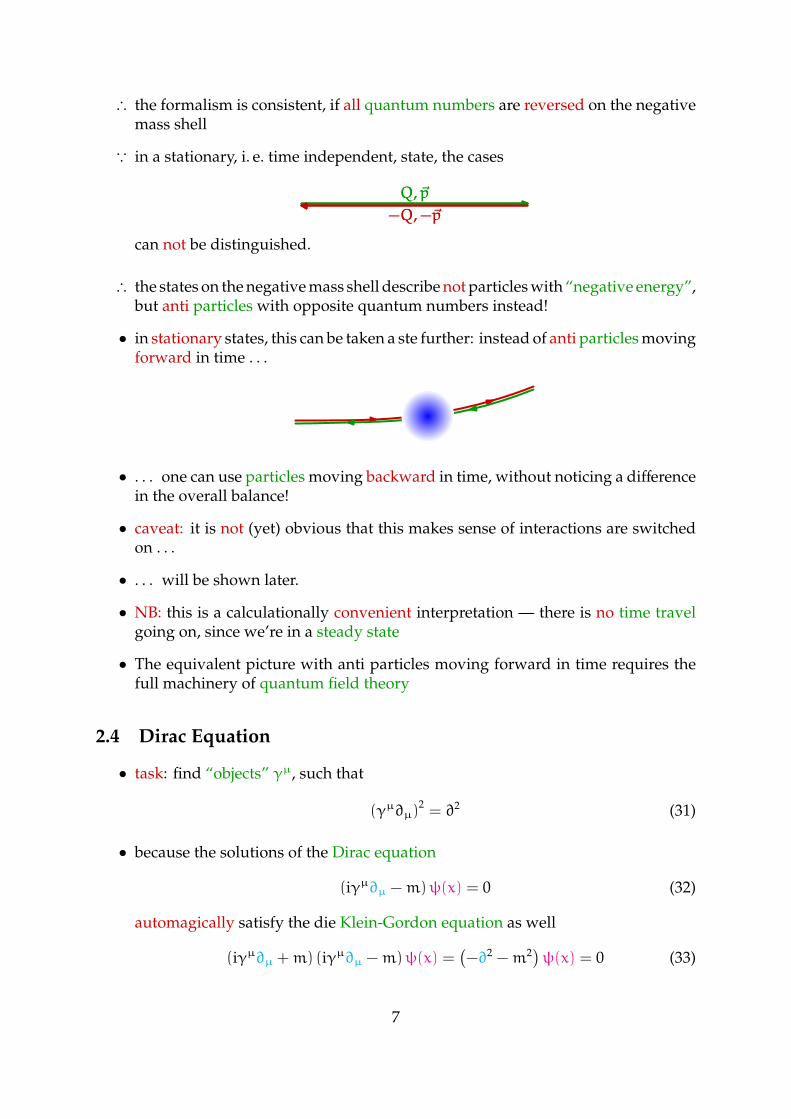
• in stationary states, this can be taken a ste further: instead of anti particles movingforward in time . . .
• . . . one can use particles moving backward in time, without noticing a differencein the overall balance!
• caveat: it is not (yet) obvious that this makes sense of interactions are switchedon . . .
• . . . will be shown later.
• NB: this is a calculationally convenient interpretation — there is no time travelgoing on, since we’re in a steady state
• The equivalent picture with anti particles moving forward in time requires thefull machinery of quantum field theory
2.4 Dirac Equation
• task: find “objects” γµ, such that
(γµ∂µ)2= ∂2 (31)
• because the solutions of the Dirac equation
(iγµ∂µ −m)ψ(x) = 0 (32)
automagically satisfy the die Klein-Gordon equation as well
(iγµ∂µ +m) (iγµ∂µ −m)ψ(x) =(−∂2 −m2)ψ(x) = 0 (33)
7
• the Dirac equation is obviously linear and its solutions satisfy the proper rela-tivistic dispersion relation.
• can we construct “objects” γµ, that satisfy (31)?
• a sufficient condition is
[γµ,γν]+ := γµγν+γνγµ = 2gµν · 1 (34)
because partial derivatives commute ∂µ∂ν = ∂ν∂µ.
• using a useful and ubiquitous notation, the Feynman slash
/a = γµaµ = γµaµ (35)
this reads equivalently [/a, /b]+ := /a/b+/b/a = 2 · ab = 2 · aµbµ
2.5 Gamma Matrices
• recall the Pauli matrices with the defining property
[σk,σl
]= σkσl − σlσk = 2i
3∑m=1
εklmσm (36a)
(σk)†
= σk (36b)
using the totally antisymmetric tensor ε
ε123 = ε231 = ε312 = 1, ε213 = ε321 = ε132 = −1 (37)
• concrete realisation
σ1 =
(0 11 0
), σ2 =
(0 −ii 0
), σ3 =
(1 00 −1
)(38)
• with
σkσl = δkl1 + i3∑
m=1
εklmσm (39)
• in particular [σk,σl
]+= 2δkl1 (40)
• Dirac realisation of the gamma (a. k. a. Dirac) matrices:
γ0 =
(1 00 −1
), γi =
(0 σi
−σi 0
)(41)
• there are (infinitely) many more realisations, but no smaller one
8
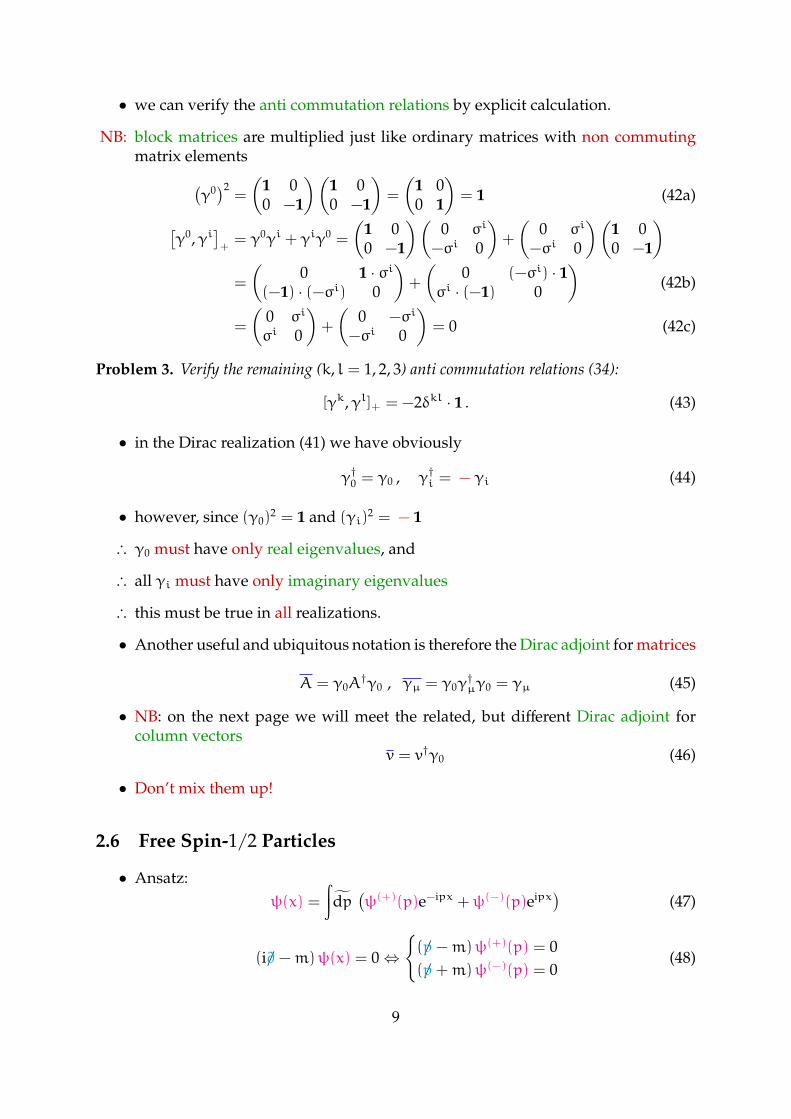
• we can verify the anti commutation relations by explicit calculation.
NB: block matrices are multiplied just like ordinary matrices with non commutingmatrix elements(
γ0)2=
(1 00 −1
)(1 00 −1
)=
(1 00 1
)= 1 (42a)
[γ0,γi
]+= γ0γi + γiγ0 =
(1 00 −1
)(0 σi
−σi 0
)+
(0 σi
−σi 0
)(1 00 −1
)=
(0 1 · σi
(−1) · (−σi) 0
)+
(0 (−σi) · 1
σi · (−1) 0
)(42b)
=
(0 σi
σi 0
)+
(0 −σi
−σi 0
)= 0 (42c)
Problem 3. Verify the remaining (k, l = 1, 2, 3) anti commutation relations (34):
[γk,γl]+ = −2δkl · 1 . (43)
• in the Dirac realization (41) we have obviously
γ†0 = γ0 , γ†i = − γi (44)
• however, since (γ0)2 = 1 and (γi)
2 = − 1
∴ γ0 must have only real eigenvalues, and
∴ all γi must have only imaginary eigenvalues
∴ this must be true in all realizations.
• Another useful and ubiquitous notation is therefore the Dirac adjoint for matrices
A = γ0A†γ0 , γµ = γ0γ
†µγ0 = γµ (45)
• NB: on the next page we will meet the related, but different Dirac adjoint forcolumn vectors
v = v†γ0 (46)
• Don’t mix them up!
2.6 Free Spin-1/2 Particles
• Ansatz:ψ(x) =
∫dp(ψ(+)(p)e−ipx +ψ(−)(p)eipx) (47)
(i/∂−m)ψ(x) = 0⇔
(/p−m)ψ(+)(p) = 0(/p+m)ψ(−)(p) = 0
(48)
9
• the adjoint solution
ψ(x) = ψ(x)†γ0 =
∫dp(ψ(+)(p)eipx + ψ(−)(p)e−ipx) (49)
satisfies
ψ(x)i←−/∂ = i∂µψ(x)γµ = i∂µψ(x)†γ0γ
µγ0γ0
= i∂µψ(x)†γµ†γ0 = (−i∂µγµψ(x))†γ0 = (−i/∂ψ(x)) = −mψ(x) (50)
∴ψ(x)
(i←−/∂ +m
)= 0 , (51)
or
ψ(+)(p) (/p−m) = 0 (52a)
ψ(−)(p) (/p+m) = 0 (52b)
• general solution of the Dirac equation
ψ(+)(p) =
2∑k=1
uk(p)bk(p) (53a)
ψ(−)(p) =
2∑k=1
vk(p)dk(p) (53b)
with four independent basis solutions u1(p), u2(p), v1(p), v2(p) satisfying
(/p−m)uk(p) = 0 (54a)(/p+m)vk(p) = 0 (54b)
and the corresponding expansion coefficients b1(p), b2(p), d1(p), d2(p).
• in the rest frame of the particle, i. e. for p = (m,~0), we have /p = mγ0 and theDirac equation simplifies to
m(γ0 − 1)uk(~0) =(
0 00 −2m · 1
)uk(~0) = 0 (55a)
m(γ0 + 1)vk(~0) =(
2m · 1 00 0
)vk(~0) = 0 (55b)
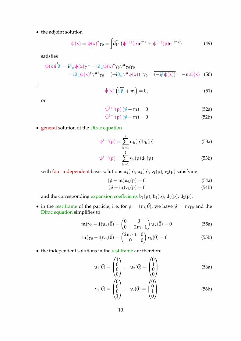
• the independent solutions in the rest frame are therefore
u1(~0) =
1000
, u2(~0) =
0100
(56a)
v1(~0) =
0001
, v2(~0) =
0010
(56b)
10
• from which we can construct solutions for arbitrary on shell momenta with p2 =m2
uk(p) =/p+m√p0 +m
uk(~0) (57a)
vk(p) =/p−m√p0 +m
vk(~0) (57b)
• since (/p+m)(/p−m) = p2−m2, these are obviously solutions of the Dirac equationfor on-shell momenta
• the motivation for the not obviously covariant normalization will be apparentafter problem 4
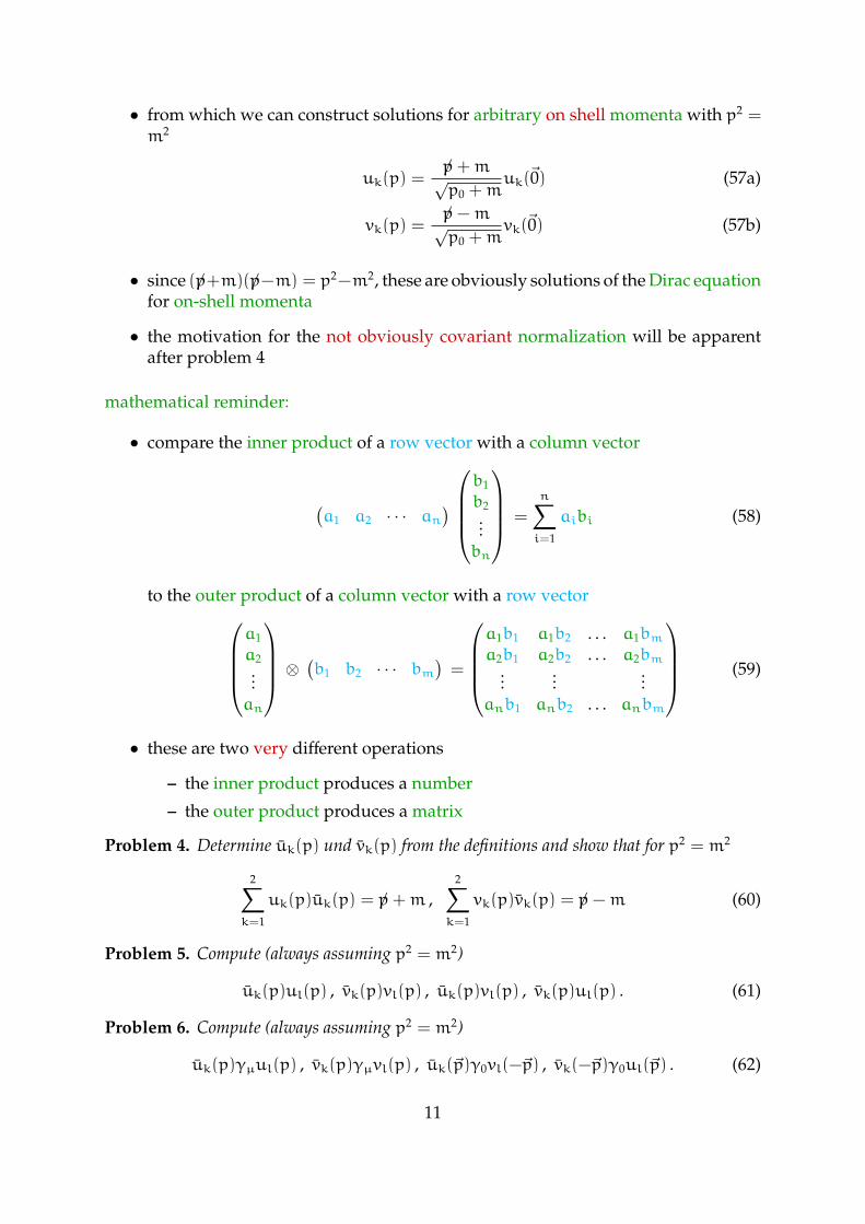
mathematical reminder:
• compare the inner product of a row vector with a column vector
(a1 a2 · · · an
)b1
b2...bn
=
n∑i=1
aibi (58)
to the outer product of a column vector with a row vectora1
a2...an
⊗ (b1 b2 · · · bm)=
a1b1 a1b2 . . . a1bma2b1 a2b2 . . . a2bm
......
...anb1 anb2 . . . anbm
(59)
• these are two very different operations
– the inner product produces a number
– the outer product produces a matrix
Problem 4. Determine uk(p) und vk(p) from the definitions and show that for p2 = m2
2∑k=1
uk(p)uk(p) = /p+m ,2∑k=1
vk(p)vk(p) = /p−m (60)
Problem 5. Compute (always assuming p2 = m2)
uk(p)ul(p) , vk(p)vl(p) , uk(p)vl(p) , vk(p)ul(p) . (61)
Problem 6. Compute (always assuming p2 = m2)
uk(p)γµul(p) , vk(p)γµvl(p) , uk(~p)γ0vl(−~p) , vk(−~p)γ0ul(~p) . (62)
11
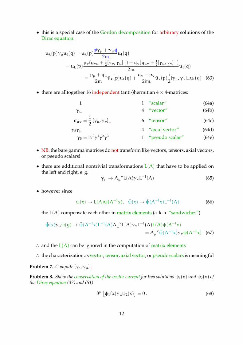
• this is a special case of the Gordon decomposition for arbitrary solutions of theDirac equation:
uk(p)γµul(q) = uk(p)/pγµ + γµ/q
2mul(q)
= uk(p)pν(gνµ +
12 [γν,γµ]−) + qν(gµν + 1
2 [γµ,γν]−)2m
ul(q)
=pµ + qµ
2muk(p)ul(q) +
qν − pν2im
uk(p)i2[γµ,γν]−ul(q) (63)
• there are alltogether 16 independent (anti-)hermitian 4× 4-matrices:
1 1 “scalar” (64a)γµ 4 “vector” (64b)
σµν =i2[γµ,γν]− 6 “tensor” (64c)
γ5γµ 4 “axial vector” (64d)
γ5 = iγ0γ1γ2γ3 1 “pseudo scalar” (64e)
• NB: the bare gamma matrices do not transform like vectors, tensors, axial vectors,or pseudo scalars!
• there are additional nontrivial transformations L(Λ) that have to be applied onthe left and right, e. g.
γµ → Λ νµ L(Λ)γνL
−1(Λ) (65)
• however since
ψ(x)→ L(Λ)ψ(Λ−1x) , ψ(x)→ ψ(Λ−1x)L−1(Λ) (66)
the L(Λ) compensate each other in matrix elements (a. k. a. “sandwiches”)
ψ(x)γµψ(y)→ ψ(Λ−1x)L−1(Λ)Λ νµ L(Λ)γνL
−1(Λ)L(Λ)ψ(Λ−1x)
= Λ νµ ψ(Λ
−1x)γνψ(Λ−1x) (67)
∴ and the L(Λ) can be ignored in the computation of matrix elements
∴ the characterization as vector, tensor, axial vector, or pseudo scalars is meaningful
Problem 7. Compute [γ5,γµ]+
Problem 8. Show the conservation of the vector current for two solutions ψ1(x) und ψ2(x) ofthe Dirac equation (32) and (51)
∂µ[ψ1(x)γµψ2(x)
]= 0 . (68)
12
• invariant overlap from conserved current:
Q =
∫x0=t
d3~x j0(x) =
∫x0=t
d3~x ψ1(x)γ0ψ2(x) =
∫x0=t
d3~xψ†1(x)ψ2(x)
=
∫d3~p
(2π)32p0
12p0
(ψ
(+)†1 (~p)ψ
(+)2 (~p) +ψ
(−)†1 (−~p)ψ
(+)2 (~p) · e−2ip0t
+ψ(+)†1 (~p)ψ
(−)2 (−~p) · e2ip0t +ψ
(−)†1 (−~p)ψ
(−)2 (−~p)
)=
∫d3~p
(2π)32p0
2∑k=1
(b†1,k(p)b2,k(~p) + d
†1,k(p)d2,k(~p)
)(69)
∴ normalization positive everywhere!
Problem 9. Show the Partial Conservation of the Axial Current (PCAC) for solutions ψ1(x)und ψ2(x) of the Dirac equation
∂µ[ψ1(x)γµγ5ψ2(x)
]= 2imψ1(x)γ5ψ2(x) . (70)
Problem 10. Compute σkl = i2 [γk,γl]− for k, l = 1, 2, 3 in the Dirac realization of the
Gamma matrices.
∴ the matrices σ23,σ31,σ12 can take over the rôle of the Pauli matrices σ1,σ2,σ3
and distinguish spin up from spin down in the rest frame
12σ12u1(~0) = +
12u1(~0) ,
12σ12u2(~0) = −
12u2(~0) (71a)
12σ12v1(~0) = +
12v1(~0) ,
12σ12v2(~0) = −
12v2(~0) (71b)
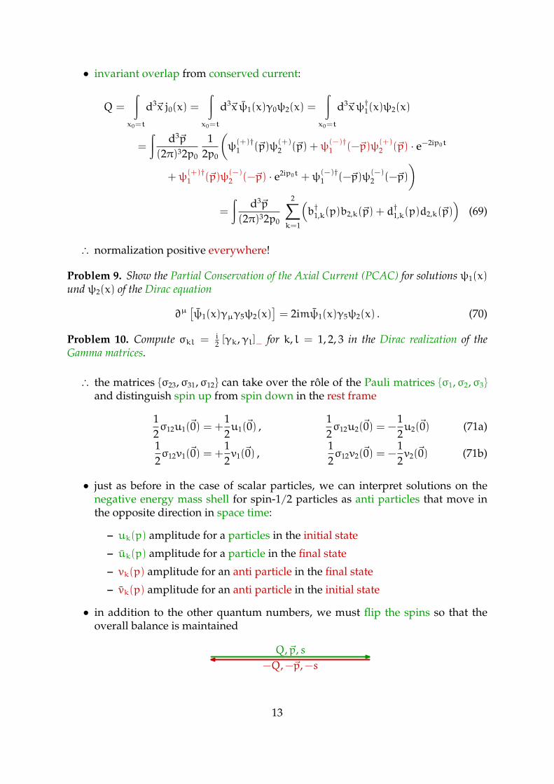
• just as before in the case of scalar particles, we can interpret solutions on thenegative energy mass shell for spin-1/2 particles as anti particles that move inthe opposite direction in space time:
– uk(p) amplitude for a particles in the initial state
– uk(p) amplitude for a particle in the final state
– vk(p) amplitude for an anti particle in the final state
– vk(p) amplitude for an anti particle in the initial state
• in addition to the other quantum numbers, we must flip the spins so that theoverall balance is maintained
Q,~p, s−Q,−~p,−s
13
2.7 Free Spin-1 Particles
• combine ~E and ~B into field strength tensor
Fµν = ∂µAν − ∂νAµ =
0 −E1 −E2 −E3
E1 0 −B3 B2
E2 B3 0 −B1
E3 −B2 B1 0
(72)
• manifestly covariant Maxwell equations
∂µFµν = jν , εµνρσ∂νFρσ = 0 (73)
• current jµ necessarily conserved: ∂µjµ = 0
• equation of motion for the vector potential Aµ
(gµν∂2 − ∂µ∂ν)Aν = jµ (73 ′)
• gauge invariance: Fµν does not change, if
Aµ(x)→ Aµ(x) − ∂µω(x) (74)
• with special gauge condition ∂µAµ = 0: ∂2Aµ = jµ
• more, but not most, general case
(gµν∂2 − (1 − ξ)∂µ∂ν)Aν = jµ (75)
• explicit mass term∂µFµν +M
2Aν = jν (76)
or(gµν(∂2 +M2) − ∂µ∂ν)Aν = jµ (76 ′)
• contraction with ∂µM2∂νAν = 0 (77)
• massless vector bososns have two degrees of freedom, massive ones three
• polarization vectors for massless vector bosons with momentum k = (k0; 0, 0, k0)
ε± = ε∗∓ =1√2(0; 1,±i, 0) (78)
• properties
εµλε∗λ ′,µ = −δλλ ′ (79a)
εµλkµ = 0 (79b)
and with c = (1; 0, 0,−1)∑λ=−1,+1
εµλεν,∗λ = −gµν +
cµkν + cνkµck
(80)
• polarization vectors for massive vector bosons with momentum
14
k = (k0; |~k| sin θ cosφ, |~k| sin θ sinφ, |~k| cos θ):
ε± = ε∗∓ =e∓iφ√
2(0; cos θ cosφ∓ i sinφ, cos θ sinφ± i cosφ,− sin θ) (81a)
ε0 =k0
M(|~k|/k0; sin θ cosφ, sin θ sinφ, cos θ) = ε∗0 (81b)
• properties (79) and ∑λ=−1,0,+1
εµλεν,∗λ = −gµν +
kµkν
M2 (82)
3 Interactions
3.1 Propagators
• Photons far from all electrical charges satisfy
∂2A(0)µ (x) = 0 (83)
and we have already seen the solutions.
• In the presence of electrical charges, the photons couple to the electromagneticcurrent
∂2Aµ(x) = jµ(x) = −eψ(x)γµψ(x) + . . . (84)
and the solutions turn out to be more complicated.
• Assumption: there is a “function” D, that solves
(∂2 +m2)D(x,m) = −δ4(x) (85)
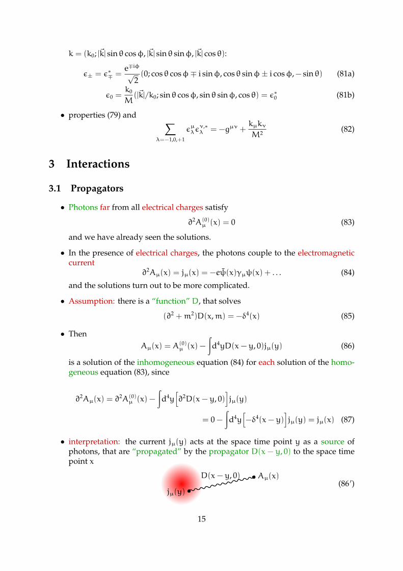
• ThenAµ(x) = A
(0)µ (x) −
∫d4yD(x− y, 0)jµ(y) (86)
is a solution of the inhomogeneous equation (84) for each solution of the homo-geneous equation (83), since
∂2Aµ(x) = ∂2A(0)µ (x) −
∫d4y[∂2D(x− y, 0)
]jµ(y)
= 0 −
∫d4y[−δ4(x− y)
]jµ(y) = jµ(x) (87)
• interpretation: the current jµ(y) acts at the space time point y as a source ofphotons, that are “propagated” by the propagator D(x − y, 0) to the space timepoint x
D(x− y, 0) Aµ(x)
jµ(y)(86 ′)
15
• NB: retardation is built in in (86), because we integrate over the four dimensionalspace time and not over the three dimensional space at a given instant.
Problem 11. Show thatS(x,m) = (i/∂+m)D(x,m) (88)
is the Feynman propagator S for Dirac particles of massm, i. e. that
(i/∂−m)S(x,m) = δ4(x)
if (∂2 +m2)D(x,m) = −δ4(x), as in (85) above.
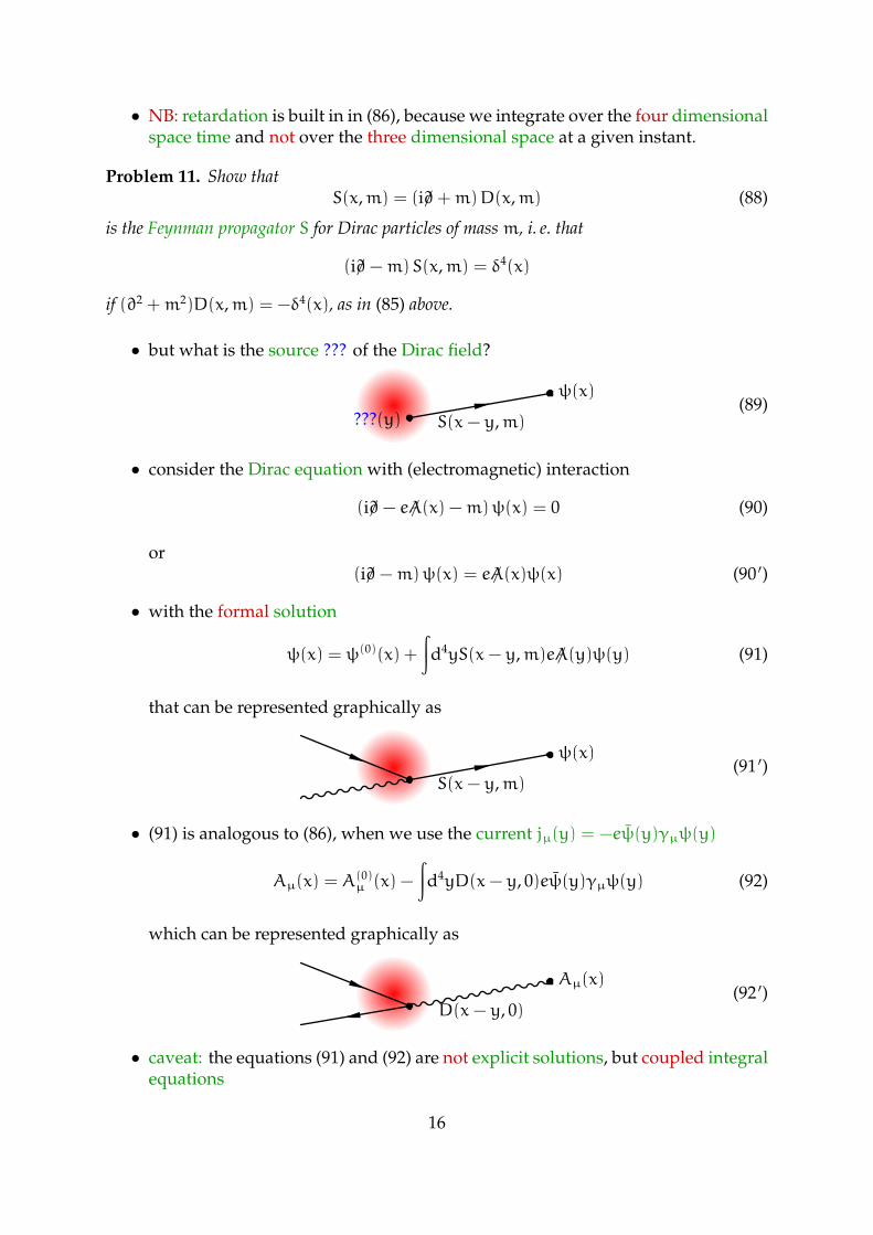
• but what is the source ??? of the Dirac field?
S(x− y,m)
ψ(x)
???(y)(89)
• consider the Dirac equation with (electromagnetic) interaction
(i/∂− e/A(x) −m)ψ(x) = 0 (90)
or(i/∂−m)ψ(x) = e/A(x)ψ(x) (90 ′)
• with the formal solution
ψ(x) = ψ(0)(x) +
∫d4yS(x− y,m)e/A(y)ψ(y) (91)
that can be represented graphically as
S(x− y,m)
ψ(x)(91 ′)
• (91) is analogous to (86), when we use the current jµ(y) = −eψ(y)γµψ(y)
Aµ(x) = A(0)µ (x) −
∫d4yD(x− y, 0)eψ(y)γµψ(y) (92)
which can be represented graphically as
D(x− y, 0)
Aµ(x)(92 ′)
• caveat: the equations (91) and (92) are not explicit solutions, but coupled integralequations
16
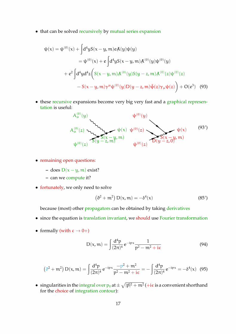
• that can be solved recursively by mutual series expansion
ψ(x) = ψ(0)(x) +
∫d4yS(x− y,m)e/A(y)ψ(y)
= ψ(0)(x) + e
∫d4yS(x− y,m)/A(0)(y)ψ(0)(y)
+ e2∫
d4yd4z
(S(x− y,m)/A(0)(y)S(y− z,m)/A(0)(z)ψ(0)(z)
− S(x− y,m)γµψ(0)(y)D(y− z,m)ψ(z)γµψ(z)
)+O(e3) (93)
• these recursive expansions become very big very fast and a graphical represen-tation is useful:
S(x− y,m)S(y− z,m)
ψ(x)
ψ(0)(z)
A(0)µ (z)
A(0)µ (y)
S(x− y,m)D(y− z, 0)
ψ(x)
ψ(0)(z)
ψ(0)(z)
ψ(0)(y)
(93 ′)
• remaining open questions:
– does D(x− y,m) exist?
– can we compute it?
• fortunately, we only need to solve(∂2 +m2)D(x,m) = −δ4(x) (85 ′)
because (most) other propagators can be obtained by taking derivatives
• since the equation is translation invariant, we should use Fourier transformation
• formally (with ε→ 0+)
D(x,m) =
∫d4p
(2π)4 e−ipx 1p2 −m2 + iε
(94)
(∂2 +m2)D(x,m) =
∫d4p
(2π)4 e−ipx −p2 +m2
p2 −m2 + iε= −
∫d4p
(2π)4 e−ipx = −δ4(x) (95)
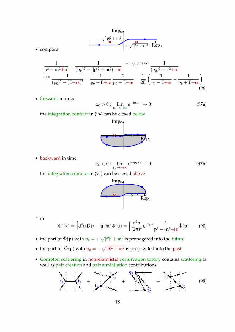
• singularities in the integral overp0 at±√
|~p|2 +m2 (+iε is a convenient shorthandfor the choice of integration contour):
17
Imp0
Rep0
−√|~p|2 +m2
+√|~p|2 +m2
• compare
1p2 −m2+iε
=1
(p0)2 − (|~p|2 +m2)+iεE=+√
|~p|2+m2
=1
(p0)2 − E2+iεE>0=
1(p0)2 − (E−iε)2 =
1p0 − E+iε
1p0 + E−iε
=1
2E
(1
p0 − E+iε−
1p0 + E−iε
)(96)
• forward in time:x0 > 0 : lim
p0→−i∞ e−ip0x0 → 0 (97a)
the integration contour in (94) can be closed below
Imp0
Rep0
• backward in time:x0 < 0 : lim
p0→+i∞ e−ip0x0 → 0 (97b)
the integration contour in (94) can be closed above
Imp0
Rep0
∴ in
Φ ′(x) =
∫d4yD(x− y,m)Φ(y) =
∫d4p
(2π)4 e−ipx 1p2 −m2+iε
Φ(p) (98)
• the part of Φ(p) with p0 = +√|~p|2 +m2 is propagated into the future
• the part of Φ(p) with p0 = −√
|~p|2 +m2 is propagated into the past
• Compton scattering in nonrelativistic perturbation theory contains scattering aswell as pair creation and pair annihilation contributions:
t1 t2 +t1
t2+
t2
t1
+t2
t1(99)
18
∵ intermediate states violate energy conservation and vertices can have space likedistances
∴ temporal order of t1 and t2 depends in general on the reference frame, i. e. isundefined
• Feynman’s brilliant (re-)interpretation:
– particles with p0 = +√|~p|2 +m2 are propagated into the future
– anti particles with p0 = −√|~p|2 +m2 and opposite charges are propagated
into past
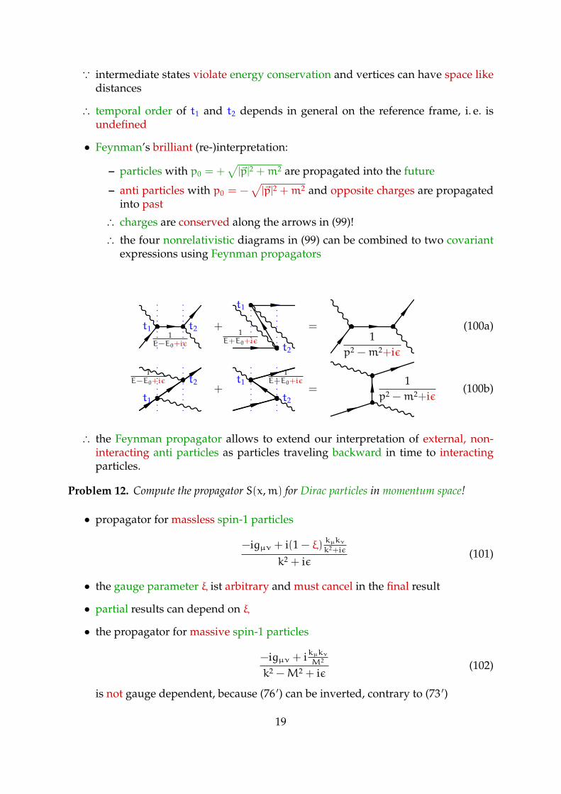
∴ charges are conserved along the arrows in (99)!
∴ the four nonrelativistic diagrams in (99) can be combined to two covariantexpressions using Feynman propagators
1E−E0+iε
t1 t2 +1
E+E0+iεt2
t1
=1
p2 −m2+iε
(100a)
1E−E0+iε
t1
t2+
1E+E0+iε
t2
t1=
1p2 −m2+iε
(100b)
∴ the Feynman propagator allows to extend our interpretation of external, non-interacting anti particles as particles traveling backward in time to interactingparticles.
Problem 12. Compute the propagator S(x,m) for Dirac particles in momentum space!
• propagator for massless spin-1 particles
−igµν + i(1 − ξ)kµkνk2+iε
k2 + iε(101)
• the gauge parameter ξ ist arbitrary and must cancel in the final result
• partial results can depend on ξ
• the propagator for massive spin-1 particles
−igµν + ikµkνM2
k2 −M2 + iε(102)
is not gauge dependent, because (76 ′) can be inverted, contrary to (73 ′)
19
• NB: this is not what happens in the standard model, where the mass comessolely from the coupling to the Higgs sector and a gauge freedom remains.However (102) is in lowest order equivalent to the Higgs mechanism in unitaritygauge
• NB: propagators and external states are universal and models differ only in theparticle content and interaction vertices!
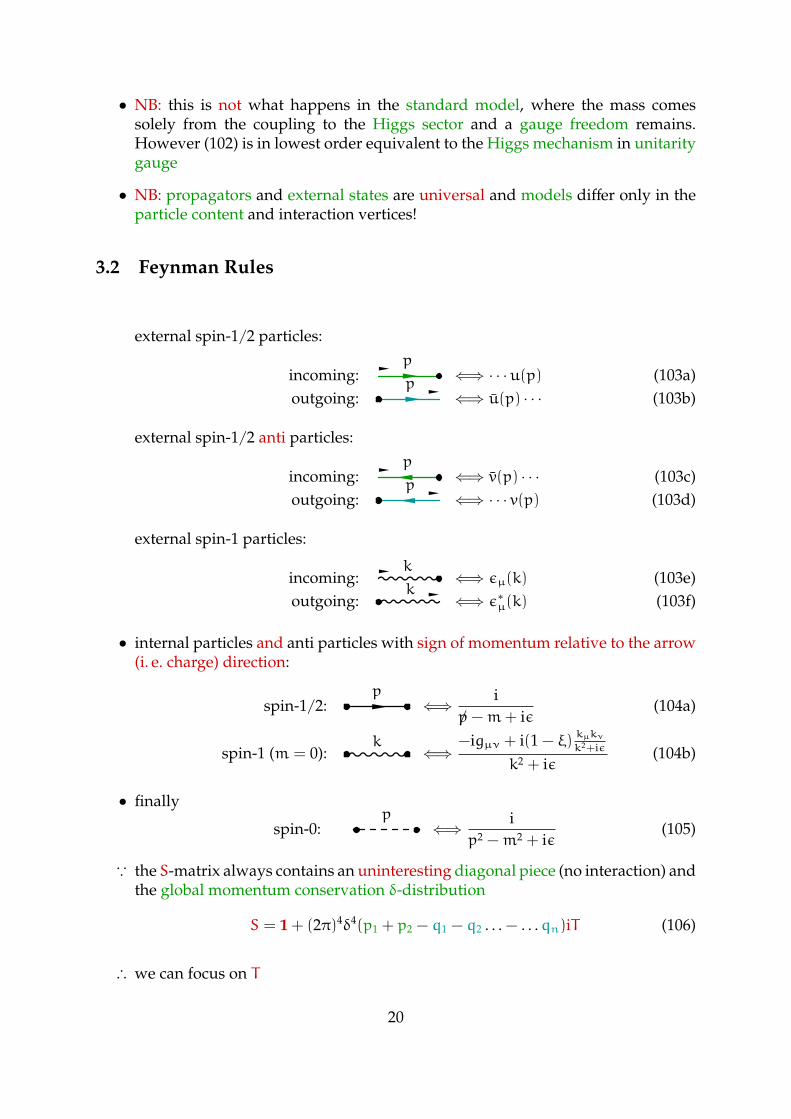
3.2 Feynman Rules
external spin-1/2 particles:
incoming:p
⇐⇒ · · ·u(p) (103a)outgoing:
p⇐⇒ u(p) · · · (103b)
external spin-1/2 anti particles:
incoming:p
⇐⇒ v(p) · · · (103c)outgoing:
p⇐⇒ · · · v(p) (103d)
external spin-1 particles:
incoming:k
⇐⇒ εµ(k) (103e)outgoing:
k⇐⇒ ε∗µ(k) (103f)
• internal particles and anti particles with sign of momentum relative to the arrow(i. e. charge) direction:
spin-1/2:p
⇐⇒ i/p−m+ iε
(104a)
spin-1 (m = 0):k
⇐⇒−igµν + i(1 − ξ)
kµkνk2+iε
k2 + iε(104b)
• finally
spin-0:p
⇐⇒ ip2 −m2 + iε
(105)
∵ the S-matrix always contains an uninteresting diagonal piece (no interaction) andthe global momentum conservation δ-distribution
S = 1 + (2π)4δ4(p1 + p2 − q1 − q2 . . . − . . .qn)iT (106)
∴ we can focus on T
20
• the following Feynman rules produce an expression for iT :
1. draw all diagrams using propagators and interaction vertices that connectthe initial state with the final state
2. assign momenta and external wave functions accordingly3. use momentum conservation at each vertex to fix the momenta of the internal
lines4. follow each connected fermion line against the direction of the arrows and
collect wave functions, propagators and vertices along the way5. complete iT with the remaining wave functions, propagators and vertices6. add all diagrams with the relative signs such that that sum is anti symmetric
under the exchange of identical external (anti-)fermions (and symmetric forbosons)
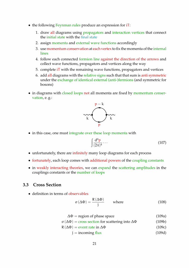
• in diagrams with closed loops not all momenta are fixed by momentum conser-vation, e. g.:
k
p
k
p− k
• in this case, one must integrate over these loop momenta with∫d4p
(2π)4 · · · (107)
• unfortunately, there are infinitely many loop diagrams for each process
• fortunately, each loop comes with additional powers of the coupling constants
• in weakly interacting theories, we can expand the scattering amplitudes in thecouplings constants or the number of loops
3.3 Cross Section
• definition in terms of observables
σ (∆Φ) =R (∆Φ)
jwhere (108)
∆Φ = region of phase space (109a)σ (∆Φ) = cross section for scattering into ∆Φ (109b)R (∆Φ) = event rate in ∆Φ (109c)
j = incoming flux (109d)
21
• for fixed target experiments, the incoming flux j is just the number of incomingparticles per time and area
• differential cross section
σ (∆Φ) =
∫∆Φ
dσdΦ
(Φ)dΦ (110)
with phase space element dΦ, e. g. dΩ = sin θdθdφ for 2→ 2 processes
• the differential cross section can be computed from the scattering amplitude Tand the (a. k. a. “Fermi’s golden rule”)
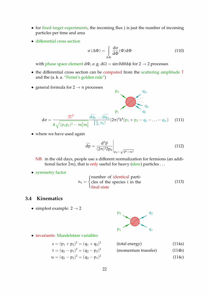
• general formula for 2→ n processes
p1
p2
q1
q2
qn
dσ =|T |
2
4√
(p1p2)2 −m21m
22
dq1 . . . dqn∏i ni!
(2π)4δ4(p1 + p2 − q1 − . . . − qn) (111)
• where we have used again
dp =d3~p
(2π)32p0
∣∣∣∣∣p0=√
~p2+m2
(112)
NB: in the old days, people use a different normalization for fermions (an addi-tional factor 2m), that is only useful for heavy (slow) particles . . .
• symmetry factor
ni =
number of identical parti-cles of the species i in thefinal state
(113)
3.4 Kinematics
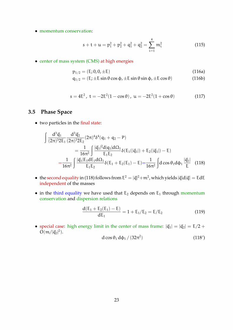
• simplest example: 2→ 2
p1
p2
q1
q2
• invariants: Mandelstam variables
s = (p1 + p2)2 = (q1 + q2)
2 (total energy) (114a)
t = (q1 − p1)2 = (q2 − p2)
2 (momentum transfer) (114b)
u = (q1 − p2)2 = (q2 − p1)
2 (114c)
22
• momentum conservation:
s+ t+ u = p21 + p
22 + q
21 + q
22 =
4∑i=1
m2i (115)
• center of mass system (CMS) at high energies
p1/2 = (E; 0, 0,±E) (116a)q1/2 = (E;±E sin θ cosφ,±E sin θ sinφ,±E cos θ) (116b)
s = 4E2 , t = −2E2(1 − cos θ) , u = −2E2(1 + cos θ) (117)
3.5 Phase Space
• two particles in the final state:∫d3~q1
(2π)32E1
d3~q2
(2π)32E2(2π)4δ4(q1 + q2 − P)
=1
16π2
∫|~q1|
2d|q1|dΩ1
E1E2δ(E1(|~q1|) + E2(|~q1|) − E)
=1
16π2
∫|~q1|E1dE1dΩ1
E1E2δ(E1 + E2(E1) − E)=
116π2
∫d cos θ1dφ1
|~q1|
E(118)
• the second equality in (118) follows fromE2 = |~q|2+m2, which yields |~q|d|~q| = EdEindependent of the masses
• in the third equality we have used that E2 depends on E1 through momentumconservation and dispersion relations
d(E1 + E2(E1) − E)
dE1= 1 + E1/E2 = E/E2 (119)
• special case: high energy limit in the center of mass frame: |~q1| = |~q2| = E/2 +O(m/|~q2|
2).d cos θ1 dφ1 / (32π2) (118 ′)
23
4 QED
• Quantum Electro Dynamics: interacting electrons, positrons and photons (andother charged particles)
• single interaction vertex for fermions:
f
f
k,µ
p
p ′
= iQfeγµ (120)
with the electrical charge Qf of the particle, e. g. Qe = −1 for electrons
• charged bosons require an additional (“sea gull”) vertex
s
s
k,µ
p
p ′
= iQse(pµ + p′µ),
k,µk ′,ν
= 2iQ2se
2gµν (121)
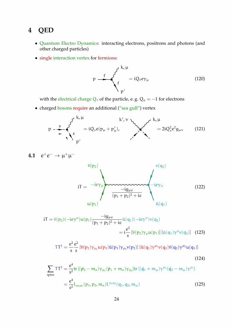
4.1 e+e− → µ+µ−
iT = −igρσ(p1 + p2)2 + iε
u(p1)
v(p2)
u(q1)
v(q2)
−ieγρ −ieγσ (122)
iT = v(p2)(−ieγρ)u(p1)−igρσ
(p1 + p2)2 + iεu(q1)(−ieγσ)v(q2)
= ie2
s[v(p2)γρu(p1)] [u(q1)γ
ρv(q2)] (123)
TT † =e2
s
e2
s[v(p2)γρ1u(p1)u(p1)γρ2v(p2)] [u(q1)γ
ρ1v(q2)v(q2)γρ2u(q1)]
(124)∑spins
TT † =e4
s2 tr [(/p2 −me)γρ1(/p1 +me)γρ2 ]tr [(/q1 +mµ)γρ1(/q2 −mµ)γ
ρ2 ]
=e4
s2Lρ2ρ1(p1,p2,me)Lρ1ρ2(q1,q2,mµ) (125)
24
4.2 Trace Techniques
• consider a matrix element
u(p)Γu(q) =
4∑k,l=1
uk(p)Γklul(q) =
4∑k,l=1
Γklul(q)uk(p) (126)
• using the tensor product
u(q)⊗ u(p) =
u1(q)u1(p) · · · u1(q)u4(p)... . . . ...
u4(q)u1(p) · · · u4(q)u4(p)
(127)
we can write
u(p)Γu(q) =
4∑k,l=1
Γkl[u(q)⊗ u(p)]lk =
4∑k=1
(Γ [u(q)⊗ u(p)])kk (128)
• using the trace of a matrix
tr(A) =4∑k=1
Akk (129)
we can express a matrix element equivalently as a trace
u(p)Γu(p) = tr(Γ [u(p)⊗ u(p)]) (130)
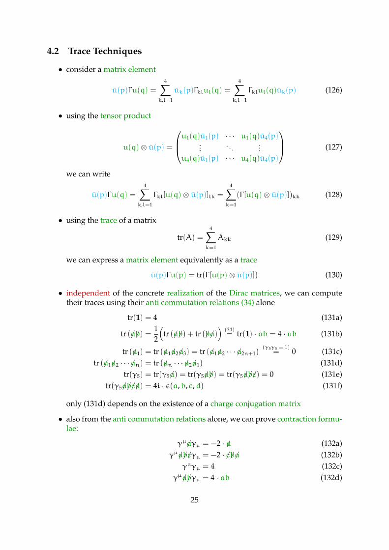
• independent of the concrete realization of the Dirac matrices, we can computetheir traces using their anti commutation relations (34) alone
tr(1) = 4 (131a)
tr (/a/b) =12
(tr (/a/b) + tr (/b/a)
)(34)= tr(1) · ab = 4 · ab (131b)
tr (/a1) = tr (/a1/a2/a3) = tr (/a1/a2 · · · /a2n+1)(γ5γ5 = 1)
= 0 (131c)tr (/a1/a2 · · · /an) = tr (/an · · · /a2/a1) (131d)
tr(γ5) = tr(γ5/a) = tr(γ5/a/b) = tr(γ5/a/b/c) = 0 (131e)tr(γ5/a/b/c/d) = 4i · ε(a,b, c,d) (131f)
only (131d) depends on the existence of a charge conjugation matrix
• also from the anti commutation relations alone, we can prove contraction formu-lae:
γµ/aγµ = −2 · /a (132a)γµ/a/b/cγµ = −2 · /c/b/a (132b)
γµγµ = 4 (132c)γµ/a/bγµ = 4 · ab (132d)
25
• it’s instructive to prove at least one of the trace theorems yourselves, because ithelps to memorize the result.
Problem 13. Computetr (/a/b/c/d) (133)
using the cyclic invariance of the trace
tr(ABC) = tr(BCA) (134)
and subsequently the anti commutation relations (34).
Problem 14. Compute the trace Lµν(p,q,m) = tr [(/p+m)γµ(/q−m)γν].
Problem 15. Compute Lρ2ρ1(p1,p2, 0)Lρ1ρ2(q1,q2, 0) as a function of the Mandelstam vari-ables in the high energy limit s,−t,−u m2
i.
4.3 Cross Section
Problem 16. Compute the differential cross section
dσdΩ
(cos θ,ECM) (135)
for e+e− → µ+µ− in the region s,−t,−u m2e.
Problem 17. Compute the integrated cross section
σ(ECM) (136)
for e+e− → µ+µ− in the region s m2e.
4.4 FORM
• very efficient computation using programs for symbolic manipulation, e. g. FORM.
• declare variables
1: vector p1, p2, q1, q2;2: symbol s, t, u, me, mq;3: indices rho1, rho2;
• expressions
4: local [TT*] =5: (g_(1, p2) - me*g_(1)) * g_(1, rho1)6: * (g_(1, p1) + me*g_(1)) * g_(1, rho2)7: * (g_(2, q1) + mq*g_(2)) * g_(2, rho1)8: * (g_(2, q2) - mq*g_(2)) * g_(2, rho2);
26
• traces
9: trace4, 1;10: trace4, 2;11: print;12: .sort;
• reduction to Mandelstam variables (114)
s = (p1 + p2)2 = 2m2
e + 2p1p2 (137a)
t = (q2 − p1)2 = m2
q +m2e − 2q2p1 (137b)
etc.
13: id p1.p2 = 1/2 * (s - 2*me^2);14: id q1.q2 = 1/2 * (s - 2*mq^2);15: id p1.q1 = - 1/2 * (t - me^2 - mq^2);16: id p2.q2 = - 1/2 * (t - me^2 - mq^2);17: id p1.q2 = - 1/2 * (u - me^2 - mq^2);18: id p2.q1 = - 1/2 * (u - me^2 - mq^2);
• human intelligence (i. e. experience, cf. (211)): the result can be written mostcompactly as a function of t und u:
19: id s = - u - t + 2*me^2 + 2*mq^2;20: bracket me, mq;21: print;22: .sort;
running the program:
ohl@thopad2:~fdfp$ form mumu.frm
FORM by J.Vermaseren,version 3.3(Mar 28 2009) Run at: Thu Jul 7 18:37:42 2011[TT*] =64*me^2*mq^2 + 32*p1.p2*mq^2 + 32*p1.q1*p2.q2 + 32*p1.q2*p2.q1 + 32*q1.q2*me^2;
[TT*] =+ mq^2 * ( - 32*u - 32*t )+ mq^4 * ( 48 )+ me^2 * ( - 32*u - 32*t )+ me^2*mq^2 * ( 96 )+ me^4 * ( 48 )+ 8*u^2 + 8*t^2;
0.00 sec out of 0.00 sec
27
4.5 Bhabha Scattering
Problem 18. Draw all Feynman diagrams for e+e− → e+e− (“Bhabha scattering”)
• do we need to add or subtract the diagrams?
• more general: what’s the relative phase of the diagrams?
TT † = (Tt − Ts)(Tt − Ts)† = TtTt
† − TtTs† − TsTt
† + TsTs† (138)
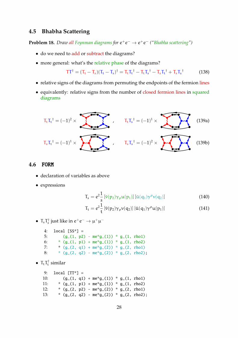
• relative signs of the diagrams from permuting the endpoints of the fermion lines
• equivalently: relative signs from the number of closed fermion lines in squareddiagrams
TtTt† = (−1)2 × , TtTs
† = (−1)1 × (139a)
TsTt† = (−1)1 × , TsTs
† = (−1)2 × (139b)
4.6 FORM
• declaration of variables as above
• expressions
Ts = e2 1s[v(p2)γρu(p1)] [u(q1)γ
ρv(q2)] (140)
Tt = e2 1t[v(p2)γρv(q2)] [u(q1)γ
ρu(p1)] (141)
• TsT†s just like in e+e− → µ+µ−
4: local [SS*] =5: (g_(1, p2) - me*g_(1)) * g_(1, rho1)6: * (g_(1, p1) + me*g_(1)) * g_(1, rho2)7: * (g_(2, q1) + me*g_(2)) * g_(2, rho1)8: * (g_(2, q2) - me*g_(2)) * g_(2, rho2);
• TtT†t similar
9: local [TT*] =10: (g_(1, q1) + me*g_(1)) * g_(1, rho1)11: * (g_(1, p1) + me*g_(1)) * g_(1, rho2)12: * (g_(2, p2) - me*g_(2)) * g_(2, rho1)13: * (g_(2, q2) - me*g_(2)) * g_(2, rho2);
28
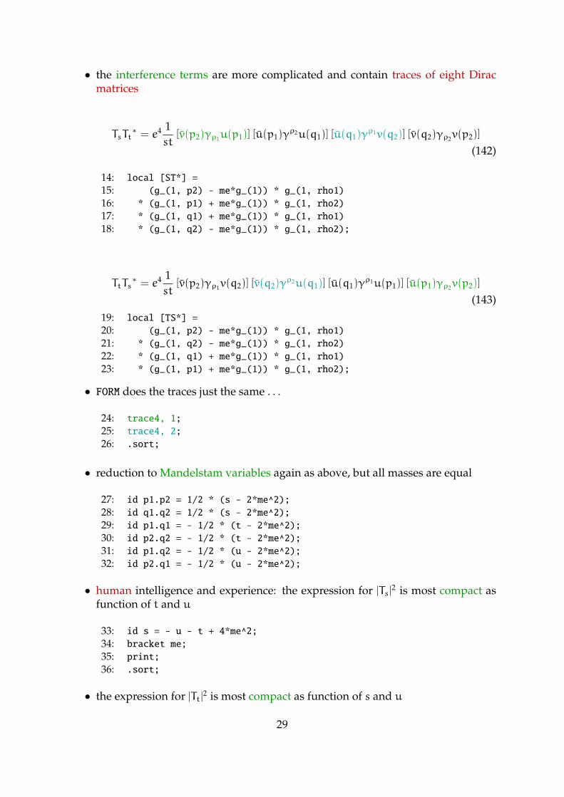
• the interference terms are more complicated and contain traces of eight Diracmatrices
TsTt∗ = e4 1
st[v(p2)γρ1u(p1)] [u(p1)γ
ρ2u(q1)] [u(q1)γρ1v(q2)] [v(q2)γρ2v(p2)]
(142)
14: local [ST*] =15: (g_(1, p2) - me*g_(1)) * g_(1, rho1)16: * (g_(1, p1) + me*g_(1)) * g_(1, rho2)17: * (g_(1, q1) + me*g_(1)) * g_(1, rho1)18: * (g_(1, q2) - me*g_(1)) * g_(1, rho2);
TtTs∗ = e4 1
st[v(p2)γρ1v(q2)] [v(q2)γ
ρ2u(q1)] [u(q1)γρ1u(p1)] [u(p1)γρ2v(p2)]
(143)
19: local [TS*] =20: (g_(1, p2) - me*g_(1)) * g_(1, rho1)21: * (g_(1, q2) - me*g_(1)) * g_(1, rho2)22: * (g_(1, q1) + me*g_(1)) * g_(1, rho1)23: * (g_(1, p1) + me*g_(1)) * g_(1, rho2);
• FORM does the traces just the same . . .
24: trace4, 1;25: trace4, 2;26: .sort;
• reduction to Mandelstam variables again as above, but all masses are equal
27: id p1.p2 = 1/2 * (s - 2*me^2);28: id q1.q2 = 1/2 * (s - 2*me^2);29: id p1.q1 = - 1/2 * (t - 2*me^2);30: id p2.q2 = - 1/2 * (t - 2*me^2);31: id p1.q2 = - 1/2 * (u - 2*me^2);32: id p2.q1 = - 1/2 * (u - 2*me^2);
• human intelligence and experience: the expression for |Ts|2 is most compact as
function of t and u
33: id s = - u - t + 4*me^2;34: bracket me;35: print;36: .sort;
• the expression for |Tt|2 is most compact as function of s and u
29
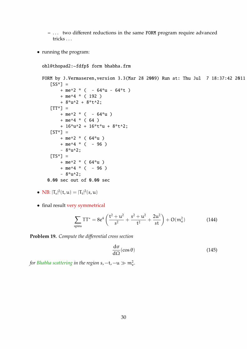
– . . . two different reductions in the same FORM program require advancedtricks . . .
• running the program:
ohl@thopad2:~fdfp$ form bhabha.frm
FORM by J.Vermaseren,version 3.3(Mar 28 2009) Run at: Thu Jul 7 18:37:42 2011[SS*] =
+ me^2 * ( - 64*u - 64*t )+ me^4 * ( 192 )+ 8*u^2 + 8*t^2;
[TT*] =+ me^2 * ( - 64*u )+ me^4 * ( 64 )+ 16*u^2 + 16*t*u + 8*t^2;
[ST*] =+ me^2 * ( 64*u )+ me^4 * ( - 96 )- 8*u^2;
[TS*] =+ me^2 * ( 64*u )+ me^4 * ( - 96 )- 8*u^2;
0.00 sec out of 0.00 sec
• NB: |Ts|2(t,u) = |Tt|2(s,u)
• final result very symmetrical
∑spins
TT∗ = 8e4(t2 + u2
s2 +s2 + u2
t2 +2u2
st
)+O(m2
e) (144)
Problem 19. Compute the differential cross section
dσdΩ
(cos θ) (145)
for Bhabha scattering in the region s,−t,−u m2e.
30
5 QCD
5.1 Feynman Rules
∵ full account requires another full set of lectures
∴ just a few SU(N) formulae
– generators Ta and totally anti symmetric structure constants fabc:
[Ta, Tb] = ifabcTc (146)
(summations for c = 1, 2, . . . , (N2c − 1) implied).
– normalization and contractions
tr (TaTb) =12δab (147a)
TaTa = CF · 1 =N2C − 12NC
· 1 (147b)
facdfbcd = CF · δab (147c)
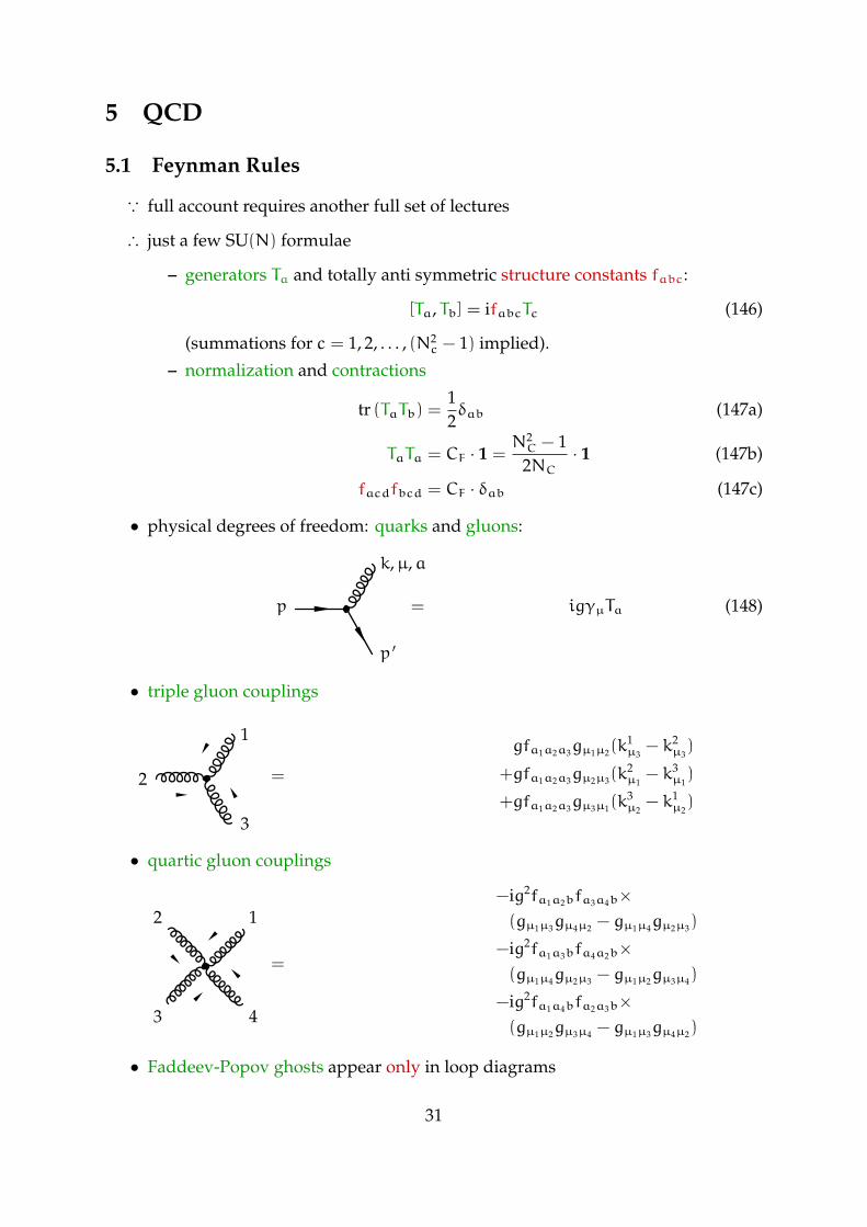
• physical degrees of freedom: quarks and gluons:
k,µ,a
p
p ′
= igγµTa (148)
• triple gluon couplings
1
2
3
=
gfa1a2a3gµ1µ2(k1µ3
− k2µ3)
+gfa1a2a3gµ2µ3(k2µ1
− k3µ1)
+gfa1a2a3gµ3µ1(k3µ2
− k1µ2)
(149)
• quartic gluon couplings
12
3 4
=
−ig2fa1a2bfa3a4b×(gµ1µ3gµ4µ2 − gµ1µ4gµ2µ3)
−ig2fa1a3bfa4a2b×(gµ1µ4gµ2µ3 − gµ1µ2gµ3µ4)
−ig2fa1a4bfa2a3b×(gµ1µ2gµ3µ4 − gµ1µ3gµ4µ2)
(150)
• Faddeev-Popov ghosts appear only in loop diagrams
31
5.2 3-Jet Production
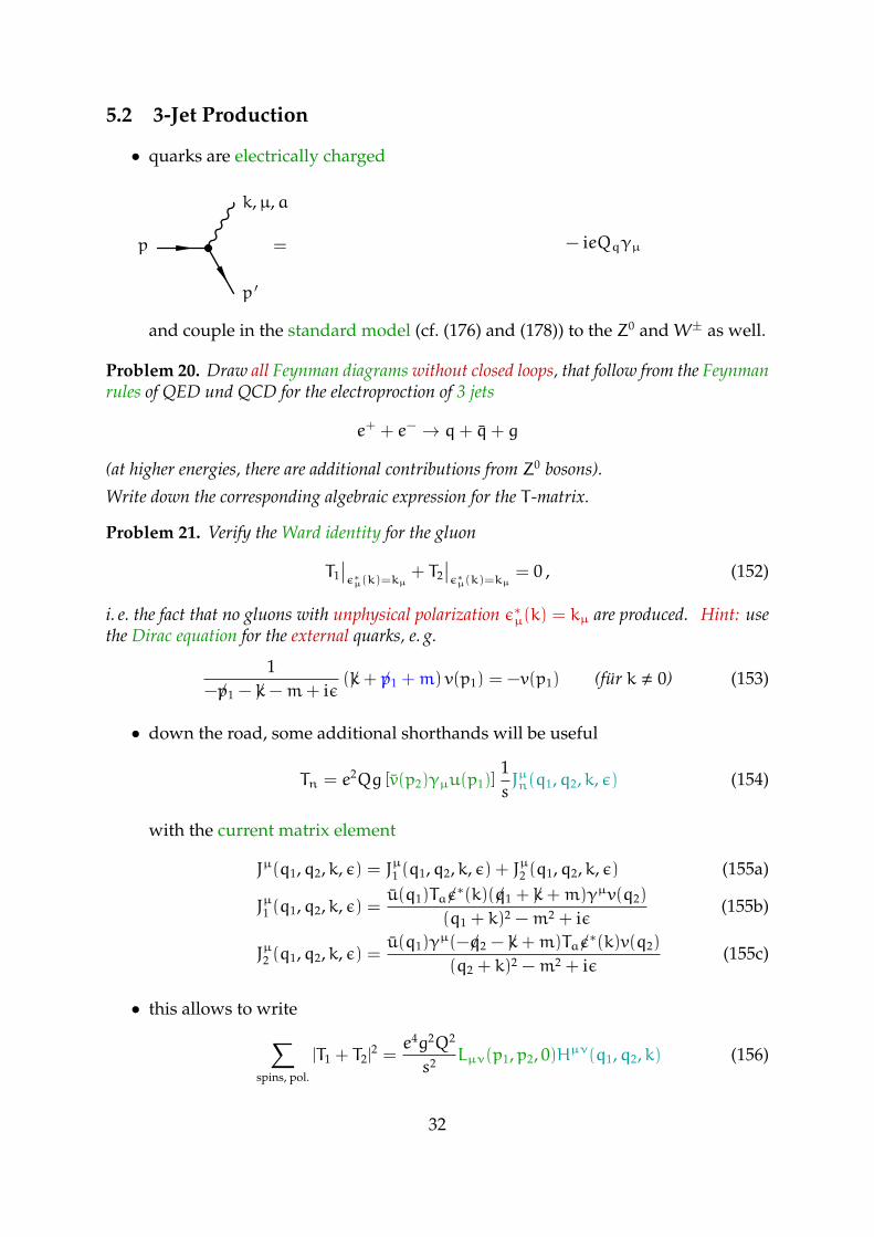
• quarks are electrically charged
k,µ,a
p
p ′
= − ieQqγµ (151)
and couple in the standard model (cf. (176) and (178)) to the Z0 andW± as well.
Problem 20. Draw all Feynman diagrams without closed loops, that follow from the Feynmanrules of QED und QCD for the electroproction of 3 jets
e+ + e− → q+ q+ g
(at higher energies, there are additional contributions from Z0 bosons).
Write down the corresponding algebraic expression for the T -matrix.
Problem 21. Verify the Ward identity for the gluon
T1∣∣ε∗µ(k)=kµ
+ T2∣∣ε∗µ(k)=kµ
= 0 , (152)
i. e. the fact that no gluons with unphysical polarization ε∗µ(k) = kµ are produced. Hint: usethe Dirac equation for the external quarks, e. g.
1−/p1 − /k−m+ iε
(/k+ /p1 +m) v(p1) = −v(p1) (für k , 0) (153)
• down the road, some additional shorthands will be useful
Tn = e2Qg [v(p2)γµu(p1)]1sJµn(q1,q2,k, ε) (154)
with the current matrix element
Jµ(q1,q2,k, ε) = Jµ1 (q1,q2,k, ε) + Jµ2 (q1,q2,k, ε) (155a)
Jµ1 (q1,q2,k, ε) =u(q1)Ta/ε
∗(k)(/q1 + /k+m)γµv(q2)
(q1 + k)2 −m2 + iε(155b)
Jµ2 (q1,q2,k, ε) =u(q1)γ
µ(−/q2 − /k+m)Ta/ε∗(k)v(q2)
(q2 + k)2 −m2 + iε(155c)
• this allows to write∑spins, pol.
|T1 + T2|2 =
e4g2Q2
s2 Lµν(p1,p2, 0)Hµν(q1,q2,k) (156)
32
with the “hadronic tensor”
Hµν(q1,q2,k) =∑
spins,ε
Jµ(q1,q2,k, ε)Jν,∗(q1,q2,k, ε) (157)
∵ with the same trick as in problem 21, we can show that
[qµ1 + qµ2 + kµ] Jµ(q1,q2,k, ε) = 0 (158)
∴ using the center of mass momentum p = p1 + p2 = q1 + q2 + k
pµHµν(q1,q2,k) = pνHµν(q1,q2,k) = 0 (159)
• angular dependence of Hµν(q1,q2,k) contains a lot of information . . .
∵ . . . but the energy dependence is much simpler
x1 = 2q1p/p2, x2 = 2q2p/p
2, x3 = 2kp/p2 (160)
∴ integrate over the angles
∫dq1dq2dk (2π)4δ4(q1 + q2 + k− p) f(x1, x2, x3)
=s
128π3
∫dx1dx2 f(x1, x2, 2 − x1 − x2) (161)
afterwards, thre result will depend only on p and the xi.
∵ from (159) we find∫dΩHµν(q1,q2,k) =
(pµpν
p2 − gµν)H(p, x1, x2) (162)
∴
H(p, x1, x2) = −13
∫dΩHµµ(q1,q2,k) (163)
• energy conservation
x1 + x2 + x3 =2(q1 + q2 + k)p
p2 = 2 (164)
• momentum conservation for massless particles
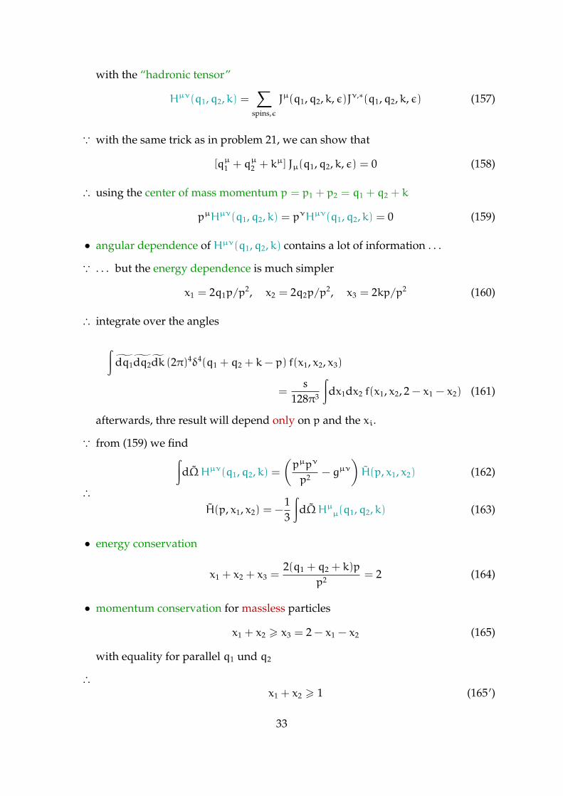
x1 + x2 > x3 = 2 − x1 − x2 (165)
with equality for parallel q1 und q2
∴x1 + x2 > 1 (165 ′)
33
0 0.2 0.4 0.6 0.8 10
0.2
0.4
0.6
0.8
1
x3 = 1
x3 = 0
x1
x2
• for massless particles
∑spins, pol.
∫dΩ |T1 + T2|
2 =4e4g2Q2
s2 (pµ1 pν2 + pν1 p
µ2 − p1p2g
µν)
×(pµpν
s− gµν
)H(p, x1, x2) =
4e4g2Q2
sH(p, x1, x2) (166)
• add phase space factor
d2σ
dx1dx2=
12s
s
128π3
14
∑spins, pol.
∫dΩ |T1 + T2|
2 =αsα
2Q2
4sH(p, x1, x2) (167)
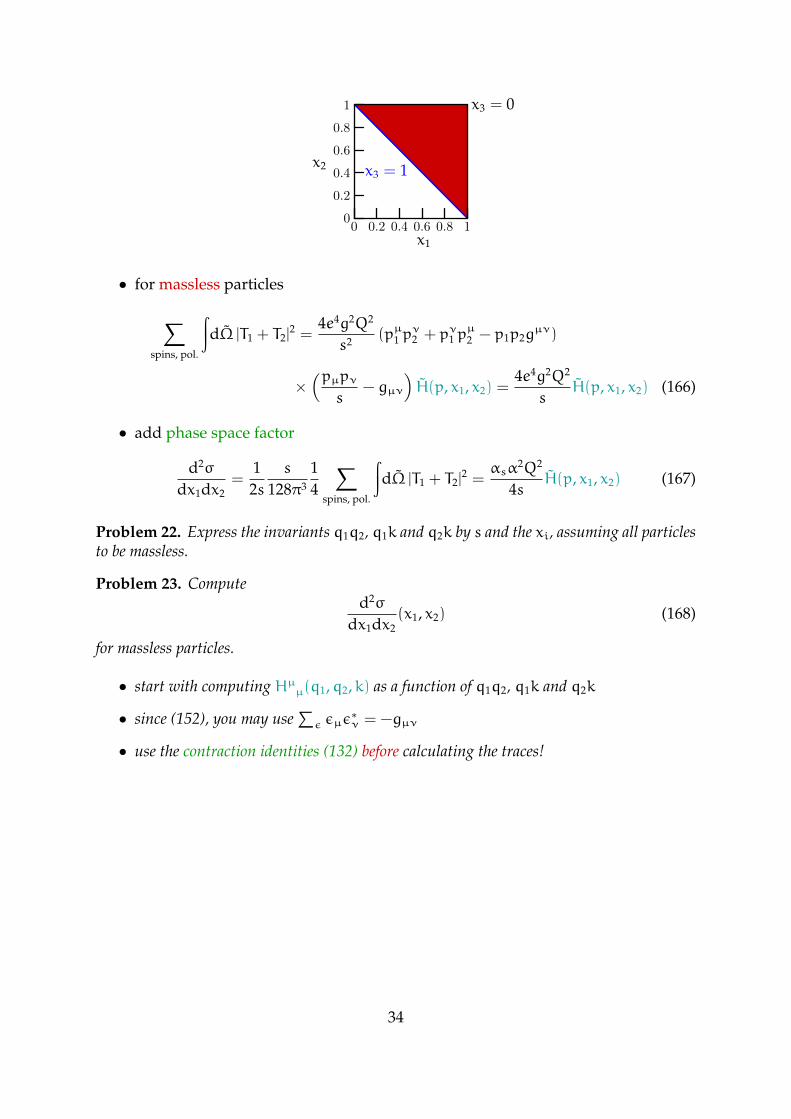
Problem 22. Express the invariants q1q2, q1k and q2k by s and the xi, assuming all particlesto be massless.
Problem 23. Computed2σ
dx1dx2(x1, x2) (168)
for massless particles.
• start with computing Hµµ(q1,q2,k) as a function of q1q2, q1k and q2k
• since (152), you may use∑ε εµε
∗ν = −gµν
• use the contraction identities (132) before calculating the traces!
34
6 Standard Model
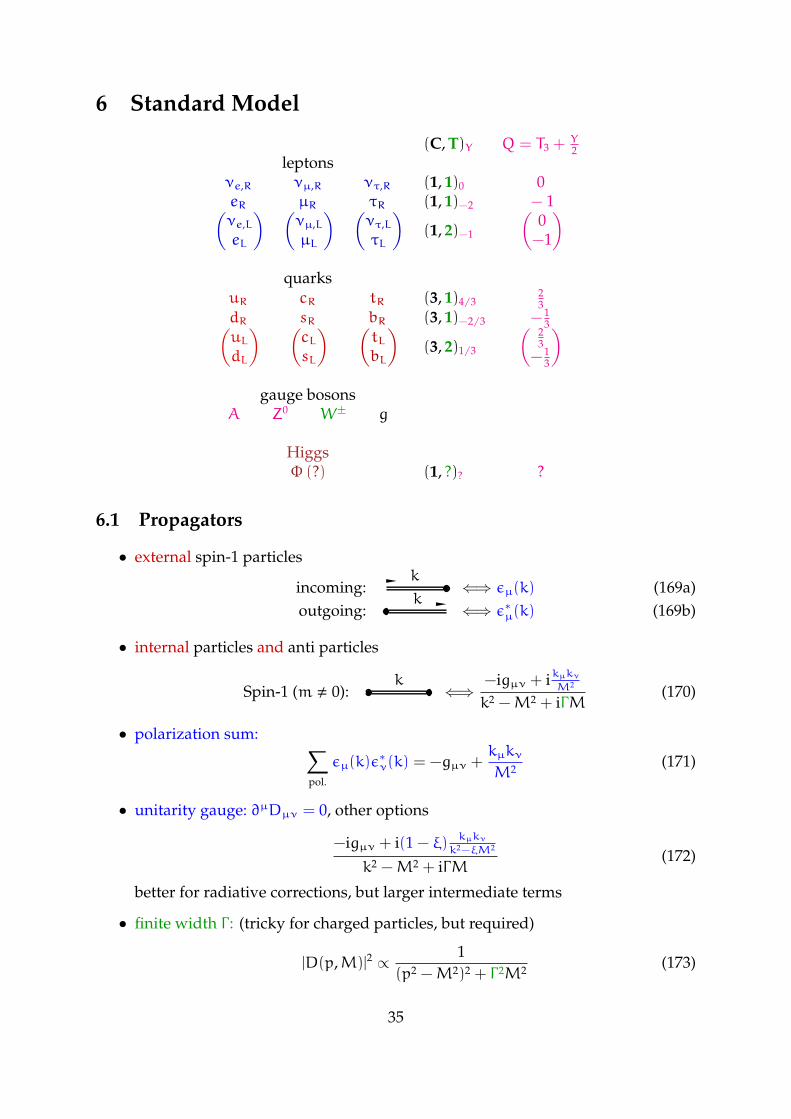
(C, T)Y Q = T3 +Y2
leptonsνe,R νµ,R ντ,R (1, 1)0 0eR µR τR (1, 1)−2 − 1(νe,L
eL
) (νµ,L
µL
) (ντ,L
τL
)(1, 2)−1
(0−1
)quarks
uR cR tR (3, 1)4/323
dR sR bR (3, 1)−2/3 −13(
uLdL
) (cLsL
) (tLbL
)(3, 2)1/3
( 23−1
3
)gauge bosons
A Z0 W± g
HiggsΦ (?) (1, ?)? ?
6.1 Propagators
• external spin-1 particles
incoming:k
⇐⇒ εµ(k) (169a)outgoing:
k⇐⇒ ε∗µ(k) (169b)
• internal particles and anti particles
Spin-1 (m , 0):k
⇐⇒−igµν + ikµkν
M2
k2 −M2 + iΓM(170)
• polarization sum: ∑pol.
εµ(k)ε∗ν(k) = −gµν +
kµkν
M2 (171)
• unitarity gauge: ∂µDµν = 0, other options
−igµν + i(1 − ξ)kµkνk2−ξM2
k2 −M2 + iΓM(172)
better for radiative corrections, but larger intermediate terms
• finite width Γ : (tricky for charged particles, but required)
|D(p,M)|2 ∝ 1(p2 −M2)2 + Γ 2M2 (173)
35
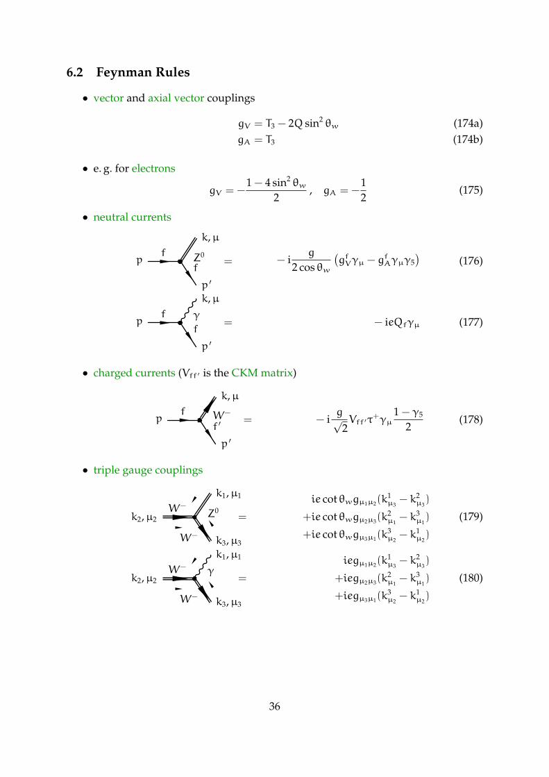
6.2 Feynman Rules
• vector and axial vector couplings
gV = T3 − 2Q sin2 θw (174a)gA = T3 (174b)
• e. g. for electrons
gV = −1 − 4 sin2 θw
2, gA = −
12
(175)
• neutral currents
f Z0
f
k,µ
p
p ′
= − ig
2 cos θw
(gfVγµ − g
fAγµγ5
)(176)
f γ
f
k,µ
p
p ′
= − ieQfγµ (177)
• charged currents (Vff ′ is the CKM matrix)
f W−
f ′
k,µ
p
p ′
= − ig√
2Vff ′τ
+γµ1 − γ5
2(178)
• triple gauge couplings
W−
Z0
W−
k1,µ1
k2,µ2
k3,µ3
=
ie cot θwgµ1µ2(k1µ3
− k2µ3)
+ie cot θwgµ2µ3(k2µ1
− k3µ1)
+ie cot θwgµ3µ1(k3µ2
− k1µ2)
(179)
W− γ
W−
k1,µ1
k2,µ2
k3,µ3
=
iegµ1µ2(k1µ3
− k2µ3)
+iegµ2µ3(k2µ1
− k3µ1)
+iegµ3µ1(k3µ2
− k1µ2)
(180)
36
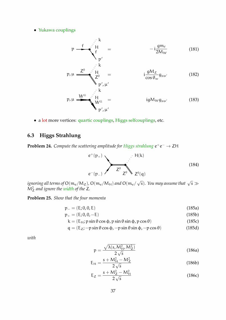
• Yukawa couplings
f Hf
k
p
p ′
= − igmf
2MW(181)
Z0HZ0
k
p,µ
p ′,µ ′
= igMZ
cos θwgµµ ′ (182)
W± HW±
k
p,µ
p ′,µ ′
= igMWgµµ ′ (183)
• a lot more vertices: quartic couplings, Higgs selfcouplings, etc.
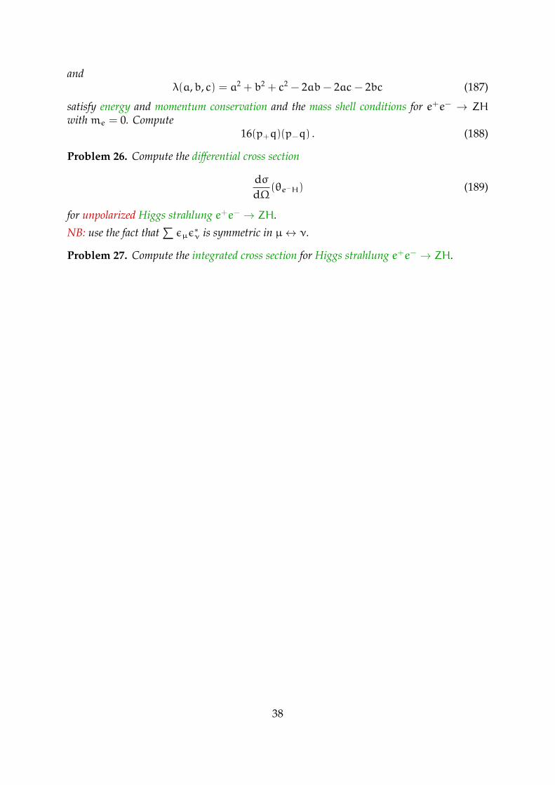
6.3 Higgs Strahlung
Problem 24. Compute the scattering amplitude for Higgs strahlung e+e− → ZH
Z0
Z0e−(p−)
e+(p+)
Z0(q)
H(k)
(184)
ignoring all terms ofO(me/MZ),O(me/MH) andO(me/√s). You may assume that
√s
M2Z and ignore the width of the Z.
Problem 25. Show that the four momenta
p− = (E; 0, 0,E) (185a)p+ = (E; 0, 0,−E) (185b)k = (EH;p sin θ cosφ,p sin θ sinφ,p cos θ) (185c)q = (EZ;−p sin θ cosφ,−p sin θ sinφ,−p cos θ) (185d)
with
p =
√λ(s,M2
H,M2Z)
2√s
(186a)
EH =s+M2
H −M2Z
2√s
(186b)
EZ =s+M2
Z −M2H
2√s
(186c)
37
andλ(a,b, c) = a2 + b2 + c2 − 2ab− 2ac− 2bc (187)
satisfy energy and momentum conservation and the mass shell conditions for e+e− → ZH
withme = 0. Compute16(p+q)(p−q) . (188)
Problem 26. Compute the differential cross section
dσdΩ
(θe−H) (189)
for unpolarized Higgs strahlung e+e− → ZH.
NB: use the fact that∑εµε
∗ν is symmetric in µ↔ ν.
Problem 27. Compute the integrated cross section for Higgs strahlung e+e− → ZH.
38
7 Solutions
Solution 1.
∂µe−ipx = −ipµe−ipx (190a)
(a∂)(b∂)e−ipx = −(ap)(bp)e−ipx (190b)
∂2e−ipx = −i(p∂)e−ipx = −p2e−ipx (190c)
Solution 2.
∂µxµ = g ν
µ ∂xµ/∂xν = g ν
µ δµν = g µ
µ = 4 (191a)
∂2e−x2/2 = −∂µ
(xµe−x
2/2)= −xµ∂
µe−x2/2 − (∂µxµ) e−x
2/2
= xµxµe−x
2/2 − g µµ e−x
2/2 = (x2 − 4)e−x2/2 (191b)
Solution 3.
[γk,γl
]+=
(0 σk
−σk 0
)(0 σl
−σl 0
)+ (k←→ l) =
(−σkσl 0
0 −σkσl
)+ (k←→ l)
=
(−[σk,σl]+ 0
0 −[σk,σl]+
)= −2δkl
(1 00 1
)(192a)
Solution 4.
uk(p) = u†k(p)γ0 = u
†k(~0)γ0γ0 /p† +m√
p0 +mγ0 = uk(~0)
/p+m√p0 +m
(193a)
vk(p) = vk(~0)/p−m√p0 +m
(193b)
Using the definition and multiplying with γ0 from the right
2∑k=1
uk(~0)uk(~0) =γ0 + 1
2,
2∑k=1
vk(~0)vk(~0) =γ0 − 1
2(194)
39
Therefore
2∑k=1
uk(p)uk(p) =(/p+m) (γ0 + 1) (/p+m)
2(p0 +m)(195a)
2∑k=1
vk(p)vk(p) =(/p−m) (γ0 − 1) (/p−m)
2(p0 +m)(195b)
and (60) follows from
(/p±m)(γ0 ± 1)(/p±m) = /pγ0/p± (mγ0/p+m/pγ0) +m2γ0 ± (/p±m)2
= −p2γ0 + 2p0/p± 2p0m+m2γ0 + 2m(/p±m) = 2(p0 +m)(/p±m) . (196)
Solution 5.
uk(p)ul(p) = uk(~0)/p+m√p0 +m
/p+m√p0 +m
ul(~0)
=2m
p0 +muk(~0)(/p+m)ul(~0)
=2m
p0 +muk(~0)(p0 +m)ul(~0) = 2muk(~0)ul(~0) = 2mδkl (197)
vk(p)vl(p) = vk(~0)/p−m√p0 +m
/p−m√p0 +m
vl(~0)
=−2mp0 +m
vk(~0)(/p−m)vl(~0)
=2m
p0 +mvk(~0)(p0 +m)vl(~0) = 2mvk(~0)vl(~0) = −2m · δkl (198)
uk(p)vl(p) = uk(~0)/p+m√p0 +m
/p−m√p0 +m
vl(~0) = 0 (199a)
vk(p)ul(p) = vk(~0)/p−m√p0 +m
/p+m√p0 +m
ul(~0) = 0 (199b)
40
Solution 6.
uk(p)γµul(p) = uk(~0)/p+m√p0 +m
γµ/p+m√p0 +m
ul(~0)
=1
p0 +muk(~0)2pµ(/p+m)ul(~0)
=2pµp0 +m
uk(~0)(p0 +m)ul(~0) = 2pµuk(~0)ul(~0) = 2pµδkl (200a)
vk(p)γµvl(p) = vk(~0)/p−m√p0 +m
γµ/p−m√p0 +m
vl(~0)
=1
p0 +mvk(~0)2pµ(/p−m)vl(~0)
=−2pµp0 +m
vk(~0)(p0 +m)vl(~0) = −2pµvk(~0)vl(~0) = 2pµδkl (200b)
uk(~p)γ0vl(−~p) = uk(~0)/p+m√p0 +m
γ0/p† −m√p0 +m
vl(~0)
= uk(~0)/p+m√p0 +m
/p−m√p0 +m
γ0vl(~0) = 0 (201a)
vk(−~p)γ0ul(~p) = 0 (201b)
Solution 7.
γ5γ2 = iγ0γ1γ2γ3γ2 = −iγ0γ1γ2γ2γ3 = iγ0γ2γ1γ2γ3 = −iγ2γ0γ1γ2γ3 = −γ2γ5 (202)
since every γµ appears exaclty once and anti-commutes with the other three, we have for every µ
[γ5,γµ]+ = 0 (203)
Solution 8.
product rule
i∂µ[ψ1(x)γµψ2(x)
]= ψ1(x)
(i←−/∂ + i
−→/∂)ψ2(x) = ψ1(x)
(−m+m
)ψ2(x) = 0 . (204)
41
Solution 9.
product rule and [γ5,γµ]+ = 0
i∂µ[ψ1(x)γµγ5ψ2(x)
]= ψ1(x)
(i←−/∂ γ5 + i
−→/∂ γ5
)ψ2(x) = ψ1(x)
(i←−/∂ γ5 − γ5i
−→/∂)ψ2(x)
= ψ1(x)(−mγ5 − γ5m
)ψ2(x) = −2mψ1(x)γ5ψ2(x) . (205)
Solution 10.
− 2iσkl =(
0 σk
−σk 0
)(0 σl
−σl 0
)− (k←→ l)
=
(−[σk,σl]− 0
0 −[σk,σl]−
)= −2iεklm
(σm 00 σm
)(206)
therefore
σkl = εklm
(σm 00 σm
)(207)
Solution 11.
(i/∂−m)S(x,m) =(−∂2 −m2)D(x,m) = δ4(x) (208)
Solution 12.
S(x,m) = (i/∂+m)
∫d4p
(2π)4 e−ipx 1p2 −m2+iε
=
∫d4p
(2π)4 e−ipx /p+m
p2 −m2+iε=
∫d4p
(2π)4 e−ipx 1/p−m+iε
(209)
Solution 13.
tr (/a/b/c/d) = + tr (/b/c/d/a) = − tr (/b/c/a/d) + 2 · ad · tr (/b/c)= + tr (/b/a/c/d) − 2 · ac · tr (/b/d) + 2 · ad · 4 · bc
= − tr (/a/b/c/d) + 2 · ab · tr (/c/d) − 2 · ac · 4 · bd+ 2 · ad · 4 · bc
thereforetr (/a/b/c/d) = 4 · (ab · cd− ac · bd+ ad · bc) (133 ′)
42
Solution 14.
Lµν = tr [(/p+m)γµ(/q−m)γν] = tr [/pγµ/qγν] −m2 tr [γµγν]
= 4 · (pµqν − gµνpq+ pνqµ) − 4m2 · gµν = 4 ·(pµqν + pνqµ − (pq+m2)gµν
)(210)
Solution 15.
Lρ2ρ1Lρ1ρ2 = 16 · (p1,ρ2p2,ρ1 + p1,ρ1p2,ρ2 − p1p2gρ2ρ1)(q
ρ11 q
ρ22 + qρ2
1 qρ12 − q1q2g
ρ1ρ2)
= 8 ·(
2(p1q2)2(p2q1) + 2(p1q1)2(p2q2))= 8 ·
(u2 + t2
)(211)
NB: cross terms cancel:
(p1,ρ2p2,ρ1 + p1,ρ1p2,ρ2)q1q2gρ1ρ2 + p1p2gρ2ρ1(q
ρ11 q
ρ22 + qρ2
1 qρ12 ) = p1p2gρ2ρ1q1q2g
ρ1ρ2
Solution 16.
t = −s
2(1 − cos θ) , u = −
s
2(1 + cos θ) (212)
thereforet2 + u2
s2 =1 + cos2 θ
2(213)
dσ =1
4√
(p1p2)2 −m21m
22
1∏i ni!
14|T |
2dq1dq2(2π)4δ4(p1 + p2 − q1 − q2)
=1
4√
(s/2)2
14|T |
2 132π2 d cos θdφ =
164π2s
14|T |
2dΩ (214)
thereforedσdΩ
=1
64π2se4 (1 + cos2 θ
)= α2 1
4s(1 + cos2 θ
)(215)
Solution 17.
σ =
∫dΩ
dσdΩ
=α2
4s2π∫ 1
−1d cos θ
(1 + cos2 θ
)=α2
4s2π(
2 +23
)=
4πα2
3s(216)
compare
σ =4πα2
3(√s/TeV)2 0.39 nb (19 ′′)
with
α =e2
4π=
1137.0359895(61)
(217)
σ =87 fb
(√s/TeV)2 =
8.7 pb(√s/100 GeV)2 (19 ′′)
43
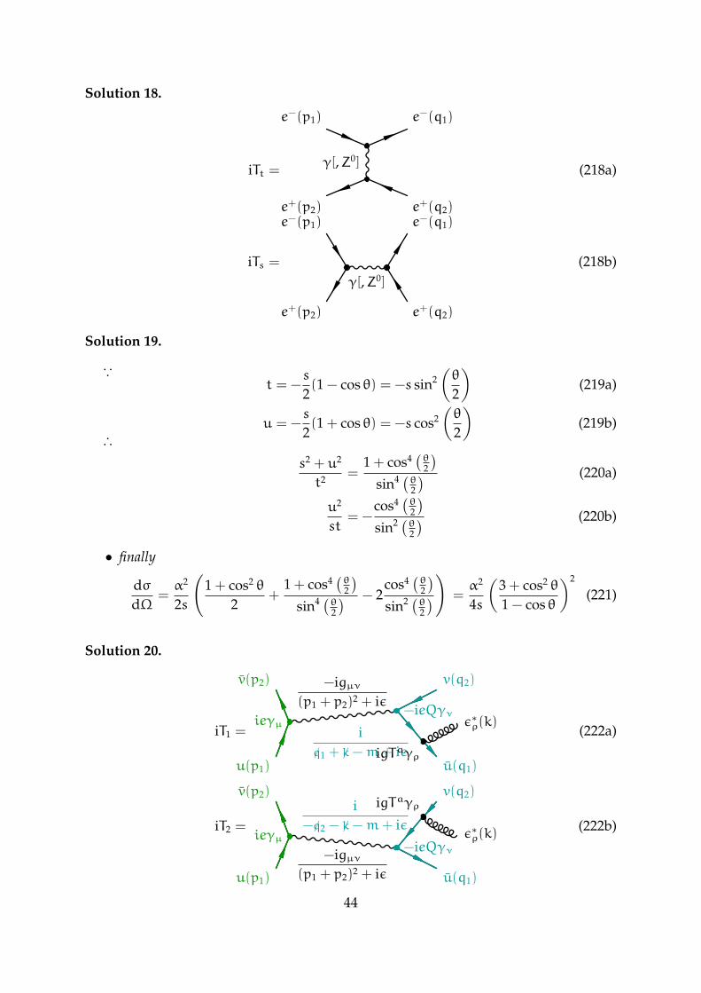
Solution 18.
iTt =γ[,Z0]
e+(p2)
e−(p1)
e+(q2)
e−(q1)
(218a)
iTs =γ[,Z0]
e+(p2)
e−(p1)
e+(q2)
e−(q1)
(218b)
Solution 19.
∵t = −
s
2(1 − cos θ) = −s sin2
(θ
2
)(219a)
u = −s
2(1 + cos θ) = −s cos2
(θ
2
)(219b)
∴
s2 + u2
t2 =1 + cos4
(θ2
)sin4 (θ
2
) (220a)
u2
st= −
cos4(θ2
)sin2 (θ
2
) (220b)
• finally
dσdΩ
=α2
2s
(1 + cos2 θ
2+
1 + cos4(θ2
)sin4 (θ
2
) − 2cos4
(θ2
)sin2 (θ
2
)) =α2
4s
(3 + cos2 θ
1 − cos θ
)2
(221)
Solution 20.
iT1 =
−igµν(p1 + p2)2 + iε
i/q1 + /k−m+ iε
u(p1)
v(p2)
u(q1)
ε∗ρ(k)
v(q2)
ieγµ−ieQγν
igTaγρ
(222a)
iT2 =
−igµν(p1 + p2)2 + iε
i−/q2 − /k−m+ iε
u(p1)
v(p2)
u(q1)
ε∗ρ(k)
v(q2)
ieγµ−ieQγν
igTaγρ(222b)
44
iT1 =
[u(q1)(igTa/ε
∗(k))i
/q1 + /k−m+ iε(−ieQγµ)v(q2)
]× (223a)
−i(p1 + p2)2 + iε
[v(p2)(ieγµ)u(p1)]
iT2 =
[u(q1)(−ieQγµ)
i−/q2 − /k−m+ iε
(igTa/ε∗(k))v(q2)
]× (223b)
−i(p1 + p2)2 + iε
[v(p2)(ieγµ)u(p1)]
Solution 21.
T1∣∣ε∗µ(k)=kµ
= e2Qg [v(p2)γµu(p1)]1su(q1)Ta(/k+ /q1 −m)
1/q1 + /k−m+ iε
γµv(q2)
= e2Qg [v(p2)γµu(p1)]1su(q1)Taγ
µv(q2) (224)
on the other hand
T2∣∣ε∗µ(k)=kµ
= e2Qg [v(p2)γµu(p1)]1su(q1)γ
µ 1−/q2 − /k−m+ iε
(/k+ /q2 +m)Tav(q2)
= −e2Qg [v(p2)γµu(p1)]1su(q1)Taγ
µv(q2) = −T1∣∣ε∗µ(k)=kµ
(225)
Solution 22.
2q1q2 = (q1 + q2)2 = (p− k)2 = s(1 − x3) (226a)
2q1k = (q1 + k)2 = (p− q2)
2 = s(1 − x2) (226b)
2q2k = (q2 + k)2 = (p− q1)
2 = s(1 − x1) (226c)
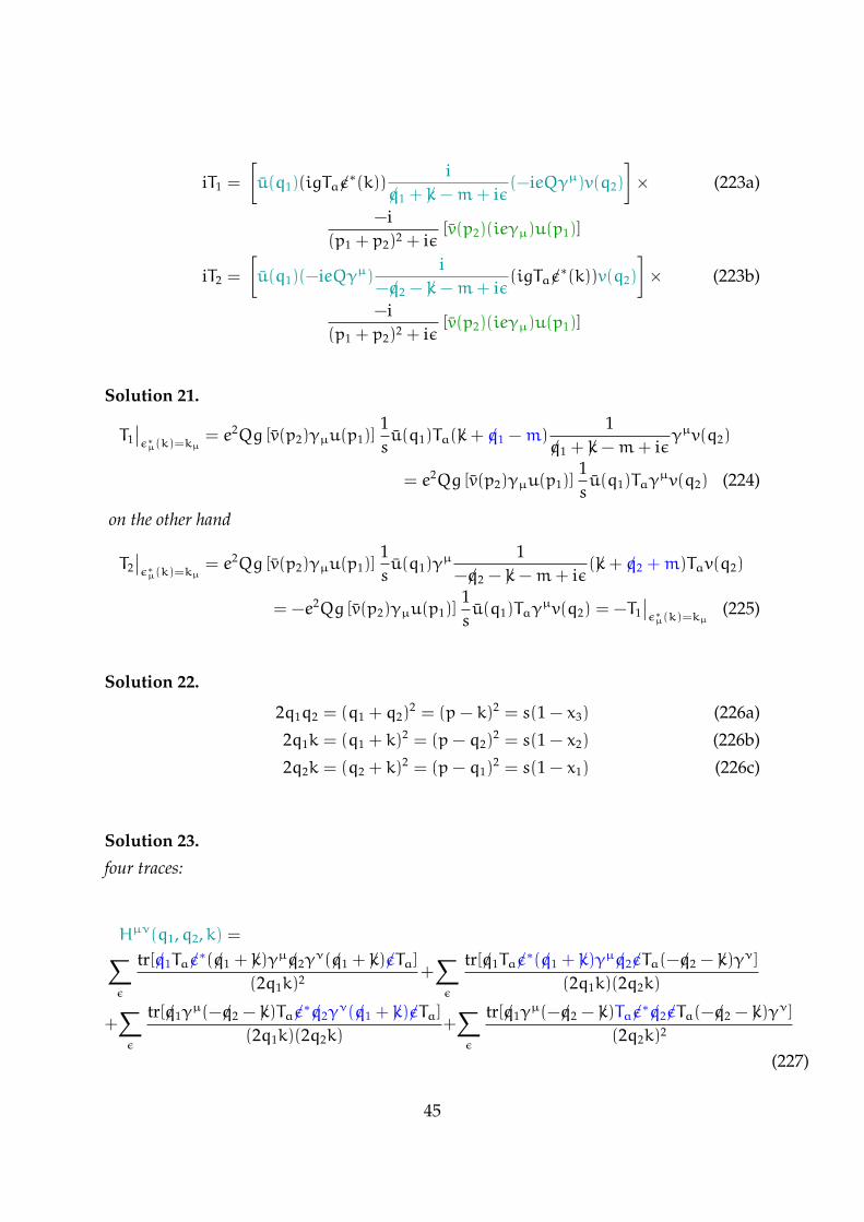
Solution 23.
four traces:
Hµν(q1,q2,k) =∑ε
tr[/q1Ta/ε∗(/q1 + /k)γ
µ/q2γν(/q1 + /k)/εTa]
(2q1k)2 +∑ε
tr[/q1Ta/ε∗(/q1 + /k)γ
µ/q2/εTa(−/q2 − /k)γν]
(2q1k)(2q2k)
+∑ε
tr[/q1γµ(−/q2 − /k)Ta/ε
∗/q2γν(/q1 + /k)/εTa]
(2q1k)(2q2k)+∑ε
tr[/q1γµ(−/q2 − /k)Ta/ε
∗/q2/εTa(−/q2 − /k)γν]
(2q2k)2
(227)
45
color part of the quark traces tr(TaTa) = CF tr(1) = CFNC and polarization sum
Hµν(q1,q2,k) = 2CFNctr[/q1(/q1 + /k)γ
µ/q2γν(/q1 + /k)]
(2q1k)2 +2CFNctr[/q1/q2γ
µ(/q1 + /k)(−/q2 − /k)γν]
(2q1k)(2q2k)
+ 2CFNctr[/q1γ
µ(−/q2 − /k)(/q1 + /k)γν/q2]
(2q1k)(2q2k)+ 2CFNc
tr[/q1γµ(−/q2 − /k)/q2(−/q2 − /k)γ
ν]
(2q2k)2
(228)
contraction
Hµµ(q1,q2,k) = −4CFNctr[/q1(/q1 + /k)/q2(/q1 + /k)]
(2q1k)2 +8CFNc(q1+k)(−q2−k)tr[/q1/q2]
(2q1k)(2q2k)
+ 8CFNc(−q2 − k)(q1 + k)tr[/q1/q2]
(2q1k)(2q2k)− 4CFNc
tr[/q1(−/q2 − /k)/q2(−/q2 − /k)]
(2q2k)2 (229)
final traces
Hµµ(q1,q2,k) = −16CFNc2(q1k)(q2k)
(2q1k)2 −64CFNc(q1q2 + q1k+ q2k)(q1q2)
(2q1k)(2q2k)−16CFNc
2(q1k)(q2k)
(2q2k)2
−8CFNc1 − x1
1 − x2−16CFNc
(1 − x3)
(1 − x1)(1 − x2)−8CFNc
1 − x2
1 − x1= −8CFNc
x21 + x
22
(1 − x1)(1 − x2)(230)
resultd2σ
dx1dx2= Nc
4πα2Q2
3sαs
2πCF
x21 + x
22
(1 − x1)(1 − x2)(231)
Solution 24.
with p = p+ + p−:
iT = −ig
2 cos θw[v(p+)γµ(g
eV − geAγ5)u(p−)]
−igµν + ipµpν/M2Z
p2 −M2Z
(igMZ
cos θwgνρ)ε
∗,ρ(q)
(232)and from current conservation [v(p+)γµ(g
eV − geAγ5)u(p−)]p
µ = −2igeAmev(p+)γ5u(p−) =O(me)
T = −g2MZ
2 cos2 θw
1s−M2
Z
[v(p+)/ε∗(q)(geV − geAγ5)u(p−)] (233)
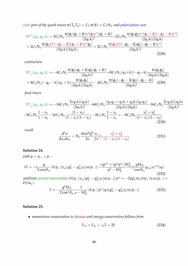
Solution 25.
• momentum conservation is obvious and energy conservation follows from
EH + EZ =√s = 2E (234)
46
• the Higgs mass shell follows from
E2H − p2 =
s2 +M4H +M4
Z+2sM2H − 2sM2
Z − 2M2HM
2Z
4s
−s2 +M4
H +M4Z−2sM2
H − 2sM2Z − 2M2
HM2Z
4s=M2
H , (235)
and the Z mass shell analogously: E2Z − p2 =M2
Z.
• finally
4p∓q = 4E(EZ ± p cos θ) = s+M2Z −M2
H ±√λ(s,M2
H,M2Z) cos θ , (236)
i. e.
16(p+q)(p−q) = (s+M2Z −M2
H)2 − λ(s,M2
H,M2Z) cos2 θ
= 4sM2Z + λ(s,M2
H,M2Z) sin2 θ (237)
Solution 26.
∑spins
|T |2 =g4M2
Z
4 cos4 θw
1(s−M2
Z)2
tr (/p+/ε∗(q)(geV − geAγ5)/p−(geV + geAγ5)/ε(q))
=g4M2
Z
4 cos4 θw
1(s−M2
Z)2(geV
2 + geA2) tr (/p+/ε∗(q)/p−/ε(q))
=g4M2
Z(geV
2 + geA2)
4 cos4 θw
1(s−M2
Z)2Lµν(p+,p−, 0)ε∗µ(q)εν(q) (238)
polarization sum ∑pol.
εµ(q)ε∗ν(q) = −gµν +
qµqν
M2Z
(239)
∑spins, pol.
|T |2 =g4M2
Z(geV
2 + geA2)
cos4 θw
1(s−M2
Z)2
(pµ+p
ν− + pµ−p
ν+ − p+p−g
µν)×
(−gµν +
qµqν
M2Z
)=g4(geV
2 + geA2)
cos4 θw
p+p−M2Z + 2(p+q)(p−q)(s−M2
Z)2
=g4(geV
2 + geA2)
8 cos4 θw
8sM2Z + λ(s,M2
H,M2Z) sin2 θ
(s−M2Z)
2(240)
47
phase space (118)
dσdΩ
(θe−H) =12s
116π2
√λ(s,M2
H,M2Z)
2s14
∑spins, pol.
|T |2 (241)
i. e.
dσdΩ
(θe−H) =
√λ(s,M2
H,M2Z)
s
α2(geV2 + geA
2)
128s sin4 θw cos4 θw
8sM2Z + λ(s,M2
H,M2Z) sin2 θ
(s−M2Z)
2(242)
Solution 27.
with ∫dΩ (a+ b sin2 θ) = 4πa+
8π3b (243)
follows
σ =
√λ(s,M2
H,M2Z)
s
πα2(geV2 + geA
2)
48s sin4 θw cos4 θw
12sM2Z + λ(s,M2
H,M2Z)
(s−M2Z)
2(244)
or
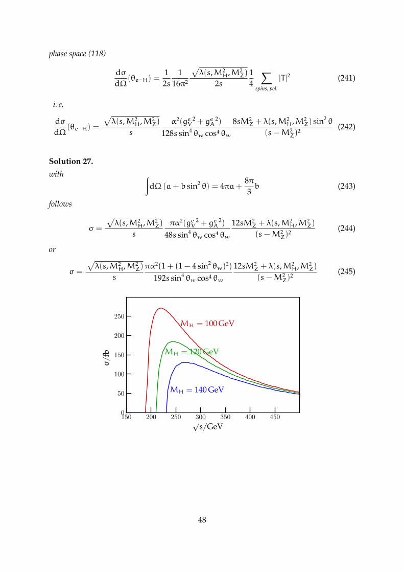
σ =
√λ(s,M2
H,M2Z)
s
πα2(1 + (1 − 4 sin2 θw)2)
192s sin4 θw cos4 θw
12sM2Z + λ(s,M2
H,M2Z)
(s−M2Z)
2(245)
MH = 100 GeV
MH = 120 GeV
MH = 140 GeV
150 200 250 300 350 400 4500
50
100
150
200
250
√s/GeV
σ/
fb
48