2. TTA / TTT - Diagrams - KAUmercury.kau.ac.kr/welding/Welding Technology II - Welding... · 2. TTA...

2.

TTA / TTT - Diagrams

2. TTA / TTT – Diagrams 9

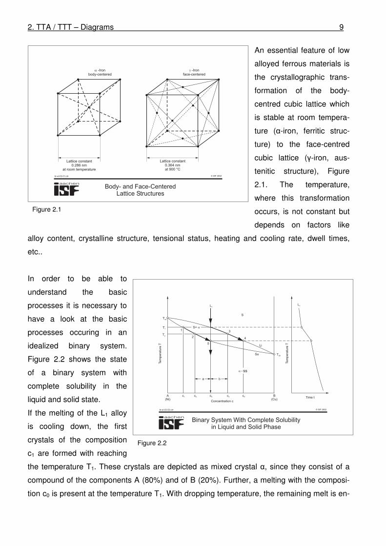
An essential feature of low

alloyed ferrous materials is

the crystallographic trans-

formation of the body-

centred cubic lattice which

is stable at room tempera-

ture (α-iron, ferritic struc-

ture) to the face-centred

cubic lattice (γ-iron, aus-

tenitic structure), Figure

2.1. The temperature,

where this transformation

occurs, is not constant but

depends on factors like

alloy content, crystalline structure, tensional status, heating and cooling rate, dwell times,

etc..

In order to be able to

understand the basic

processes it is necessary to

have a look at the basic

processes occuring in an

idealized binary system.

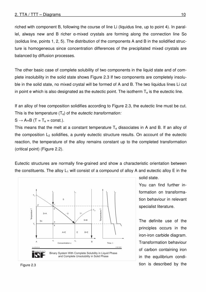
Figure 2.2 shows the state

of a binary system with

complete solubility in the

liquid and solid state.

If the melting of the L1 alloy

is cooling down, the first

crystals of the composition

c1 are formed with reaching

the temperature T1. These crystals are depicted as mixed crystal α, since they consist of a

compound of the components A (80%) and of B (20%). Further, a melting with the composi-

tion c0 is present at the temperature T1. With dropping temperature, the remaining melt is en-

© ISF 2002br-eI-02-01.cdr

Body- and Face-CenteredLattice Structures

Lattice constant0.286 nm

at room temperature

Lattice constant0.364 nmat 900 °C

a -Ironbody-centered

g -Ironface-centered

Figure 2.1


Binary System With Complete Solubilityin Liquid and Solid Phase

1

2

3

4

5

S

Li

So

A(Ni)

B(Cu)

L1L1

TsA

T1

T2

TsB

c1 c2 c3 c4c0 Time t

Tem

pera

ture

T

Tem

pera

ture

T

Concentration c

S+ a

a -

ba

ss

Figure 2.2


riched with component B, following the course of line Li (liquidus line, up to point 4). In paral-

lel, always new and B richer α-mixed crystals are forming along the connection line So

(solidus line, points 1, 2, 5). The distribution of the components A and B in the solidified struc-

ture is homogeneous since concentration differences of the precipitated mixed crystals are

balanced by diffusion processes.

The other basic case of complete solubility of two components in the liquid state and of com-

plete insolubility in the solid state shows Figure 2.3 If two components are completely insolu-

ble in the solid state, no mixed crystal will be formed of A and B. The two liquidus lines Li cut

in point e which is also designated as the eutectic point. The isotherm Te is the eutectic line.

If an alloy of free composition solidifies according to Figure 2.3, the eutectic line must be cut.

This is the temperature (Te) of the eutectic transformation:

S → A+B (T = Te = const.).

This means that the melt at a constant temperature Te dissociates in A and B. If an alloy of

the composition L2 solidifies, a purely eutectic structure results. On account of the eutectic

reaction, the temperature of the alloy remains constant up to the completed transformation

(critical point) (Figure 2.2).

Eutectic structures are normally fine-grained and show a characteristic orientation between

the constituents. The alloy L1 will consist of a compound of alloy A and eutectic alloy E in the

solid state.

You can find further in-

formation on transforma-

tion behaviour in relevant

specialist literature.

The definite use of the

principles occurs in the

iron-iron carbide diagram.

Transformation behaviour

of carbon containing iron

in the equilibrium condi-

tion is described by the


Binary System With Complete Solubility in Liquid Phaseand Complete Unsolubility in Solid Phase

TsA

Te

2’

L1 L1L2 L2

1

2

3

4

S+A

So

S

S+B

Li Li

A+E E B+E

B

TsB

c1 ce

Tem

pe

ratu

reT

Te

mp

era

ture

T

Concentration c Time tA

Figure 2.3


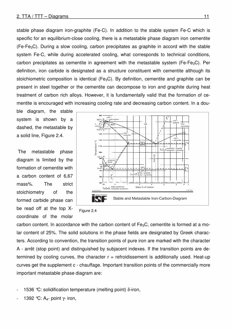
stable phase diagram iron-graphite (Fe-C). In addition to the stable system Fe-C which is

specific for an equilibrium-close cooling, there is a metastable phase diagram iron cementite

(Fe-Fe3C). During a slow cooling, carbon precipitates as graphite in accord with the stable

system Fe-C, while during accelerated cooling, what corresponds to technical conditions,

carbon precipitates as cementite in agreement with the metastable system (Fe-Fe3C). Per

definition, iron carbide is designated as a structure constituent with cementite although its

stoichiometric composition is identical (Fe3C). By definition, cementite and graphite can be

present in steel together or the cementite can decompose to iron and graphite during heat

treatment of carbon rich alloys. However, it is fundamentally valid that the formation of ce-

mentite is encouraged with increasing cooling rate and decreasing carbon content. In a dou-

ble diagram, the stable

system is shown by a

dashed, the metastable by

a solid line, Figure 2.4.

The metastable phase

diagram is limited by the

formation of cementite with

a carbon content of 6,67

mass%. The strict

stoichiometry of the

formed carbide phase can

be read off at the top X-

coordinate of the molar

carbon content. In accordance with the carbon content of Fe3C, cementite is formed at a mo-

lar content of 25%. The solid solutions in the phase fields are designated by Greek charac-

ters. According to convention, the transition points of pure iron are marked with the character

A - arrêt (stop point) and distinguished by subjacent indexes. If the transition points are de-

termined by cooling curves, the character r = refroidissement is additionally used. Heat-up

curves get the supplement c - chauffage. Important transition points of the commercially more

important metastable phase diagram are:

- 1536 °C: solidification temperature (melting point) δ-iron,

- 1392 °C: A4- point γ- iron,

Stable and Metastable Iron-Carbon-Diagram


melt +

- solid solutiond

d -+g-solid sol.

d -solid sol.

melt

melt +graphite

Fe C

(cementite)3

melt +cementite

melt +austenite

austenite

austenite + graphiteaustenite + cementite

ledeburite

austenite +ferrite

ferrite

perlite

stable equilibriummetastable equilibrium

ferrite + graphiteferrite + cementite

Mass % of Carbon

Tem

pera

ture

°C

Figure 2.4


- 911 °C: A3- point non-magnetic α- iron,

with carbon containing iron:

- 723 °C: A1- point (perlite point).

The corners of the phase fields are designated by continuous roman capital letters.

As mentioned before, the system iron-iron carbide is a more important phase diagram for

technical use and also for welding techniques. The binary system iron-graphite can be stabi-

lized by an addition of silicon so that a precipitation of graphite also occurs with increased

solidification velocity. Especially iron cast materials solidify due to their increased silicon con-

tents according to the stable system. In the following, the most important terms and transfor-

mations should be explained more closely as a case of the metastable system.

The transformation mechanisms explained in the previous sections can be found in the bi-

nary system iron-iron carbide almost without exception. There is an eutectic transformation in

point C, a peritectic one in point I, and an eutectoidic transformation in point S. With a tem-

perature of 1147°C and a carbon concentration of 4.3 mass%, the eutectic phase called Le-

deburite precipitates from cementite with 6,67% C and saturated γ-solid solutions with 2,06%

C. Alloys with less than 4,3 mass% C coming from primary austenite and Ledeburite are

called hypoeutectic, with more than 4,3 mass% C coming from primary austenite and Lede-

burite are called hypereutectic.

If an alloy solidifies with less than 0,51 mass percent of carbon, a δ-solid solution is formed

below the solidus line A-B (δ-ferrite). In accordance with the peritectic transformation at

1493°C, melt (0,51% C) and δ-ferrite (0,10% C) decompose to a γ-solid solution (austenite).

The transformation of the γ-solid solution takes place at lower temperatures. From γ-iron with

C-contents below 0.8% (hypoeutectoidic alloys), a low-carbon α-iron (pre-eutectoidic ferrite)

and a fine-lamellar solid solution (perlite) precipitate with falling temperature, which consists

of α-solid solution and cementite. With carbon contents above 0,8% (hypereutectoidic alloys)

secondary cementite and perlite are formed out of austenite. Below 723°C, tertiary cementite

precipitates out of the α-iron because of falling carbon solubility.


The most important distinguished feature of the three described phases is their lattice struc-

ture. α- and δ-phases are cubic body-centered (CBC lattice) and γ-phase is cubic face-

centered (CFC lattice), Figure 2.1.

Different carbon solubility of solid solutions also results from lattice structures. The three

above mentioned phases dissolve carbon interstitially, i.e. carbon is embedded between the

iron atoms. Therefore, this types of solid solutions are also named interstitial solid solution.

Although the cubic face-centred lattice of austenite has a higher packing density than the cu-

bic body-centred lattice, the void is bigger to disperse the carbon atom. Hence, an about 100

times higher carbon solubility of austenite (max. 2,06% C) in comparison with the ferritic

phase (max. 0,02% C for α-iron) is the result. However, diffusion speed in γ-iron is always at

least 100 times slower than in α-iron because of the tighter packing of the γ-lattice.

Although α- and δ-iron show the same lattice structure and properties, there is also a differ-

ence between these phases. While γ-iron develops of a direct decomposition of the melt (S

→ δ), α-iron forms in the solid phase through an eutectoidic transformation of austenite (γ →

α + Fe3C). For the transformation of non- and low-alloyed steels, is the transformation of δ-

ferrite of lower importance, although this δ-phase has a special importance for weldability of

high alloyed steels.

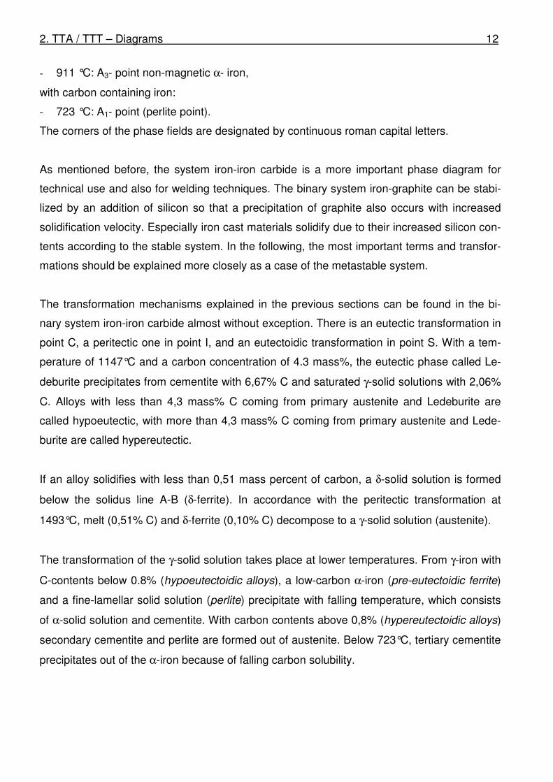
Unalloyed steels used in industry are multi-component systems of iron and carbon with alloy-

ing elements as manganese, chromium, nickel and silicon. Principally the equilibrium dia-

gram Fe-C applies also to

such multi-component sys-

tems. Figure 2.5 shows a

schematic cut through the

three phase system

Fe-M-C.

During precipitation, mixed

carbides of the general

composition M3C develop.

In contrast to the binary

system Fe-C, is the three Description of the Terms Ac , Ac , Ac1b 1e 3

Ac3

Ac1e


Figure 2.5


phase system Fe-M-C characterised by a temperature interval in the three-phase field α + γ +

M3C. The beginning of the transformation of α + M3C to γ is marked by Aclb, the end by Acle.

The indices b and e mean

the beginning and the end

of transformation.

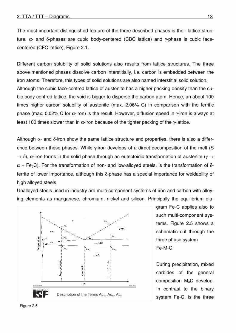
The described equilibrium

diagrams apply only to low

heating and cooling rates.

However, higher heating

and cooling rates are pre-

sent during welding, con-

sequently other structure

types develop in the heat

affected zone (HAZ) and in

the weld metal. The struc-

ture transformations during

heating and cooling are described by transformation diagrams, where a temperature change

is not carried out close to the equilibrium, but

at different heating and/or cooling rates.

A representation of the transformation

processes during isothermal austenitizing

shows Figure 2.6. This figure must be read

exclusively along the time axis! It can be

recognised that several transformations

during isothermal austenitizing occur with e.g.

800°C. Inhomogeneous austenite means

both, low carbon containing austenite is

formed in areas, where ferrite was present

before transformation, and carbon-rich aus-

tenite is formed in areas during transforma-

tion, where carbon was present before

transformation. During sufficiently long an-

nealing times, the concentration differences

are balanced by diffusion, the border to a ho-

TTA Diagram forIsothermal Austenitization


s

°C

Figure 2.6

TTA-Diagram forContinuous Warming

ASTM4; L=80µm ASTM11; L=7µm

20µm 20µm

© ISF 2002br-er02-07.cdr

Te

mp

era

ture

Time

Figure 2.7


mogeneous austenite is passed. A growing of the austenite grain size (to ASTM and/or in

µm) can here simultaneously be observed with longer annealing times.

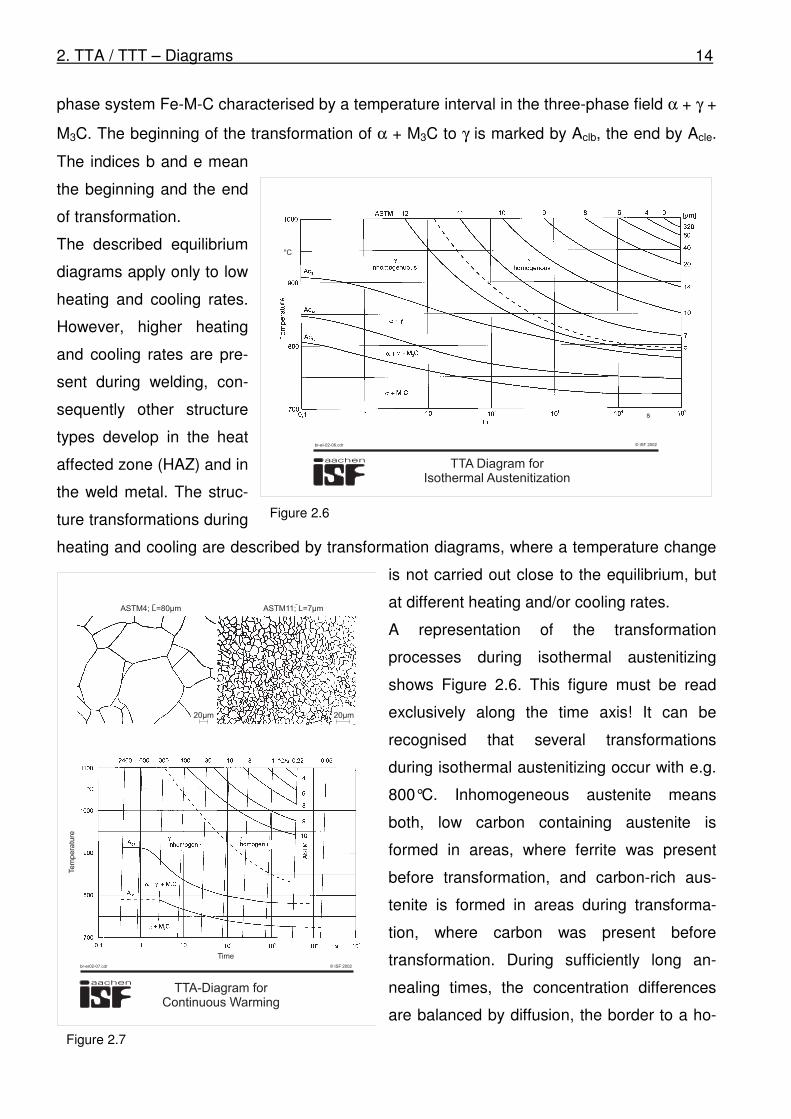
The influence of heating rate on austenitizing is shown in Figure 2.7. This diagram must only

be read along the sloping lines of the same heating rate. For better readability, a time pattern

was added to the pattern of the heating curves. To elucidate the grain coarsening during aus-

tenitizing, two microstructure photographs are shown, both with different grain size classes to

ASTM.

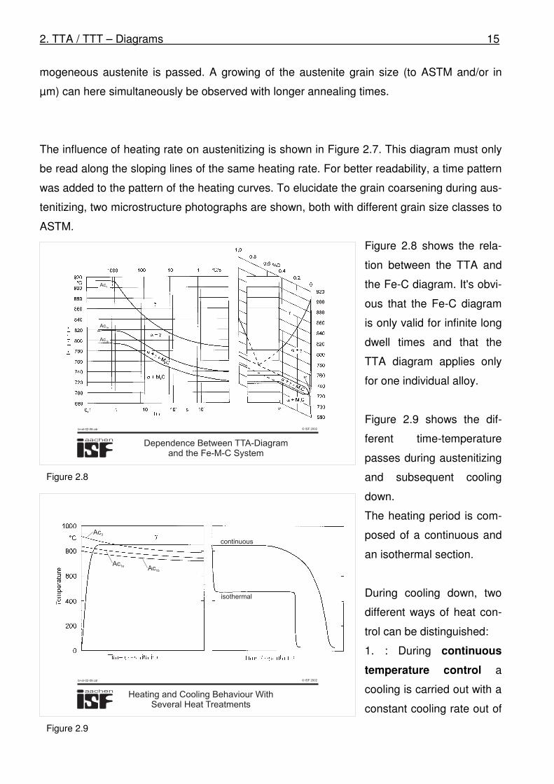
Figure 2.8 shows the rela-

tion between the TTA and

the Fe-C diagram. It's obvi-

ous that the Fe-C diagram

is only valid for infinite long

dwell times and that the

TTA diagram applies only

for one individual alloy.

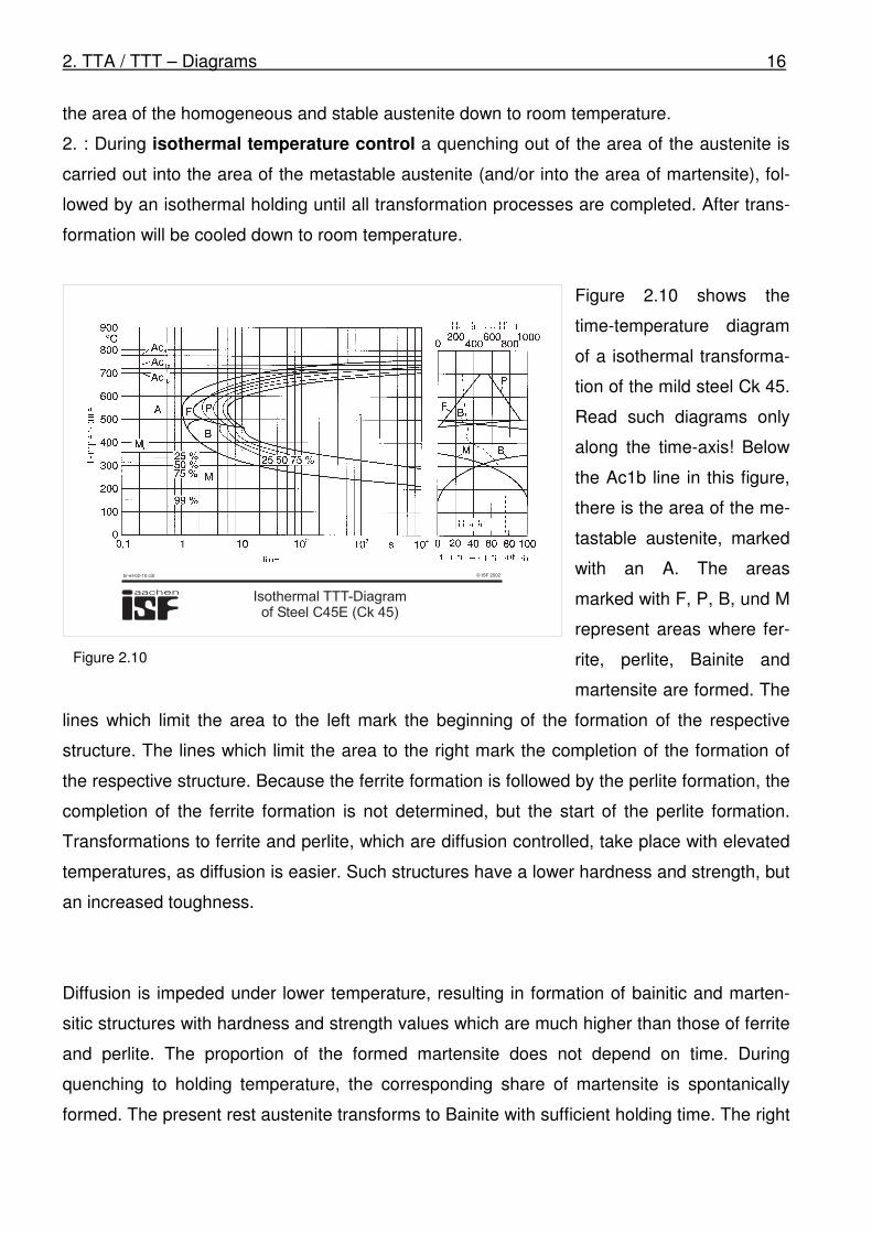
Figure 2.9 shows the dif-

ferent time-temperature

passes during austenitizing

and subsequent cooling

down.

The heating period is com-

posed of a continuous and

an isothermal section.

During cooling down, two

different ways of heat con-

trol can be distinguished:

1. : During continuous

temperature control a

cooling is carried out with a

constant cooling rate out of

Dependence Between TTA-Diagramand the Fe-M-C System

Ac3

Ac1e

Ac1b


Figure 2.8

Heating and Cooling Behaviour WithSeveral Heat Treatments

Ac3

Ac1e Ac1b

continuous

isothermal


Figure 2.9


the area of the homogeneous and stable austenite down to room temperature.

2. : During isothermal temperature control a quenching out of the area of the austenite is

carried out into the area of the metastable austenite (and/or into the area of martensite), fol-

lowed by an isothermal holding until all transformation processes are completed. After trans-

formation will be cooled down to room temperature.

Figure 2.10 shows the

time-temperature diagram

of a isothermal transforma-

tion of the mild steel Ck 45.

Read such diagrams only

along the time-axis! Below

the Ac1b line in this figure,

there is the area of the me-

tastable austenite, marked

with an A. The areas

marked with F, P, B, und M

represent areas where fer-

rite, perlite, Bainite and

martensite are formed. The

lines which limit the area to the left mark the beginning of the formation of the respective

structure. The lines which limit the area to the right mark the completion of the formation of

the respective structure. Because the ferrite formation is followed by the perlite formation, the

completion of the ferrite formation is not determined, but the start of the perlite formation.

Transformations to ferrite and perlite, which are diffusion controlled, take place with elevated

temperatures, as diffusion is easier. Such structures have a lower hardness and strength, but

an increased toughness.

Diffusion is impeded under lower temperature, resulting in formation of bainitic and marten-

sitic structures with hardness and strength values which are much higher than those of ferrite

and perlite. The proportion of the formed martensite does not depend on time. During

quenching to holding temperature, the corresponding share of martensite is spontanically

formed. The present rest austenite transforms to Bainite with sufficient holding time. The right

Isothermal TTT-Diagramof Steel C45E (Ck 45)


Figure 2.10


detail of the figure shows the present structure components after completed transformation

and the resulting hardness at room temperature.

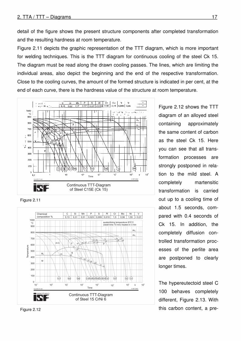
Figure 2.11 depicts the graphic representation of the TTT diagram, which is more important

for welding techniques. This is the TTT diagram for continuous cooling of the steel Ck 15.

The diagram must be read along the drawn cooling passes. The lines, which are limiting the

individual areas, also depict the beginning and the end of the respective transformation.

Close to the cooling curves, the amount of the formed structure is indicated in per cent, at the

end of each curve, there is the hardness value of the structure at room temperature.

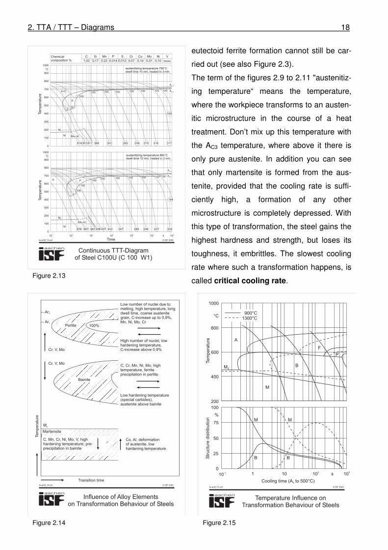
Figure 2.12 shows the TTT

diagram of an alloyed steel

containing approximately

the same content of carbon

as the steel Ck 15. Here

you can see that all trans-

formation processes are

strongly postponed in rela-

tion to the mild steel. A

completely martensitic

transformation is carried

out up to a cooling time of

about 1.5 seconds, com-

pared with 0.4 seconds of

Ck 15. In addition, the

completely diffusion con-

trolled transformation proc-

esses of the perlite area

are postponed to clearly

longer times.

The hypereutectoid steel C

100 behaves completely

different, Figure 2.13. With

this carbon content, a pre-

Continuous TTT-Diagramof Steel C15E (Ck 15)

Time

27

40

19

370 235 220 170


Figure 2.11

MS

M

A+C F

B

5

5522

P

25

2

23

Ac3

Ac1

Chemicalcomposition %

SiC Mn P S Al Cr Mo Ni V

0,13 0,31 0,51 0,023 0,009 0,010 1,5 0,06 1,55 < 0,01

10-1

100

101

102

103

104 10

510

6

0

100

200

300

400

500

600

700

800

900

1000

s

°C

Tem

pera

ture

Time

austenitizing temperature 870°C(dwell time 10 min) heated in 3 min

25

4767

7510

75 7525

257575

60

7255

3730

22

9

417 400 396 314 304 287 268 251 224 192 167 152 151

Continuous TTT-Diagramof Steel 15 CrNi 6


Figure 2.12


eutectoid ferrite formation cannot still be car-

ried out (see also Figure 2.3).

The term of the figures 2.9 to 2.11 "austenitiz-

ing temperature“ means the temperature,

where the workpiece transforms to an austen-

itic microstructure in the course of a heat

treatment. Don’t mix up this temperature with

the AC3 temperature, where above it there is

only pure austenite. In addition you can see

that only martensite is formed from the aus-

tenite, provided that the cooling rate is suffi-

ciently high, a formation of any other

microstructure is completely depressed. With

this type of transformation, the steel gains the

highest hardness and strength, but loses its

toughness, it embrittles. The slowest cooling

rate where such a transformation happens, is

called critical cooling rate.

0

100

200

300

400

500

600

700

800

900

1000

°C

Tem

pera

ture

10-1

100

101

102

103

104

105

0

100

200

300

400

500

600

700

800

900

1000

s

°C

Te

mp

era

ture

Time

P

2 15

100

100 100 100 100 100 100

AC1e

AC1b100

MS

M RA 30»

914 901 817 366 351 283 236 215 214 177

180

A+C

AC1e

AC1b

MS

M

A P

C

100100

100

1005

100 100 100 100 100

RA 0»4

876 887 867 496 457 442 347 289 246 227 200

194

Continuous TTT-Diagramof Steel C100U (C 100 W1)


Mn P S Cr Cu Mo Ni V

1,03 0,17 0,22 0,014 0,012 0,07 0,14 0,01 0,10 traces

C Si

austenitizing temperature 790°Cdwell time 10 min, heated in 3 min

austenitizing temperature 860°Cdwell time 10 min, heated in 3 min


Figure 2.13

Influence of Alloy Elementson Transformation Behaviour of Steels

Tem

pera

ture

Transition time

Low number of nuclei due tomelting, high temperature, longdwell time, coarse austenitegrain, C-increase up to 0,9%,Mn, Ni, Mo, Cr

High number of nuclei, lowhardening temperature,C-increase above 0,9%

Ar1

Ar3

Perlite 100%

Cr, V, Mo

Cr, V, Mo

Bainite

C, Cr, Mn, Ni, Mo, hightemperature, ferriteprecipitation in perlite

Low hardening temperature(special carbides),austenite above bainite

C, Mn, Cr, Ni, Mo, V, highhardening temperature, pre-precipitation in bainite

Martensite

Co, Al, deformationof austenite, lowhardening temperature

Ms


Figure 2.14

Temperature Influence onTransformation Behaviour of Steels

Te

mp

era

ture

1000

800

A

600

400

200

°C

MS

M

B

F

P

900°C1300°C

Str

uctu

re d

istr

ibu

tio

n

100

75

50

25

0

%M M

B B

10-1 1 10 10

210

3s

Cooling time (A to 500°C)3


Figure 2.15


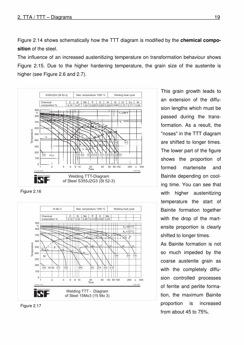
Figure 2.14 shows schematically how the TTT diagram is modified by the chemical compo-

sition of the steel.

The influence of an increased austenitizing temperature on transformation behaviour shows

Figure 2.15. Due to the higher hardening temperature, the grain size of the austenite is

higher (see Figure 2.6 and 2.7).

This grain growth leads to

an extension of the diffu-

sion lengths which must be

passed during the trans-

formation. As a result, the

"noses" in the TTT diagram

are shifted to longer times.

The lower part of the figure

shows the proportion of

formed martensite and

Bainite depending on cool-

ing time. You can see that

with higher austenitizing

temperature the start of

Bainite formation together

with the drop of the mart-

ensite proportion is clearly

shifted to longer times.

As Bainite formation is not

so much impeded by the

coarse austenite grain as

with the completely diffu-

sion controlled processes

of ferrite and perlite forma-

tion, the maximum Bainite

proportion is increased

from about 45 to 75%.

Welding TTT-Diagramof Steel S355J2G3 (St 52-3)

0

100

200

300

400

500

600

700

800

900

1 2 4 6 8 10 20 40 60 80 100 200 400sTime

Te

mp

era

ture

449 420 400 363 334 324 270 253 251 249

222 215

243

°C


SiC Mn P S Al N Cr Cu Ni

0,16 0,47 1,24 0,029 0,029 0,024 0,0085 0,10 0,17 0,06

Max. temperature 1350 °C Welding heat cycle

48

75

S355J2G3 (St 52-3)

55


B

Figure 2.16

Welding TTT - Diagramof Steel 15Mo3 (15 Mo 3)

0

100

200

300

400

500

600

700

800

900

°C

1 2 4 6 8 10 20 40 60 80 100 200 400sTime

Tem

pera

ture

440 431 338 285 255 234 224 210

208 200 178

A =861°Cc3

A =727°Cc1

MS

B

F

HV30

P

M

14 7487

95

99 83 77 60 38 15

1 7 19 4 8

32 45

17

53

32


SiC Mn P S Mo

0,16 0,30 0,68 0,012 0,038 0,29

15 Mo 3 Max. temperature 1350 °C Welding heat cycle


Figure 2.17


Due to the strong influence of the austenitizing temperature to the transformation behaviour

of steel, the welding technique uses special diagrams, the so called Welding-TTT-diagrams.

They are recorded following the welding temperature cycle with both, higher austenitizing

temperatures (basically between 950° and 1350°C) and shorter austenitizing times.

You find two examples in Figures 2.16 and 2.17.

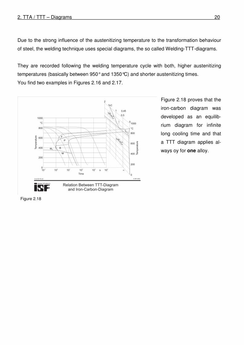
Figure 2.18 proves that the

iron-carbon diagram was

developed as an equilib-

rium diagram for infinite

long cooling time and that

a TTT diagram applies al-

ways oy for one alloy.

Relation Between TTT-Diagramand Iron-Carbon-Diagram

F

P

0

200

400

600

800

°C

1000

10-1

100

101

102

103

104

s ¥

B

M

0

200

400

600

800

°C

10000

0,451

%C

2

MSTe

mp

era

ture

Te

mp

era

ture

Time

0,5


Figure 2.18

2. TTA / TTT - Diagrams - KAUmercury.kau.ac.kr/welding/Welding Technology II - Welding... · 2. TTA...

Documents

Transcript of 2. TTA / TTT - Diagrams - KAUmercury.kau.ac.kr/welding/Welding Technology II - Welding... · 2. TTA...