Phase Diagrams and Cluster Expansions for Low...
44
Communications in Commun. Math. Phys. 82, 261-304 (1981) Mathematical Physics © Springer-Verlag 1981 Phase Diagrams and Cluster Expansions for Low Temperature @ > (φ) 2 Models* I. The Phase Diagram JohnZ. Imbrie*** Department of Physics, Harvard University, Cambridge, MA 02138, USA Abstract. Low temperature phase diagrams of two-dimensional 0*(φ) quantum field models are constructed. Let 3P lie in an (r— l)-dimensional space of perturbations of a polynomial with r degenerate minima. Perform a scaling and assume λ<ζl. We construct k distinct states on . . hypersurfaces of codimension k— 1 in the space of perturbations. An expansion is used to exhibit exponential clustering of the Schwinger functions of each of these states. At the core of the construction is a general technique for finding the thermodynamically stable phases from a collection of competing minima. We draw on ideas of Pirogov and Sinai [24] for this problem. Table of Contents Part I. The Phase Diagram 1. Introduction .................................. 262 1.1. Background and Main Results ........................ 262 1.2. Physical Ideas and Outline ................ . ......... 265 2. Mean Field Expansion ............ .................. 267 2.1. Polynomials and the A->0 Limit ........... . ............ 267 2.2. Expansion in Phase Boundaries ........................ 270 2.3. Translation of ψ q . . ........... . ................ 271 2.4. Decoupling Expansion and Mass Shifts ..................... 273 2.5. Estimates Needed in Chaps. 3 and 4 ...................... 279 3. The Search for Stable Phases : Ratios of Partition Functions .............. 281 3.1. The Physics : Surface Energies and Collapsing Expansions ............. 281 3.2. Contour Models ............................... 284 3.3. Expansions for the Pressure and Surface Energy ................. 285 3.4. Contour Models with Parameters : An Inductive Construction ........... 288 3.5. An Equation that Yields the Ratio of Partition Function Estimate ......... 297 3.6. Solving L = ^(L) by Iteration ......................... 298 3.7. The Phase Diagram ............................. 301 * Supported in part by the National Science Foundation under Grant No. PHY-79-16812 ** National Science Foundation predoctoral fellow, 1979-1980. Currently Junior Fellow, Harvard University Society of Fellows 0010-3616/81/0082/0261/S08.80
Transcript of Phase Diagrams and Cluster Expansions for Low...
Communications inCommun. Math. Phys. 82, 261-304 (1981) Mathematical
Physics© Springer-Verlag 1981
Phase Diagrams and Cluster Expansionsfor Low Temperature @>(φ)2 Models*
I. The Phase Diagram
JohnZ. Imbrie***
Department of Physics, Harvard University, Cambridge, MA 02138, USA
Abstract. Low temperature phase diagrams of two-dimensional 0*(φ) quantumfield models are constructed. Let 3P lie in an (r— l)-dimensional space ofperturbations of a polynomial with r degenerate minima. Perform a scaling
and assume λ<ζl. We construct k distinct states on ..
hypersurfaces of codimension k— 1 in the space of perturbations. An expansionis used to exhibit exponential clustering of the Schwinger functions of each ofthese states. At the core of the construction is a general technique for findingthe thermodynamically stable phases from a collection of competing minima.We draw on ideas of Pirogov and Sinai [24] for this problem.
Table of Contents
Part I. The Phase Diagram
1. Introduction .................................. 2621.1. Background and Main Results ........................ 2621.2. Physical Ideas and Outline ................ . ......... 265
2. Mean Field Expansion ............ .................. 2672.1. Polynomials and the A->0 Limit ........... . ............ 2672.2. Expansion in Phase Boundaries ........................ 2702.3. Translation of ψq . . ........... . ................ 2712.4. Decoupling Expansion and Mass Shifts ..................... 2732.5. Estimates Needed in Chaps. 3 and 4 ...................... 279
3. The Search for Stable Phases : Ratios of Partition Functions .............. 2813.1. The Physics : Surface Energies and Collapsing Expansions ............. 2813.2. Contour Models ............................... 2843.3. Expansions for the Pressure and Surface Energy ................. 2853.4. Contour Models with Parameters : An Inductive Construction ........... 2883.5. An Equation that Yields the Ratio of Partition Function Estimate ......... 2973.6. Solving L = ̂ (L) by Iteration ......................... 2983.7. The Phase Diagram ............................. 301
* Supported in part by the National Science Foundation under Grant No. PHY-79-16812** National Science Foundation predoctoral fellow, 1979-1980. Currently Junior Fellow, HarvardUniversity Society of Fellows
0010-3616/81/0082/0261/S08.80
262 J. Z. Imbrie
Part II. The Schwinger Functions
4. An Expansion for the Schwinger Functions 3054.1. Constrained Expansions 3054.2. More General Ratios of Partition Functions 3064.3. Exponential Clustering and Asymptoticity of the Perturbation Series 3094.4. The Convergence Lemmas 317
5. Convergence Estimates 3205.1. Structure of the Estimates 3205.2. Wick Ordering Lower Bounds 3215.3. Vacuum Energy Bounds 3245.4. Lower Bounds for ZΔm and ZΣ 3295.5. Estimates on Mass Shift Normalization Factors 3315.6. Decoupling Expansion Estimates 3345.7. The Bounded Spin Approximation 3385.8. Smoothness in μ 341
I. Introduction
ί .1. Background and Main Results
This paper presents a detailed analysis of low-temperature 0>(φ)2 quantum fieldsmodels. The last several years have seen considerable development of constructivefield theory techniques for studying multiphase models. However, the range ofmodels that can be treated remains rather limited when compared with the largeclass of polynomials to which expansion techniques ought to apply. We close thisgap by giving cluster expansions for the Schwinger functions of essentiallyarbitrary low-temperature έP(φ)2 models. Moreover, we construct coexisting stateson various hypersurfaces of a phase diagram homeomorphic to the classical (zerocoupling) phase diagram. A unique feature of this investigation is the fundamentalrole expansions play in determining the stable phases of a theory.
The study of phase transitions in quantum fields models was initiated byGlimm, Jaffe and Spencer [18] with their proof that two phases exist in thedouble-well (λφ4 — ̂ φ2)2 model. Subsequent results include existence of phasetransitions for models without a symmetry [9] or with continuous symmetry[11,12], and absence of symmetry breakdown for vector models in twodimensions [2].
Gaw^dzki [13] proved that the parameters in a φ6 polynomial can be adjustedso as to achieve three distinct phases at one point. Summers [28,29] establishedthat two phases coexist on lines leading up to that point. These results justifiedclassical ideas about the structure of the phase diagram of that model.
Of course, there are a number of methods available to construct modelscorresponding to general polynomials [14,10]. But these methods do not leaddirectly to results on multiplicity of phases or phase transitions.
When dealing with a model that is a small perturbation of a massive Gaussian,cluster expansions usually give the most detailed information, e.g. on the relationbetween the Schwinger functions and their perturbation series [6,8] or on clusterproperties [16,17]. This has been the case for multiphase theories also. Glimm etal. [19] developed a convergent expansion for the Schwinger functions of the
model (with |μ|^A2<^l), establishing also the mass gap of the
Phase Diagrams. I 263
theory. Their mean field expansion has formed a basis for studies of other modelswith deep, widely separated minima. The technique was used for the Coulomb gas[3,4], for a two-component φ4 model with three phases [5], and for thepseudoscalar Yukawa model in the two-phase region [1]. Summers [28] used it inthe φ6 model mentioned above, although his expansion did not converge in aneighborhood of the asymmetric phase transition lines. (He was nevertheless ableto prove asymptoticity of perturbation theory across the phase transitionlines [30].)
The work cited above goes very far in the description of quantum fields at ornear first-order phase transitions. However, all the results depend in an essentialway on special properties of the models considered. In all of the models, the spaceof parameters in the interaction has an a priori reduction to 0 or 1 dimensions withthe use of symmetries or correlation inequalities. Thus all work has depended oneither
(i) the existence of a preferred point in parameter space at which the phasetransition should occur (e.g., a symmetric point) or
(ii) the existence of a preferred direction in parameter space along which onecan pass to obtain the phase transition.
The Glimm-Jaffe-Spencer analysis of (λφ4 — ̂ φ2 — μφ)2 [19], and Frohlich'sproof of phase transitions without symmetry breaking [9] rely on the external fieldas the preferred direction. Gaw^dzki's proof of the existence of three phases [13]uses both (i) and (ii): a φ-^ — φ symmetry prevailed all along the direction ofvariation of a quadratic term in the polynomial. Summers's analysis of the phasediagram of that model [28,29] also used the quadratic coefficient as the preferreddirection, even though the diagram was two-dimensional. Baίaban andGaw^dzki's work on the two-phase Yukawa model [1] used a boson symmetryφ-+ — φ. Brydges and Federbush [3,4] and Constantinescu and Ruck [5] alsoused symmetries in their multiphase expansions.
The limitations (i) and (ii) rule out a wide range of situations where one expectsphase transitions. A general polynomial will have many local minima. Theprocess of adjusting the coefficients of the polynomial to achieve many phases atonce involves many parameters nontrivially. One of the main contributions of thispaper is a technique for finding the hypersurfaces on which various phases of apolynomial coexist. If r phases are involved, this involves a search through an(r— l)-dimensional space of parameters, with no preferred directions and nosymmetries.
We also obtain detailed properties of each of the phases by giving a clusterexpansion which converges throughout the space of parameters. This represents aconsiderable advance in expansion techniques, since up till now all clusterexpansions have relied on symmetries [19,3-5,1], correlation inequalities[19,20,28], or large differences in classical energy densities [28]. When correlationinequalities are used, one is in case (ii) above. A large difference in classical energydensities necessarily excludes neighborhoods of phase transition hypersurfacesfrom consideration.
The main difficulty with applying expansion techniques to general polynomialshas been in obtaining ratio of partition function bounds. These bounds areabsolutely crucial in getting the boundary conditions to select a stable phase.
264 J. Z. Imbrie
Except in situations (i) and (ii) above, it is not clear which minima are stable andwhich ones are unstable at a particular choice of parameters. Quantum fluc-tuations can suppress some minima relative to others, making the classicalpolynomial an unreliable guide. One can only hope to obtain good bounds onratios of partition functions when a stable partition function is in the denominator.Thus the difficulty is compounded by the fact that one does not know which ratiosof partition functions one should attempt to bound.
This problem has been solved in lattice statistical mechanics where spins takevalues in a finite set. Pirogov and Sinai [23,24] have developed a powerfultechnique to give a complete analysis of the phase diagrams of such models at lowtemperatures. They show that in the (r — l)-dimensional space of perturbations of a
MHamiltonian with r degenerate ground states, there exist hypersurfaces ofcodimension k— 1 at which k phases coexist. ^ '
We solve the ratio of partition function problem by drawing on the ideas ofPirogov and Sinai. Quantum field models, and unbounded spin systems in general,have a number of properties which make a straightforward application of thePirogov-Sinai theory impossible. The difficulties arise from the nonpositivity ofterms of the decoupling expansion, from different classical masses in differentminima, and from the unboundedness of φ. These will be discussed in the nextsection, and as they arise in later chapters.
The techniques of this paper should also be useful in solving problems outsideof 0*(φ)2 theory. At no point do we use symmetries or correlation inequalities toobtain the expansion. The techniques should apply to the low temperaturestatistical mechanics of continuous, unbounded spins (not covered in [23,24]).They may be applicable to the problem of proving Debye screening for arbitraryrelative activities of charge species. (See [4] for a statement of this problem.)
We now state the main results. Let μ vary in some neighborhood of the originin R1""1. Let &Ίtμ(ξ) be a polynomial with local minima at ξ = ξl(μ)9 ...9ξr(μ).Suppose these minima are degenerate when μ=0, and suppose 0>fί,μ(ζq) = mq(μ)>Qfor q = l9...9r. Assume ^ μ is bounded below and its minima ξί9...9ζr areseparated by potential barriers. We give a more precise statement of therequirements on ^\ μ in Sect. 2.1. The parameters μl must break the degeneracyproperly, and the classical energies ̂ μ(ξq\ cannot be too far apart.
With
0>λitι(ξ) = λ-20>lfμ(λξ)9 (1.1.1)
we construct finite volume expectations as follows. Define
Vq=ϊ\ P* ,(</>(*)) -*Vμ(£«)- ̂ :(ΦM~Q2'•}a*Λl * J
where ψq(x) = φ(x) — ξq. Wick ordering is defined with respect to the covariance( —zl+ml)"1, where qe{l9...9r} is fixed throughout. Let dμm2(ψq) denote theGaussian measure in which ψq has mean zero and covariance ( — A +mq)~1. The
Phase Diagrams. I 265
expectation with boundary condition q is
m2
The measure dμm%(ψq) supplies the missing mass term -~:ψq(x)2: in Λ, while
outside A it forces the field to lie near the qth minimum. The scaling (1.1.1)preserves the shape of 0*ίtμ, while separating the minima by factors of λ~1 andraising potential barriers by factors of λ~2. Quadratic terms are unaffected, whilecubic and higher coefficients are multiplied by powers of λ.
Theorem 1.1.1. Let λ be sufficiently small. There exists a Lipschitz continuousmapping of a neighborhood of the origin in parameter space onto a neighborhoodof the origin in the boundary of the positive octant in JRr. I This is the set of r-tuples
(α1, ...,</) satisfying infα^=0.j The mapping inverts and the inverse is also
Lipschitz continuous. Let μ be a parameter set which is the inverse image of a pointwith aq = Q. At μ, the infinite volume limit of the Schwinger functions
Π Φ(xj) (1-1.4)i = l /Λ,q
exists and the limiting functions satisfy all the Osterwalder-Schrader axioms [22]with exponential clustering.
The perturbation series for the qth-state Schwinger functions are asymptotic as(Λ
λ-+Q whenever aq(μ) = Q. As a consequence there exist hypersurfaces ofwcodimension k — 1 in parameter space at which k distinct phases coexist.
In the course of proving this theorem we give rather precise estimates on thepositions of the phase transition hypersurfaces. In Sect. 3.7 it is shown that theydeviate by 0(λ512) from the positions inferred from perturbation theory throughorder λ° for the vacuum energies.
This paper incorporates and extends the author's doctoral thesis [21], wherethe central ideas were worked out in a less general setting.
1.2. Physical Ideas and Outline
In this section we present some of the main ideas behind the proof ofTheorem 1.1.1. An organizational overview will be given at the same time. Moredetailed discussions and analyses of technical problems will be found at thebeginnings of Chaps. 3-5.
Chapter 2 gives a version of the mean field expansion that is suited to variablemass polynomials and to the constructions in Chap. 3. The basic objects used inthe rest of the paper are defined, and estimates on them are stated in Sect. 2.5. InSect. 2.1 we give a precise statement of requirements on polynomials, and we singleout aspects that ultimately determine how small λ must be taken. A concisestatement of the choice of constants used in the expansions is also given inSect. 2.1.
266 J. Z. Imbrie
The basic idea of the mean field expansion is to decompose the theory into low-and high-momentum modes. The low-momentum part resembles a lattice spinsystem; it is controlled with a Peierls expansion. The high-momentum partresembles a single-phase model it is controlled with a decoupling expansion in thespirit of [17]. The low-momentum component (the "mean field") is defined byaveraging the field over a square. Rigorous bounds on the deviation of the fieldfrom its average value justify the splitting and provide a basis for the vacuumenergy bounds.
The mean field expansion expresses the theory in terms of a statistical ensembleof objects defined on finite regions of IR2. (Actually, it is not a true statisticalensemble because the objects are not in general positive.) This is the starting pointfor the analysis of Chap. 3.
In Chap. 3 the stable phases are determined and the all-important ratio ofpartition function bounds are established. We use many of the ideas of Pirogovand Sinai [23,24], though the constructions we give are quite different fromanalogous ones in [24]. We emphasize partition function language over thecontour language of [23,24]. We must avoid taking logarithms of the basicobjects, since there is no way to keep them positive and bounded away from zero.
The constructions proceed through approximations to quantities representingthe "relative energies" of the different phases. For each set of approximate energies,approximate partition functions are constructed. The physical basis of theconstruction is the idea that transitions out of an unstable phase should have aprobability growing exponentially with the volume of the fluctuation. Thecoefficient should be proportional to the energy of the phase relative to the stablephases. In contrast to the true partition functions, the approximate partitionfunctions can be estimated at this stage.
Estimating approximate partition functions is the technical crux of this work.The estimate depends on the fact that there is a form in which the expansion haspositive terms. In order to be able to reduce to that form at any point, we must usea complicated inductively defined construction for the approximate partitionfunctions. The "relative energies" acquire a dependence on the size of fluctuations.
The approximate partition functions are estimated in terms of pressures andsurface energies. The pressure terms correct the approximate relative energies, andthe surface terms are incorporated into the ensemble. This new information yieldsa better approximation to the partition function, and the procedure repeats. Whenthe iteration converges, we have expansions for the true partition functions. Thestable phases are the ones with zero relative energy. The estimate mentioned abovecan be applied to give good bounds on ratios of partition functions, provided astable phase is in the denominator.
In Chap. 4 the information on partition function is used to obtain anexpansion for the Schwinger functions. Ratios of constrained partition functionsmust be dealt with before dispensing with the machinery of Chap. 3. Constraintson the expansion for J RQ~Vqdμm2(ψq) can be handled with some techniques of Kunzand Souillard (see [1]), and the normalization §e~~Vqdμm2(ψq) can be factored outexplicitly. This yields estimates on (RyΛ)q independent of Λ9 for q a stable phase.Other consequences of the convergence of the expansion are the mass gap and theasymptotic nature of perturbation theory.
Phase Diagrams. I 267
Chapter 5 contains proofs of the estimates required for Chaps. 3 and 4. It isessential to take account of the effective vacuum energy arising from changes inmass. We also require some smoothness in μ for each element of the expansion. Toobtain smoothness of partition functions associated with a single spin con-figuration, we need a new type of estimate approximating the field as a boundedspin. This estimate is what allows us to go beyond [21] to give a complete pictureof the phase diagram.
2. Mean Field Expansion
2.1. Polynomials and the λ-+Q Limit
In this section we specify precisely the polynomials and perturbations that will betreated in this paper. Our philosophy will be to specify a polynomial ̂ and thenscale ̂ and its argument according to
0>λ(ξ) = λ-2&ί(λξ), λe(0,l]. (2.1.1)
This scaling has the effect of separating minima by λ~l and increasing barriersbetween minima by λ~2. The curvatures at the minima of 3Pλ are independent of A.The coupling constant λ can be identified with h1/2, so that as λ tends to zero weapproach the classical limit. Alternatively, we can think of the scaling as acontinuum version of the low temperature limit for the lattice Hamiltonian# = f I F0I2 + ̂ χ (0). With λ = β~1/2, j8>l, the change of variable φ-+λφ sends βH
The scaling is particularly useful in studying ^(φ)2 theories that possess manyphases, because it preserves whatever multiple-well structure ^ has. In thisrespect it differs from λ^(φ) — φ2, λ<ζl and g&(φ\ 0>1, which should yield onlyone- or two-phase theories [25].
We shall give a convergent r-phase expansion for the Schwinger functionswhen λ <^ 1 and &λ has r important minima. (The meaning of "important" will bespecified precisely below.) As parameters in έPλ are varied, a minimum may rise sofar above the others that it becomes irrelevant. If this happens, we are able to giveoverlapping r-phase and (r— l)-phase expansions. Thus we can handle generalpolynomials except in neighborhoods of critical points.
In order to achieve coexistence of up to r-phases, we need to considerperturbations of polynomials with r degenerate minima. Quantum corrections willdestroy the degeneracy, and we must be able to restore it by making small changesin the perturbing parameters. Let μ = (μ1, ...,μr~1). We take &*ί=0*ίfμ andsuppose that ̂ 0 has r degenerate minima.
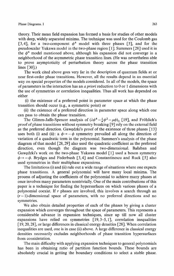
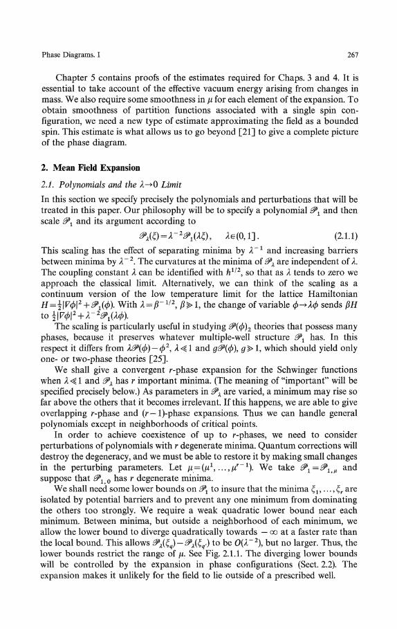
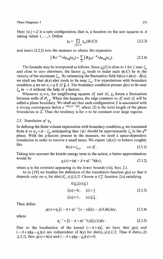
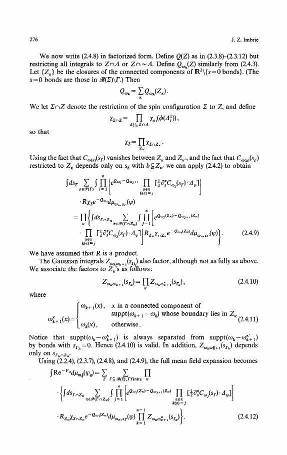
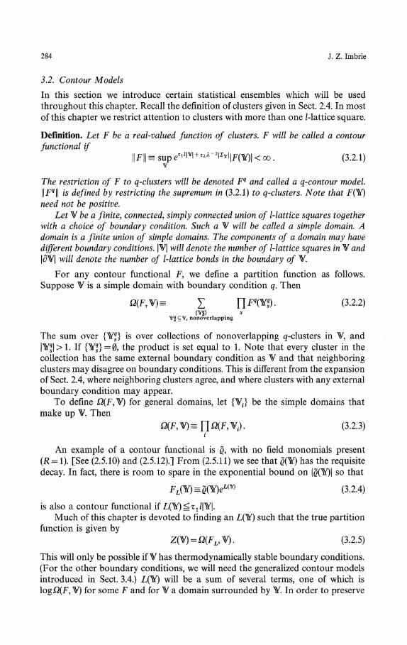
We shall need some lower bounds on ̂ to insure that the minima ξl9...9ξr areisolated by potential barriers and to prevent any one minimum from dominatingthe others too strongly. We require a weak quadratic lower bound near eachminimum. Between minima, but outside a neighborhood of each minimum, weallow the lower bound to diverge quadratically towards — oo at a faster rate thanthe local bound/This allows ^λ(ξq)-^λ(ξq') to be 0(λ~2\ but no larger. Thus, thelower bounds restrict the range of μ. See Fig. 2.1.1. The diverging lower boundswill be controlled by the expansion in phase configurations (Sect. 2.2). Theexpansion makes it unlikely for the field to lie outside of a prescribed well.
268 J. Z. Imbrie
P ( g )
Fig. 2.1.1. Lower bounds required of 0*(ξ). ζ is fixed, while f? ̂ ζ/4 may be taken to be small. However,
We now give a precise statement of the requirements on ^\ μ and^l, μ), . . . , ξr(l, μ). { l̂f μ, ξl9..., ξr} will be called C^C-admissible if for all' μ. with
(i) ξl9..., ξr are local minima of <β.
(in) Define d and ajΛ(μ) by the formula
d\ vi = > n,.' *—* j» <
Then rf is even, d^C, \ad q(μ)\^C~\ and \a} q(μ)\^C, j^2. Of course βj 4(μ)=0.Write α2ι» = i
(iv) ξ^i-(v) There is a #e{l, ...,r} such that eq = Eq
c — E* satisfies the followingίdeq\
condition. If A is an eigenvalue of the matrix l^-Lφ- , then |vl|e[C 1
9 C].
(vi)d2eq
^brflA. ^ C, and6μidμ
(vii)Put ξ0=-oo, ξr+ί = co.For q = l, ...,r,
_ (̂ c^ ^ > ^/ ^l,μV<V =
Phase Diagrams. I 269
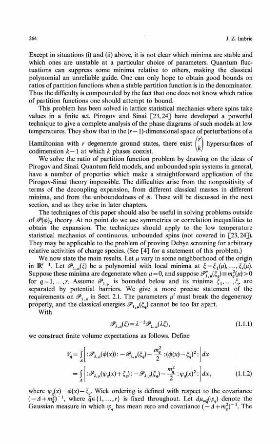
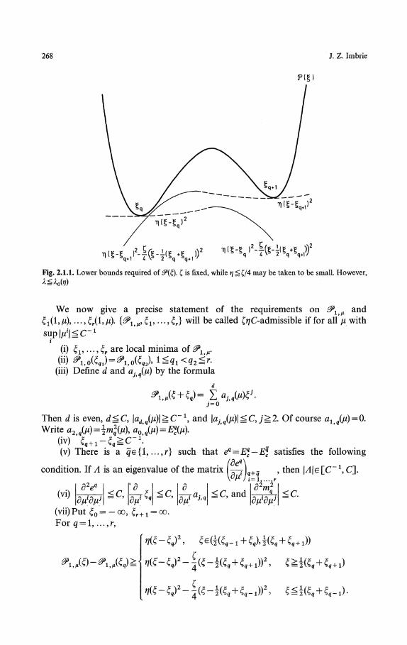
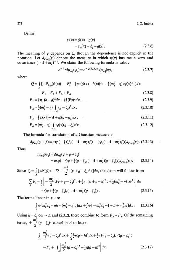
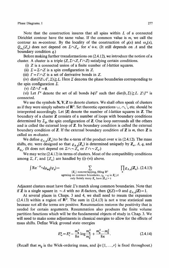
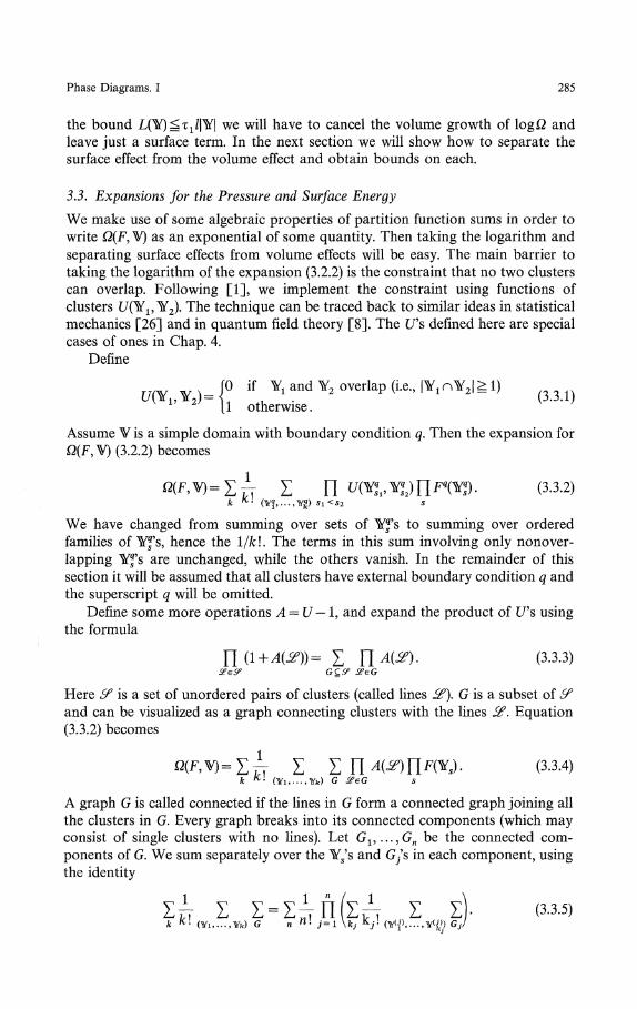
Fig. 2.1.2. If η is decreased fromconsideration
to η2, then the right-hand minimum can be omitted from
The constants ζ, η, and C that appear in the above definition arise as follows, ζis a constant chosen consistently with some upper limits arising in the proof of thevacuum energy bound (Sects. 5.2 and 5.3). η may be chosen at will in the range(0>£/4] However, the lower bounds (vii) allow for a reasonable range ofperturbations μ only if η is a small fraction of ζ. Also, the lower bounds imply thatwiq ̂ 2τ/ for all q. As η tends toward zero, we must restrict λ to smaller ranges. Byadjusting η, one can exclude a minimum from consideration in a restricted range ofμ (Fig. 2.1.2). Thus the domains of convergence of expansions with different valuesof r overlap. The constant C parametrizes various aspects of the polynomial whichultimately will affect the maximum allowable λ. Thus C and η~l may be chosenarbitrarily large, but we require λ<λQ(η,C).
Requirement (v) insures that the parameters μ1 break the degeneracy of ̂ 0
and establishes a scale for μ1. With E*(λ, μ) — &λ>μ(ζq\ we have that a change δμ inthe parameters induces a change δEq
c = O(λ~2)δμ in the classical energies of theminima. Requirement (vi) is used to prove convergence of successive approxi-mations to phase coexistence points. We need (v) and (vi) only in Sect. 3.7, wherecoexistence is established.
The ^-derivatives of the aj>qs can be expressed as nonsingular rationalfunctions of μ-derivatives of the coefficients of &. (Singularities appear only whensome mq tends to zero.)
The bound ξq+1 — ξq ̂ C~1 orders the minima and helps to avoid any potentialcritical points. Together with the lower bounds (vii), it insures that fluctuationsbetween minima incur a certain energetic cost. The minima of 0*λtfl are at ξq(λ)= λ'1ξq (λ=ί). Thus they are separated by 0(λ~*).
Two length scales will be used in constructing the mean field expansion. One isthe scale on which distant regions are decoupled in the cluster expansion.Decoupling lines are placed on a lattice with squares of length /. We choose I to bea large integer, depending on C and η. I need not diverge with λ. However, λ must
270 J. Z. Imbrie
be chosen sufficiently small, depending on /. The qualification λ <ζ 1 <^ I will alwaysrefer to this choice of constants. Once λ and / are chosen as described above, all ourresults apply to any Cf/C-admissible family of polynomials. A second length Lprovides an upper bound on the scale of effects of fluctuations between minima.We take L to be the next multiple of / after (log/I)2.
More general polynomials can be brought into Cf/C-admissible form byperforming two operations. A dilation ^->e>2^, x-+δ~ 1x can be used to bring the
masses into the range [ j/2τ/, |/2C] or to increase the range of parametersconsistent with the lower bounds (vii). A preliminary scaling 0>(φ)-+y~2έP(yφ) willleave the masses fixed while bringing the leading coefficient into the range
2.2. Expansion in Phase Boundaries
In the next three sections we present the mean field expansion [19] that we will usethroughout this paper. It consists of four parts : an expansion in phase boundaries,a translation of the field, decoupling expansions, and mass shifts. The last twooperations are intertwined in a way that generates an expansion with the rightlocality properties. Shifts of mass from the measure to the interaction or vice versaare needed so that the decoupling expansion is always controlled by factors of λ.These multiply cubic and higher order terms in the interaction, but not quadraticterms. The object of all of these operations is to represent an integral§RQ~Vqdμm2(ψq) as an appropriate statistical sum of quantities defined on finiteregions in R2. In Chaps. 3 and 4 we use the representation as a starting point for asequence of transformations that ultimately leads to the desired estimates on theSchwinger functions.
To define the expansion1, we put two lattices on IR2. One is a unit lattice, withelementary squares A\ having lower left corners at z = (i0, iJeZ2 £R2. The other isa coarser lattice, with elementary squares Aj having lower left corners at (ί/0, IjJwith /> 1. We take the interaction region A to be a square composed of /-latticesquares.
In each unit lattice square AlQA, we decompose the measure into r parts, onefor each minimum of 0>λffl. This is accomplished by inserting partitions of unityinto the measure. Suppressing the dependence of ξq on λ and μ, we define
φ(A1) = J φ(x)dx = φ(χ), xεA1
(2.2.1)(ίβ + ««+ι)/2
xΛ0 = π~1/2 f *-«-*)adz, q = l,...,r.(ξq-ί+ξq)/2
r
Then £ %q(ζ) = l Let σt take the values 1, ...,r at the unit square AlQΛ. Theq=l
expansion in phase boundaries is a result of the identity
π (ΣΛ\£Λ\σi=\.Λ\£Λ\σi=\.
Σ Π xΛM1)). (2 2 2){σf} ΔgA
Phase Diagrams. I 271
Here {σf} = Σ is a spin configuration, that is, a function on the unit squares in Ataking values 1, ...,r. Define
fc= Π KΛM1)) (2-2.3)
and insert (2.2.2) into the measure to obtain the expansion
. (2.2.4)
The formula may be interpreted as follows. Since χq(ξ) is close to 1 for ξ near ξq
and close to zero elsewhere, the factor χΣ tends to make each φ(Δ\) lie in thevicinity of the minimum ξσ.. By estimating the fluctuation field δφ(x) = φ(x) — φ(x\we shall see that φ(x) also tends to lie near ξσ.. For expectations with boundarycondition q we set σt = q if Δ\ | Λ. The boundary condition presses φ(x) to lie nearξq in ~Λ without the help of χ-factors.
Whenever σ f φσ r for neighboring squares A\ and A\,, χΣ forces a fluctuationbetween wells of 0>λ>μ. When this happens, the edge common to A\ and A\, will becalled a phase boundary. We shall see that each configuration Σ is associated witha strong convergence factor e~0(1}λ~2^, where \Σ\ is the total length of the phaseboundaries in Σ. Thus the tendency is for σ to be constant over large regions.
2.3. Translation of ψq
In defining the finite volume expectation with boundary condition q, we translatedfrom φ to ψq = φ — ξq, anticipating that <φ> should be approximately ξq in the qih
phase. With the χ-factors present in the measure, we need a space-dependenttranslation in order to recover a small mean. We expect <</>(x)> to behave roughlylike
h(x) = ξσt, xeΔ\. (2.3.1)
Taking into account the kinetic energy term in the action, a better approximation
would be \ - w /Λ 1 1\(2.3.2)
where 77 is the constant appearing in the lower bounds (vii), Sect. 2.1.As in [19] we localize the definition of the translation function g(x) so that it
depends only on σf for dist(zl^,x)^L/2. Choose a C$ function ζ(x) satisfying
(2.3.3)
Then define
g(x) = η^(-A+ηΓ\x- y)ζ((x ' y)/L)h(y)dy , (2.3.4)
wherei, ζ-
1 = f ( - 4 + η) ~ \yK(yiL}dy . (2.3.5)
Due to the localization of the kernel ( — Δ+η)ζ, we have that g(x) and( — Δ+η)(g — gc)(x) are independent of h(y) for dist(x,y)^L/2. Thus if dist(x,Σ)^L/2, then g(x)^h(x) and (-
272 J. Z. Imbrie
Define
= Φ(x)-g(x)
g(χ). (2.3.6)
The meaning of ψ depends on Σ, though the dependence is not explicit in thenotation. Let dμm2(ψ) denote the measure in which ψ(x) has mean zero andco variance ( — A +m^)~1. We claim the following formula is valid:
(2.3.7)
where
β= ί D^uW M): -E«c-ϊη:(φ(x)-h(x))2:-±(m2
q-η):ψ(x)2 .ldxΛ
(2.3.8)
x, (2-3.9)
-η) J (g-ξq)2dx, (2.3.10)
^x, (13.11)
F*=(m2
q-n) f rtxfa-ξjdx. (2.3.12)~Λl
The formula for translation of a Gaussian measure is
dμmι(ψ + f ) = πp(-^M-A+m2
q)fy-<ψ,(-A+m2
q)fy)dμmί(ψ). (2.3.13)
Thus
= exp( - <φ + i(g - ξf ( - Δ + mtyg - ξq)y)dμmί(ψ) . (2.3. 14)
Since Vq = J [ :0>(φ) :-E*--^-:(ψ + g- ξq)2 :]dx, the claim will follow from
qA
(2.3.15)
The terms linear in φ are
. (2.3.16)
Using /ι = ξ^ on ~Λ and (2.3.2), these combine to form F3 + F4. Of the remainingm2
terms, ± ~γ(g-ξq)2 cancel in A to leave
m2
ί -^(g-ξ~Λ Z
=Fι+ ί (g-^-k^Q-dx. (2.3.17)
Phase Diagrams. I 273
Using again h = ξq on ~Λ9 the proof is complete.The grouping of terms in (2.3.7)-(2.3.12) is convenient for the vacuum energy
bounds of Chap. 5. The term — \(m2
q— η) :ψ(x)2: will be absorbed into theGaussian measure. The negative term —%η :(φ — h)2: must be controlled by theχ-factors and by estimates on the fluctuation field δφ. [Compare with the lowerbounds (vii) of Sect. 2.1.] Fl is the dominant effect of phase boundaries, andproduces a factor e-°wλ~2\Σ\m p^ p^ and F4 are error terms.
2.4. Decoupling Expansion and Mass Shifts
In this section we take each term in the expansion in phase boundaries and expressit as a sum of products of terms defined on bounded regions. The localized termsare the basic objects of study in Chaps. 3 and 4.
In order to implement factorization we will use covariances with space-dependent masses and with full or partial Dirichlet data on bonds of the /-lattice.Let ω(x) take values in the set {raj, ...,w;?} and be constant on every unit latticesquare. Let Γ be a set of /-lattice bonds and write AΓ for the Laplace operator withzero Dirichlet boundary conditions on Γ. We will use decoupling parameters {sj,where b indexes bonds of the /-lattice, and sbe[0, 1]. With s = {sj, m= supmq(μ),define
cm*(s)= Σ Π^ΓKi-α-^Γ+wT1,(2.4.1)
where Γ° is the complement of Γ in &, the set of all /-lattice bonds. When sfc = 0,Cω(s) has zero Dirichlet boundary conditions on b and when sb = 1, Cω(s) has noDirichlet data on b. If sb = Q for all beΓ9 we call Γ a Dirichlet contour.
Let dμ^ s(ψ) denote the Gaussian measure in which ψ has mean zero andcovariance Cω(s). We call {sb} decoupling parameters because
$RγR~γdμω)S(ψ) = $RγdμωίS(ψ)$R^γdμ(0)S(ψ) (2.4.2)
whenever 37 is a Dirichlet contour. (Rγ, R^ γ are supported in 7, ~ 7, respectively.)We now give a decoupling expansion for each term of the expansion in spin
configurations. Let &(Σ) £ J* be the set of /-lattice bonds that are at least a distanceL from all phase boundaries of Σ. We use the sup norm dist(x, 3;) = sup \χ. — y.\ in
i = 0,l
discussing distances between phase boundaries and /-lattice bonds. We keep sb = 1for bφ&(Σ) throughout. Rather than expand in all the s-parameters at once, webreak 0S(Σ) into subsets. After expanding in the s-parameters corresponding tosome subset, we make a mass shift. We may then proceed to the next subset andcontinue until all bonds of 3S(Σ) have been differentiated or decoupled.
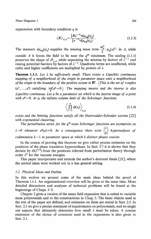
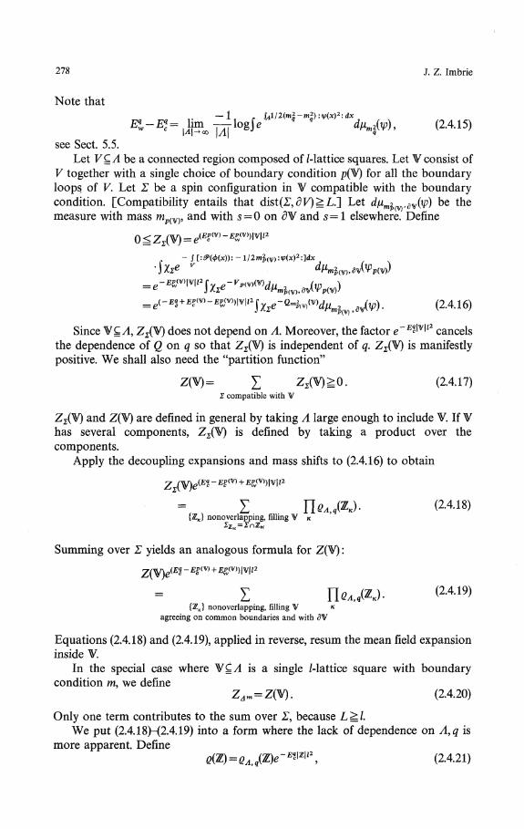
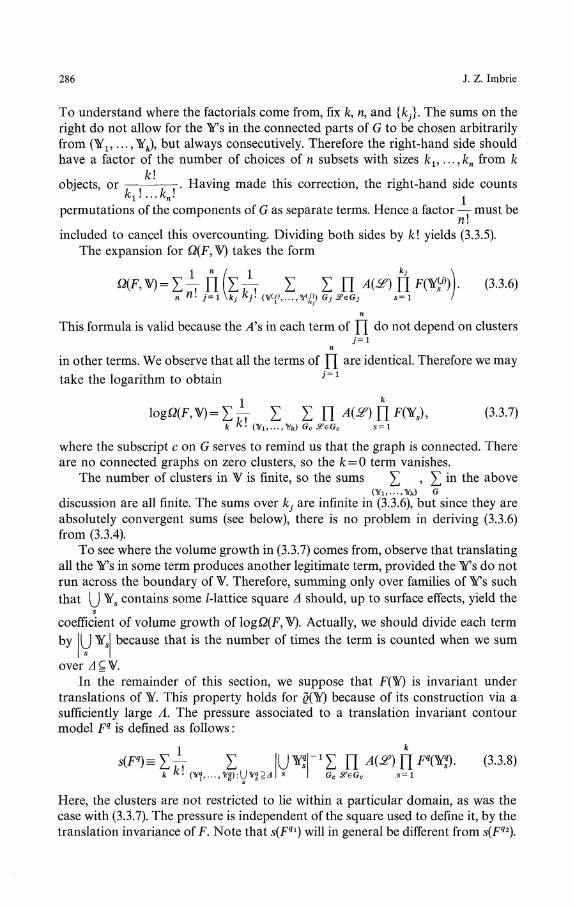
In order to define the subsets of &(Σ\ we construct inductively a sequence ofsubsets of R2:R2=D12D22...2I)II(Σ)+1=0. p(b), the phase of a bond in 8t(Σ)9 isdefined to be the common value of nearby spins. Let D2 be the region bounded bybonds be&(Σ) with p(b)ή=p(bQ)9 where bQ is any bond far outside of A. [Bonds withp(b) = p(b0) may be contained in D2.] Then define Λ£Σ) = &(Σ)n{b : bζD1\D2}. Ingeneral, Dk will consist of a number of connected, simply connected componentsD"k. With b0ζdDl define Dj;+1 to be the region bounded by bonds bgD"k

274 J. Z. Imbrίe
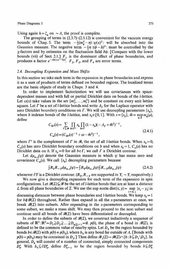
Fig. 2.4.1. The decomposition of 38(Σ) into subsets (̂Γ), @2(Σ)> separated from each other by the
phase boundary Σ
with p(&)Φp(60) and be£(Σ). Then put 0k + 1= (JD£ + ι and #*(£)α
n{&:ί?£D fe\D fc+1}. The construction terminates when the bonds of (St(Σ)are exhausted, and we have a(Σ) = Λ£Σ)\j ... v@n(Σ)(Σ). See Fig. 2.4.1.
We associate to each k a space-dependent mass ωk(x). Define p(Dl)=p(b0)where b0edDl if k^2 and b0 is far outside of A if fc = 1. Then put co^xj^m^^. Weobtain ωfc+ 1 from ωfc by modifying it on each
(using again the sup norm) :
Associated to each ωfc we have a mass-shifted interaction
βωk(Σ, Λ, q) = Q(Σ, Λ,q)+\ \(m\ - ωk(x)) :A
Notice that Qωι = Q.The decoupling expansion uses the identity
: dx . (2.4.3)
for each be&k(Σ) for some fc. For k = l we obtain
ι finite
Σ JdsΓl Σ ί ΠIJ.Γi finite
(2.4.4)
(2-4-5)
Phase Diagrams. I 275
We have used the following notations :
beΓ
et of partitions of Γ,c c
See [7, 17] for details.Before proceeding to the next block of bonds, we shift mass from Q to dμ :
e'Q^μω^SΓι(ψ) = e-^dμ^SΓι(ψ)Zωιω2(sΓι) , (2.4.6)
.̂̂ (sr,)"!*' 1/2(β>lW~<8!l(3e))!*(3t)a!<l"dμ).1..rι(ψ) (2A7)
Absorbing the mass term into dμ changes the covariance to Cω2(sΓl), given in(2.4.1). We shall never apply s-derivatives to Zωι(θ2 factors. As a result of the massshift, contractions to Qω2 from the next block of s-derivatives will bring downpowers of λ.
Proceed through the blocks of bonds &2(Σ)9 Λ3(Σ), ...,&n(Σ}(Σ) shifting mass-squared from ωk to ωk+1 after deriving bonds in $k(Σ). We allow s-derivatives toact on covariances arising from earlier blocks. The result is
Γ finiteΠ=l
Π Zωfcωt+1(sΓk). (2A8)
We have used the following notations :
Γk = Γn
k(α) is the first integer k such that
sb if beΓk
0 if be((l0UΣ)\\Γk
1 otherwise,
sΓ = sΓn,
276 J. Z. Imbrie
We now write (2.4.8) in factorized form. Define Q(Z) as in (2.3.8H2.3.12) butrestricting all integrals to ZnΛ or Zn~A Define βωfc(Z) similarly from (2.4.3).Let {Zκ} be the closures of the connected components of IR2\{s = 0 bonds}. (The5 = 0 bonds are those in &(Σ)\Γ.) Then
We let ΣnZ denote the restriction of the spin configuration Σ to Z, and define
Xmz= ΠΔ\gZc\
so that
Using the fact that Cω(α)(sr) vanishes between Zκ and Zκ,, and the fact that Cω(α)(5Γ)restricted to Zκ depends only on sb with b£ZK, we can apply (2.4.2) to obtain
fΛΓ Σ ί Π f^-β— Ππe^(Γ) j=l αeπ
Tre^ίΓnZK) y = l |
Π \k%CnμrYΔJR^^e-*^dμ^ψ). (2.4.9)
We have assumed that K is a product.The Gaussian integrals Zωkωk+ί(sΓk) also factor, although not as fully as above.
We associate the factors to Zκ's as follows :
), (2-4.10)K
whereωk+ι(χ)> ^ in a connected component of
suppt(ωfc+1 — ω.) whose boundary lies in Zκ
f \ Λ (2A11)
ωk(x) , otherwise .
Notice that suρpt(ωfc — ωj+1) is always separated from suppt(ωfc — ωj'+1)by bonds with sΓk = 0. Hence (2.4.10) is valid. In addition, ZωkωK+ί(sΓl) dependsonly on sΓkn2κ.
Using (2.2.4), (2.3.7), (2.4.8), and (2.4.9), the full mean field expansion becomes
Σ Σ ΠΣ Γg@(Σ),Γ finite K
^> ΠJ
(2.4.12)fc=l
Phase Diagrams. I 277
Note that the construction insures that all spins within L of a connectedDirichlet contour have the same value. If the common value is m, we call thecontour an m-contour. By the locality of the construction of g(x) and ωπ(x),Qωn(Zκ) does not depend on Σr\Zκ, for κ'Φκ;. (It still depends on Λ and theboundary condition q.)
Before making further transformations on (2.4.12), we introduce the notion of acluster. A cluster is a triple (Z,Σ"nZ,ΓnZ) satisfying certain conditions.
(i) Z is a connected union of a finite number of /-lattice squares.(ii) Σ = Σr\Z is a spin configuration in Z.
(iii) Γ = ΓnZ is a set of derivative bonds in Z.(iv) dist(δZuΓ, Σ) ̂ L. Here Σ denotes the phase boundaries corresponding to
the spin configuration Σ.(v) 5ZnΓ = 0.
(vi) Let Γc denote the set of all bonds bφΓ such that dist(b,£)^L. Z\ΓC isconnected.
We use the symbols X, Y, TL to denote clusters. We shall often speak of clustersas if they were simply subsets of R2. Set theoretic operations u, n, \, etc. should beinterpreted accordingly. Let |2£| denote the number of /-lattice squares in TL. Theboundary of a cluster TL consists of a number of loops with boundary conditionsdetermined by Γz, the spin configuration of TL. One loop surrounds all the othersand is called the external loop of TL. Its boundary condition is called the externalboundary condition of TL. If the external boundary condition of Z is m, then TL iscalled an m-cluster.
We define ρA q(Έκ)to be the κ-term of the product over K in (2.4.12). The massshifts, etc. were designed so that ρΛtq(%κ) is determined uniquely by Zκ, Λ, q, andRZκ. (It does not depend on Γn~Zκ or Γn~Zκ.)
We may write (2.4.12) in terms of clusters. Most of the compatibility conditionsamong Σ, Γ, and {Zκ} are handled by (iHvi) above.
J Rs-r dμ.JvJ- Σ Π^,4(ZK) (2-4.13){Έκ} nonoverlapping, filling IR2 K
agreeing on common boundaries, Σ^ = q in %K\Λonly finitely many %K have \ΈK\ > 1
Adjacent clusters must have their Σ's match along common boundaries. Note thatif TL is a single square in ~Λ with no ^-factors, then g(Z) = 0 and ρA q(Z) = l.
At several places in Chaps. 3 and 4, we shall need to resum the expansion(2.4.13) within a region of R2. The sum in (2.4.13) is not a true statistical sumbecause not all the terms are positive. Resummation restores the positivity that isneeded for certain arguments. Resummation also produces the finite volumepartition functions which will be the fundamental objects of study in Chap. 3. Wewill need to make some adjustments in classical energies to allow for the effects ofmass shifts. Define Wick ground state energies
(Recall that mΆ is the Wick-ordering mass, and qe{l9...,r} is fixed throughout.)
278 J. Z. Imbrie
Note that
dμm^' (2A15)see Sect. 5.5.
Let V £ yl be a connected region composed of /-lattice squares. Let ¥ consist ofV together with a single choice of boundary condition p(¥) for all the boundaryloops of V. Let Z1 be a spin configuration in V compatible with the boundarycondition. [Compatibility entails that dist(Z,3F)^L.] Let dμ^ dv(ψ) be themeasure with mass mp(v), and with s = 0 on δ¥ and s= 1 elsewhere. Define
^ (2.4.16)
Since ¥£yl, ZΣ(V) does not depend on Λ. Moreover, the factor e~Eq<^\12 cancelsthe dependence of Q on q so that ZΣ(V) is independent of q. ZΣ(W) is manifestlypositive. We shall also need the "partition function"
Z(¥)= £ Z^¥)^0. (2.4.17)Σ compatible with V
ZΣ(W) and Z(¥) are defined in general by taking Λ large enough to include ¥. If ¥has several components, ZΣ(W) is defined by taking a product over thecomponents.
Apply the decoupling expansions and mass shifts to (2.4.16) to obtain
Σ{TLK} nonoverlapping, filling ¥
Summing over Σ yields an analogous formula for Z(¥):
Σ UQA.M- (2A19)
{ΊLK} nonoverlapping, filling ¥ Kagreeing on common boundaries and with 5¥
Equations (2.4.18) and (2.4.19), applied in reverse, resum the mean field expansioninside ¥.
In the special case where WQΛ is a single /-lattice square with boundarycondition m, we define
(2.4.20)
Only one term contributes to the sum over Σ, because L ̂ /,We put (2.4.18)-(2.4.19) into a form where the lack of dependence on Λ,q is
more apparent. Defineq^l\ (2.4.21)
Phase Diagrams. I 279
where A has been taken large enough so that TLζ.Λ and dist(cM,3Z)^:L. As withZΣ(V), the e~E*W2 factor cancels the dependence on q, making ρ(K) independent ofA and q. Equations (2.4.18) and (2.4.19) may be rewritten as
{Zκ} nonoverlapping, filling VΣz" = ίnZκ (2.4.22)
£ ΠβW-{Έκ} nonoverlapping, filling V K
agreeing on common boundaries and with 3V
2.5. Vacuum Energy Estimates and Bounds on Terms of the Expansion
In this section we state the main technical estimates used in Chaps. 3 and 4. Theproofs will be deferred to Chap. 5.
The most important estimate is the vacuum energy bound. It providesestimates uniform in λ, despite the fact that the classical energies E™ are 0(λ~2)relative to one another.
Let (n(Δ\)} be a set of nonnegative integers, one for each Δ\ξ* Yr\Λ. Define
and put
X&r= Π xSf'W1))- (2-5.2)
Let |Σ'| be the number of Δ\ with n(Δ\)Let \Ύ\m be the volume (in units of /2) of the portion of Y with Σ = m, and let
151= ΣlyL Recall that m= supmq(μ).m <l*V
Proposition 2.5.1. There exists £>0 such that for all C>2, ?/e(0,ζ/4] there existsτ2Of,C)>0, φ,C)>0, and λ0(η,C)>0 such that for all λe(0,Λ0], all
ηλ,μ>ζv-'iζr} ζηC-admissible and all pe 1,1 +
30m2
e \\LP(dμωn>Sr(ψ))
y Γiίvq — £m\|y|
c ' -
The Lp estimate is needed so that we may be able to split a general integral into aGaussian part times an integral as above via Holder's inequality.
The next proposition provides a lower bound needed to support the interact-ing measure and prevent normalization factors from vanishing.
Proposition 2.5.2. With £, C, η, α, A, and 0>λfμ as in Proposition 2.5. 1 except that λ0
depends also on /,(2.5.4)
280 J. Z. Imbrie
We next state bounds on the terms of the mean field expansion. First considerthe case where there are no field monomials, that is, R = 1. Clusters with no fieldmonomials will be denoted by the letter Y. For the others we use the letter X Letp(TL) denote the external boundary condition of Z. If mφp(Z), define DntwZ to bethe region bounded by boundary loops of 7L that are in the mth phase. Everycomponent of IntmZ is given boundary condition m.
Proposition 2.5.3. Suppose λ<ζl<ζl. There exist τ1(η,C)>0, τ2(η,C)>0 such that
| Ym| Σ (E? ~ E® - EξM + £^V))/2|ihtm Y|-e e»«*p(Y) . (2.5.5)
Take R to be of the form
R=ίl ψJ(xfl , (2-5.6)
'and let degβ = Σ ^i Let || \\LP> denote the norm for Lp \Y[ Ai L where At is thei=l \ / = l /
/-lattice square containing xt. (The J/s need not be distinct.) Assume that ^.gXforall i. Define N(A)= £ fef.
i:Δi = A
Proposition 2.5.4. Given p'e [1, oo), let λ <ζ 1 <^ /. There exist positive constants τί9 τ2,K depending on p'9 η, C such that for degR^ 1, |X| ̂ 1,
^ (2.5.7)
// Σx=m, fhen the factor A~degΛ may be omitted.
Differences such as E™ — E™ appear because of the mass shift normalizationfactors included in the definition of QΛfq(%). These factors will extend into ΠntmZ.
The next two propositions give some smoothness in μ to elements of theconstruction of Chap. 3. They are needed in Sect. 3.7, where the phase diagram isconstructed.
Proposition 2.5.5. Suppose λ<ζl<ζl. There exist τ1(η,C)>Q, τ2(η,C)>0 such that
Y|
Phase Diagrams. I 281
Proposition 2.5.6. With ζ, C, η, λ9 and \μ as in Proposition 2.5.1, there exists K(η, C)such that
Λ i *v&\*-'λΛ v / w / = •«•»-"' * ι v ι \Z.J.y)
Without Proposition 2.5.6, only limited information on the phase diagram maybe obtained - see [21].
In the next two chapters we shall use extensively the following normalized form
(2 5' (
Using Propositions 2.5.2-2.5.4, we see that the energy factors cancel, yielding thebounds
Δ
-de8*, Γχφm
1, Σ^ =
In case TL is well inside Λ, (2.4.21) implies
= ρ(Z), (2.5.12)
where we have made the Λ9 ^-independence clear by dropping the subscripts on ρ.
3. The Search for Stable Phases: Ratios of Partition Functions
3.1. The Physics: Surface Energies and Collapsing Expansions
Chapter 3 constitutes the core of this paper. The main result to be proved is thefollowing bound on ratios of partition functions:
_ZW_<e*ι"Ί"l (3 I DZ(Wqo) ' lAi.i;
Here ¥ and ¥α° occupy the same simply connected region in 1R2 but ¥^° hasboundary condition qQ. The fact that (3.1.1) holds for arbitrary ¥ for some
: {1,..., r} will be of the utmost importance in all subsequent developments. It is
282 J. Z. Imbrie
the definitive sign that q0 is a stable phase at a given point in parameter space. Onecould not hope to give a convergent expansion for Schwinger functions withoutfirst attending to a bound of this type.
Pirogov and Sinai [23, 24] have developed a technique for obtaining boundslike (3.1.1) in theories lacking the special properties discussed in the introduction(symmetries, correlation inequalities, or large differences in classical energydensities). Their work applies to lattice spin systems where the spins take values ina finite set. We adapt many of the ideas in [23, 24] for the problem at hand. Weencounter additional problems from the unboundedness of φ and from the contin-uum limit. In Chap. 4 we deal with a third additional complication : In contrast to[23,24], the passage from (3.1.1) to a construction of the stable states is nontrivial.
The difficulty in proving (3.1.1) lies first of all in the fact that both numeratorand denominator have exponential dependence on the volume of ¥. Yet the boundstates that Z(Wq°) dominates up to a small surface term. Second, there is no a prioriway of knowing which phases q0 should work in (3.1.1).
Heuristically speaking, the stable phases should be the ones of least energy.There is, however, no simple measure of the energy of the unstable phases. Forexample,
(3 L2)
is presumably the same for all m, because the theory should tunnel into a stableminimum if unstable boundary conditions are imposed.
A way of constructing a measure of the energy of unstable phases is given byPirogov and Sinai in [24]. A theory is first expressed in terms of contoursseparating uniform distributions of spins. Unstable boundary conditions m shouldbe characterized by the fact that fluctuations out of the mth state should have a
probability growing like — ̂ — ea^ Volume of contour|, for some αm>0. The constantNorm.
am is a measure of the energy of the mth state.In order to achieve a situation where the partition function is given by such an
ensemble of contours, one must proceed through successive approximations to cΓ.In our ^(φ)2 model,
am= -\ogZAm- infί-logZ^) (3.1.3)
is an excellent first approximation, as it contains the Wick ground state energy andalso some fluctuations about the mth minimum.
When one attempts to describe the theory using this approximation to therelative energies, one finds two types of errors. The approximate partitionfunctions we use have an expansion
Iogί2(¥) = s|¥| + zl(¥), (3.1.4)
where the pressure s is independent of ¥ and where |zl(¥)|^/l1/2|d¥|. A differenceof pressures corrects the first approximation to {αm}. Surface energies A(W) must beincorporated into the description of the theory by including them with the"energy" of contours bounding ¥.
Phase Diagrams. I 283
After making the corrections, the new approximate partition function isexpanded as in (3.1.4) and the procedure is repeated. As one proceeds through theiteration, higher and higher order surface effects are taken into account. When theiteration converges, one has a description of the true partition function Z(V) interms of an ensemble of contours with factors e*mlVolume of contourl. The phases q0 forwhich aqo = 0 can then be shown to dominate the others as in (3.1.1). If severalphases have aq° = Q at some point in parameter space, then they will all coexist atthat point.
Collapsing expansions are the principal tools for carrying out the proceduredescribed above. They arise from the following construction.
Compatibility of clusters on shared boundaries is a very difficult condition towork with. Therefore, one resums the mean field expansion inside the outermostclusters (the ones not surrounded by other clusters). The result is a partitionfunction Z(V) for the regions surrounded by clusters. If the outer clusters are
Z(V)multiplied by — Z(Vq) and if Z(Vg) is expanded in the numerator, then one
returns to the original boundary condition q and there is no compatibilitycondition for the outer clusters.
To be completely relieved of compatibility conditions, one must apply theabove procedure to the clusters that make up the expansion for Z(Vβ) andcontinue to smaller and smaller clusters. In the end, one has an expansion purelyin terms of ^-clusters with no compatibility conditions. Each cluster is multipliedby a ratio of partition functions. This form of the expansion makes it clear why(3.1.1) is so important.
One can reverse the above procedure to recover the original expansion. Whenthis is done, we say the expansion has collapsed.
Collapsing expansions were first used in quantum field theory in [20]. Theywere used to make the step from Z/Z bounds to a cluster expansion, rather than toprove Z/Z bounds.
The biggest problem we encounter lies in bounding partition functions thatinvolve the factors e«
mlVolumel. Only the crudest estimates are available for suchobjects. (A more familiar situation is where contours have probability e-
tlLensthl> in
which case expansion techniques give very precise bounds.) The crude boundsdepend on every term in the partition function sum being positive. Unfortunately,ρ(Y) is not in general positive.
We discuss this problem in greater detail in Sect. 3.4. The resolution of theproblem entails that each iteration step consist of an inductive constructiondesigned so that the expansion may be collapsed at any point. Certain bounds areproven in the collapsed form of the expansion, while others are accomplished inthe uncollapsed form. The constants αm acquire a dependence on the diameter ofclusters.
A second major problem arises in proving smoothness of the construction inthe parameters of £P. Smoothness is needed to solve for the parameters that yieldan arbitrary set of αm's, as was done in [24]. The difficult bound is Proposition2.5.6. One must control the bounded-spin approximation for φ and obtain lowerbounds on ZΣ(V). These problems will be covered in Chap. 5.
284 J. Z. Imbrie
3.2. Contour Models
In this section we introduce certain statistical ensembles which will be usedthroughout this chapter. Recall the definition of clusters given in Sect. 2.4. In mostof this chapter we restrict attention to clusters with more than one /-lattice square.
Definition. Let F be a real-valued function of clusters. F will be called a contourfunctional if
\\F\\ = supeτ ι /l¥l+ τ 2 λ"2l^l|F(¥)|<oo. (3.2.1)
The restriction of F to q-clusters will be denoted Fq and called a q-contour model.\\Fq\\ is defined by restricting the supremum in (3.2.1) to q-clusters. Note that F(Y)need not be positive.
Let Y be a finite, connected, simply connected union of l-lattice squares togetherwith a choice of boundary condition. Such a Y will be called a simple domain. Adomain is a finite union of simple domains. The components of a domain may havedifferent boundary conditions. |Y| will denote the number of l-lattice squares in ¥ and|δ¥| will denote the number of l-lattice bonds in the boundary of ¥
For any contour functional F, we define a partition function as follows.Suppose ¥ is a simple domain with boundary condition q. Then
(3.2.2)s
Y| g V, nonoverlapping
The sum over {Yf} is over collections of nonoverlapping g-clusters in Y, and|Yf|>l. If {Yf} = 0, the product is set equal to 1. Note that every cluster in thecollection has the same external boundary condition as ¥ and that neighboringclusters may disagree on boundary conditions. This is different from the expansionof Sect. 2.4, where neighboring clusters agree, and where clusters with any externalboundary condition may appear.
To define Ω(F,¥) for general domains, let {¥.} be the simple domains thatmake up ¥. Then
(3 2 3)
An example of a contour functional is ρ, with no field monomials presentCR = 1). [See (2.5.10) and (2.5.12).] From (2.5.11) we see that ρ(Y) has the requisitedecay. In fact, there is room to spare in the exponential bound on |ρ(Y)| so that
FL(Y)Ξρ(Y)e^> (3.2.4)
is also a contour functional if L(¥)^τ1ί|Y|.Much of this chapter is devoted to finding an L(Y) such that the true partition
function is given by) = Ω(FL,W). (3.2.5)
This will only be possible if ¥ has thermodynamically stable boundary conditions.(For the other boundary conditions, we will need the generalized contour modelsintroduced in Sect. 3.4.) L(Y) will be a sum of several terms, one of which is
) for some F and for ¥ a domain surrounded by Y. In order to preserve
Phase Diagrams. I 285
the bound LίY^τJIYI we will have to cancel the volume growth of logΩ andleave just a surface term. In the next section we will show how to separate thesurface effect from the volume effect and obtain bounds on each.
3.3. Expansions for the Pressure and Surface Energy
We make use of some algebraic properties of partition function sums in order towrite Ω(F, V) as an exponential of some quantity. Then taking the logarithm andseparating surface effects from volume effects will be easy. The main barrier totaking the logarithm of the expansion (3.2.2) is the constraint that no two clusterscan overlap. Following [1], we implement the constraint using functions ofclusters £7(Y15 Y2). The technique can be traced back to similar ideas in statisticalmechanics [26] and in quantum field theory [8]. The l/'s defined here are specialcases of ones in Chap. 4.
Define
,33 ̂1 otherwise. l ' ' }
Assume ¥ is a simple domain with boundary condition q. Then the expansion forΩ(F,V) (3.2.2) becomes
£ Y[ U(Yq
Si,Yq
S2)YlFq(Ύ«). (3.3.2)k *>' (¥?,...,¥«) sι<s2 s
We have changed from summing over sets of Yfs to summing over orderedfamilies of Yfs, hence the 1/kl. The terms in this sum involving only nonover-lapping Yfs are unchanged, while the others vanish. In the remainder of thissection it will be assumed that all clusters have external boundary condition q andthe superscript q will be omitted.
Define some more operations A = U — l, and expand the product of l/'s usingthe formula
(3.3.3)
Here ίf is a set of unordered pairs of clusters (called lines <£). G is a subset of £fand can be visualized as a graph connecting clusters with the lines &. Equation(3.3.2) becomes
Ω(F> v) = Σ A Σ Σ Π ̂ ) Π TO (3.3.4)k K. (γ l 5...,¥k) G &<=G s
A graph G is called connected if the lines in G form a connected graph joining allthe clusters in G. Every graph breaks into its connected components (which mayconsist of single clusters with no lines). Let G15 ...,Gn be the connected com-ponents of G. We sum separately over the Ys's and G/s in each component, usingthe identity
ΣTΓ Σ Σ^Σ^ήίΣίTT Σ Σ) (3 3 5)k K (¥ι,...,¥k) G n n- j=l\kj ^j (¥φ,... ,¥(£) Gjl
286 J. Z. Imbrie
To understand where the factorials come from, fix k, n, and {ky}. The sums on theright do not allow for the Ifs in the connected parts of G to be chosen arbitrarilyfrom (Ύ1? ...,Yfc), but always consecutively. Therefore the right-hand side shouldhave a factor of the number of choices of n subsets with sizes k1? . . . , fc n from k
klobjects, or ——'—j—r Having made this correction, the right-hand side counts
k t . ...kn. ^permutations of the components of G as separate terms. Hence a factor — must be
included to cancel this overcounting. Dividing both sides by k! yields (3.3.5).The expansion for Ω(F, ¥) takes the form
Ω(^=Σ-Jτ Π (Σ^ Σ Σ Π AW ft W)). (3.3.6)n n- j=ί\kj K j l (γO),...,γU)) Gj &eGj s=l I
n
This formula is valid because the A's in each term of ]~[ do not depend on clusters7=1
n
in other terms. We observe that all the terms of Y\ are identical. Therefore we may
take the logarithm to obtain -7"1
logΩ(F,V) = Σ^Γ Σ Σ Π Λ(^) Π W), (3.3.7)k Kl (γ l f...,γk) Gc JS?εGc s=l
where the subscript c on G serves to remind us that the graph is connected. Thereare no connected graphs on zero clusters, so the k = 0 term vanishes.
The number of clusters in ¥ is finite, so the sums £ , ]Γ in the above(Yι,.. ,Yk) G
discussion are all finite. The sums over kj are infinite in (3.3.6), but since they areabsolutely convergent sums (see below), there is no problem in deriving (3.3.6)from (3.3.4).
To see where the volume growth in (3.3.7) comes from, observe that translatingall the Ifs in some term produces another legitimate term, provided the Vs do notrun across the boundary of ¥. Therefore, summing only over families of Y's suchthat \J Ys contains some /-lattice square A should, up to surface effects, yield the
s
coefficient of volume growth of logί2(F,¥). Actually, we should divide each term
by because that is the number of times the term is counted when we sums
over zJg¥.In the remainder of this section, we suppose that F(Y) is invariant under
translations of Y. This property holds for ρ(¥) because of its construction via asufficiently large A. The pressure associated to a translation invariant contourmodel Fq is defined as follows:
1 k
— V V l l l ¥ ί ! ~ 1 V Γ Γ A(Ψ\Y\ Fq(Ύq} Π 3 8Ϊ== / / \\ I **• n / I I •ίlloZ' ) I I L \ J l o , / . \J.J.OIZ-ί/. i Z-< W s z_ί 1 1 v / i l v s/ ^ ^
Here, the clusters are not restricted to lie within a particular domain, as was thecase with (3.3.7). The pressure is independent of the square used to define it, by thetranslation invariance of F. Note that s(Fqι) will in general be different from s(Fq2).
Phase Diagrams. I 287
Subtracting sOF4)!"^ from logΩ(F,¥) should leave a remainder growing asDefine
Δ(F, V)=logΩ(F, V) -
Σ(Yι, . . . ,Yk) , ,
Vn (J Ys Φ 0 Φ ~ Vn (J YS
Σ Π Π F W (3 3-9)
The second line follows from (3.3.7) and (3.3.8). All the terms of (3.3.7) arecancelled, leaving graphs containing squares of both ¥ and ~¥. These do notappear in logΩ(F,V)9 but appear exactly ¥n (J ¥s times in s(Fq)\W\.
s
If V has several components ¥ , each with the same boundary condition, define
We now estimate the pressure and surface energy, using a lemma proven inSect. 4.4.
Lemma 3.3.1. Suppose λ<ζ 1 <ζl. If Fq is any q-contour model with \\Fq\\ ^ 1, then
Σ Σ Πk
Π ^k\\\Fq\\e~Til(k+N)/4. (3.3.11)
There are two sources of convergence. The first is that ,4(Y1? Y2) = 0 unless Ύ1
overlaps ¥2. The second is the exponential decay of F(¥) with |¥| and with \ΣΎ\[see Eq. (3.2.1)].
Proposition 3.3.2. Supposemodel with ||Fβ||^l. Then
l. Let Fq be a translation invariant q-contour
\s(F*)\£\\F*\\, (3.3.12)
where s(Fq) is defined in (3.3.8). Moreover, if ¥ is a domain with only q-boundaryconditions, then
with
\A(F,W)\^\\Fq\\ \dW\ (3.3.14)
and Λ(F,W) given by (3.3.10) and (3.3.9). Finally, if F\ and Fq
2 are two q-contourmodels as above, then
\s(Fq)-s(Fq
2)\ ^ \\F\ -F\\\ (3.3.15)
and
\A(Fl,W)-A(Fq
2,V)\^ \\F\-Fl\\\dV\. (3.3.16)
Proof. By summing over fc^l and NΞ>2 in (3.3.8) and applying the lemma, weobtain (3.3.12). Every graph in (3.3.9) must contain a square at the boundary of ¥.
288 J. Z. Imbrie
Applying Lemma 3.3.1 to each such square, and usingY.
5g 1, we obtain
the bound |J(F,¥)|^ \\Fq\\ \dW\. Equation (3.3.14) follows by summing over thecomponents of ¥. To prove (3.3.15), interpolate between F± and F2 in the formulafor s(Fq). Let F?(¥) = ίF|(¥) + (l-ί)F«(¥). Then
\s(Fl)-s(Fl)\ =
?2J s
^ \\FI-F\ 'k\
1ΣU
Σ Π x& Π
Σs=l s = l
S Φ S
k
s=l
(3.3.17)
where F«(Y«) = e"τιI|γ2 |"τ2λ"2|ι;v-1. The sum over s is controlled by -i , and we
have used ||Ff|| ^1. Applying Lemma 3.3.1 as before, we obtain (3.3.15).For (3.3.16), interpolate as above. The sum over squares A lining δ¥ yields the
factor |δ¥|, as in (3.3.14). The factor k from the sum over s is controlled by e~τίlk/s,
taken out of (3.3.11). Π
3.4. Contour Models with Parameters : An Inductive Construction
In this section we introduce ensembles whose purpose is to describe the unstablephases as well as the stable ones. The basic idea is as in [24]. Contour functionalsare multiplied by factors that grow exponentially with the volume of interiors ofclusters. The coefficient of volume growth can be thought of as the loss in energydensity (gain in probability) achieved by fluctuating into a stable phase. The resultis not a contour functional, but the new partition function can be crudelydominated by the old one times an exponential factor. When we have managed toexpress the partition function of our 0*(φ)2 model as a partition function for acontour model with parameter, the crude bound will yield the ratio of partitionfunction estimate that this chapter is devoted to.
Carrying out the above plan in the context of quantum field theory producessome problems. The most serious is the fact that ρ(¥) is not in general positive.Therefore, multiplying terms of associated partition function sums by factorsgreater than 1 does not necessarily increase the sums. There is, however, a form inwhich the mean field expansion has positive terms. This is after the expansion inspin configurations, but before the introduction of decoupling lines. Our strategywill be to multiply terms of the expansion by volume-divergent factors when it isthe undecoupled form, and then use the decoupled form to make estimates thatdepend on decoupling. In order to work things so that one can go back and forthbetween the two forms at any time, we are forced to use a rather complicatedprocedure. We must exploit at each stage the collapsing expansions that resultwhen terms are multiplied by ratios of partition functions. (In [24] a collapsingexpansion was obtained only after the iterations had converged.)

Phase Diagrams. I 289
We will work with contour functionals FL, where
(3.4.1)
and where certain growth conditions are imposed on L.
Definition. Let (5(Y) denote the largest dimension of Y, measuring distances in unitsof I along the directions of the l-lattice. We call δ(Ύ) the diameter of Y. L, a real-valued translation invariant function of clusters, is called a vacuum functional if
:α) (3A2)
and^(Y)^^/|Y|. (3.4.3)
In d dimensions, we would use δ(Ίf)d+ί in place of (5(Y)3. We could also use thenorm of [24] which allows |L(Y)| to grow exponentially with |Y|. Our strongergrowth condition is possible because in the iteration of Sect. 3.6, errors accumulatemore slowly with δ(Y) than they do in [24].
The splitting of FL into ρ and eL avoids the problem of taking the logarithm ofρ. Notice that eL(¥)canbe very small, but it cannot be very large, by (3.4.3). From(2.5.11) we have that FL is a contour functional if L is a vacuum functional.
(3A4)
Given a contour functional FL, define for each q
aq(FL) = - s(Fi) - logZJβ + const, (3.4.5)
where the constant is adjusted so that
mfaq(FL) = Q. (3.4.6)
From (3.4.4), Proposition 3.3.2, and Proposition 2.5.2, we see that up to 0(λ112)corrections, aq(FL)/l2 is the Wick ground state energy of the qih well of & relative tothe smallest such energy. Thus aq(FL) may be as large as O(λ~2l2).
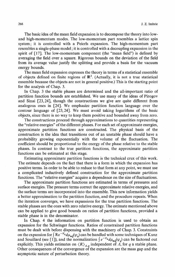
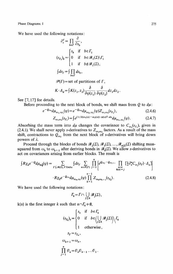
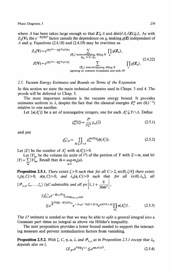
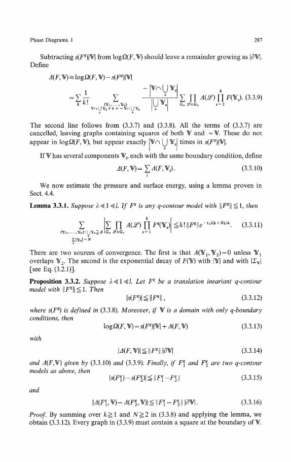
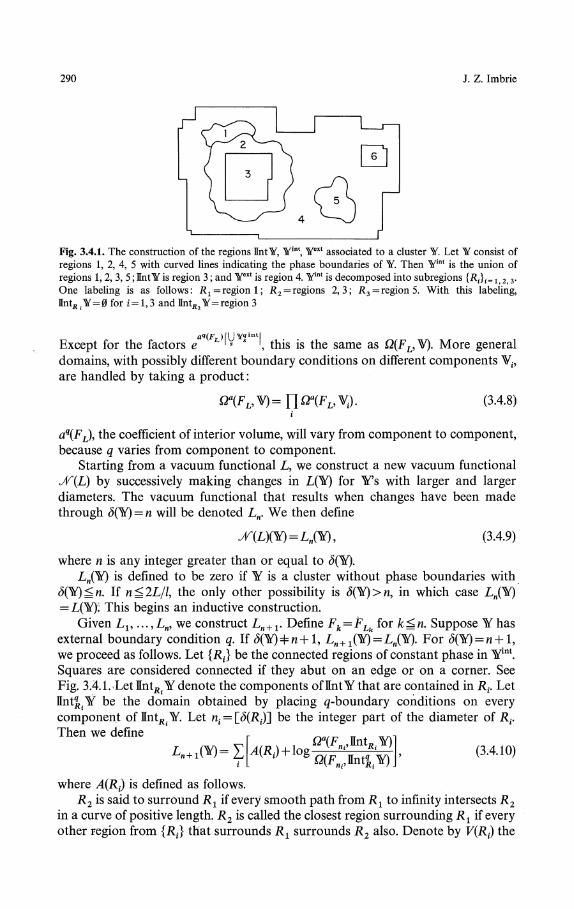
Definition. The interior domain of Y, denotedΉntΎ, is defined as follows. Suppose Yhas external boundary condition q. Consider the closure of the union of all theq-squares of Y (the ones with p(Δ 1 ) = q). Of its connected components, let Yext be theone bordering on the outer boundary of Y. Call a boundary loop of Y inner if it is notcontained in Yext. Int Y is defined as the region bounded by the inner loops of Y, witheach component given the boundary condition associated to the loop bounding thatcomponent. |Πnt Y| will denote the number of l-lattice squares in Int Y.
Define Yint = (YuIntY)\Yext. Γ¥int, the spin configuration associated withYint, is defined by extending Z"YnYint to Int Y so that the phase that exists on theboundary of a component o/IntY persists in all of that component. See Fig. 3.4.1.
We define the partition function for a contour model with parameter in amanner closely related to Eq. (3.2.2). If Y is a simple domain with boundarycondition q, then
Σ ΠW)^)|yV?Ί (3-4.7){¥«} s
Y| ς V, nonoverlapping
290 J. Z. Imbrie
Fig. 3.4.1. The construction of the regions Πnt Y, Yίnt, ¥ext associated to a cluster Y. Let Y consist ofregions 1, 2, 4, 5 with curved lines indicating the phase boundaries of Y. Then Yίnt is the union ofregions 1, 2, 3, 5 UntY is region 3 and Yext is region 4. Yint is decomposed into subregions {.Rf}ί= l f 2,3-One labeling is as follows: Rί= region 1; R2 = regions 2,3; R3= region 5. With this labeling,Πntjj. Y= 0 for i = 1,3 and ΠntΛ2 Y= region 3
aq(F -ΊV Y« ln
Except for the factors e L ls s ', this is the same as Ω(FL,V). More generaldomains, with possibly different boundary conditions on different components ¥ί?
are handled by taking a product:
V.). (3.4.8)
α%FL), the coefficient of interior volume, will vary from component to component,because q varies from component to component.
Starting from a vacuum functional L, we construct a new vacuum functional^(L) by successively making changes in L(Y) for Ys with larger and largerdiameters. The vacuum functional that results when changes have been madethrough d(Y) = n will be denoted Ln. We then define
(3.4.9)
where n is any integer greater than or equal to c)(Y).LΠ(Y) is defined to be zero if Y is a cluster without phase boundaries with
δ(Ύ)<.n. If n^2L/l9 the only other possibility is δ(Y)>n, in which case LK(Y)= L(Y); This begins an inductive construction.
Given L1? ...,Ln, we construct Ln+1. Define Fk = FLk for k^n. Suppose Yhasexternal boundary condition q. If <5(Ϋ)Φn+l, LΠ+1(Y) = LΠ(Y). For (5(Y) = rc+l,we proceed as follows. Let {R^ be the connected regions of constant phase in Y1111.Squares are considered connected if they abut on an edge or on a corner. SeeFig. 3.4.1. Let Intβ.Y denote the components ofϋntYthat are contained in Rt. LetΠnt|.Ϋ be the domain obtained by placing ^-boundary conditions on everycomponent of Int^.Y. Let ^ = [(5(1̂ )] be the integer part of the diameter of R{.Then we define
I U"f h llnt_ \Yl I
(3.4.10)
where A(Rt) is defined as follows.#2 is said to surround R1 if every smooth path from R{ to infinity intersects R2
in a curve of positive length. #2 is called the closest region surrounding Rl if everyother region from {R.} that surrounds R1 surrounds R2 also. Denote by HR^) the
Phase Diagrams. I 291
volume (in units of/ 2 ) of the union of Rt with all the regions surrounded by Rt. Letp(Rt) denote the phase of JR£ and let m(Rί) denote the phase of the closest regionsurrounding Rt. If no regions surround Ri9 then m(Ri) = q, the phase of Yext whichsurrounds all the regions.
If Rt is not surrounded by any other R, then
Γ 7 1
(3.4.11)
Otherwise, let Ri2(R.) be the closest region surrounding .R .̂ Then
(3.4.12)
This completes the inductive construction.Notice that the construction of Ln+ x used F19 . . . , Fn9 not just Fn. The reason is
so that when we assemble a set of clusters with their factors eL, the am(Rί\Fn)coefficients associated with various regions will depend only on Σ9 and not on Γ.This will permit us to resum the decoupling expansion, leaving only an expansionin phase boundaries where all terms are positive.
To prove that the construction does not produce LM's that are not vacuumfunctionals, and to obtain useful properties of the Ω's, we state a proposition andcarry it along as an inductive hypothesis.
Proposition 3.4.1. Suppose λ<ζl<ζl. Let L be any vacuum functional, and for any nlet Lί,L2,...,Ln be constructed from L as described above. Then Ll9 ...,Ln arevacuum functionals, and \\\Lk\\\^\\\L\\\ + 0(λ~2l2) for ί^k^n.
Suppose Y is a simple domain with diameter <5(V) and boundary condition q. Arepresentation for Ωq(Fj,W) may be obtained for j^n as follows. For any spinconfiguration in ¥ define regions Rt as in the construction given above. Define ni9
p(Ri), m(Rt)9 and i2(Ri) as above. If Ri2(Ri) does not exist, then set ni2(R.} =j. If <5(¥)then
(3.4.13)Σnv 1 1 Z
compatible with V A c v
The ordinary contour model partition function Ώ(F p ¥) is given by the same formulaexcept that for i such that -Rίa(Λί) does not exist, the corresponding term in Y[ has
am(Rί\FΛi2(RJ replaced by zero. By the nonnegativity of ZΣ, we have l
¥) ̂ Ω(Fp V)ea9(F^ . (3.4. 14)
Proof. To avoid confusion, we suggest setting E™ = E™ and Z J W=1 for a firstreading. We proceed by induction on n. For small n, Ln(¥) = L(¥) or zero, and thebound on \\\Lk\\\ is trivial. There can be no phase boundaries in ¥, so HntY= Yint
= ̂ = 0 for all Y£¥. Therefore, Ωa(F p ¥) = Ω(Fp ¥) = Ω(ρ, ¥). The decouplingZ _ (¥)
expansion for ^q is exactly Ω(ρ,¥), so (3.4.13) follows.1 1 Zj*
292 J. Z. Imbrie
To prove the proposition at stage n, suppose it holds for n<n. We need thefollowing bounds on LW(X), for δ(\) = n:
¥|. (3.4.15)
Suppose Y has external boundary condition q. Visualize the accumulation ofterms in £ A(Rt) as follows: For each i, A(Rt) associates terms ± am(Ri\F)/l2 and
— to every unit square contained in, or surrounded by, Rt. Many of the1 ZΔP(Rί)
1
T2± — logZA terms cancel. If Rl surrounds or contains a unit square and R2 is the1' 1-^-logZ.p^) cancels with —-r r
closest region surrounding R19 then ^-logZJjp(jR2) cancels with - —logZJm(R.).
The only uncancelled terms are -ylogZ^R^) and —^-logZ.q, the latterI ~ r
coming from the region with no R{ surrounding it.
The terms ± am(Rί\F)/l2 in (3.4.12) would cancel if Fn. were the same as Fn.2(R).Keep track of them as follows. For each unit square A1 of Yint, let Riί(Ai) be trieregion containing A1, and let Ri2(Aί),Ri2(Aί), ...,Riω(A1) be the successive regionssurrounding A1 such that each one is the closest region surrounding the last. SinceiΛ(Δ^) is independent of A1 as long as A1 is chosen from a fixed region, we candefine more generally 1Ά{X) = ίJ(Al £X) ίorX a subset of some 1̂ . This agrees withour definition of /2(^i) above. Riί(Ai), •• »^iω_1(ji) contribute differences of tfs andRi(o(Ai) contributes only —aq(Fn. (Δ1))/12 We have derived the following equation:
ύ=- Σ Σ (am(R^\Fnί +ιul))
(3.4.16)
Consider first the terms zl^Y^nY. The difference of α's is small becauseFn. differs from Fn. only on clusters with diameter larger than nt . Thus for
eveVyphasep, " i^j-^y^i^-^ii
^g-tικ»,.+ D^ι/2 φ (3.4.17)
We have used Proposition 3.3.2 and the fact that ρ has extra exponential decay[see (2.5.11)] so that the possible growth from eL and the large factor in the normcan be dominated and a factor e~
τίl(nia+1) remains. Using the definition of am
(3.4.5)-(3.4.6), we obtain
! )\-ζ2λί/2e~τιl(ni«(Δί)}
Therefore,
,-C -̂lα = l
(3.4.19)
Phase Diagrams. I 293
We are using the fact that Fn.χ and Fni<χ+ι differ only on large clusters for large α.Hence the corresponding change in a is small.
The terms -α^ + logZ^-logZ^ are handled by noting that
α* - ap = s(Fp) - s(F9 + logZΔP - logZΔq , (3.4.20)
so that) - s(Fp)
. (3.4.21)
Hence the contribution to L from A1 Q Y is bounded by 0(Λ1/2)|Y].Next consider zl1 £¥, where ¥ is a simple domain of UntΎ. We bound
α = l
as before, but noting that niK(Ai)^o(W), which greatly reduces (3.4.17). Equation(3.4.19) becomes
ω(Al)-ί
Σ (am(RiβtiΔiy)(p \\ \ "i«+ι(Δί)'
τιίW. (3.4.22)α = l
Summing over zl^V and over VgllntY yields a bound 0(/11/2)|¥| for thecontribution of these terms, since the number of components of IntY is less than|¥|.
Up till now we have been bounding the effects due to making the α-factorsdepend only on spin configurations. We next attend to the contribution from theratio of partition functions, which is physically the interesting term. Consider eachsimple domain ¥ of Unt Y separately. Note that ΰ = wίl(v) < n because δ(Ril(v)) ^ <5(¥)-2L. Thus we can apply an induction hypothesis from Proposition 3.4.1 :
(F,, v) ^ (3.4.23)
Here p(¥) is the phase of ¥, and we have used Proposition 3.3.2. In addition,
(3.4.24)
where Wq is ¥ with boundary condition changed to q. We can now bound theremaining contributions to Ln from ¥ as follows :
- s(Fϊ) - a«(Fnί^) + log ZΔPW - logZ,,)
= Δ(F-n, V) - A(F-n,
|e- τ'ίί(V)
(3.4.25)
294 J. Z. Imbrie
Using the definition of the α's, we see that all of the volume factors would havecancelled exactly, except for the difference between aq(F^ and fl%F,,ie(V)). Thisdifference is bounded as in (3.4.18). What remains is a surface effect. This near-cancellation of volume effects is simply the result of a judicious choice of volumeterms in L. Summing over YglintY, and using the other results above, we obtainthe bound Ln(Ύ)^0(λ1/2)\Ύ\.
We proceed to the lower bound on LM(Y). Except for (3.4.25) and (3.4.21), all ofthe above bounds are bounds on absolute values and can be used for the lowerbound. From (3.4.14), we have
Ωa(FfrW) ^Σ = qW
l)\\\. (3.4.26)
In the last step we have used the decoupling expansion to show that
Σ{Yf } : Iγ«= 0 , nonoverlapping s
(3.4.27)
where F0(Y) = ρ(Y) if ' ΣΎ = 0 and F(Y) = 0 otherwise. Since ||F0||Proposition 3.3.2 yields (3.4.26).
The other terms -αβ(FBiβ(V))+logZdP(V)- logZ^ occurring in (3.4.25) and(3.4.21) are bounded below by 0(λ~2l2). Altogether we have
^-0(/T2/2)(5(Y)2. (3.4.28)
Thus |||Ln(¥)|||^0(A-2/2) + |||L|||. We include |||L||| in this estimate because of
contributions to Ln from Ys with <5(Y) > n. The need for the 3 factor in thedefinition of |||L||| will not appear until later in this chapter. ^ '
We now prove (3.4.13) and the analogous statement for Ω(FJ9W). The proof isthe core of our construction. Four basic steps are involved. The expansion forΩα(Fj, ¥) is collapsed, and the induction hypothesis is applied for EntY with Yg V.Then after a complicated matching and cancellation of volume factors, thedecoupling expansion is resummed to complete the proof. The first step relies onour technique of modifying L one diameter at a time. The matching andcancellations are possible because we have anticipated in L and in (3.4.13) thestructure of the terms that arise. The resummation is possible because the volumeterms depend only on Σ (not on Γ).
We can assume δ(V) ^j = n because the other cases are covered by the inductivehypothesis. Given {Yf}, a set of nonoverlapping clusters in ¥, define the outerclusters to be the ones not contained in Int Yf for any Yf in the set. In (3.4.7) weseparate the outer clusters from the rest and sum over the rest first. This sumfactors into separate sums over each component of (J IntYf. In each
¥« outer
component, the sum is an unconstrained partition function sum as in (3.2.2).
Phase Diagrams. I 295
can be determined from the outer clusters only. Thus we have
{W*} outer sYf ζ V, nonoverlapping
(3.4.29)
We have changed the boundary conditions of IntYf to q in ^(F^lInt^Yf) becauseall clusters must have external boundary condition q.
Divide Ln(Y) into three parts [for
= L«(Y) + Lί(V) + L?(Y) . (3.4.30)
L£ contains all the α-terms in (3.4.11) and (3.4.12); L^ contains the logZ^ terms;and Lζ is the \ogΩa/Ω term in (3.4.10). The partition functions in (3.4.29) cancelwith the ones in eL"(¥) because Fn differs from Fn{ |(V) only on clusters that do notcontribute to Ω(Fn,W
q). This cancellation is the signature of a collapsingexpansion. Here Wis a component of UntYf. We obtain
WgΠntVf
> j-[
WgίntYf
π el - α
InW 1 1
(~
Π z..«υJntV|
Π f Σ ZΓ(W)Πe["am(R')(F"i)+Λm<R)(F" '<I"))1K(Λί)]. (3.4.31)
We have applied the inductive hypothesis (3.4.13) to V, which must have diameterless than n. In the last step, we have used our previous analysis of I^(Yf) : It is a
sum over A1 £Yfnt of 4log%^. For Δ1 £Yf, ZAP{*} cancels the l/ZAP{*} factor/ -^jq
in ρ(Y?). For zl^IntYf, it cancels the 1/ZΔPW in (3.4.31). The end result is thatρ(Yf ) is changed to ρ(Y?) with the inclusion of some energy factors and the Z /s areas in the last line of (3.4.31). Recall from Proposition 3.4.1 that ni2(R.} = nίί(^ if Rt
has no region surrounding it.Combine (3.4.29) with (3.4.31). Each term in the sum
Σ ΠίΣ{̂ |} outer W [ΣnW
determines a spin configuration Σv in all of Y. We fix Σv and sum over all {Yf }compatible with Σ^. Compatibility here means that the Yf s do not overlap, thatthey agree with Σv, and that no Yf is contained in any IntYf,. After some shuffling
296 J. Z. Imbrie
of energy factors, the result is
IV {Vf} outercompatible with ΣV
•Π Π Π
JW)Π<_ V ΓΊgC Π
{¥«} outer scompatible with Σv
Π Π . (3.4.32)
We have combined all the ea factors^into a simple form that depends only on theregions Rt associated with Σv. For a region Rt in some W such that R 2(R .} does notexist in W, we have
= m(Rύ (F )v m2(Ri)"
where for the second equality z2(^i) and m(Ri) are defined in terms of the regionsassociated with Σv. For regions RI such that Ri2(Ri) does not exist in V, theam(Ri\Fn.2(R)) is defined to be aq(Fn) and such terms arise from the overall
I factor. [This would be absent if we were dealing with Ω(Fn, V) instead
of ί2%Fπ,V).] For all the other regions, the last step is a straightforwardtranscription of terms from the previous step [from Lffll) or from W-terms].
Equation (3.4.13) now follows from the following string of identities:
ΣΠE ]-{¥«} s
•Π
Δ ς V
Σ
l l ^ Δ i {V|} outerΔ ς v compatible with £v
ΠwςπntYg
Π 71 1 ^Mβ {¥«} outerzl ς v compatible with Σ v
Π
rJ nonoverlapping, |¥Γs| ̂ 1 rs
Σyr =Σyn Ύrs , filling ttnt ¥|
{¥ } nonoverlapping, I Ys|^2Vβ = ίyπ Ys, filling V
ρ(A«)
(3.4.33)
Phase Diagrams. I 297
The first step uses the identity ZAq = e(E9c~E™)l2ρ(Aq) to rearrange energy factors.The second and last steps are simply the cluster expansion performed at fixed Σ[see (2.4.18) and (2.4.21)]. Note that Ύfg and Ys need not have ^-boundaryconditions, and they may be single /-squares. The third step follows because theinner sums and the presence of the ρ(Jβ)'s outside relieve the constraint that {Yf }be a set of outer ^-clusters, yielding an overall summation over {YJ as above.
The analog of (3.4.13) for Ω(Fn,V) follows exactly as above, with the only«9(^'n)|U'Viint|change being the absence of the factor e ' s s '. This leads to the modification
in (3.4.13) stated in Proposition 3.4.1. Equation (3.4.14) follows immediately. Thiscompletes the proof of Proposition 3.4.1. D
3.5. An Equation That Yields the Ratio of Partition Function Estimate
In the last section we defined a transformation L\-*Jf(L) of vacuum functional.We now explore the consequences of having a fixed point for this transformation,that is, a vacuum functional L that solves the equation
L = Jf(L). (3.5.1)
If L solves (3.5.1), then L1?L2, ... must all be equal to L, because of the wayΛ%L) was constructed. Thus FLn = FL for all n and the terms -am(Ri\Fn)+ am(Ri\Fn. ( J R )) in (3.4.13) exactly cancel. Therefore, Proposition 3.4.1 implies that
. ,,,2,
where ¥ has boundary condition q. Place a subscript 0 on letters denoting phases qsuch that aq(FL) = 0, for example q0. There must be at least one such phase becauseof the condition inf α%FL) = 0. These phases will turn out to be the thermodynami-
cally stable ones. If ¥ has boundary condition g0, then there is no differencebetween Ωa(FL, ¥) and Ω(FL, ¥) because the elimination of the term αm(Λl)(FΠMΛι)) in(3.4.13) has no effect. Therefore,
q° . (3.5.3)
Theorem 3.5.1. Suppose L = ,Λr(L) and λ < ζ l < ζ l . Let ¥ be a simple domain withboundary condition q, and let Y90 be the same domain but with some stable boundarycondition (aqo(FL) = Q) replacing q. Then
7Y\ιΛzw.gβ«
l"l«1. (3.5.4)
Proof. From (3.5.2) and (3.5.3) we have
Z(V)
298 J. Z. Imbrie
where (3.4.14) has been applied from Proposition 3.4.1. Using the estimates ofProposition 3.3.2, we obtain
^ (α%FL) + s(Fί) - s(Ff) + logZ,g - logZ,J|V|
(3.5.6)
The terms proportional to |¥| cancel exactly, by the definition of the aφs. Thiscompletes the proof. D
Theorem 3.5.1 will be of crucial importance in Chap. 4, where an expansion isgiven for the Schwinger functions in the stable phases.
3.6. Solving L = Λ^(L) by Iteration
Starting with L = 0, we produce a sequence 0, ̂ Γ(O), ̂ (̂ (0)), ... and show thatthe sequence converges in the norm ||| |||. The limiting vacuum functional willsatisfy L = JV(L). Convergence is very rapid, with each iteration making a change afactor e~T2λ'2 smaller than the previous change. This is due to the fact that LΞ=Oexcept for Ifs with some phase boundaries. Proving convergence involvesobtaining Lipschitz conditions on various aspects of the construction of Jf(V).
Lemma 3.6.1. Suppose λ<ζl <ζl. Let L and L' be two vacuum functionals such thatL(Ύ) = L'(Ύ) on Ws with no phase boundaries. For each q, the following bound holds:
\\FL-FL,\\^e-^λ~2\\\L-L'\\\. (3.6.1)
Proof. By definition, F[(Y) - ρ(Y)eL(¥). By Proposition 3.3.2, the lemma followsfrom the bound
eLm-ρ(Y)eL'm\^e~*τ2λ~2\\\L-L'\\\. (3.6.2)v
Let Z/(Y)=(1 - t)L(¥) + ίL'(¥). Then
Γ*'
1/|¥|. (3.6.3)
The bound (3.6.2) follows because e~τίl^δ(^ ^ 1 so that the decay of ρ(¥) (2.5.11)dominates both the diverging factors of (3.6.3) and the growth from the definitionof || || . The fact that Lή=L' only on clusters with phase boundaries insures thepresence of the factor e~4τ2λ~2 from |ρ(50|, since the minimum length of phaseboundary is 4. , D
Let \μ1—μ2\ denote sup \μ\ —μ?2\
Lemma 3.6.2. Suppose λ<ξl<ζl. Then for L a vacuum functional,
^l (3.6.4)
Phase Diagrams. I
Proof. We need the bound
299
(3.6.5)
Apply Proposition 2.5.5 to ρ^W and to
to obtain
QΛ
|ρOOlΣΠO,
(3 Λ
Since eL ̂ etlZ|γ|, (3.6.5) follows. D
Lemmas 3.6.1 and 3.6.2 imply that
11*;̂ - JW ^ iiίΊ. L, --p^Lji + \\FμιL2-pμ2L2\\ue-^^\\\L, -L2\\\ + A1/2K -μ2\
Proposition 3.3.2 then yields the bound
(3.6.7)
μ2\. (3.6.8)
Proposition 3.6.3. Suppose λ<ξί<ξl Let Ln be constructed from L,LV ...,Ln_l atthe parameter set μ1 as in an elementary step of the construction of J/\L). Let L'n beconstructed from L',L\, ...,L'n_ t at parameter set μ2. Write \\\δL\\\ for
™x{\\\L-L'\\ί\\\L1-L'1\\\,...,\\\Ln_ι-L'n_1\\\},
and assume all vacuum functionals vanish on clusters with no phase boundaries. Then
\μί-μ2\. (3.6.9)
Proof. We have from (3.4.10) that
A.OO = Σ W) + logί2«(Fni,ΠntRj(¥)) - logΩ(FΠ(,ΠntKi(¥))] . (3.6.10)
Consider the logΩ(α) terms first, and use (3.4.13):
. (3.6.11)
300
Here μt = (1 - i + tμ2 and
α* = (1 - t)^R'\Fn) + tam(Ri\F'n)
This may be estimated as
sup\ί
where
The first two terms are bounded uniformly in Σ by 2rkλ~2l2
Proposition 2.5.6. Equation (3.6.8) produces the bound
K-α*| + |α**-*ΓI
Here, Propositions 2.5.5 and 2.5.2 bound the derivative of
J. Z. Imbrie
i) ' (3.6.13)
ί-μ2l by
(3.6.15)
by λί/2eaλl2
9 and similarly for q. The derivative of 12(E«-E1) is 0(λ'2l2\ bycondition (v), Sect. 2.1. The derivative of
c w 8π m|
is 0(1), by conditions (vi), (vii), and (iii).Hence,
8π
+ sup - !̂). (3.6.16)
The supremum is bounded by /3(5(Y)3 because each unit square is counted no morethan lδ(V) times in ^ and there are no more than /2<5(¥)2 squares to consider.
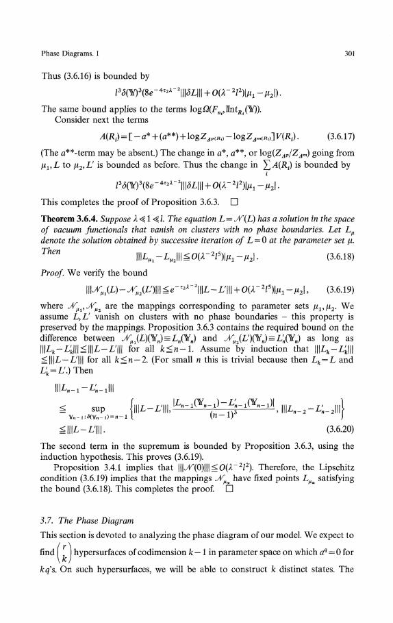
Phase Diagrams. I 301
Thus (3.6.16) is bounded by
The same bound applies to the terms logΩ(FΠί,ΠntΛ.(¥)).Consider next the terms
A(Rt) = [ - α* + (α**) + logZ^(Λ|) - logZ^*,,] V(Ri) . (3.6. 17)
(The α**-term may be absent.) The change in α*, α**, or \og(ZAP/ZAm) going from
μ1?L to μ2>^' is bounded as before. Thus the change in £^4(1 )̂ is bounded by
This completes the proof of Proposition 3.6.3. D
Theorem 3.6.4. Suppose λ <^ 1 <ζ I. The equation L = Λ^(L) has a solution in the spaceof vacuum functional^ that vanish on clusters with no phase boundaries. Let Lμ
denote the solution obtained by successive iteration of L = 0 at the parameter set μ.
Tken \\\Lμι-LJ\^0(λ-2l5)\μι-μ2\. (3.6.18)
Proof. We verify the bound
(3.6.19)
where Λ^Λ^ are the mappings corresponding to parameter sets μl9μ2. Weassume L,L' vanish on clusters with no phase boundaries - this property ispreserved by the mappings. Proposition 3.6.3 contains the required bound on thedifference between ^(L)^n) = Ln(^n] and Λ^U/XYJ = L'n(Ύn) as long asl l lLfc-Li l l l^ l l lL-L'IH for all fcgn-1. Assume by induction that |||Lk-Zi|||^|||L — L'HI for all k^n — 2. (For small n this is trivial because then Lk = L andLi = L'.) Then
sup
£\\\L-L'\\\. (3.6.20)
The second term in the supremum is bounded by Proposition 3.6.3, using theinduction hypothesis. This proves (3.6.19).
Proposition 3.4.1 implies that |||̂ (0)||| ̂ 0(λ~2l2). Therefore, the Lipschitzcondition (3.6.19) implies that the mappings ^KUα have fixed points Lμ<χ satisfyingthe bound (3.6.18). This completes the proof. D
3.7. The Phase Diagram
This section is devoted to analyzing the phase diagram of our model. We expect to
find hypersurfaces of codimension k — 1 in parameter space on which aq = 0 for\k]
kq's. On such hypersurfaces, we will be able to construct k distinct states. The
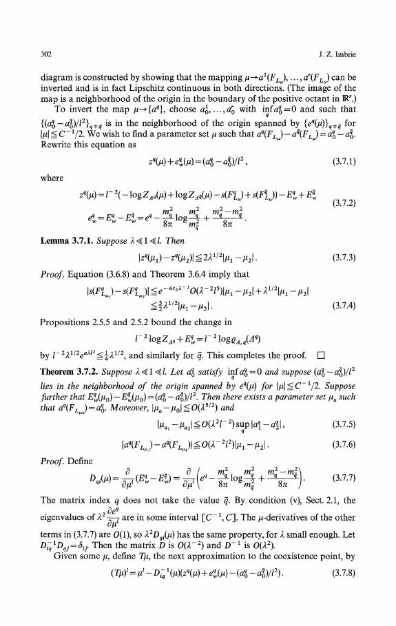
302 J. Z. Imbrie
diagram is constructed by showing that the mapping μ-^ai(FL ),..., ar(FL ) can beinverted and is in fact Lipschitz continuous in both directions. (The image of themap is a neighborhood of the origin in the boundary of the positive octant in IR1*.)
To invert the map μ-+{aq}, choose αj, ...,ar
Q with inf᧠= 0 and such that
{(#0"ao)/l2}q*q is in the neighborhood of the origin spanned by {eq(μ)}qή:q for\μ\ ̂ C~ Y2. We wish to find a parameter set μ such that aq(FLμ) - aq(FLμ) = aq
Q- d\.Rewrite this equation as
where
zq(μ) = Γ \ - \ogZΔq(μ) + logZ,,(μ) - s(Fl) + s(Fq
Lt))-Eq
w + Eq
w
e« =E
q -Eq =eq- ̂ log^ + ml'ml^w ^w ^w V Q ιυ& 2 ^ 0on m- on
Lemma 3.7.1. Suppose λ<ζl<ζl. Then
|z«(μι)-zί(μ2)l^2A1/2|μ1-μ2|. (3.7.3)
Proof. Equation (3.6.8) and Theorem 3.6.4 imply that
μ2\. (3.7.4)
Propositions 2.5.5 and 2.5.2 bound the change in
by Γ2λ1/2eaλl2^λί/2
9 and similarly for q. This completes the proof. D
Theorem 3.7.2. Suppose λ<ζl<ζl. Let a\ satisfy infαg = 0 and suppose (aqQ~a\)/l2
lies in the neighborhood of the origin spanned by eq(μ) for \μ\^C~1/2. Supposefurther that £^(μ0) — £|(μ0)
= (αo ~~ αo)/'2 Then there exists a parameter set μa suchthat aq(FLμ) = aq
0. Moreover, \μa-μ0\^0(λ5/2) and
\μaι ~ μa2\ ̂ 0(λ2Γ 2) sup \a\ -aq
2\, (3.7.5)
\aq(FLμ) - aq(FLJ ^ 0(λ~ 2l2}\μ, - μ2| . (3.7.6)
Proof. Define
The matrix index q does not take the value q. By condition (v), Sect. 2.1, thedeq
eigenvalues of ̂ 2 ̂ -7 are in some interval [C"1, C]. The //-derivatives of the other
terms in (3.7.7) are 0(1), so λ2Dqi(μ) has the same property, for λ small enough. LetD:q
ίDqj = δij. Then the matrix D is 0(λ~2) and D"1 is 0(λ2).Given some μ, define 7μ, the next approximation to the coexistence point, by
' = μ< - DΓ \μ)(zq(μ) + eq
w(μ) - (fl§ - 4)//2) . (3.7.8)
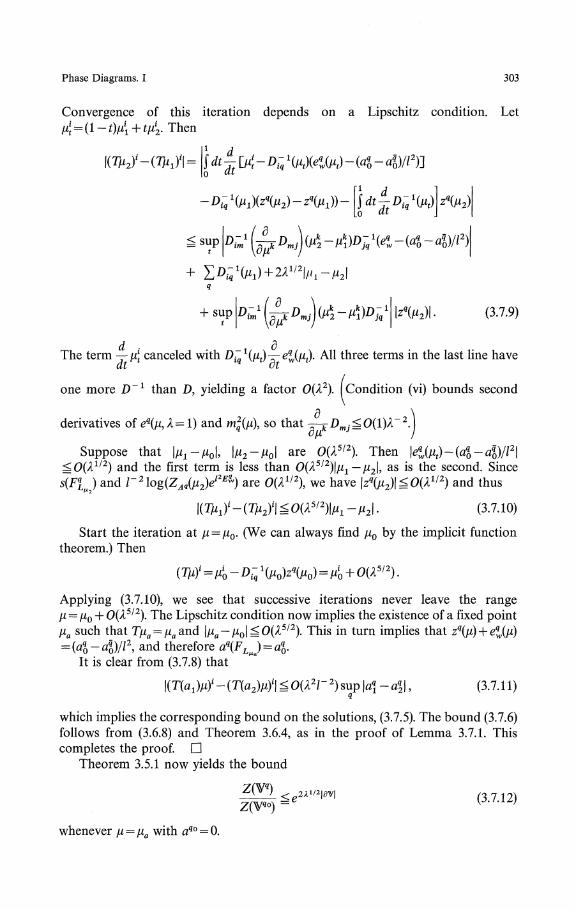
Phase Diagrams. I 303
Convergence of this iteration depends on a Lipschitz condition. Letμ\ = (l-ί)μί + t/4 Then
i(7j£2)'-(ϊϊ*ι)'i= Ulw-v
^ sup
-(αδ-4)/ί2)]
i , ί --ι.
+ sup (3.7.9)
The term — μ\ canceled with Diq
1(μt) — e^(μt). All three terms in the last line have
one more D"1 than D, yielding a factor O(λ2). Condition (vi) bounds second
derivatives of eq(μ,λ=l) and m2(μ\ so that —^Dmj^ 0(1)1 ~2.
Suppose that l^— μ0|, |μ2 — μ0| are 0(A5/ ). Then5^O(Λ1/2) and the first term is less than O(λ5/2)\μ1— μ2|, as is the second. Sinces(Fq
LJ and Γ2log(ZAq(μ2)el2E™) are 0(A1/2), we have \zq(μ2)\^0(λ1/2) and thus
Start the iteration at μ = μ0 (We can always find μ0 by the implicit functiontheorem.) Then
Applying (3.7.10), we see that successive iterations never leave the rangeμ = μ0 + 0(λ512). The Lipschitz condition now implies the existence of a fixed pointμa such that Γμα = μαand |μα-μ0|^0(A5/2). This in turn implies that zq(μ) + eq
w(μ)= (aq-aq
0)/l2, and therefore aq(FLJ = aq
0.It is clear from (3.7.8) that
2 2 )sup|αj-α||, (3.7.11)
which implies the corresponding bound on the solutions, (3.7.5). The bound (3.7.6)follows from (3.6.8) and Theorem 3.6.4, as in the proof of Lemma 3.7.1. Thiscompletes the proof. D
Theorem 3.5.1 now yields the bound
(3.7.12)
whenever μ = μα with αg° = 0.
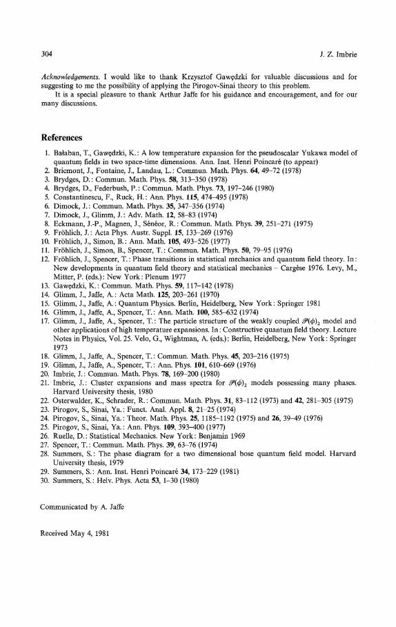
304 J. Z. Imbrie
Acknowledgements. I would like to thank Krzysztof Gawζdzki for valuable discussions and forsuggesting to me the possibility of applying the Pirogov-Sinai theory to this problem.
It is a special pleasure to thank Arthur Jaffe for his guidance and encouragement, and for ourmany discussions.
References
1. Balaban, T., Gawedzki, K.: A low temperature expansion for the pseudoscalar Yukawa model ofquantum fields in two space-time dimensions. Ann. Inst. Henri Poincare (to appear)
2. Bricmont, J., Fontaine, J., Landau, L.: Commun. Math. Phys. 64, 49-72 (1978)3. Brydges, D.: Commun. Math. Phys. 58, 313-350 (1978)4. Brydges, D., Federbush, P.: Commun. Math. Phys. 73, 197-246 (1980)5. Constantinescu, F., Ruck, H.: Ann. Phys. 115, 474-495 (1978)6. Dimock, J.: Commun. Math. Phys. 35, 347-356 (1974)7. Dimock, J., Glimm, J.: Adv. Math. 12, 58-83 (1974)8. Eckmann, J.-P., Magnen, J., Seneor, R.: Commun. Math. Phys. 39, 251-271 (1975)9. Frohlich, J.: Acta Phys. Austr. Suppl. 15, 133-269 (1976)
10. Frohlich, J., Simon, B.: Ann. Math. 105, 493-526 (1977)11. Frohlich, J., Simon, B., Spencer, T.: Commun. Math. Phys. 50, 79-95 (1976)12. Frohlich, J., Spencer, T.: Phase transitions in statistical mechanics and quantum field theory. In:
New developments in quantum field theory and statistical mechanics - Cargese 1976. Levy, M.,Mitter, P. (eds.): New York: Plenum 1977
13. Gawedzki, K.: Commun. Math. Phys. 59, 117-142 (1978)14. Glimm, J., Jaffe, A.: Acta Math. 125, 203-261 (1970)15. Glimm, J., Jaffe, A.: Quantum Physics. Berlin, Heidelberg, New York: Springer 198116. Glimm, J., Jaffe, A., Spencer, T.: Ann. Math. 100, 585-632 (1974)17. Glimm, J., Jaffe, A., Spencer, T.: The particle structure of the weakly coupled 0>(φ)2 model and
other applications of high temperature expansions. In: Constructive quantum field theory. LectureNotes in Physics, Vol. 25. Velo, G., Wightman, A. (eds.): Berlin, Heidelberg, New York: Springer1973
18. Glimm, J., Jaffe, A., Spencer, T.: Commun. Math. Phys. 45, 203-216 (1975)19. Glimm, J., Jaffe, A., Spencer, T.: Ann. Phys. 101, 610-669 (1976)20. Imbrie, J.: Commun. Math. Phys. 78, 169-200 (1980)21. Imbrie, J.: Cluster expansions and mass spectra for ^(φ)2 models possessing many phases.
Harvard University thesis, 198022. Osterwalder, K., Schrader, R.: Commun. Math. Phys. 31, 83-112 (1973) and 42, 281-305 (1975)23. Pirogov, S., Sinai, Ya.: Funct. Anal. Appl. 8, 21-25 (1974)24. Pirogov, S, Sinai, Ya.: Theor. Math. Phys. 25, 1185-1192 (1975) and 26, 39-49 (1976)25. Pirogov, S., Sinai, Ya.: Ann. Phys. 109, 393-400 (1977)26. Ruelle, D.: Statistical Mechanics. New York: Benjamin 196927. Spencer, T.: Commun. Math. Phys. 39, 63-76 (1974)28. Summers, S.: The phase diagram for a two dimensional bose quantum field model. Harvard
University thesis, 197929. Summers, S.: Ann. Inst. Henri Poincare 34, 173-229 (1981)30. Summers, S.: Helv. Phys. Acta 53, 1-30 (1980)
Communicated by A. Jaffe
Received May 4, 1981