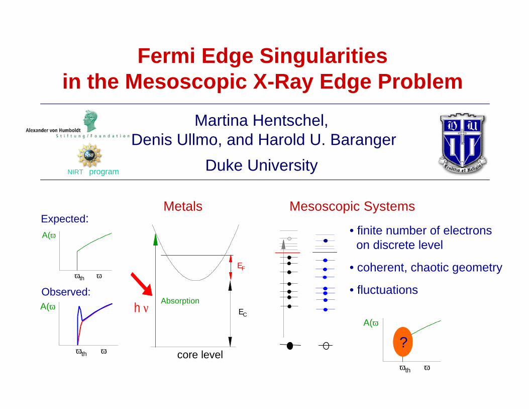
Metals Mesoscopic SystemsExpected:A(ω)

ωth ω

A(ω)

ωth ω

Observed:

core level

{ε}

EF

EC

Absorptionh ν

Fermi Edge Singularities in the Mesoscopic X-Ray Edge Problem

Martina Hentschel,Denis Ullmo, and Harold U. Baranger

Duke University

• finite number of electrons on discrete level

• coherent, chaotic geometry

• fluctuations

{λ}

NIRT program

A(ω)

ωth ω

?

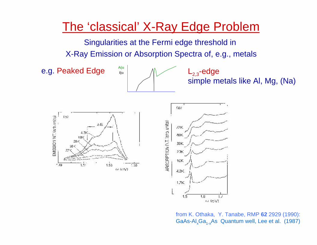
e.g. Peaked Edge L2,3-edgesimple metals like Al, Mg, (Na)

from K. Othaka, Y. Tanabe, RMP 62 2929 (1990):GaAs-AlxGa1-xAs Quantum well, Lee et al. (1987)

A(ω)I(ω)

The ‘classical’ X-Ray Edge ProblemSingularities at the Fermi edge threshold in

X-Ray Emission or Absorption Spectra of, e.g., metals

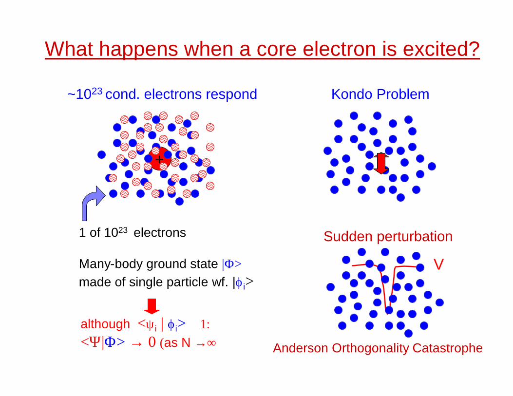
although <ψi | ϕi> ∼ 1:<Ψ|Φ> → 0 (as N →∞)

+

1 of 1023 electrons

Many-body ground state |Φ>made of single particle wf. |ϕi>

What happens when a core electron is excited?

~1023 cond. electrons respond Kondo Problem

V

Sudden perturbation

Anderson Orthogonality Catastrophe

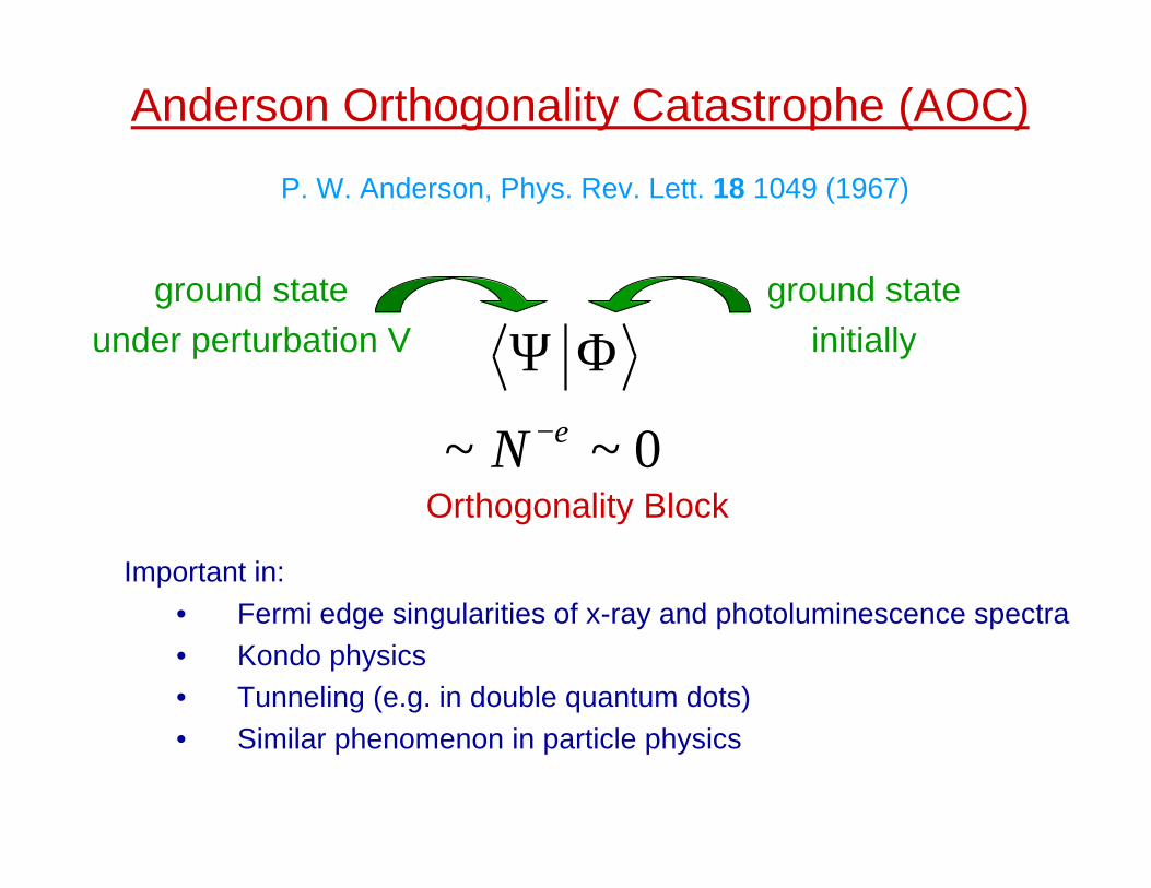
Anderson Orthogonality Catastrophe (AOC)

P. W. Anderson, Phys. Rev. Lett. 18 1049 (1967)

0~~ ε−

ΦΨ

N

Important in:• Fermi edge singularities of x-ray and photoluminescence spectra• Kondo physics• Tunneling (e.g. in double quantum dots)• Similar phenomenon in particle physics

ground stateinitially

ground stateunder perturbation V

Orthogonality Block

screeningdipole selection rules

Orthogonality blockdue to AOC

Peaked or rounded edge ?

Many-body effect“Mahan’s enhancement”

Competition

acts universal

finite Nfinite N

chaotic geometry relative strength ?

Mesoscopic effects

Sample-to-sample fluctuations

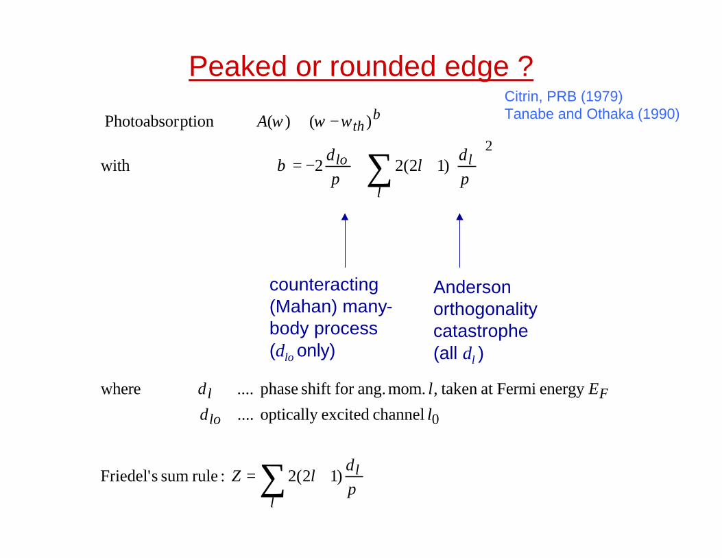
Peaked or rounded edge ?

∑

∑

+=

++−=

−∝

l

l

lo

Fl

l

l

lo

th

lZ

l

El

l

A

πδ

δ

δ

πδ

πδ

β

ωωω β

)12(2 :rule sum sFriedel'

channel excitedoptically ....

energy Fermiat taken , mom. ang.for shift phase .... where

)12(22 with

)()( ption Photoabsor

0

2

Anderson orthogonality catastrophe(all δl )

counteracting(Mahan) many-body process (δlo only)

Citrin, PRB (1979)Tanabe and Othaka (1990)

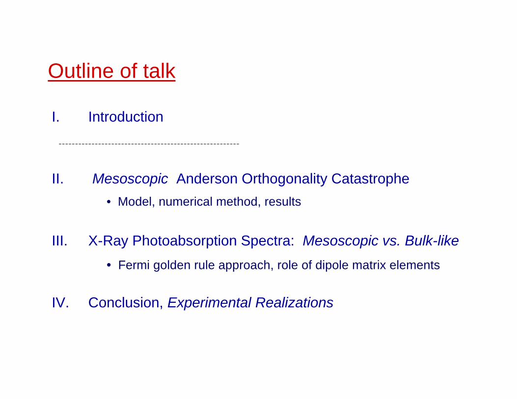
I. Introduction

II. Mesoscopic Anderson Orthogonality Catastrophe

III. X-Ray Photoabsorption Spectra: Mesoscopic vs. Bulk-like

IV. Conclusion, Experimental Realizations

Outline of talk

• Model, numerical method, results

• Fermi golden rule approach, role of dipole matrix elements

II. Anderson Orthogonality Catastrophe

in Mesoscopic Systems

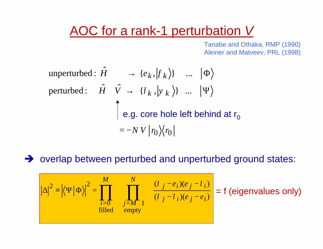
AOC for a rank-1 perturbation VTanabe and Othaka, RMP (1990)Aleiner and Matveev, PRL (1998)

Ψ→+

Φ→

...},{ˆˆ :perturbed

...},{ˆ :dunperturbe

κκ ψλ

φε

VH

H kk

∏ ∏= +=

−−

−−=ΦΨ≡∆

M

i

N

Mj ijij

ijij

filled0

empty

1

22

))((

))((

εελλ

λεελ= f (eigenvalues only)

00 rrVN−=

e.g. core hole left behind at r0

è overlap between perturbed and unperturbed ground states:

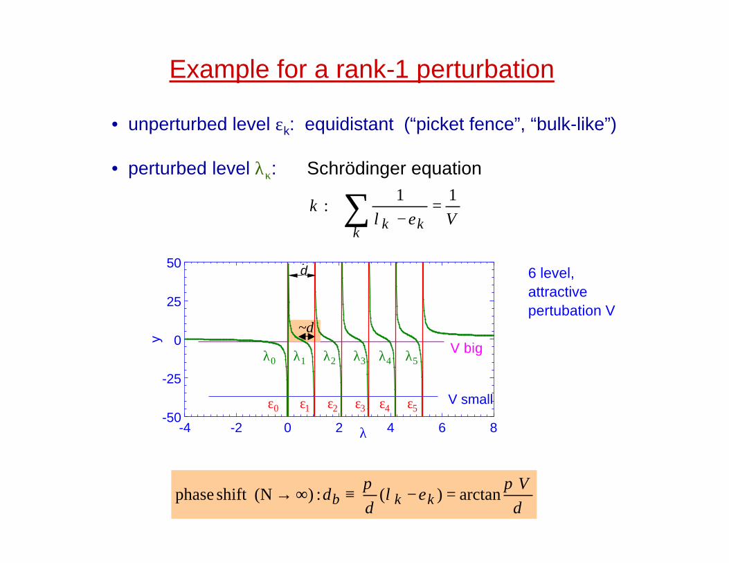
• unperturbed level εk: equidistant (“picket fence”, “bulk-like”)

• perturbed level λκ: Schrödinger equation

Example for a rank-1 perturbation

Vk k

11: =

−∀ ∑ ελ

κκ

λ0 λ1 λ2 λ3 λ4 λ5 V big

V small

dV

d kkbπ

ελπ

δ arctan)(:) (Nshift phase =−≡∞→

∼δ

-4 -2 0 2 4 6 8λ-50

-25

0

25

50

y

6 level, attractive pertubation V

ε0 ε1 ε2 ε3 ε4 ε5

∆d

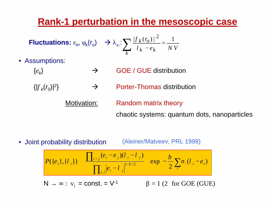
• Assumptions:{εk} à GOE / GUE distribution

{|φk(r0)|2} à Porter-Thomas distribution

Motivation: Random matrix theory

chaotic systems: quantum dots, nanoparticles

• Joint probability distribution

N → ∞ : νi = const. = V-1 β = 1 (2) for GOE (GUE)

(Aleiner/Matveev, PRL 1998)

−−

−

−−∝ ∑

∏∏

−>

iii

ji ji

ji jiji

ii iP )(

2exp

))((}){},({

,

2/1 ελνβ

λε

λλεελε β

Rank-1 perturbation in the mesoscopic case

VNr

k k

ok 1|)(| 2=

−∑ ελφ

κFluctuations: εk, φk(ro) à λκ::

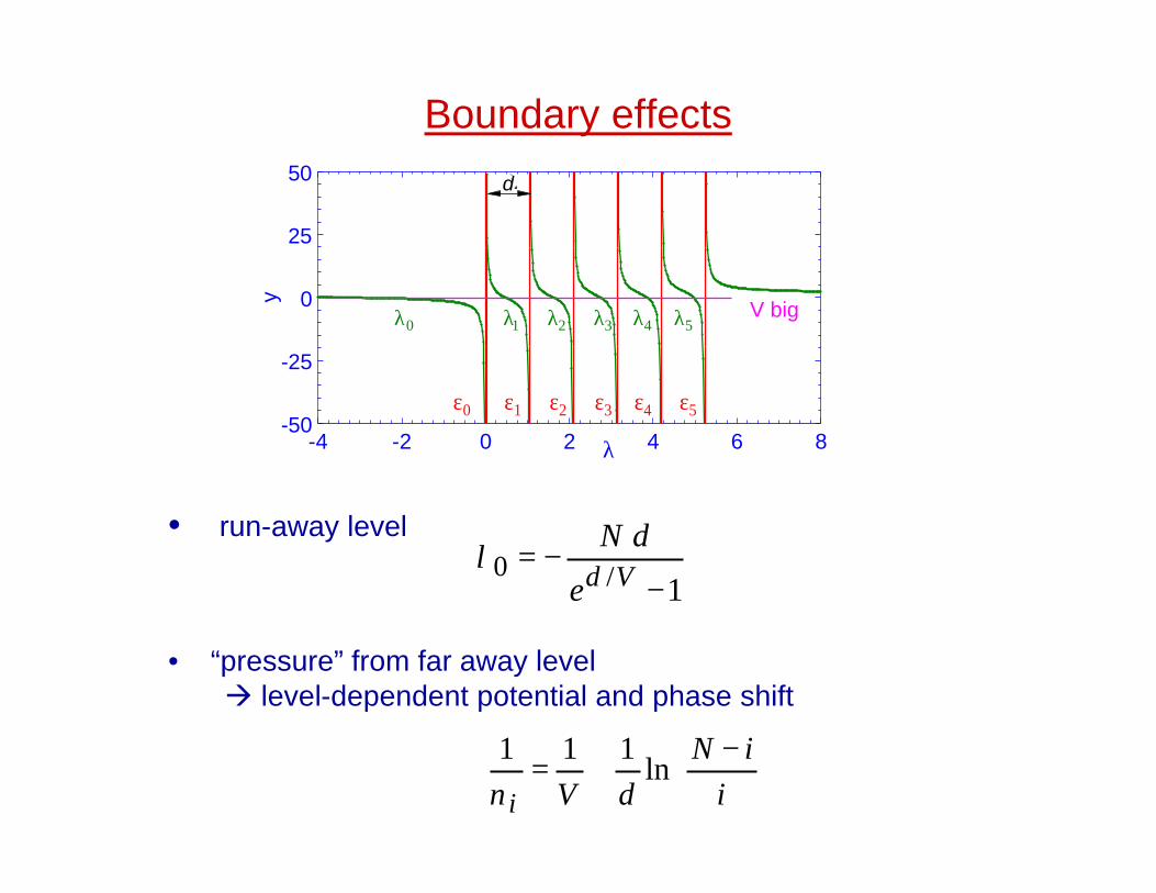
Boundary effects

• run-away level

• “pressure” from far away level à level-dependent potential and phase shift

1/0−

−=Vde

dNλ

−+=

iiN

dViln

111ν

-4 -2 0 2 4 6 8λ-50

-25

0

25

50

y

ε0 ε1 ε2 ε3 ε4 ε5

∆

λ0 λ1 λ2 λ3 λ4 λ5 V big

d

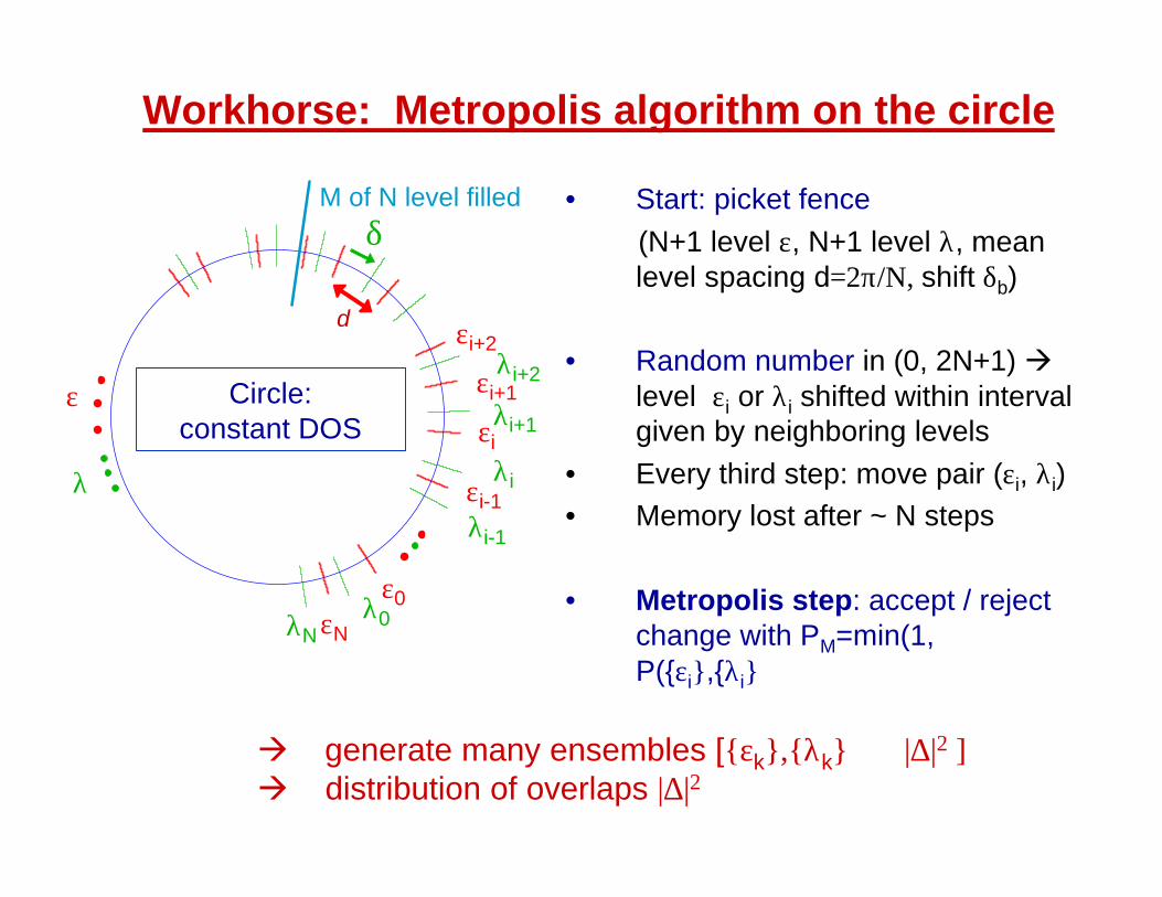
Workhorse: Metropolis algorithm on the circle

• Start: picket fence (N+1 level ε, N+1 level λ, mean level spacing d=2π/Ν, shift δb)

• Random number in (0, 2N+1) àlevel εi or λi shifted within interval given by neighboring levels

• Every third step: move pair (εi, λi)• Memory lost after ~ N steps

• Metropolis step: accept / reject change with PM=min(1, P({εi},{λi}))

εi

εi+1

εi+2

εi-1λi

λi+2

λi+1

λi-1

ε

λ

δ

∆

εNλ0λN

ε0

M of N level filled

à generate many ensembles [{εk},{λk} ⇒ |∆|2 ]à distribution of overlaps |∆|2

Circle:constant DOS

d

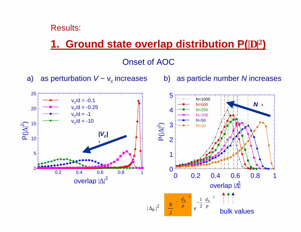
Results:

1. Ground state overlap distribution P(|∆|2)

a) as perturbation V ~ vc increases b) as particle number N increases

0.2 0.4 0.6 0.8 1

overlap |∆|20

5

10

15

20

25

P(|∆

|2 )

vc/d = -0.1vc/d = -0.25vc/d = -1vc/d = -10

Onset of AOC

0 0.2 0.4 0.6 0.8 1overlap |∆|2

0

1

2

3

4

5

P(|∆

|2 )

N=1000N=500N=250N=100N=50N=10

bulk values

22

21

22

||

−

−

∝∆ π

δπδ bb

eN

b

|Vc|↑

N ↑

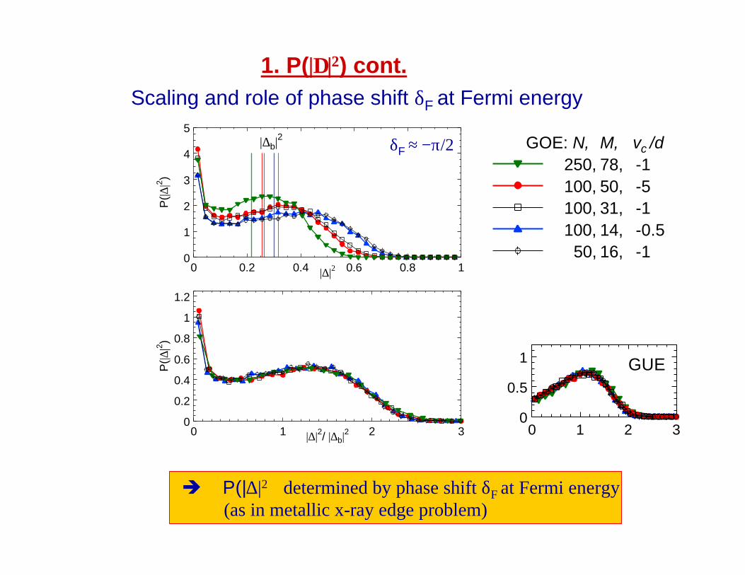
è P(|∆|2) determined by phase shift δF at Fermi energy(as in metallic x-ray edge problem)

0 0.2 0.4 0.6 0.8 1|∆|20

1

2

3

4

5

P(|∆

|2 )

GOE: N, M, vc /d250, 78, -1100, 50, -5100, 31, -1100, 14, -0.5 50, 16, -1

|∆b|2

0 1 2 3|∆|2/ |∆b|20

0.2

0.4

0.6

0.8

1

1.2

P(|∆

|2 )

0 1 2 30

0.5

1 GUE

Scaling and role of phase shift δF at Fermi energy

δF ≈ −π/2

1. P(|∆|2) cont.

Results:

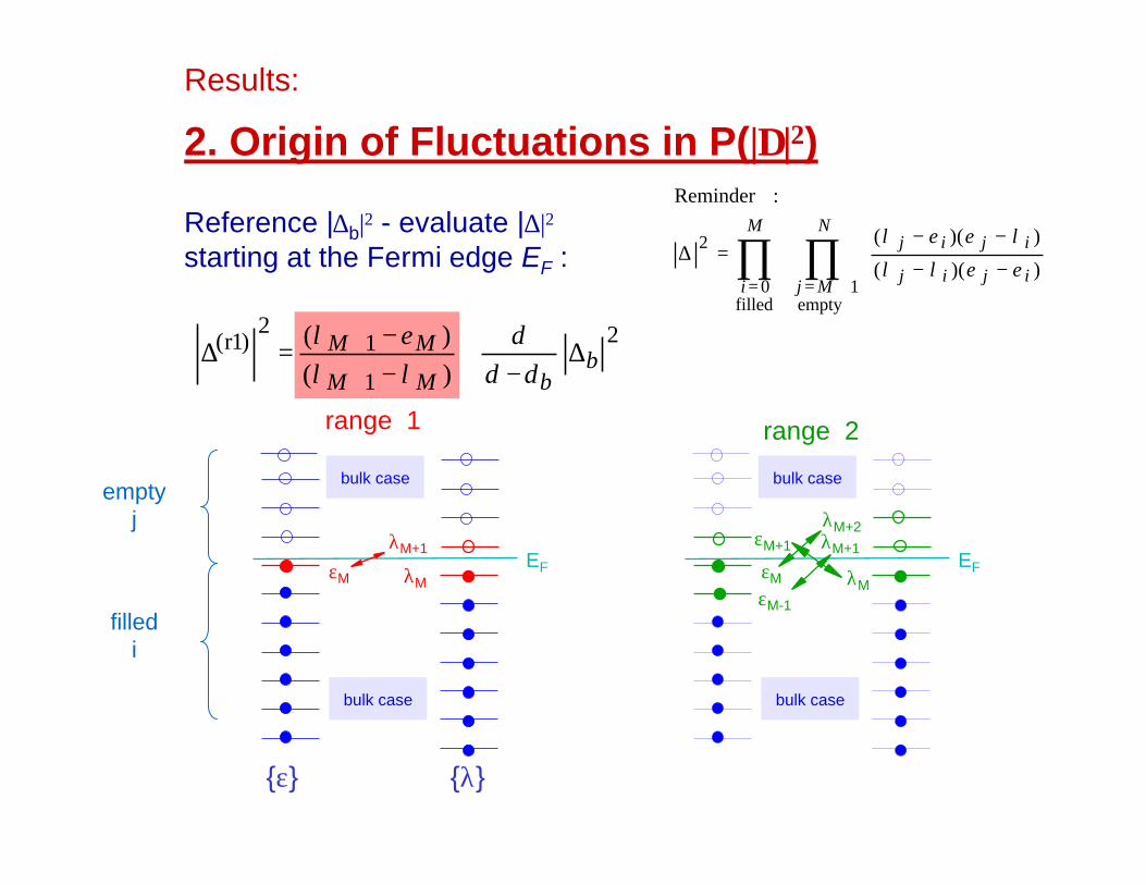
2. Origin of Fluctuations in P(|∆|2)

∏ ∏= +=

−−

−−=∆

M

i

N

Mj ijij

ijij

filled0

empty 1

2

))((

))((

:Reminder

εελλ

λεελReference |∆b|2 - evaluate |∆|2

starting at the Fermi edge EF :

{ε} {λ}

EF

λM+1

εM

bulk case

bulk case

λM

range 2

EF

λM+1

εM

bulk case

bulk case

εM+1

λM

λM+2

εM-1

range 1

emptyj

filledi

2

1

12

)1r()()(

bbMM

MMd

d∆

−−−

=∆+

+δλλ

ελ

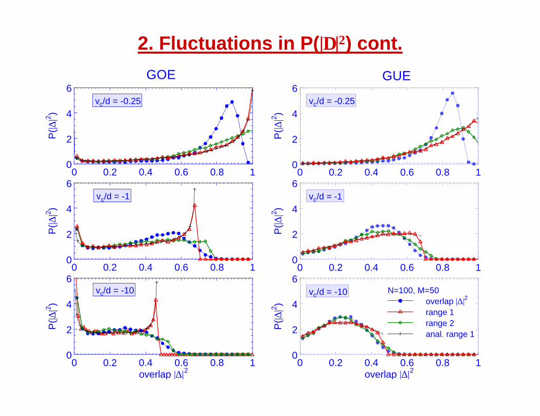
2. Fluctuations in P(|∆|2) cont.

0 0.2 0.4 0.6 0.8 10

2

4

6

P(|∆

|2 )

vc/d = -1

0 0.2 0.4 0.6 0.8 10

2

4

6

P(|∆

|2 )

vc/d = -0.25

0 0.2 0.4 0.6 0.8 1overlap |∆|2

0

2

4

6P

(|∆|2 )

vc/d = -10

GUE

0 0.2 0.4 0.6 0.8 10

2

4

6

P(|∆

|2 )

GOE

vc/d = -1

0 0.2 0.4 0.6 0.8 10

2

4

6

P(|∆

|2 )

vc/d = -0.25

0 0.2 0.4 0.6 0.8 1overlap |∆|2

0

2

4

6

P(|∆

|2 )

vc/d = -10 N=100, M=50overlap |∆|2

range 1range 2anal. range 1

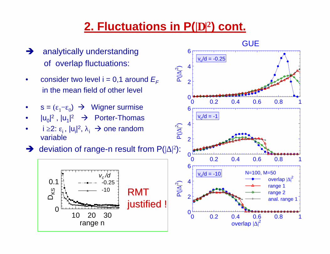
10 20 30range n

0

0.1

DK

S

è deviation of range-n result from P(|∆|2):

vc /d-0.25-10

2. Fluctuations in P(|∆|2) cont.

è analytically understandingof overlap fluctuations:

• consider two level i = 0,1 around EF

in the mean field of other level

• s = (ε1−ε0) à Wigner surmise• |u0|2 , |u1|2 à Porter-Thomas • i ≥2: εi , |ui|2, λi à one random

variable

RMTRMTjustified !justified !

0 0.2 0.4 0.6 0.8 10

2

4

6

P(|∆

|2 )

vc/d = -1

0 0.2 0.4 0.6 0.8 10

2

4

6

P(|∆

|2 )

vc/d = -0.25

0 0.2 0.4 0.6 0.8 1overlap |∆|2

0

2

4

6

P(|∆

|2 )vc/d = -10

GUE

N=100, M=50overlap |∆|2

range 1range 2anal. range 1

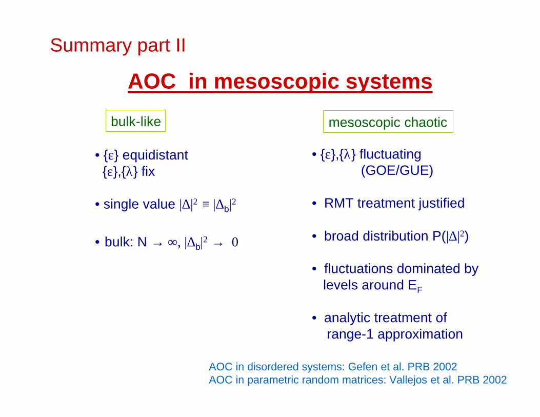
Summary part II

AOC in mesoscopic systems

bulk-like mesoscopic chaotic

• {ε} equidistant{ε},{λ} fix

• single value |∆|2 ≡ |∆b|2

• bulk: N → ∞, |∆b|2 → 0

• {ε},{λ} fluctuating (GOE/GUE)

• RMT treatment justified

• broad distribution P(|∆|2)

• fluctuations dominated by levels around EF

• analytic treatment of range-1 approximation

AOC in disordered systems: Gefen et al. PRB 2002AOC in parametric random matrices: Vallejos et al. PRB 2002

III. Mesoscopic X-ray Edge Problem

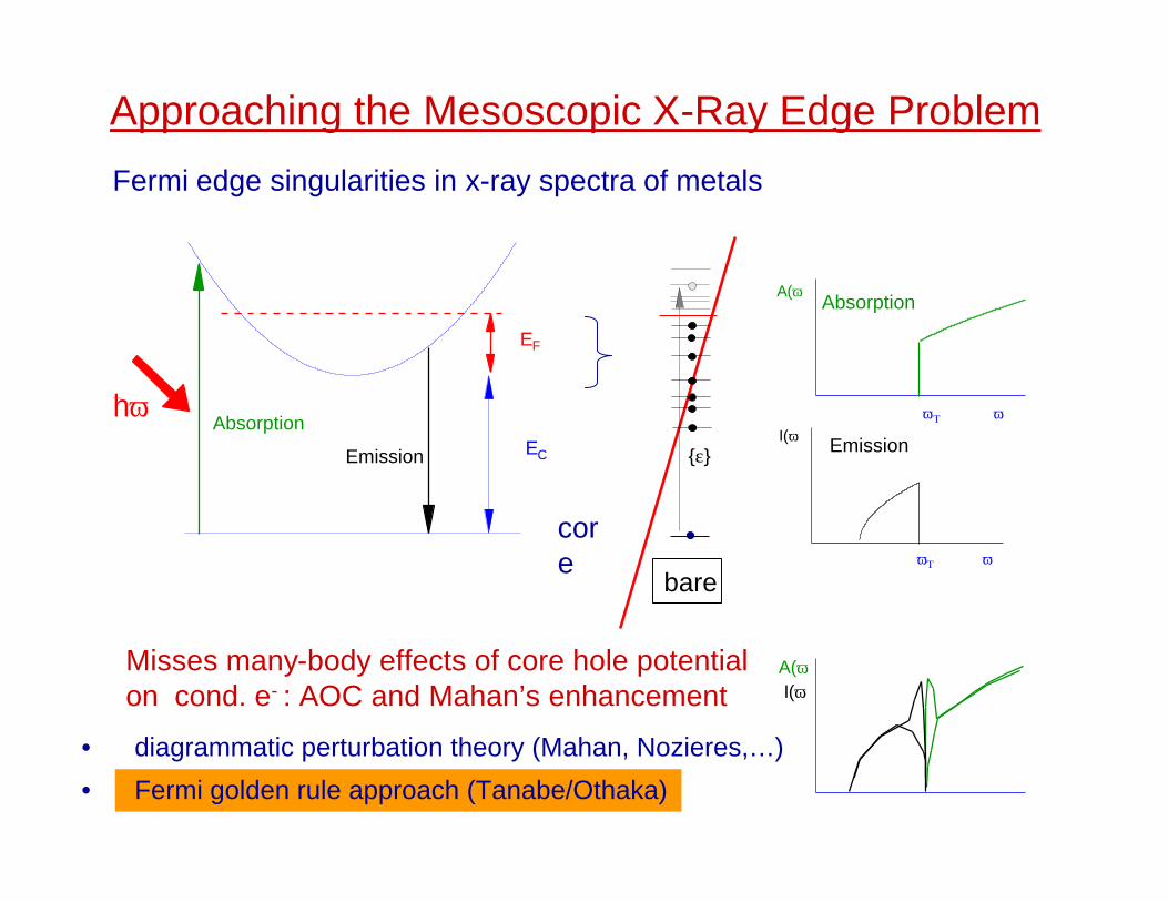
Approaching the Mesoscopic X-Ray Edge Problem

Fermi edge singularities in x-ray spectra of metals

EF

EC

Absorption

Emission

h___ ω

AbsorptionA(ω)

ωΤ ω

EmissionI(ω)

ωΤ ω

A(ω)I(ω)

core

Misses many-body effects of core hole potentialon cond. e- : AOC and Mahan’s enhancement

• diagrammatic perturbation theory (Mahan, Nozieres,…)

• Fermi golden rule approach (Tanabe/Othaka)

bare

{ε}

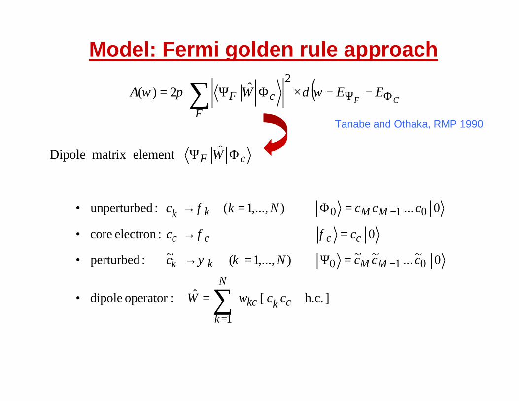
Model: Fermi golden rule approach

( )CF

EEWA

FcF ΦΨ −−×ΦΨ= ∑ ωδπω

2ˆ2)(

] h.c.[ˆ :operator dipole

0~...~~ ),...,1( ~ : perturbed

0 :electron core

0... ),...,1( : dunperturbe

1

010

010

+=•

=Ψ=→•

=→•

=Φ=→•

∑=

+

++−

++

++

++−

++

N

kckkc

MM

cccc

MMkk

ccwW

cccNc

cc

cccNkc

κψ

φφ

φ

κκ

cF W ΦΨ ˆelement matrix Dipole

Tanabe and Othaka, RMP 1990

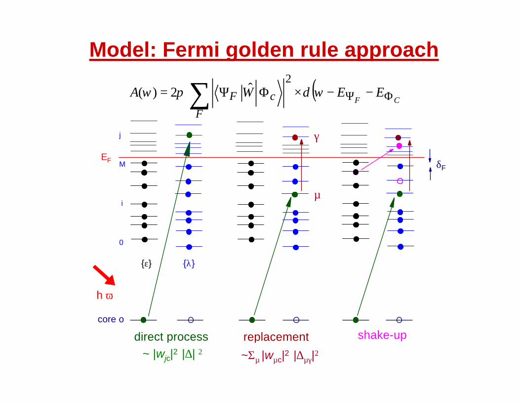
Model: Fermi golden rule approach

( )CF

EEWA

FcF ΦΨ −−×ΦΨ= ∑ ωδπω

2ˆ2)(

direct process replacement shake-updirect

EF

core o

j

M

i

0

{ε}

δF

h___ ω

{λ}

~ |wjc|2 |∆| 2 ~Σµ |wµc|2 |∆µγ|2

µ

γ

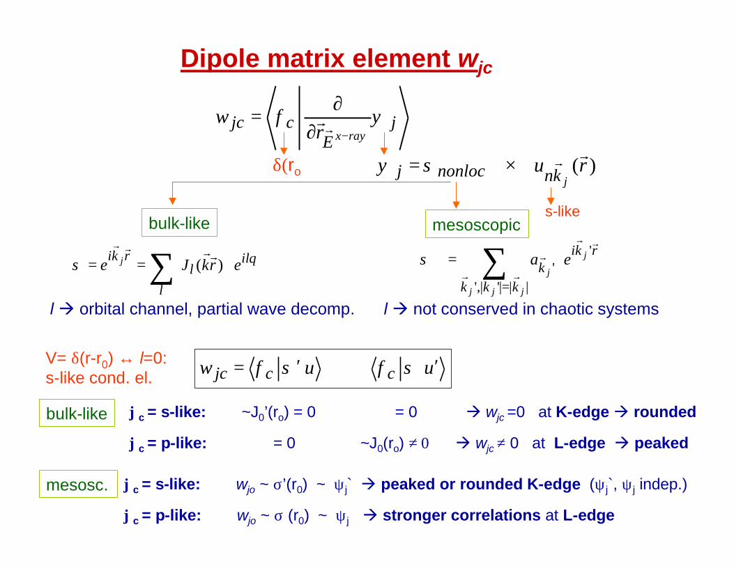
Dipole matrix element wjc

jE

cjcrayxr

w ψφ−∂

∂= rr

ufufw ccjc ′+′= σσ

)( rujknnonlocj

rr×= σψ∼δ(ro)

s-likebulk-like mesoscopic

θσ il

ll

rkierkJe j ∑== )(

rrrr

∑=

=

||'||,'

''

jjj

j

j

kkk

rkik ea

rrr

rrrσ

là orbital channel, partial wave decomp. là not conserved in chaotic systems

ϕc = s-like: ~J0’(ro) = 0 = 0 à wjc =0 at K-edge à rounded

ϕc = p-like: = 0 ~J0(ro) ≠ 0 à wjc ≠ 0 at L-edge à peaked

bulk-like

V= δ(r-r0) ↔ l=0: s-like cond. el.

mesosc. ϕc = s-like: wjo ~ σ’(r0) ~ ψj` à peaked or rounded K-edge (ψj`, ψj indep.)

ϕc = p-like: wjo ~ σ (r0) ~ ψj à stronger correlations at L-edge

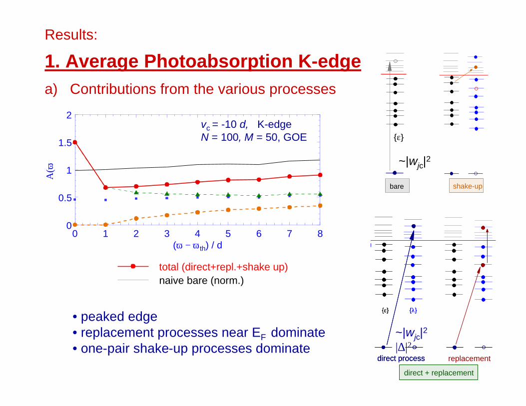
Results:

1. Average Photoabsorption K-edgea) Contributions from the various processes

T

total (direct+repl.+shake up)naive bare (norm.)

direct process

M

{ε} {λ}

shake-up

direct process replacement

M

{ε} {λ}

direct + replacement

0 1 2 3 4 5 6 7 8(ω − ωth) / d

0

0.5

1

1.5

2

⟨Α(ω

)⟩

{ε}

bare

~|wjc|2

~|wjc|2

|∆|2

vc = -10 d, K-edgeN = 100, M = 50, GOE

• peaked edge • replacement processes near EF dominate • one-pair shake-up processes dominate

Results:1. Average Photoabsorption K-edgeb) Taking spin into account

vc = -10 d, K-edgeN = 100, M = 50, GOE

spectator spin

EF

à width of |Φ0⟩in basis of perturbedfinal states |ΨF⟩

active spin

EF

active

spectator

full spin

0 1 2 3 4 5 6 7 8(ω − ωth) / d

0

0.5

1

1.5

2

⟨Α(ω

)⟩

0 1 2 3 4 5 6 7 8(ω − ωth) / d

0.1

0.3

1

3

⟨Α(ω

)⟩

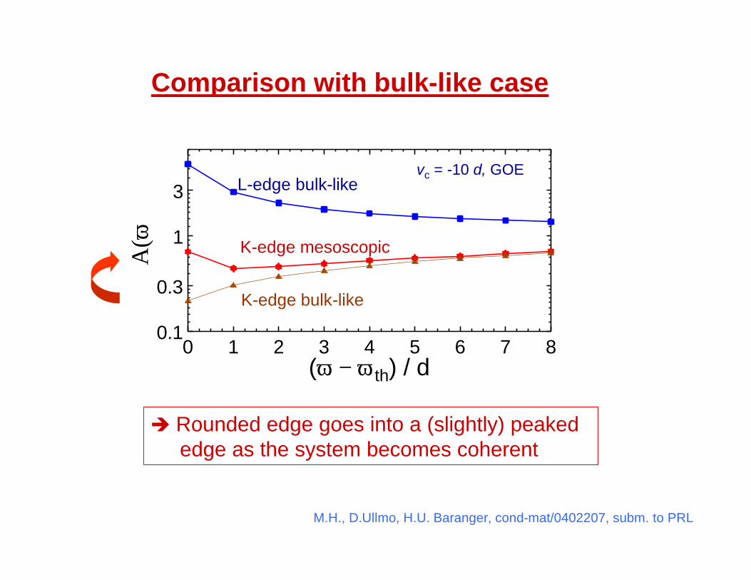
Comparison with bulk-like case

vc = -10 d, GOE

è Rounded edge goes into a (slightly) peaked edge as the system becomes coherent

M.H., D.Ullmo, H.U. Baranger, cond-mat/0402207, subm. to PRL

K-edge bulk-like

K-edge mesoscopic

L-edge bulk-like

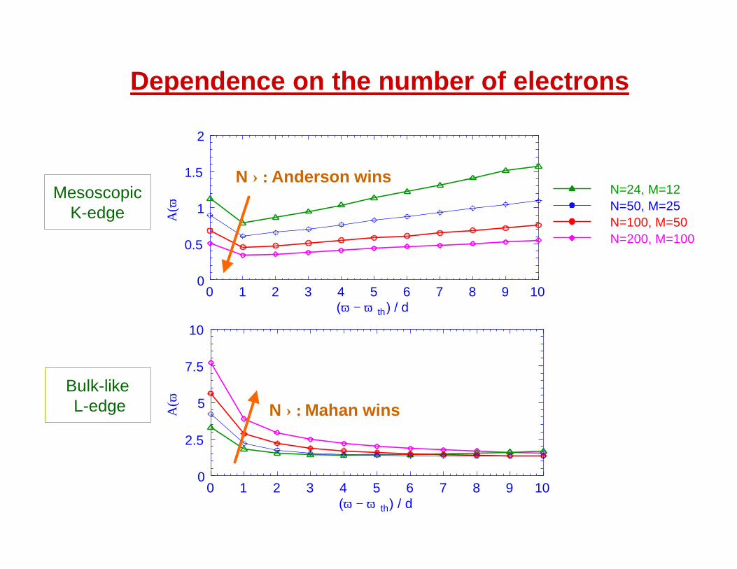
Dependence on the number of electrons

bareN=24, M=12N=50, M=25N=100, M=50N=200, M=100

MesoscopicK-edge

0 1 2 3 4 5 6 7 8 9 10(ω − ω th) / d

0

2.5

5

7.5

10

⟨Α(ω

)⟩Bulk-likeL-edge

0 1 2 3 4 5 6 7 8 9 10(ω − ω th) / d

0

0.5

1

1.5

2

⟨Α(ω

)⟩N ↑: Anderson wins

N ↑: Mahan wins

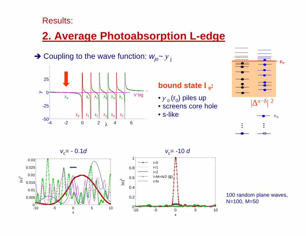
|∆π−δ| 2

EF

λ0

Results:

2. Average Photoabsorption L-edge

è Coupling to the wave function: wjo~ ψj

-4 -2 0 2 4 6λ-50

-25

0

25

y

ε0 ε1 ε2 ε3 ε4 ε5

λ0 λ1 λ2 λ3 λ4 λ5 V big

bound state λ0:

• ψ0 (r0) piles up• screens core hole• s-like

-10 -5 0 5 10x

0

0.005

0.01

0.015

0.02

0.025

0.03

|ψi|2

-10 -5 0 5 10x

0

0.2

0.4

0.6

0.8

1

|ψi|2

i=0i=1i=2i=M=N/2 (EF)i=N

vc= - 0.1d vc= -10 d

100 random plane waves, N=100, M=50

0 1 2 3 4 5 6 7 8 9 10<ω−ωth>/d

0

10

20

30

40

<A(ω

)>

0 1 2 3 4 5 6 7 8 9 10<ω−ωth>/d

0

10

20

30

40

<A(ω

)>

N=100, M=50N=50, M=25

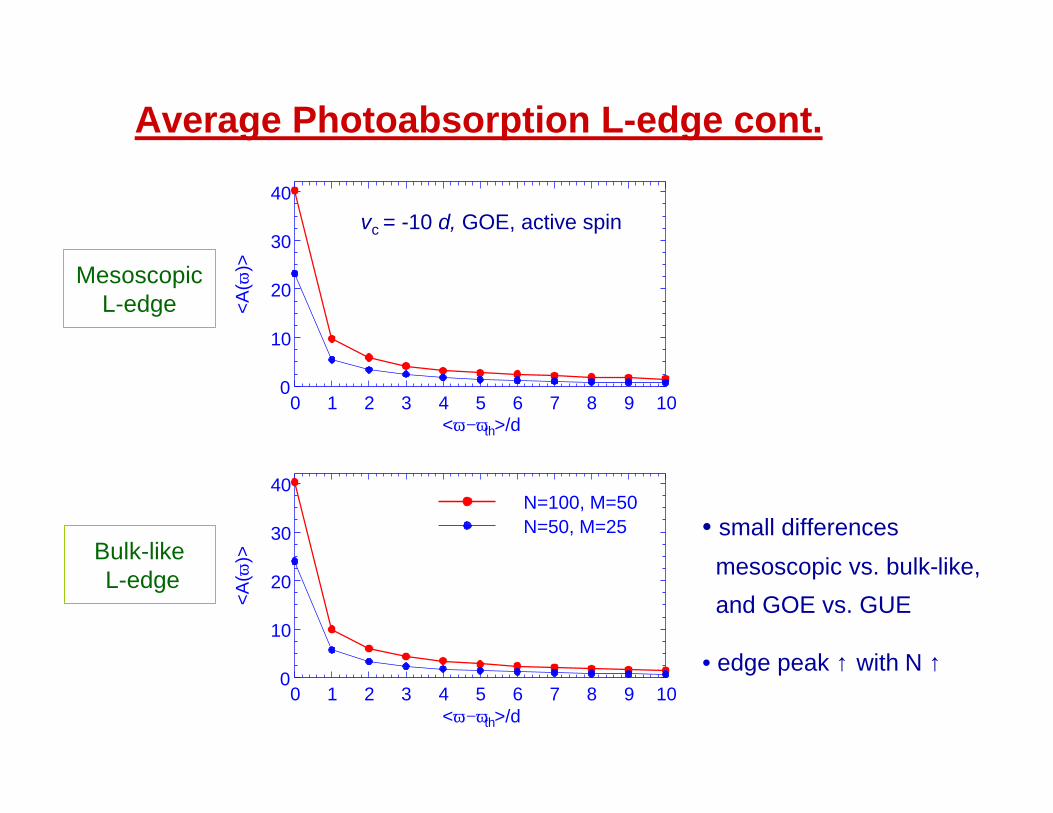
vc = -10 d, GOE, active spin

• small differences

mesoscopic vs. bulk-like,

and GOE vs. GUE

• edge peak ↑ with N ↑

Average Photoabsorption L-edge cont.

MesoscopicL-edge

Bulk-likeL-edge

0 1 2 3 4A(ω) / <A(ω)>

0

0.5

1

1.5

2

P(A

(ω)

/ <A

(ω)>

)

0 1 2 3 4A(ω) / <A(ω)>

0

0.5

1

1.5

2

P(A

(ω)

/ <A

(ω)>

)

Results:

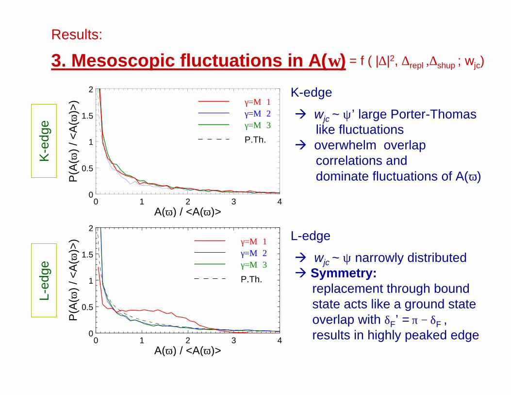
3. Mesoscopic fluctuations in A(ω)

K-edge

à wjc ~ ψ’ large Porter-Thomaslike fluctuations

à overwhelm overlap correlations anddominate fluctuations of A(ω)

γ=Μ+1γ=Μ+2γ=Μ+3γ=Μ+8P.Th.

L-edge

à wjc ~ ψ narrowly distributedà Symmetry:

replacement through bound state acts like a ground state overlap with δF’ = π − δF ,results in highly peaked edge

= f ( |∆|2, ∆repl ,∆shup ; wjc)

γ=Μ+1γ=Μ+2γ=Μ+3γ=Μ+8P.Th.

K-e

dge

L-ed

ge

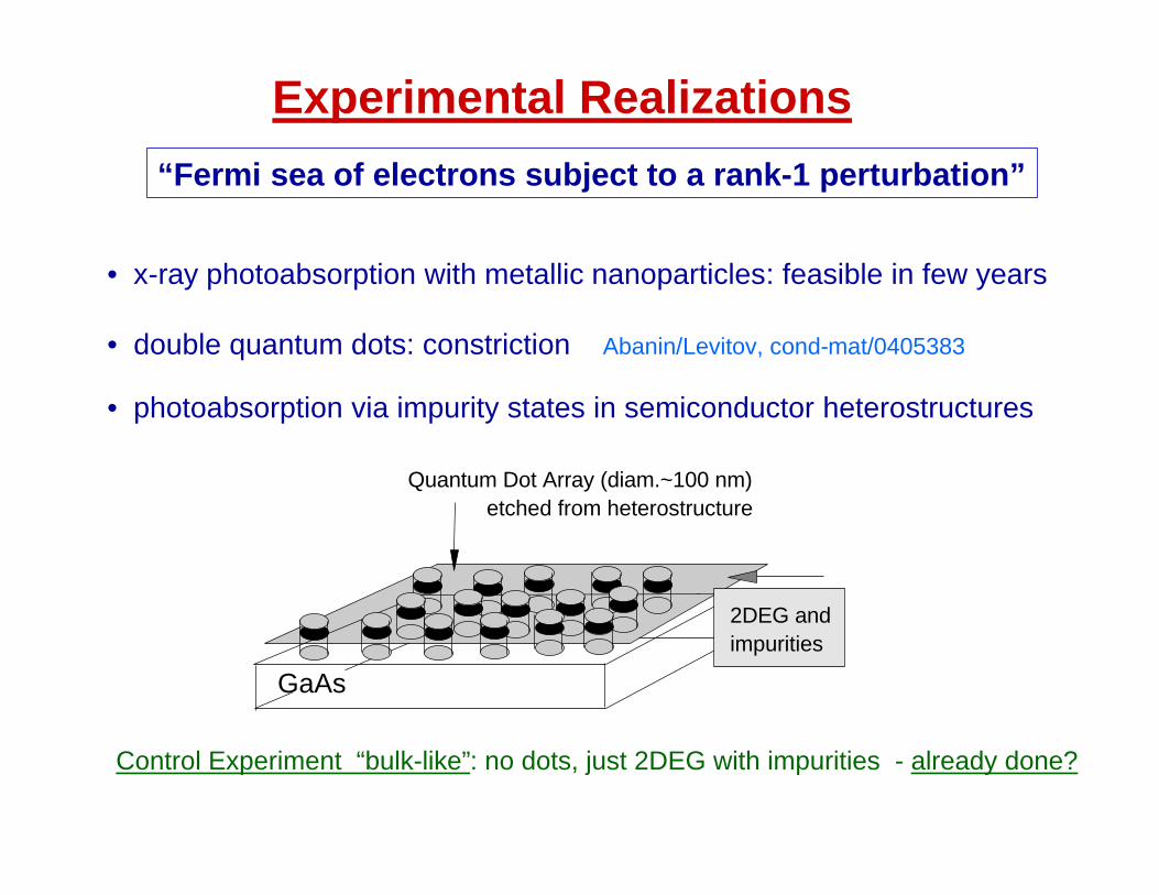
• x-ray photoabsorption with metallic nanoparticles: feasible in few years

• double quantum dots: constriction Abanin/Levitov, cond-mat/0405383

• photoabsorption via impurity states in semiconductor heterostructures

Experimental Realizations

“Fermi sea of electrons subject to a rank-1 perturbation”

GaAs

2DEG andimpurities

Quantum Dot Array (diam.~100 nm)etched from heterostructure

Control Experiment “bulk-like”: no dots, just 2DEG with impurities - already done?

Summary part III

Mesoscopic X-ray Edge Problem

bulk-like mesoscopic

s-like conduction electrons: δ0= π/2, δ1= 0

Dipole coupling changed because mesoscopic system is

- chaotic (loose l as quantum number)- coherent confinement- wave function and derivative independent

• rounded K-edge

• peaked L-edge

• (slightly) peaked K-edge

• peaked L-edgeAverage ⟨A(ω)⟩

Mesoscopic fluctuations• individual spectra can even zig-zag

IV. Conclusions• AOC in Mesoscopic Systems:

- broad distribution P(|∆|2)- scaling with |∆b|2, δF

• Mesoscopic Photoabsorption Spectra and X-Ray Edge Problem:

- K-edge: ⟨A(ω)⟩ from rounded to peaked as system becomes coherent,Porter-Thomas fluctuations

- L-edge: strongly peaked, same fluctuations as |∆|2

• Experimental realizations: - array of quantum dots, impurity level takes role of core electron

- nanoparticles, double dots M. Hentschel, D. Ullmo, H.U. Baranger,cond-mat/0402207

0 1 2 3 4 5 6 7 8(ω − ωth) / d

0.1

0.3

1

3

⟨Α(ω

)⟩

0 1 2 3|∆|2/ |∆ b|2

00.20.40.60.8

11.2

P(|∆

|2 /|∆b|2 )