6/23/2008

1

Lecture 3. A Proof of Ihara’s Theorem, Edge & Path Zetas, Connections with Quantum Chaos

Audrey Terras

Correction to lecture 1The 4-regular tree T4 can be identified with the 3-adic quotient SL(2,Q3)/SL(,Z3)

Ihara Zeta Function

( )-1ν(C)

[C]

ζ(u,X)= 1-u∏

Ihara’s Theorem.

-1 2 r-1 2ζ( X) (1 ) d t (I A +Q )

[C]prime ν(C) = # edges in C

converges for u complex, |u| small

A=adjacency matrix, Q +I = diagonal matrix of degrees, r=rank fundamental group.

-1 2 r-1 2ζ(u,X) =(1-u ) det (I-Au+Qu )

6/23/2008

2

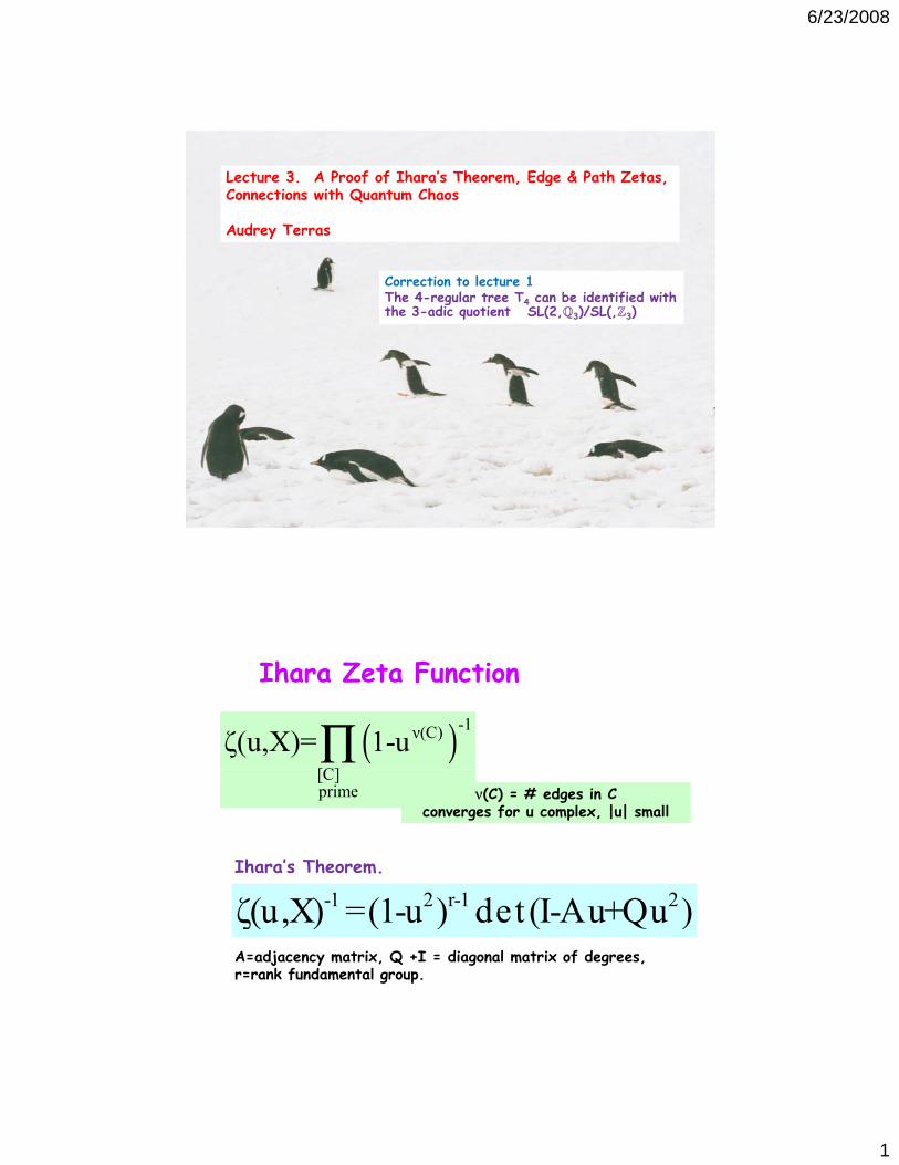
Basic Assumptions

graphs are

connectedconnected,

with r=rank fundamental group > 1,

no degree 1 vertices (called leaf vertex, hair, danglers, ...)

Outline of Talk:1) Bass’s proof of Ihara’s theorem. It involves defining an edge zeta f h bl

g gfunction with more variables coming from pairs of directed edges of the graph

2) Path zeta function which depends only on variables from the edges corresponding to generators of thecorresponding to generators of the fundamental group of the graph

3) a bit of quantum chaos for the W1matrix

6/23/2008

3

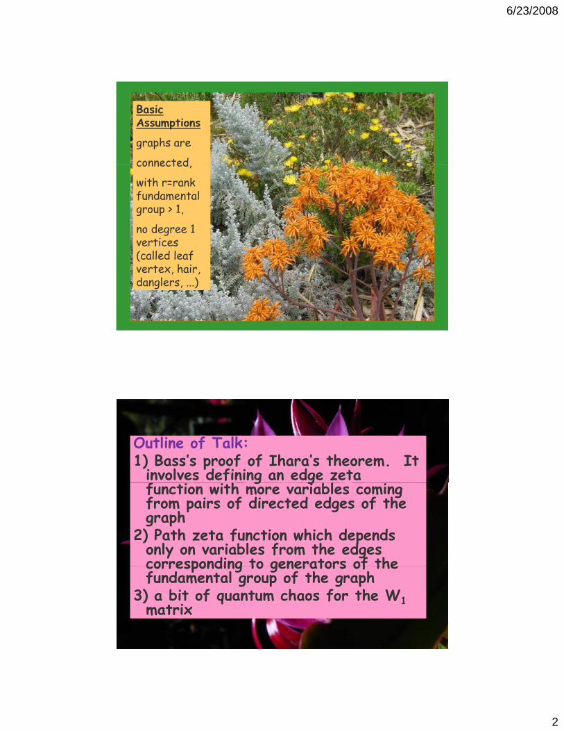
Edge ZetasOrient the edges of the graph. Multiedge matrix W has ab entry wab in C, w(a,b)=wab if the edges a and b look like

a band a is not

a b

1 1 2 2 3 1( ) ( , ) ( , ) ( , ) ( , )EN C w a a w a a w a a w a a=

Otherwise set wab=0.

For a prime C = a1a2…as, define the edge norm

the inverse of b

1 1 2 2 3 1( ) ( , ) ( , ) ( , ) ( , )E s s sN C w a a w a a w a a w a a−

( ) 1

[ ]

( , ) 1 ( )E EC

W X N Cζ −= −∏Define the edge zeta for small |wab| as

Properties of Edge Zeta

Ihara ζ = ζE(W,X)| non-0 w(i,j)=u

edge e deletionζE (W,X-e)=ζE (W,X)|0=w(i,j), if i or j=e

6/23/2008

4

( ) 1( ) d tW X I Wζ −

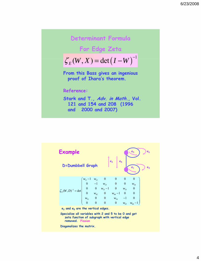
Determinant Formula

For Edge Zeta

( )( , ) detE W X I Wζ = −From this Bass gives an ingenious

proof of Ihara’s theorem.

Reference:Stark and T., Adv. in Math., Vol.

121 and 154 and 208 (1996 and 2000 and 2007)

Example

D=Dumbbell Graphe2 e5

e1 e4

e3 e6

11 12

23 26

33 351

42 44

51 54

1 0 0 0 00 1 0 00 0 1 0 0

( , ) det0 0 1 0 0

0 0 1 00 0 0 0 1

E

w ww w

w wW D

w ww w

ζ −

−⎛ ⎞⎜ ⎟−⎜ ⎟⎜ ⎟−

= ⎜ ⎟−⎜ ⎟⎜ ⎟−⎜ ⎟⎜ ⎟⎝ ⎠65 660 0 0 0 1w w⎜ ⎟−⎝ ⎠

e2 and e5 are the vertical edges.

Specialize all variables with 2 and 5 to be 0 and get zeta function of subgraph with vertical edge removed. Fission

Diagonalizes the matrix.

6/23/2008

5

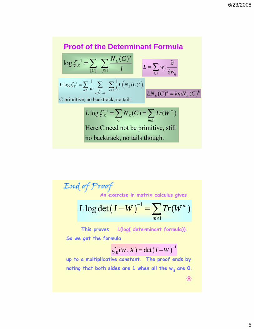
Proof of the Determinant Formula1

[ ] 1

( )logj

EE

C j

N Cj

ζ −

≥

=∑ ∑,

iji j ij

L ww∂=

∂∑,i j ij

( )1

1 1( )

1 1log ( ) ,

C primitive, no backtrack, no tails

kE E

m C kC m

L L N Cm k

ν

ζ −

≥ ≥=

=∑ ∑ ∑( ) ( )k k

E ELN C kmN C=

1l ( ) ( )mL N C T Wζ − ∑ ∑1

1

log ( ) ( )

Here C need not be primitive, still no backtrack, no tails though.

mE E

C m

L N C Tr Wζ≥

= =∑ ∑

( ) 1

1log det ( )mL I W Tr W−

≥

− =∑An exercise in matrix calculus gives

1m≥

This proves L(log( determinant formula)).

So we get the formula

( ) 1( , ) detE W X I Wζ −= −up to a multiplicative constant. The proof ends by

noting that both sides are 1 when all the wij are 0.

6/23/2008

6

( ) 1( , ) detE W X I Wζ −= −

1 2 1 2( , ) (1 ) det( )rV u X u I Au Quζ − −= − − +

1, if v is starting vertex of edge e0, otherwiseves⎧

= ⎨⎩

Define Define starting matrix S and terminal matrix T

| |

| |

00E

E

IJ

I⎛ ⎞

= ⎜ ⎟⎝ ⎠

Part 1 of Bass Proof

0, otherwise⎩1, if v is the terminal vertex of edge e0, otherwisevet ⎧

= ⎨⎩

, TJ=Si t t ( d) f i d ( t t) f

SJ T=Then, recalling our edge numbering system, we see that

j j+|E|since start (end) of e is end (start) of et

|V| T , Q+I t tA S SS TT= = =Note: matrix A counts number of undirected edges connecting 2 distinct vertices and twice # of loops at each vertex. Q+I = diagonal matrix of degrees of vertices

6/23/2008

7

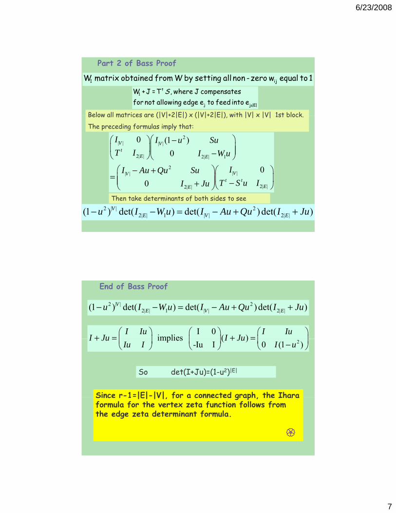
1 ijW matrix obtained from W by setting all non -zero w equal to 1t

1

j j±|E|

W +J =T , where J compensates for not allowing edge e to feed into e

S

Below all matrices are (|V|+2|E|) x (|V|+2|E|) with |V| x |V| 1st block

Part 2 of Bass Proof

2| | | |

2| | 2| | 1

2| || |

0 (1 )0

0

V Vt

E E

VV

I I u SuT I I W u

II Au Qu Su

⎛ ⎞−⎛ ⎞⎜ ⎟⎜ ⎟⎜ ⎟−⎝ ⎠⎝ ⎠

⎛ ⎞− + ⎛ ⎞⎜ ⎟⎜ ⎟

Below all matrices are (|V|+2|E|) x (|V|+2|E|), with |V| x |V| 1st block.

The preceding formulas imply that:

| || |

2| |2| |0VV

t tEE

QT S u II Ju⎛ ⎞

= ⎜ ⎟⎜ ⎟⎜ ⎟ −+ ⎝ ⎠⎝ ⎠Then take determinants of both sides to see

2 | | 22| | 1 | | 2| |(1 ) det( ) det( )det( )V

E V Eu I W u I Au Qu I Ju− − = − + +

2 | | 22| | 1 | | 2| |(1 ) det( ) det( )det( )V

E V Eu I W u I Au Qu I Ju− − = − + +

I 0implies ( )

I Iu I IuI Ju I Ju

⎛ ⎞ ⎛ ⎞ ⎛ ⎞+ = + =⎜ ⎟ ⎜ ⎟ ⎜ ⎟

End of Bass Proof

2 implies ( )-Iu I 0 (1 )

I Ju I JuIu I I u

+ = + =⎜ ⎟ ⎜ ⎟ ⎜ ⎟−⎝ ⎠ ⎝ ⎠ ⎝ ⎠

So det(I+Ju)=(1-u2)|E|

Since r-1=|E|-|V| for a connected graph the IharaSince r 1 |E| |V|, for a connected graph, the Ihara formula for the vertex zeta function follows from the edge zeta determinant formula.

6/23/2008

8

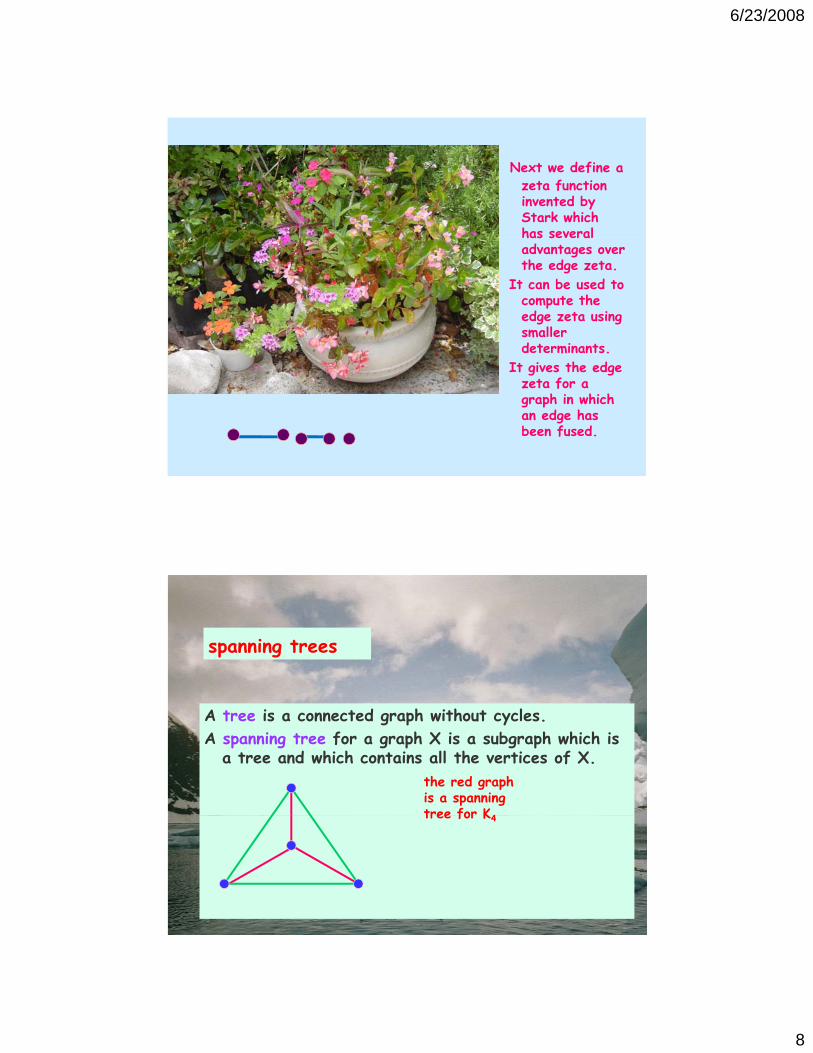
Next we define a zeta function invented by Stark which has severalhas several advantages over the edge zeta.

It can be used to compute the edge zeta using smaller determinants.

It gives the edge zeta for a graph in which an edge has been fused.

spanning trees

A tree is a connected graph without cycles.A spanning tree for a graph X is a subgraph which is

a tree and which contains all the vertices of X.the red graph is a spanning tree for K4tree for K4

6/23/2008

9

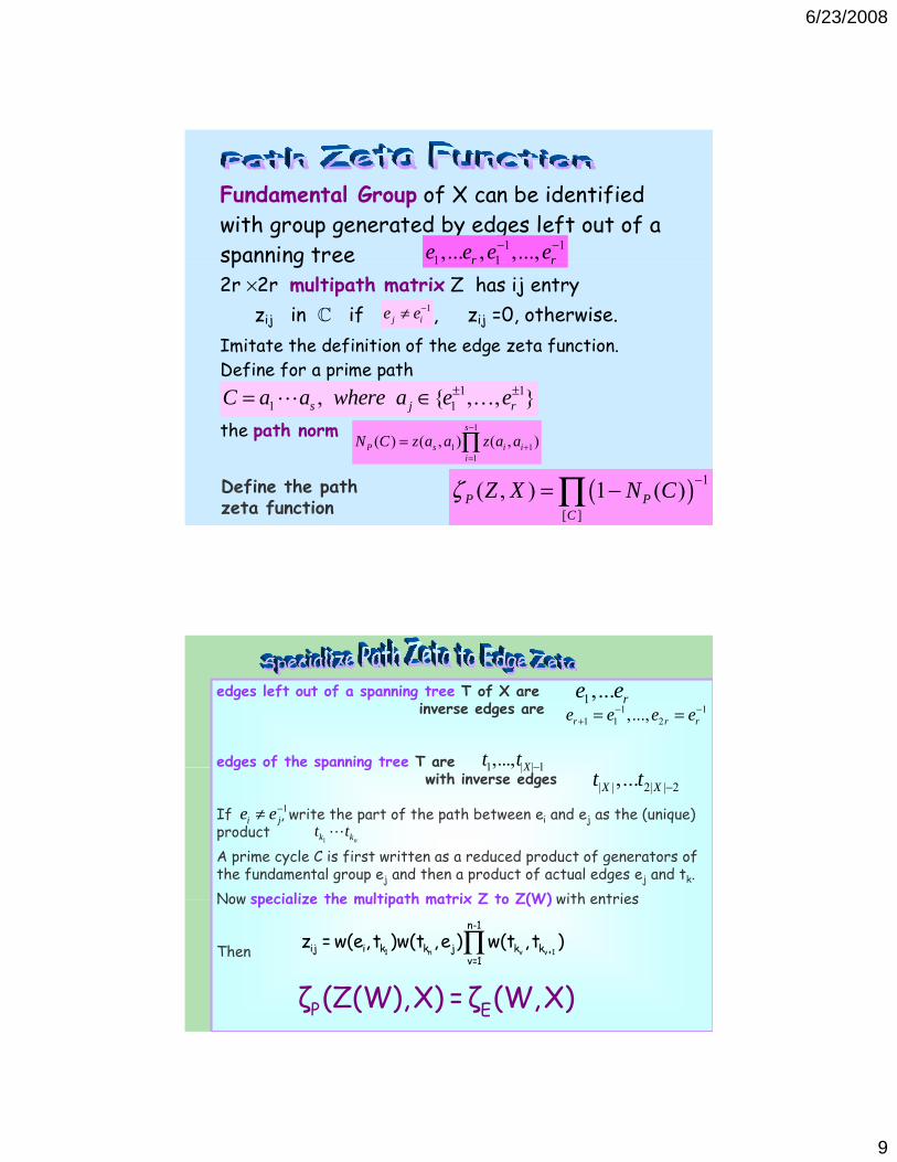
Fundamental Group of X can be identified with group generated by edges left out of a spanning tree 1 1

1 1,... , ,...,r re e e e− −spanning tree

Imitate the definition of the edge zeta function. Define for a prime path

1 1{ }C h ± ±

2r ×2r multipath matrix Z has ij entry zij in C if 1

j ie e−≠ , zij =0, otherwise.

1 1, , , ,r r

1 11 1, { , , }s j rC a a where a e e± ±= ∈ …

the path norm 1

1 11

( ) ( , ) ( , )s

P s i ii

N C z a a z a a−

+=

= ∏

( ) 1

[ ]

( , ) 1 ( )P PC

Z X N Cζ −= −∏Define the path zeta function

edges left out of a spanning tree T of X are inverse edges are

edges of the spanning tree T are

1,... re e1 1

1 1 2,...,r r re e e e− −+ = =

1 | | 1,..., Xt t −g f p gwith inverse edges

If , write the part of the path between ei and ej as the (unique) product A prime cycle C is first written as a reduced product of generators of the fundamental group ej and then a product of actual edges ej and tk.Now specialize the multipath matrix Z to Z(W) with entries

1 | | 1, , X −

| | 2| | 2,...X Xt t −

1i je e−≠

1 nk kt t

Now specialize the multipath matrix Z to Z(W) with entries

Then ∏1 n ν ν+1

n-1

ij i jk k k kν=1

z = w(e ,t )w(t ,e ) w(t ,t )

P Eζ (Z(W),X) =ζ (W,X)

6/23/2008

10

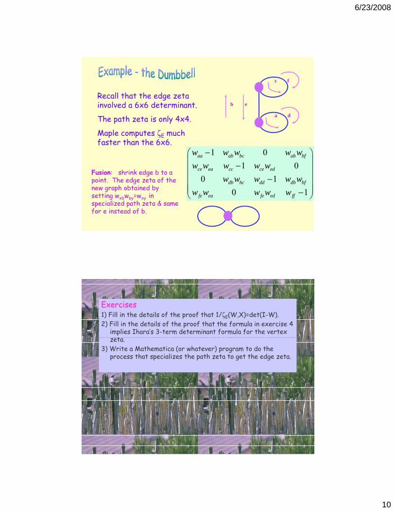
Recall that the edge zeta involved a 6x6 determinant. b e

a d

c f

The path zeta is only 4x4.

Maple computes ζE much faster than the 6x6.

1 01 0

aa ab bc ab bf

ce ea cc ce ed

w w w w ww w w w w

−⎛ ⎞⎜ ⎟−⎜ ⎟⎜ ⎟

a d

Fusion: shrink edge b to a0 1

0 1db bc dd db bf

fe ea fe ed ff

w w w w ww w w w w

⎜ ⎟⎜ ⎟−⎜ ⎟⎜ ⎟−⎝ ⎠

Fusion: shrink edge b to a point. The edge zeta of the new graph obtained by setting wxbwby=wxy in specialized path zeta & same for e instead of b.

ExercisesExercises1) Fill in the details of the proof that 1/ζE(W,X)=det(I-W).2) Fill in the details of the proof that the formula in exercise 4

implies Ihara’s 3-term determinant formula for the vertex tzeta.

3) Write a Mathematica (or whatever) program to do the process that specializes the path zeta to get the edge zeta.

6/23/2008

11

4) Prove that if

( ) 1log det ( )mL I W Tr W−− =∑,

iji j ij

L ww∂=

∂∑

( )1

log det ( )m

L I W Tr W≥

− =∑

Hint: Use the fact that you can write the matrix W (which is not symmetric) as a product W=U-1TU, where U is orthogonal and T is upper triangular by Gram-Schmidt.

A Taste of Random Matrix Theory / Quantum Chaos

a reference with some background on the interest in random matrices in number theory and quantum physics:A.Terras, Arithmetical quantum chaos, IAS/Park City Math. Series, Vol. 12 (2007).

6/23/2008

12

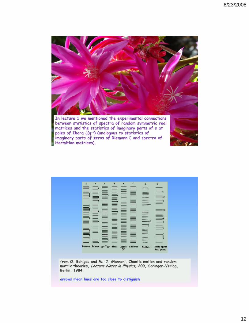
In lecture 1 we mentioned the experimental connections between statistics of spectra of random symmetric real matrices and the statistics of imaginary parts of s at poles of Ihara ζ(q-s) (analogous to statistics of imaginary parts of zeros of Riemann ζ and spectra of Hermitian matrices).

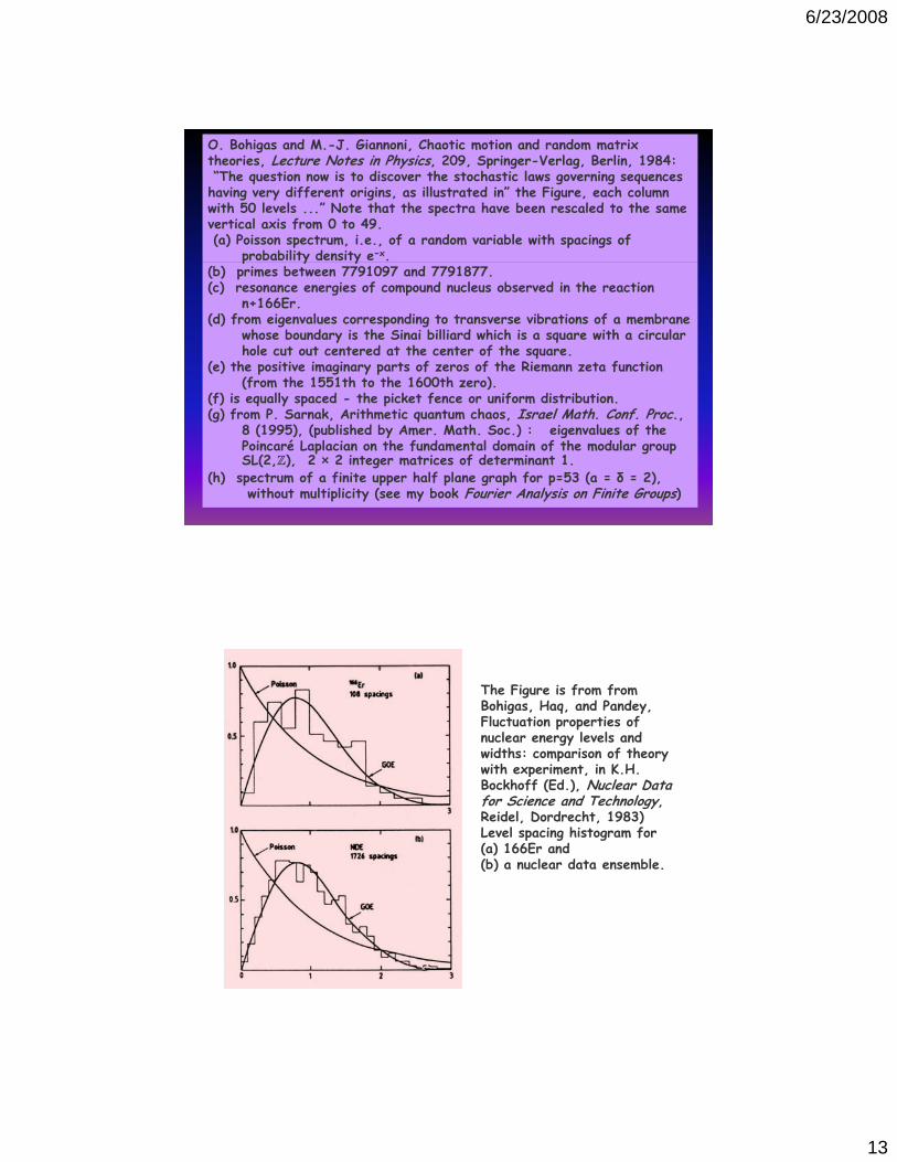
from O. Bohigas and M.-J. Giannoni, Chaotic motion and random matrix theories, Lecture Notes in Physics, 209, Springer-Verlag, Berlin, 1984:

arrows mean lines are too close to distiguish

6/23/2008

13

O. Bohigas and M.-J. Giannoni, Chaotic motion and random matrix theories, Lecture Notes in Physics, 209, Springer-Verlag, Berlin, 1984:“The question now is to discover the stochastic laws governing sequences having very different origins, as illustrated in” the Figure, each column with 50 levels ...” Note that the spectra have been rescaled to the same vertical axis from 0 to 49.(a) Poisson spectrum, i.e., of a random variable with spacings of

probability density e−x. p y y(b) primes between 7791097 and 7791877. (c) resonance energies of compound nucleus observed in the reaction

n+166Er. (d) from eigenvalues corresponding to transverse vibrations of a membrane

whose boundary is the Sinai billiard which is a square with a circular hole cut out centered at the center of the square.

(e) the positive imaginary parts of zeros of the Riemann zeta function(from the 1551th to the 1600th zero).

(f) i ll d th i k t f if di t ib ti(f) is equally spaced - the picket fence or uniform distribution. (g) from P. Sarnak, Arithmetic quantum chaos, Israel Math. Conf. Proc.,

8 (1995), (published by Amer. Math. Soc.) : eigenvalues of the Poincaré Laplacian on the fundamental domain of the modular group SL(2,Z), 2 × 2 integer matrices of determinant 1.

(h) spectrum of a finite upper half plane graph for p=53 (a = δ = 2), without multiplicity (see my book Fourier Analysis on Finite Groups)

The Figure is from fromBohigas, Haq, and Pandey, Fluctuation properties of nuclear energy levels and widths: comparison of theory with experiment in K Hwith experiment, in K.H. Bockhoff (Ed.), Nuclear Data for Science and Technology, Reidel, Dordrecht, 1983) Level spacing histogram for (a) 166Er and (b) a nuclear data ensemble.

6/23/2008

14

Wigner surmise for spacings of spectra of random symmetric real matricesThis means that you arrange the eigenvalues) Ei in decreasing order: E1 ≥ E2 ≥ ・ ・ ・ ≥ En. Assume that the eigenvalues are normalized so that the mean of the level spacings |Ei−Ei 1| is 1so that the mean of the level spacings |Ei Ei+1| is 1.

Wigner’s Surmise from 1957 says the level (eigenvalue) spacing histogram is ≈ the graph of the function ½πxexp(−πx2/4) ,if the mean spacing is 1. In 1960, Gaudin and Mehta found the correct distribution function which is close to Wigner’s. The correct graph is labeled GOE in the Figure preceding. Note the level repulsion indicated by the vanishing of the function at the origin. Also in the preceding Figure, we see the Poisson density which is e−x.p g g , y

A reference is Mehta, Random Matrices.

Now we wish to add a new column to earlier figure - spacings of the eigenvalues of the W1 matrix of a graphCall this exercise 5 or, more accurately perhaps, research project 1.

6/23/2008

15

Here although W1 is not symmetric, the nearest neighbor spacing (i.e., histogram of minimum distances between eigenvalues) is also of interest.

many references on the study of spacings of spectra of non-Hermitian or non-symmetric matrices. I did find one: P. LeBoef, Random matrices random polynomials and Coulomb systemsRandom matrices, random polynomials, and Coulomb systems. He studies the ensemble of matrices introduced by J. Ginibre, J. Math. Phys. 6, 440 (1965).An approximation to the distribution of spacings of eigenvalues of a complex matrix (analogous to the Wigner surmise for Hermitian matrices) is: 4

44 53 454

4

ss e

⎛ ⎞−Γ⎜ ⎟⎝ ⎠⎛ ⎞Γ⎜ ⎟

⎝ ⎠

Since our matrix is real, this will probably not be the correct Wigner surmise.I haven’t done this experiment yet. In what follows, I just plot the reciprocals of the eigenvalues of W1 - the poles of Ihara zeta for various graphs. The distribution looks rather different than that of a random real matrix with the properties of W1.

Statistics of the poles of Ihara zeta or reciprocals of eigenvalues of the Edge Matrix W1

Define W1 to be the 0,1 matrix you get from W by setting all non-0 entries of W to be 1.

Theorem. ζ(u,X)-1=det(I-W1u).

Corollary. The poles of Ihara zeta are the reciprocals of the eigenvalues of W1.

The pole R of zeta is:The pole R of zeta is:

R=1/Perron-Frobenius eigenvalue of W1.

6/23/2008

16

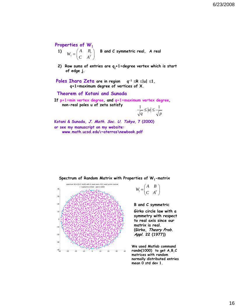
Properties of W1

2) Row sums of entries are qj+1=degree vertex which is start f d

1 T

A BW

C A⎛ ⎞= ⎜ ⎟⎝ ⎠

1) , B and C symmetric real, A real

of edge j.

Poles Ihara Zeta are in region q-1 ≤R ≤|u| ≤1, q+1=maximum degree of vertices of X.

Theorem of Kotani and SunadaIf p+1=min vertex degree, and q+1=maximum vertex degree,

n n l p l f t ti fnon-real poles u of zeta satisfy

Kotani & Sunada, J. Math. Soc. U. Tokyo, 7 (2000) or see my manuscript on my website:

www.math.ucsd.edu\~aterras\newbook.pdf

1 1uq p

≤ ≤

30

40

spectrum W=A B;C trn(A) with A rand norm, B,C rand symm normalr =sqrt(n)*(1+2.5)/2 and n=1000

Spectrum of Random Matrix with Properties of W1-matrix

1 T

A BW

C A⎛ ⎞= ⎜ ⎟⎝ ⎠

-20

-10

0

10

20 B and C symmetricGirko circle law with a symmetry with respect to real axis since our matrix is real. (Girko, Theory Prob. Appl. 22 (1977))

-40 -30 -20 -10 0 10 20 30 40-40

-30

We used Matlab command randn(1000) to get A,B,Cmatrices with random normally distributed entries mean 0 std dev 1.

6/23/2008

17

What is the meaning of the RH

for irregular graphs?

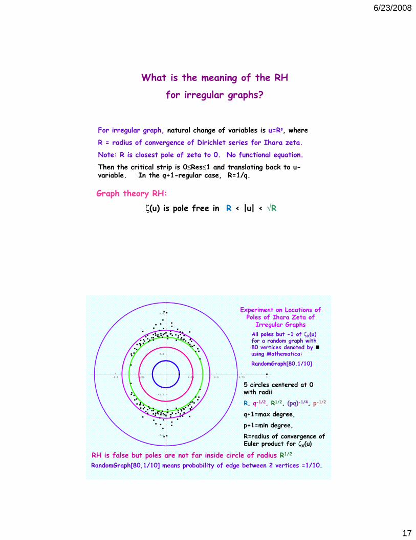
For irregular graph, natural change of variables is u=Rs, where

R = radius of convergence of Dirichlet series for Ihara zeta.

Note: R is closest pole of zeta to 0. No functional equation.

Then the critical strip is 0≤Res≤1 and translating back to u-variable. In the q+1-regular case, R=1/q.

Graph theory RH:

ζ(u) is pole free in R < |u| < √R

0.2

0.4

0.6Experiment on Locations of

Poles of Ihara Zeta of Irregular Graphs

All poles but -1 of ζX(u) for a random graph with 80 vertices denoted by using Mathematica:

-0.5 -0.25 0.25 0.5 0.75 1

-0.4

-0.2

5 circles centered at 0 with radii

R, q-1/2, R1/2, (pq)-1/4, p-1/2

q+1=max degree,

g

RandomGraph[80,1/10]

-0.6

p+1=min degree,

R=radius of convergence of Euler product for ζX(u)

RH is false but poles are not far inside circle of radius R1/2

RandomGraph[80,1/10] means probability of edge between 2 vertices =1/10.

6/23/2008

18

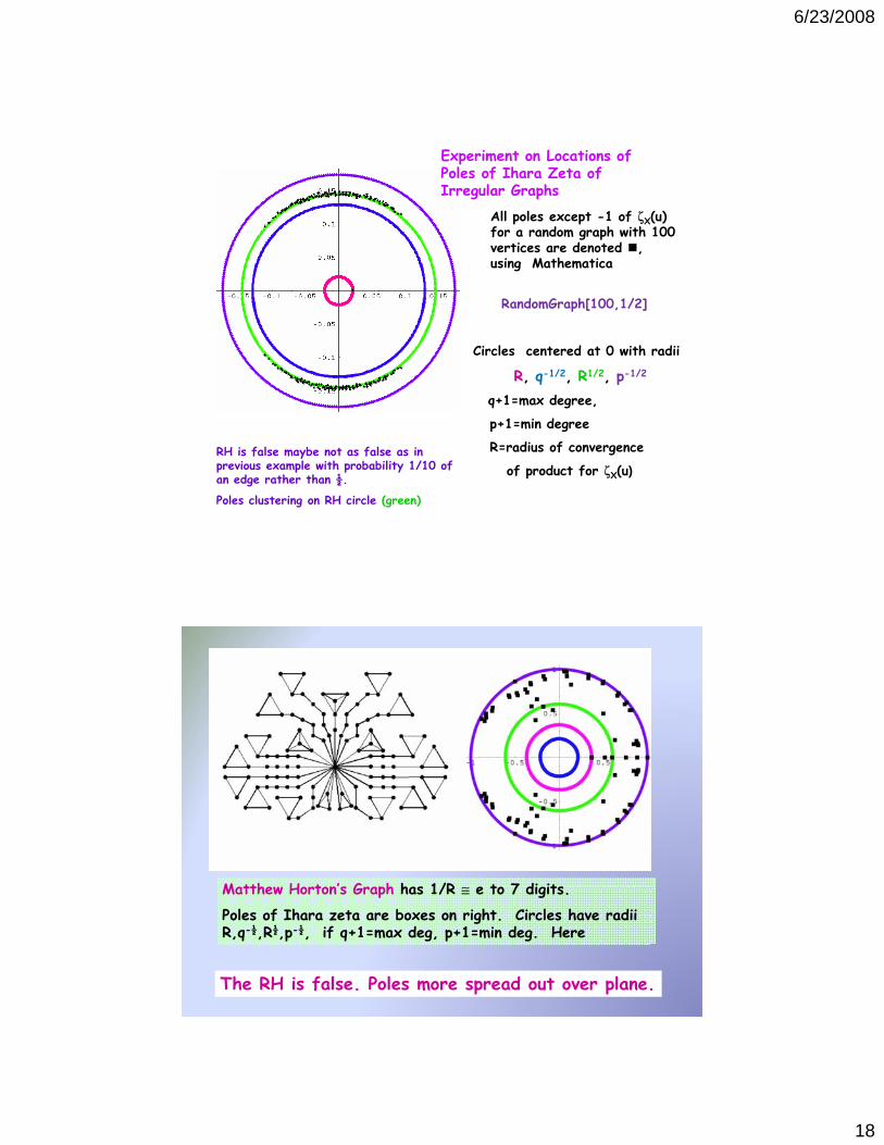
Experiment on Locations of Poles of Ihara Zeta of Irregular Graphs

All poles except -1 of ζX(u) for a random graph with 100 vertices are denoted ,

M husing Mathematica

Circles centered at 0 with radii

R, q-1/2, R1/2, p-1/2

RandomGraph[100,1/2]

q+1=max degree,

p+1=min degree

R=radius of convergence

of product for ζX(u) RH is false maybe not as false as in previous example with probability 1/10 of an edge rather than ½.

Poles clustering on RH circle (green)

M tth H t n’ G ph h 1/R t 7 di itMatthew Horton s Graph has 1/R ≅ e to 7 digits.

Poles of Ihara zeta are boxes on right. Circles have radii R,q-½,R½,p-½, if q+1=max deg, p+1=min deg. Here

The RH is false. Poles more spread out over plane.

6/23/2008

19

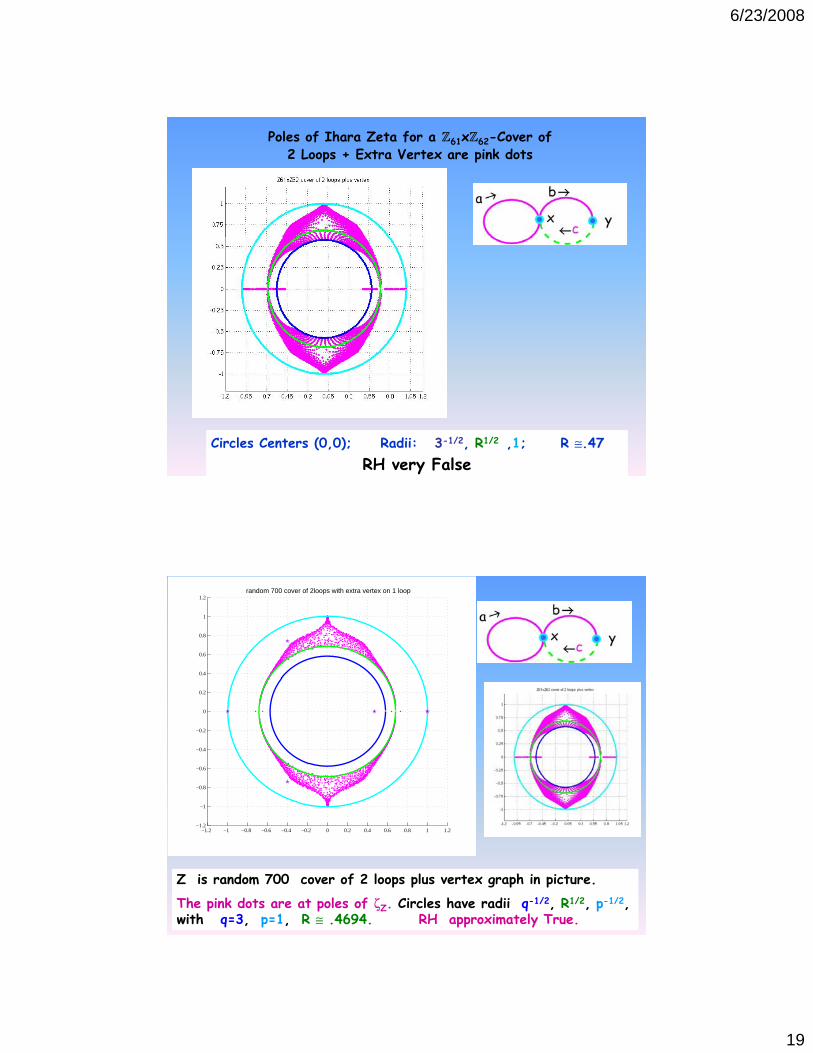
Poles of Ihara Zeta for a Z61xZ62-Cover of 2 Loops + Extra Vertex are pink dots

Circles Centers (0,0); Radii: 3-1/2, R1/2 ,1; R ≅.47RH very False

0.2

0.4

0.6

0.8

1

1.2random 700 cover of 2loops with extra vertex on 1 loop

−1

−0.8

−0.6

−0.4

−0.2

0

0.2

Z is random 700 cover of 2 loops plus vertex graph in picture.

The pink dots are at poles of ζZ. Circles have radii q-1/2, R1/2, p-1/2, with q=3, p=1, R ≅ .4694. RH approximately True.

−1.2 −1 −0.8 −0.6 −0.4 −0.2 0 0.2 0.4 0.6 0.8 1 1.2−1.2

6/23/2008

20

References: 3 papers with Harold Stark in Advances in Math.Paper with Matthew Horton & Harold Stark in Snowbird Proceedings, Contemporary Mathematics, Volume 415 (2006)

See my draft of a book:

Quantum Graphs and Their Applications, Contemporary Mathematics, v. 415, AMS, Providence, RI 2006.

See my draft of a book:

www.math.ucsd.edu/~aterras/newbook.pdf

Draft of new paper joint with Horton & Stark: also on my website

www.math.ucsd.edu/~aterras/cambridge.pdf

There was a graph zetas special session of this AMS meeting –many interesting papers some on my website.

For work on directed graphs, see Matthew Horton, Ihara zeta functions of digraphs, Linear Algebra and its Applications, 425 (2007) 130–142.

work of Angel, Friedman and Hoory giving analog of Alon conjecture for irregular graphs, implying our Riemann Hypothesis (see Joel Friedman’s website: www.math.ubc.ca/~jf)

The End