Electrodynamics - A Summary

1 Preliminaries

Vector relations:

∇ · ∇ × v = 0 (1.1)∇×∇× v = ∇(∇ · v)−∇2v (1.2)

Divergence & Stokes Theorem: ∫v · dS =

∫∇ · vdV (1.3)∮

v · d` =∫∇× v · dS (1.4)

Delta-function; think about it as filtering out a single value of a function. Use them in representingpoint-charges:

f(x) =∫ ∞−∞

f(x′)δ(x− x′)dx′ (1.5)

Operators: If the following are used to operate on a plane wave, then we find the following results:

∂

∂t→ −iω ∇× → ik× (1.6)

Maxwells equations:

∇ ·E =ρ

ε0(1.7)

∇ ·B = 0 (1.8)

∇×E = −∂B∂t

(1.9)

∇×B = µ0J + µ0ε0∂E

∂t(1.10)

We have the relation:

B =1ck̂ ×E (1.11)

In linear media:

D = εrε0E H =1

µrµ0B (1.12)

In vacuum, Maxwells equations may be written:

∇×H = J +∂D

∂t∇ ·D = ρ (1.13)

The Lorentz force law, and Poynting vector:

F = q(E + v ×B) P = E ×H (1.14)

1

2 Fields 1

A useful way to think about all of these integrals: The distribution is always in the primed coor-dinate system. The integrals sweep over the distribution, picking out the little bits of charge, thenseamlessly adds them together via the integral.

If the observation point is some r, then if there is a point charge, at r′, the electric field at theobservation point is given by:

E(r) =q

4πε0r − r′

|r − r′|3(2.1)

The electric (scalar) potential, due to some continuous distribution of charge, residing at primedcoordinates, is given by:

φ(r) =q

4πε0

∫ρ(r′)|r − r′|

d3r′ (2.2)

The electric field is given by (static fields only):

E = −∇φ (2.3)

We easily combine this and Gauss’ law, to derive:

∇2φ = − ρ

ε0(2.4)

We have, by analogy, this magnetic vector potential:

A(r) =µ0

4π

∫J(r′)|r − r′|

d3r′ (2.5)

The magnetic field is related to the vector potential via:

B = ∇×A (2.6)

We use this, and the Coulomb gauge (for static fields), ∇ ·A = 0, to derive:

∇2A = −µ0J (2.7)

The continuity equation, for charges & currents:

∇ · J +∂ρ

∂t= 0 (2.8)

3 Fields in Materials

If we have an interface, region 1 into region 2. At the interface, is some charge distribution σ. Then:

D2,⊥ −D1,⊥ = σ (3.1)

So, we also have the following relations:

εr,2ε0E2,⊥ − εr,1ε0E1,⊥ = σ (3.2)

εr,2ε0∂V2

∂r− εr,1ε0

∂V1

∂r= −σ (3.3)

2

4 Gauges

The Coulomb gauge, used for static fields:

∇ ·A = 0 (4.1)

The Lorentz gauge, used for time-varying fields:

∇ ·A+1c2∂2φ

∂t2= 0 (4.2)

We then have that fields can be found from potentials via:

E = −∇φ− ∂A

∂tB = ∇×A (4.3)

The choices of φ,A are arbitrary, up to certain factors:

φ′ = φ− ∂χ

∂tA′ = A+∇χ (4.4)

Under the Lorentz gauge, we are able to derive the following wave-equation:(∇2 − 1

c2∂2

∂t2

)A = −µ0J (4.5)

To do this, put E into Gauss’ law, and put both E,B into Amperes law. This will produce twocoupled wave equations. To un-couple, use the Lorentz gauge. We end up with:

�2φ = − ρ

ε0�2A = −µ0J �2 ≡ 1

c2∂2

∂t2−∇2 (4.6)

5 Energy in Fields

The energy density in each field is given by:

UE = ε0

∫|E|2d3r (5.1)

UB = µ0

∫|B|2d3r (5.2)

The Poynting vector is the energy flow per unit area, per unit time:

P = E ×H (5.3)

These above equations can then be bought together into Poyntings theorem, which gives the rateof flow of energy:

dW

dt= − ∂

∂t(UE + UM )−

∫P · dS (5.4)

We will often denote the Poynting vector in terms of the total flux of energy, per unit time:

P̄ =∫P · dS

3

6 Laplace’s Equation

The solution to Laplaces equation ∇2φ = 0, in cylindrical polars, are Bessel functions. In Sphericalpolars, the solution has the form:

V (r, θ, ϕ) =∑`m

(A`mr

` +B`m

r`+1

)Y`m(θ, ϕ)

If the system has axial symmetry, then this reduces to (and this is more commonly used):

V (r, θ) ==∑`m

(A`r

` +B`

r`+1

)P`(cos θ) (6.1)

If there is total angular symmetry to the system, then the solution is of the form:

V (r) = A+B

r

7 Multipole Expansions

We have:

V (r) =1

4πε0

∑`

1r`+1

∫r′`P`(cos γ)ρ(r′)d3r′ (7.1)

With monopole and dipole moments being:

q ≡∫ρ(r′)d3r′ p =

∫r′ cos γρ(r′)d3r′ (7.2)

Where γ ≡ θ′ − θ. It is also usual to take the vector version of the dipole moment to be:

p =∫r′ρ(r′)d3r′

So that the potential due to a dipole is:

V (r) =1

4πε0r2p · r̂ (7.3)

The magnetic dipole moment, which is derived in a very similar way, is:

m =12

∫r′ × J(r′)d3r′ (7.4)

With the magnetic potential due to a magnetic dipole being given by:

A(r) =µ0

4πm× rr3

4

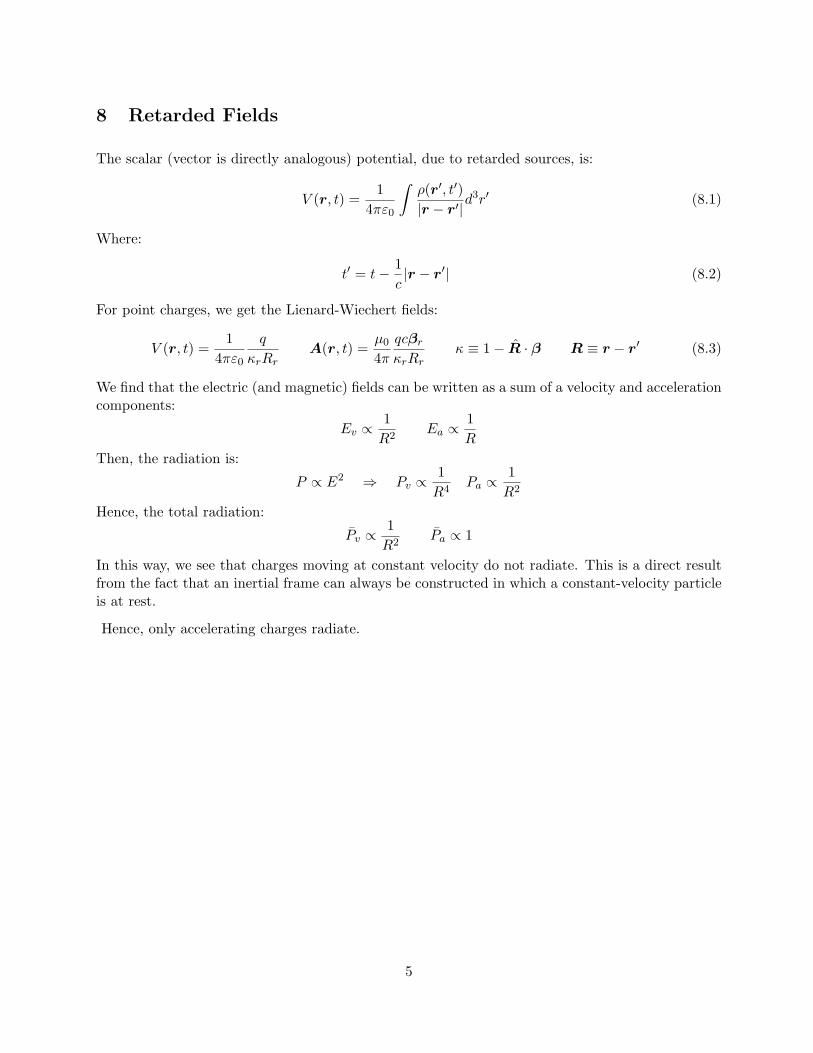
8 Retarded Fields

The scalar (vector is directly analogous) potential, due to retarded sources, is:

V (r, t) =1

4πε0

∫ρ(r′, t′)|r − r′|

d3r′ (8.1)

Where:

t′ = t− 1c|r − r′| (8.2)

For point charges, we get the Lienard-Wiechert fields:

V (r, t) =1

4πε0q

κrRrA(r, t) =

µ0

4πqcβr

κrRrκ ≡ 1− R̂ · β R ≡ r − r′ (8.3)

We find that the electric (and magnetic) fields can be written as a sum of a velocity and accelerationcomponents:

Ev ∝1R2

Ea ∝1R

Then, the radiation is:

P ∝ E2 ⇒ Pv ∝1R4

Pa ∝1R2

Hence, the total radiation:

P̄v ∝1R2

P̄a ∝ 1

In this way, we see that charges moving at constant velocity do not radiate. This is a direct resultfrom the fact that an inertial frame can always be constructed in which a constant-velocity particleis at rest.

Hence, only accelerating charges radiate.

5