Microscopic electrodynamics - Virginia Tech€¦ · Continuity equation r B 1 c2 @ tE = 0j r(r ......

Microscopic electrodynamics

Trond Saue (LCPQ, Toulouse) Microscopic electrodynamics Virginia Tech 2015 1 / 46

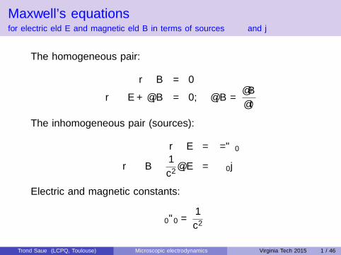
Maxwell’s equationsfor electric field E and magnetic field B in terms of sources ρ and j

The homogeneous pair:

∇ · B = 0

∇× E + ∂tB = 0; ∂tB =∂B

∂t

The inhomogeneous pair (sources):

∇ · E = ρ/ε0

∇× B− 1

c2∂tE = µ0j

Electric and magnetic constants:

µ0ε0 =1

c2


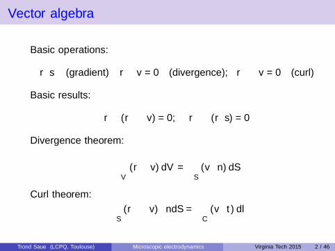
Vector algebra

Basic operations:

∇s (gradient) ∇ · v = 0 (divergence); ∇× v = 0 (curl)

Basic results:

∇ · (∇× v) = 0; ∇× (∇s) = 0

Divergence theorem:

ˆV

(∇ · v) dV =

ˆS

(v · n) dS

Curl theorem: ˆS

(∇× v) · ndS =

˛C

(v · t) dl


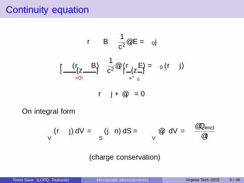
Continuity equation

∇× B− 1

c2∂tE = µ0j

∇ · (∇× B)︸︷︷︸=0!

− 1

c2∂t (∇ · E)︸︷︷︸

ρ/ε0

= µ0 (∇ · j)

∇ · j + ∂tρ = 0

On integral form

ˆV

(∇ · j) dV =

ˆS

(j · n) dS = −ˆ

V∂tρdV = −∂Qencl

∂t

(charge conservation)


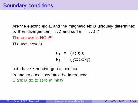
Boundary conditions

Are the electric field E and the magnetic field B uniquely determinedby their divergence (∇ · . . .) and curl (∇× . . .) ?

The answer is NO !!!!

The two vectors

F1 = (0, 0, 0)

F2 = (yz , zx , xy)

both have zero divergence and curl.

Boundary conditions must be introduced:E and B go to zero at infinity


Maxwell’s equations: solutions


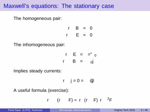
Maxwell’s equations: The stationary case

The homogeneous pair:

∇ · B = 0

∇× E = 0

The inhomogeneous pair:

∇ · E = ρ/ε0

∇× B = µ0j

Implies steady currents:

∇ · j = 0 = −∂tρ

A useful formula (exercise):

∇× (∇× F) =∇ (∇ · F)−∇2F


Maxwell’s equations: The stationary caseElectrostatics

∇2E =∇× (∇× E)︸︷︷︸=0

−∇ (∇ · E)︸︷︷︸ρ/ε0

= −∇ρ/ε0

Simeon Denis Poisson

(1781-1840)

Each component of the electric fieldfulfills the Poisson equation:

∇2Ψ (r1, t) = f (r1, t)

with solutions

Ψ (r1, t) = − 1

4π

ˆf (r2, t)

r12d3r2


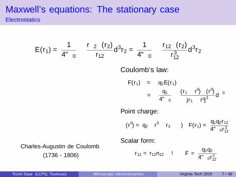
Maxwell’s equations: The stationary caseElectrostatics

E (r1) =1

4πε0

ˆ ∇2ρ (r2)

r12d3r2 =

1

4πε0

ˆr12ρ (r2)

r312d3r2

Charles-Augustin de Coulomb

(1736 - 1806)

Coulomb’s law:

F(r1) = q1E(r1)

=q1

4πε0

ˆ(r1 − r′) ρ (r′)

|r1 − r′|3dτ ′

Point charge:

ρ(r′) = q2δ(r′ − r2

)⇒ F(r1) =

q1q2r124πε0r 312

Scalar form:

r12 = r12n12 → F =q1q2

4πε0r 212


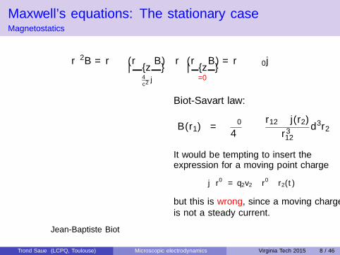
Maxwell’s equations: The stationary caseMagnetostatics

∇2B =∇× (∇× B)︸︷︷︸4πc2

j

−∇ (∇ · B)︸︷︷︸=0

=∇× µ0j

Jean-Baptiste Biot

(1774-1862)

Biot-Savart law:

B(r1) = −µ04π

ˆr12 × j(r2)

r312d3r2

It would be tempting to insert theexpression for a moving point charge

j(r′)

= q2v2δ(r′ − r2(t)

)but this is wrong, since a moving chargeis not a steady current.


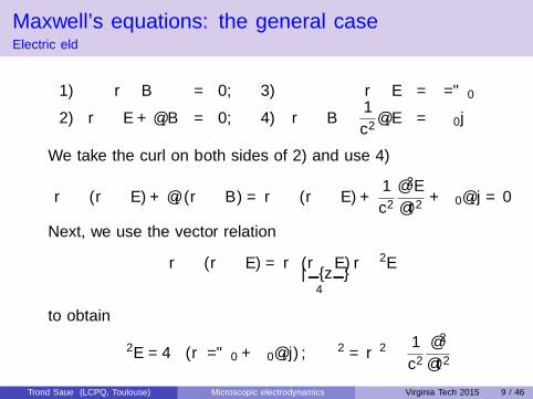
Maxwell’s equations: the general caseElectric field

1) ∇ · B = 0; 3) ∇ · E = ρ/ε0

2) ∇× E + ∂tB = 0; 4) ∇× B− 1

c2∂tE = µ0j

We take the curl on both sides of 2) and use 4)

∇× (∇× E) + ∂t (∇× B) =∇× (∇× E) +1

c2∂2E

∂t2+ µ0∂t j = 0

Next, we use the vector relation

∇× (∇× E) =∇ (∇ · E)︸︷︷︸4πρ

−∇2E

to obtain

�2E = 4π (∇ρ/ε0 + µ0∂t j) ; �2 = ∇2 − 1

c2∂2

∂t2


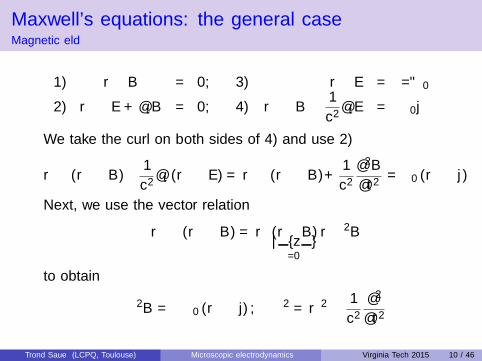
Maxwell’s equations: the general caseMagnetic field

1) ∇ · B = 0; 3) ∇ · E = ρ/ε0

2) ∇× E + ∂tB = 0; 4) ∇× B− 1

c2∂tE = µ0j

We take the curl on both sides of 4) and use 2)

∇× (∇× B)− 1

c2∂t (∇× E) =∇× (∇× B)+

1

c2∂2B

∂t2= µ0 (∇× j)

Next, we use the vector relation

∇× (∇× B) =∇ (∇ · B)︸︷︷︸=0

−∇2B

to obtain

�2B = −µ0 (∇× j) ; �2 = ∇2 − 1

c2∂2

∂t2


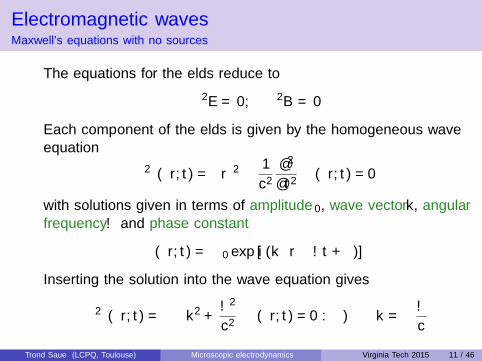
Electromagnetic wavesMaxwell’s equations with no sources

The equations for the fields reduce to

�2E = 0; �2B = 0

Each component of the fields is given by the homogeneous waveequation

�2Ψ (r, t) =

[∇2 − 1

c2∂2

∂t2

]Ψ (r, t) = 0

with solutions given in terms of amplitude Ψ0, wave vector k, angularfrequency ω and phase constant δ

Ψ (r, t) = Ψ0 exp [i (k · r − ωt + δ)]

Inserting the solution into the wave equation gives

�2Ψ (r, t) =

(−k2 +

ω2

c2

)Ψ (r, t) = 0 : ⇒ k = ±ω

c


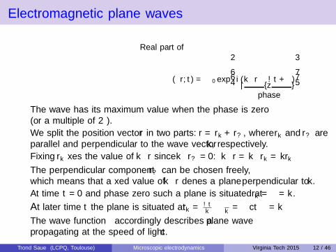
Electromagnetic plane waves

Real part of

Ψ (r, t) = Ψ0 exp

i (k · r − ωt + δ)︸︷︷︸phase

The wave has its maximum value when the phase is zero(or a multiple of 2π).

We split the position vector r in two parts: r = r‖ + r⊥, where r‖ and r⊥ areparallel and perpendicular to the wave vector k, respectively.

Fixing r‖ fixes the value of k · r since k · r⊥ = 0: k · r = k · r‖ = kr‖

The perpendicular component r⊥ can be chosen freely,which means that a fixed value of k · r defines a plane perpendicular to k.

At time t = 0 and phase zero such a plane is situated at r‖ = −δ/k.

At later time t the plane is situated at r‖ = ωtk −

δk = ±ct − δ/k

The wave function Ψ accordingly describes a plane wavepropagating at the speed of light c.


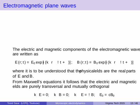
Electromagnetic plane waves

The electric and magnetic components of the electromagnetic waveare written as

E (r, t) = E0 exp [i (k · r − ωt + δ)] ; B (r, t) = B0 exp [i (k · r − ωt + δ)]

where it is to be understood that the physical fields are the real partsof E and B.

From Maxwell’s equations it follows that the electric and magneticfields are purely transversal and mutually orthogonal

k · E = 0; k · B = 0; k× E = ωB; E0 = cB0


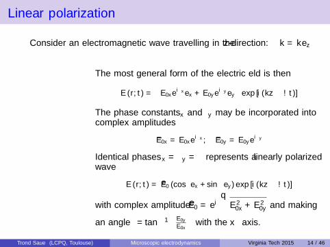
Linear polarization

Consider an electromagnetic wave travelling in the z-direction: k = kez

The most general form of the electric field is then

E (r, t) =(E0xe

iδx ex + E0yeiδy ey

)exp [i (kz − ωt)]

The phase constants δx and δy may be incorporated intocomplex amplitudes

E0x = E0xeiδx ; E0y = E0ye

iδy

Identical phases δx = δy = δ represents a linearly polarizedwave

E (r, t) = E0 (cos θex + sin θey ) exp [i (kz − ωt)]

with complex amplitude E0 = e iδ√E 20x + E 2

0y and making

an angle θ = tan−1(

E0y

E0x

)with the x−axis.


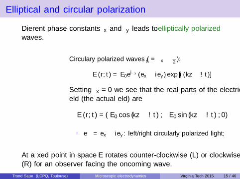
Elliptical and circular polarization

Different phase constants δx and δy leads to elliptically polarizedwaves.

Circulary polarized waves (δy = δx ± π2 ):

E (r, t) = E0eiδx (ex ± iey ) exp [i (kz − ωt)]

Setting δx = 0 we see that the real parts of the electricfield (the actual field) are

E (r, t) = (E0 cos (kz − ωt) ,∓E0 sin (kz − ωt) , 0)

I e± = ex ± iey : left/right circularly polarized light;

At a fixed point in space E rotates counter-clockwise (L) or clockwise(R) for an observer facing the oncoming wave.


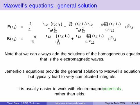
Maxwell’s equations: general solution

E(r1) =1

4π

ˆ {r12ρ (r2, tr )

ε0r312+∂tρ (r2, tr ) r12

ε0r212− µ0∂t j (r2, tr )

c2r12

}d3r2

B(r1) = −µ04π

ˆ {r12 × j (r2, tr )

r312+

r12 × ∂t j (r2, tr )

cr²12

}d3r2

Note that we can always add the solutions of the homogeneous equations,that is the electromagnetic waves.

Jefimenko’s equations provide the general solution to Maxwell’s equations,but typically lead to very complicated integrals.

It is usually easier to work with electromagnetic potentials,rather than fields.


Electromagnetic potentials


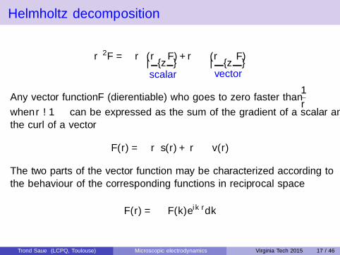
Helmholtz decomposition

∇2F = −∇ (∇ · F)︸︷︷︸scalar

+∇× (∇× F)︸︷︷︸vector

Any vector function F (differentiable) who goes to zero faster than1

rwhen r →∞ can be expressed as the sum of the gradient of a scalar andthe curl of a vector

F(r) = −∇s(r) +∇× v(r)

The two parts of the vector function may be characterized according tothe behaviour of the corresponding functions in reciprocal space

F(r) =

ˆF(k)e ik·rdk


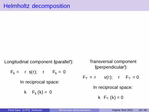
Helmholtz decomposition

Longitudinal component (“parallel”):

F‖ = −∇s(r); ∇× F‖ = 0

In reciprocal space:

k× F‖ (k) = 0

Transversal component(“perpendicular”):

F⊥ =∇× v(r); ∇ · F⊥ = 0

In reciprocal space:

k · F⊥ (k) = 0


PotentialsMaxwell’s equations: homogeneous pair

∇ · B = 0 implies

B = B⊥ =∇× A(r) and B‖ = 0

∇× E +∂B

∂t= 0 then becomes ∇× (E + ∂tA) = 0

and one may writeE + ∂tA = −∇φ(r)

I Longitudinal component: E‖ = −∇φ− ∂tA‖I Transversal component: E⊥ = −∂tA⊥

With the introduction of the scalar potential φ and the vectorpotential A, the homogeneous pair of Maxwell’s equations isautomatically satisfied.


PotentialsMaxwell’s equations: inhomogeneous pair

∇× B− 1

c2∂tE = µ0j becomes

[∇2 − 1

c2∂2

∂t2

]A−∇

[(∇ · A) +

1

c2∂φ

∂t

]= −µ0j

∇ · E = ρ/ε0 becomes

∇2φ+ ∂t (∇ · A) = −ρ/ε0

or [∇2 − 1

c2∂2

∂t2

]φ+ ∂t

[(∇ · A) +

1

c2∂φ

∂t

]= −ρ/ε0


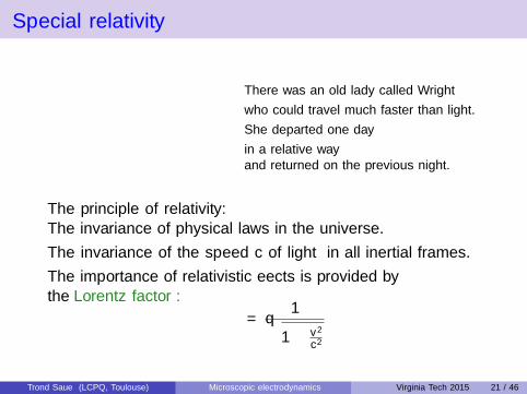
Special relativity

There was an old lady called Wright

who could travel much faster than light.

She departed one day

in a relative wayand returned on the previous night.

The principle of relativity:The invariance of physical laws in the universe.

The invariance of the speed c of light in all inertial frames.

The importance of relativistic effects is provided bythe Lorentz factor:

γ =1√

1− v2

c2


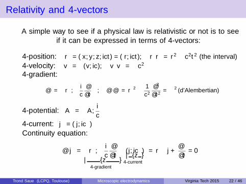
Relativity and 4-vectors

A simple way to see if a physical law is relativistic or not is to seeif it can be expressed in terms of 4-vectors:

4-position: rµ = (x , y , z , ict) = (r, ict); rµrµ = r2 − c2t2 (the interval)

4-velocity: vµ = γ(v, ic); vµvµ = −c24-gradient:

∂µ =

(∇,− i

c

∂

∂t

); ∂µ∂µ = ∇2 − 1

c2∂2

∂t2= �2 (d’Alembertian)

4-potential: Aµ =

(A,

i

cφ

)4-current: jµ = (j, icρ)

Continuity equation:

∂µjµ =

(∇,− i

c

∂

∂t

)︸︷︷︸

4-gradient

(j, icρ)︸︷︷︸4-current

=∇ · j +∂ρ

∂t= 0


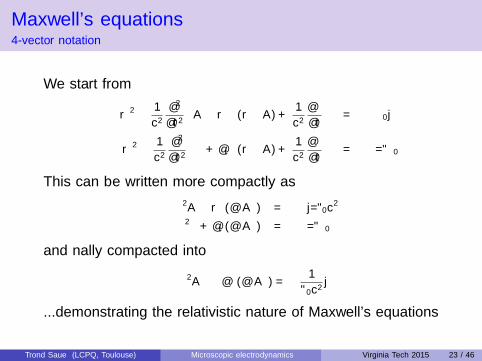
Maxwell’s equations4-vector notation

We start from[∇2 − 1

c2∂2

∂t2

]A−∇

[(∇ · A) +

1

c2∂φ

∂t

]= −µ0j[

∇2 − 1

c2∂2

∂t2

]φ+ ∂t

[(∇ · A) +

1

c2∂φ

∂t

]= −ρ/ε0

This can be written more compactly as

�2A−∇ (∂νAν) = −j/ε0c2

�2φ+ ∂t (∂νAν) = −ρ/ε0

and finally compacted into

�2Aµ − ∂µ (∂νAν) = − 1

ε0c2jµ

...demonstrating the relativistic nature of Maxwell’s equations


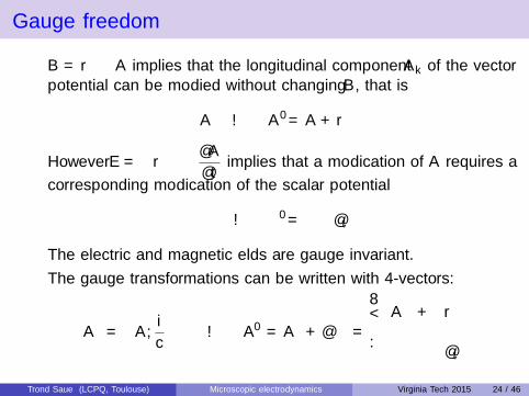
Gauge freedom

B =∇× A implies that the longitudinal component A‖ of the vectorpotential can be modified without changing B, that is

A → A′ = A +∇χ

However E = −∇φ− ∂A

∂timplies that a modification of A requires a

corresponding modification of the scalar potential

φ → φ′ = φ− ∂tχ

The electric and magnetic fields are gauge invariant.

The gauge transformations can be written with 4-vectors:

Aµ =

(A,

i

cφ

)→ A′µ = Aµ + ∂µχ =

A + ∇χ

φ − ∂tχ


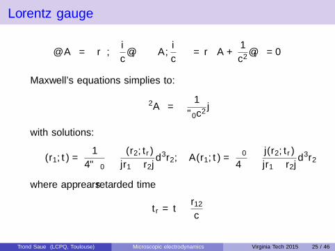
Lorentz gauge

∂αAα =

(∇,− i

c∂t

)·(

A,i

cφ

)=∇·A +

1

c2∂tφ = 0

Maxwell’s equations simplifies to:

�2Aµ = − 1

ε0c2jµ

with solutions:

φ(r1, t) =1

4πε0

ˆρ(r2, tr )

|r1 − r2|d3r2; A(r1, t) =

µ04π

ˆj(r2, tr )

|r1 − r2|d3r2

where apprears retarded time

tr = t − r12c


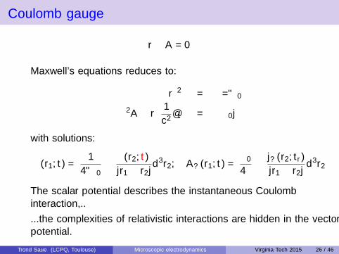
Coulomb gauge

∇ · A = 0

Maxwell’s equations reduces to:

∇2φ = −ρ/ε0

�2A−∇ 1

c2∂tφ = −µ0j

with solutions:

φ(r1, t) =1

4πε0

ˆρ(r2, t)

|r1 − r2|d3r2; A⊥(r1, t) =

µ04π

ˆj⊥(r2, tr )

|r1 − r2|d3r2

The scalar potential describes the instantaneous Coulombinteraction,..

...the complexities of relativistic interactions are hidden in the vectorpotential.


Particles and fields


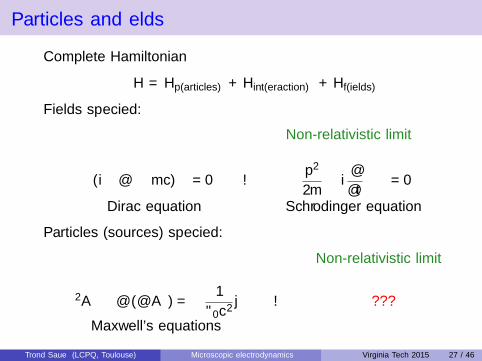
Particles and fields

Complete Hamiltonian

H = Hp(articles) + Hint(eraction) + Hf(ields)

Fields specified:

Non-relativistic limit

(iγµ∂µ −mc)ψ = 0 →(

p2

2m− i

∂

∂t

)ψ = 0

Dirac equation Schrodinger equation

Particles (sources) specified:

Non-relativistic limit

�2Aµ − ∂µ(∂νAν) = − 1

ε0c2jµ → ???

Maxwell’s equations


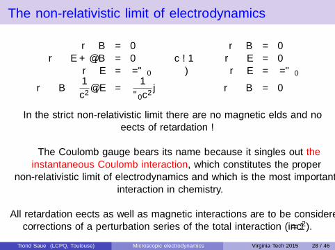
The non-relativistic limit of electrodynamics

∇ · B = 0 ∇ · B = 0∇× E + ∂tB = 0 c →∞ ∇× E = 0

∇ · E = ρ/ε0 ⇒ ∇ · E = ρ/ε0

∇× B− 1

c2∂tE =

1

ε0c2j ∇× B = 0

In the strict non-relativistic limit there are no magnetic fields and noeffects of retardation !

The Coulomb gauge bears its name because it singles out theinstantaneous Coulomb interaction, which constitutes the proper

non-relativistic limit of electrodynamics and which is the most importantinteraction in chemistry.

All retardation effects as well as magnetic interactions are to be consideredcorrections of a perturbation series of the total interaction (in 1/c2).


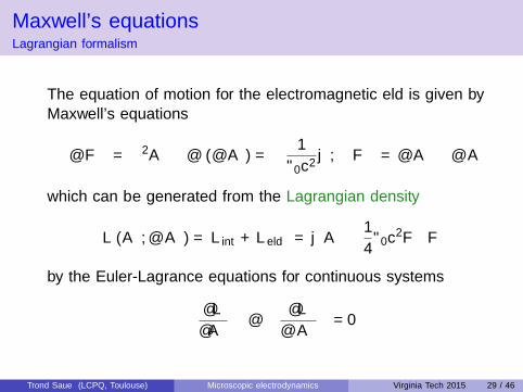
Maxwell’s equationsLagrangian formalism

The equation of motion for the electromagnetic field is given byMaxwell’s equations

∂νFνµ = �2Aµ − ∂µ (∂νAν) = − 1

ε0c2jµ; Fνµ = ∂νAµ − ∂µAµ

which can be generated from the Lagrangian density

L (Aα, ∂βAα) = Lint + Lfield = jαAα −1

4ε0c

2FαβFαβ

by the Euler-Lagrance equations for continuous systems

∂L∂Aα

− ∂β(

∂L∂βAα

)= 0


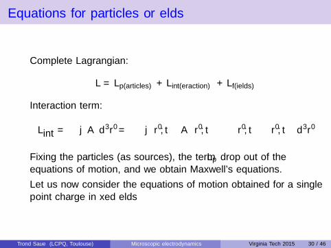
Equations for particles or fields

Complete Lagrangian:

L = Lp(articles) + Lint(eraction) + Lf(ields)

Interaction term:

Lint =

ˆjµAµd

3r′ =

ˆ [j(r′, t)· A(r′, t)− ρ

(r′, t)φ(r′, t)]

d3r′

Fixing the particles (as sources), the term Lp drop out of theequations of motion, and we obtain Maxwell’s equations.

Let us now consider the equations of motion obtained for a singlepoint charge in fixed fields


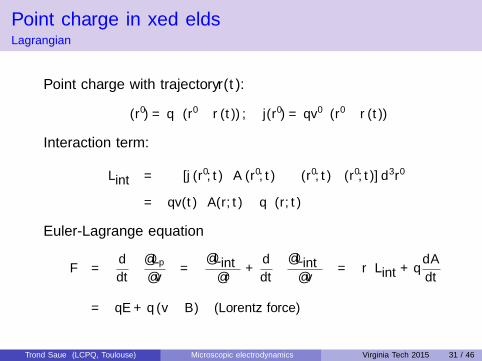
Point charge in fixed fieldsLagrangian

Point charge with trajectory r(t):

ρ(r′) = qδ (r′ − r (t)) ; j(r′) = qv′δ (r′ − r (t))

Interaction term:

Lint =

ˆ[j (r′, t) · A (r′, t)− ρ (r′, t)φ (r′, t)] d3r′

= qv(t) · A(r, t)− qφ(r, t)

Euler-Lagrange equation

F =d

dt

(∂Lp

∂v

)= −

∂Lint∂r

+d

dt

(∂Lint∂v

)= −∇Lint + q

dA

dt

= qE + q (v × B) (Lorentz force)


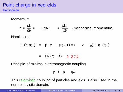
Point charge in fixed fieldsHamiltonian

Momentum

p =∂L

∂v= π + qA; π =

∂Lp

∂v(mechanical momentum)

Hamiltonian

H (r,p, t) = p · v − L (r, v, t) = (π · v − Lp) + qφ(r, t)

= Hp (r,π, t) + qφ(r, t)

Principle of minimal electromagnetic coupling

pµ → pµ − qAµ

This relativistic coupling of particles and fields is also used in thenon-relativistic domain.


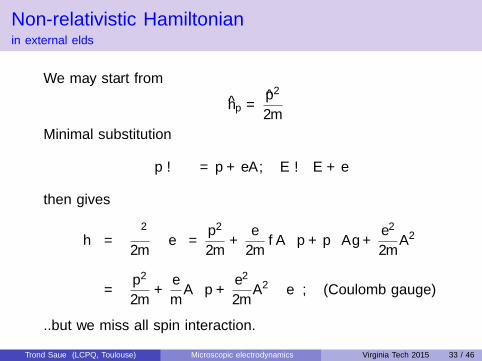
Non-relativistic Hamiltonianin external fields

We may start from

hp =p2

2m

Minimal substitution

p→ π = p + eA; E → E + eφ

then gives

h =π2

2m− eφ =

p2

2m+

e

2m{A · p + p · A}+

e2

2mA2

=p2

2m+

e

mA · p +

e2

2mA2 − eφ; (Coulomb gauge)

..but we miss all spin interaction.


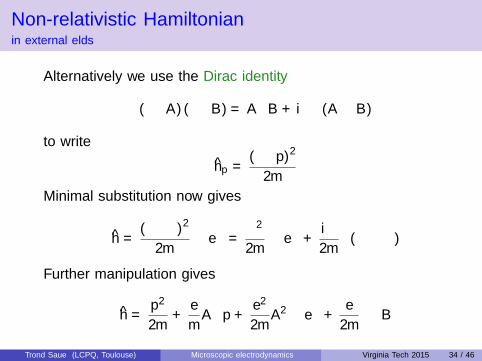
Non-relativistic Hamiltonianin external fields

Alternatively we use the Dirac identity

(σ · A) (σ · B) = A · B + iσ · (A× B)

to write

hp =(σ · p)2

2m

Minimal substitution now gives

h =(σ · π)2

2m− eφ =

π2

2m− eφ+

iσ

2m· (π × π)

Further manipulation gives

h =p2

2m+

e

mA · p +

e2

2mA2 − eφ+

e

2mσ · B


Energy flow


The Lorentz force and work

Lorentz force: force on the charge

F = qE + q(v × B)

Work on the charge

W =

ˆ r(tb)

r(ta)

F · dr =

ˆ tb

ta

(F · v) dt; v =dr

dt

Insertion of the Lorentz force gives

W =

ˆ tb

ta

(qE · v) dt +

ˆ tb

ta

q(v × B) · vdt =

ˆ tb

ta

(E · qv) dt +

ˆ tb

ta

q (v × v)︸︷︷︸=0

·Bdt

Magnetic forces do no work !

The substitution p→ π = p + eA corresponds to the removal of themagnetic contribution from the former.


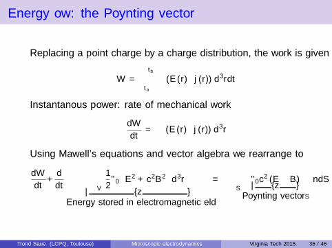
Energy flow: the Poynting vector

Replacing a point charge by a charge distribution, the work is given by

W =

ˆ tb

ta

ˆ(E (r) · j (r)) d3rdt

Instantanous power: rate of mechanical work

dW

dt=

ˆ(E (r) · j (r)) d3r

Using Mawell’s equations and vector algebra we rearrange to

dW

dt+

d

dt

{ˆV

1

2ε0(E 2 + c2B2

)d3r

}︸︷︷︸

Energy stored in electromagnetic field

= −ˆ

S

ε0c2 (E× B)︸︷︷︸

Poynting vector S

·ndS


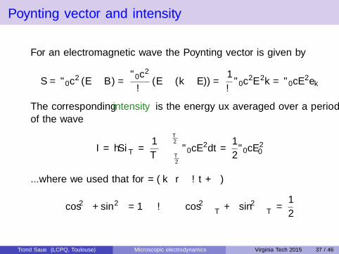
Poynting vector and intensity

For an electromagnetic wave the Poynting vector is given by

S = ε0c2 (E× B) =

ε0c2

ω(E× (k× E)) =

1

ωε0c

2E 2k = ε0cE2ek

The corresponding intensity is the energy flux averaged over a periodof the wave

I = 〈S〉T =1

T

ˆ T2

−T2

ε0cE2dt =

1

2ε0cE

20

...where we used that for θ = (k · r − ωt + δ)

cos2 θ + sin2 θ = 1 →⟨cos2 θ

⟩T

+⟨sin2 θ

⟩T

=1

2


Multipolar gauge


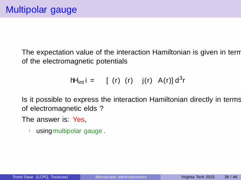
Multipolar gauge

The expectation value of the interaction Hamiltonian is given in termsof the electromagnetic potentials

〈Hint〉 =

ˆ[ρ(r)φ(r)− j(r) · A(r)] d3r

Is it possible to express the interaction Hamiltonian directly in termsof electromagnetic fields ?

The answer is: Yes,

I using multipolar gauge.


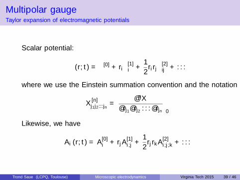
Multipolar gaugeTaylor expansion of electromagnetic potentials

Scalar potential:

φ (r, t) = φ[0] + riφ[1]i +

1

2ri rjφ

[2]ij + . . .

where we use the Einstein summation convention and the notation

X[n]j1j2...jn

=∂nX

∂rj1∂rj2 . . . ∂rjn

∣∣∣∣0

Likewise, we have

Ai (r, t) = A[0]i + rjA

[1]i ;j +

1

2rj rkA

[2]i ;j ,k + . . .


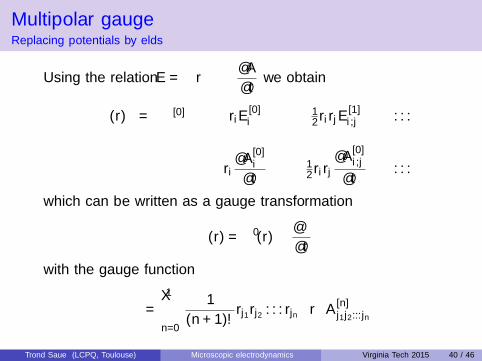
Multipolar gaugeReplacing potentials by fields

Using the relation E = −∇φ− ∂A

∂twe obtain

φ(r) = φ[0] − riE[0]i − 1

2 ri rjE[1]i ;j − . . .

− ri∂A

[0]i

∂t− 1

2 ri rj∂A

[0]i ;j

∂t− . . .

which can be written as a gauge transformation

φ(r) = φ′(r)− ∂χ

∂t

with the gauge function

χ =∞∑

n=0

1

(n + 1)!rj1rj2 . . . rjn

(r · A[n]

j1j2...jn

)Trond Saue (LCPQ, Toulouse) Microscopic electrodynamics Virginia Tech 2015 40 / 46

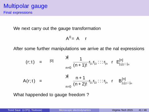
Multipolar gaugeFinal expressions

We next carry out the gauge transformation

A′ = A−∇χ

After some further manipulations we arrive at the final expressions

φ(r, t) = φ[0] −∞∑

n=0

1

(n + 1)!rj1rj2 . . . rjn

(r · E[n]

j1j2...jn

)

A(r, t) = −∞∑

n=0

n + 1

(n + 2)!rj1rj2 . . . rjn

(r × B

[n]j1j2...jn

)What happended to gauge freedom ?


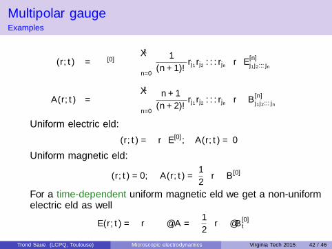
Multipolar gaugeExamples

φ(r, t) = φ[0] −∞∑

n=0

1

(n + 1)!rj1rj2 . . . rjn

(r · E[n]

j1j2...jn

)

A(r, t) = −∞∑

n=0

n + 1

(n + 2)!rj1rj2 . . . rjn

(r × B

[n]j1j2...jn

)Uniform electric field:

φ(r, t) = −r · E[0]; A(r, t) = 0

Uniform magnetic field:

φ(r, t) = 0; A(r, t) =1

2

(r × B[0]

)For a time-dependent uniform magnetic field we get a non-uniformelectric field as well

E(r, t) = −∇φ− ∂tA = −1

2

(r × ∂B

[0]t


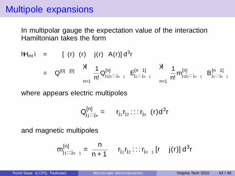
Multipole expansions

In multipolar gauge the expectation value of the interactionHamiltonian takes the form

〈Hint〉 =

ˆ[ρ(r)φ(r)− j(r) · A(r)] d3r

= Q [0]φ[0] −∞∑

n=1

1

n!Q

[n]j1j2...jn−1

· E[n−1]j1...jn−1

−∞∑

n=1

1

n!m

[n]j1j2...jn−1

· B[n−1]j1...jn−1

where appears electric multipoles

Q[n]j1...jn

=

ˆrj1rj2 . . . rjnρ(r)d3r

and magnetic multipoles

m[n]j1...jn−1

=n

n + 1

ˆrj1rj2 . . . rjn−1 [r × j(r)] d3r


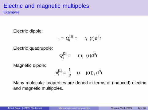
Electric and magnetic multipolesExamples

Electric dipole:

µi = Q[1]i =

ˆriρ(r)d3r

Electric quadrupole:

Q[2]ij =

ˆri rjρ(r)d3r

Magnetic dipole:

m[1]i =

1

2

ˆ(r × j(r))i d

3r

Many molecular properties are defined in terms of (induced) electricand magnetic multipoles.


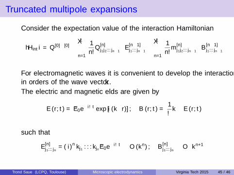
Truncated multipole expansions

Consider the expectation value of the interaction Hamiltonian

〈Hint〉 = Q [0]φ[0] −∞∑

n=1

1

n!Q

[n]j1j2...jn−1

· E[n−1]j1...jn−1

−∞∑

n=1

1

n!m

[n]j1j2...jn−1

· B[n−1]j1...jn−1

For electromagnetic waves it is convenient to develop the interactionin orders of the wave vector k.

The electric and magnetic fields are given by

E (r, t) = E0e−iωt exp [i (k · r)] ; B (r, t) =

1

ωk× E (r, t)

such that

E[n]j1...jn

= (i)n kj1 . . . kjn E0e−iωt ∼ O (kn) ; B

[n]j1...jn

∼ O(kn+1


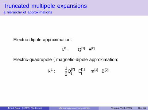
Truncated multipole expansionsa hierarchy of approximations

Electric dipole approximation:

k0 : −Q[1] · E[0]

Electric-quadrupole – magnetic-dipole approximation:

k1 : −1

2Q

[2]j · E

[1]j −m[1] · B[0]


Microscopic electrodynamics - Virginia Tech€¦ · Continuity equation r B 1 c2 @ tE = 0j r(r ......

Documents

Transcript of Microscopic electrodynamics - Virginia Tech€¦ · Continuity equation r B 1 c2 @ tE = 0j r(r ......