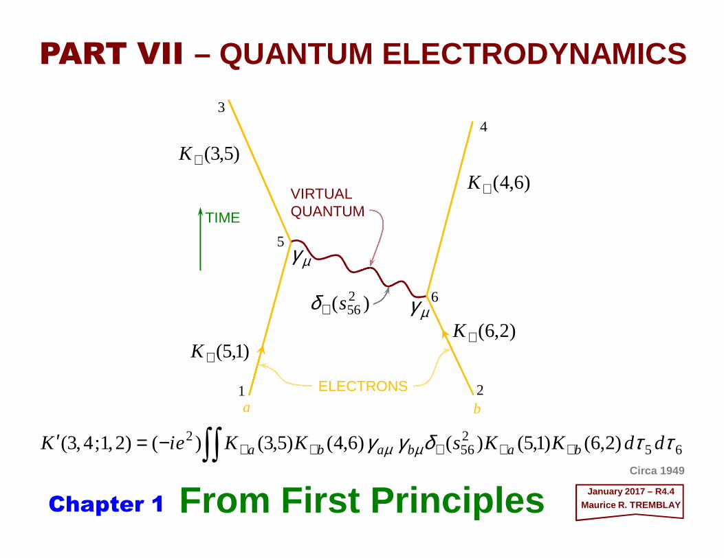
From First Principles January 2017 – R4.4Maurice R. TREMBLAY

PART VII – QUANTUM ELECTRODYNAMICS

∫∫ +++++−=′ 65256

2 )2,6()1,5()()6,4()5,3()()2,1;4,3( ττδγγ µµ ddKKsKKeiK bababa

ELECTRONS

VIRTUAL QUANTUMTIME

1 2

34

5

6)( 256s+δ

)6,4(+K

)1,5(+K)2,6(+K

)5,3(+K

µγ

µγ

a b

Circa 1949

Chapter 1

The cover picture is a Feynman diagram which shows the interaction between two elec-trons that end up with the exchange of a virtual quantum between both electrons. Every physics enthusiast knows about them but do they really understand where they come from or how they are generated? Graduate students are well acquainted with them in prac-tical calculations that they have to do in any Particle Physics course. It is one of those tools that is useful in quantum electrodynamics calculations because the fine structure constant is 1/137which allows perturbative techniques to be used. Thus, R.P. Feynman innovated by developing a set of rules using such diagrams to help in those calculations.

Now, although we have already touched on the subject of Dirac’s relativistic theory of the electron in PART IV – QUANTUM FIELDS , here we will revisit it but with the theoreti-cal physicist to be in mind. Maxwell’s theory will be reviewed and quantization will alsobe done but this time over all of space-time. The goal will be to show how electrons and photons interact using quantum fields set up as operators stemming from a decomposi-tion in terms of Fourier modes using an idealized harmonic oscillator approximation.

2Forward

2017MRT

As with my other work, nothing of this is new or even developed first hand and frankly it is a rearranged compilation of various quotes from various sources (c.f., References) that aims to display an abridged but yet concise and straightforward mathematical development of quantum electrodynamics as I have understood it and wish it to be presented to the layman or to the inquisitive person. Now, as a matter of convention, this time I will use natural units in which we set h≡c≡1 in most of the equations and ancillary theoretical discussions and I also use the summation convention that does imply the summation over any repeated indices (typically subscript-superscript) in an equation.

Now, this set of slides is a bit different than the others. I have plagiarized Sakurai’s and Kaku’s prose to the point of feeling bad about it but I think the point will be to have you read through these time and time again until the formulation and steps leading to quan-tum electrodynamics becomes so inherent that you can figure out what the next steps are for yourself. It is a bit of a learning tactic if you will – that is, have you figure things out by either learning it first hand or having you dig it out for you to understand it clearly! So, I will not hide the fact from you that the prose used here is pretty much what you would get verbatim if you were to have to sit down in a lecture hall at the City College of New York or have to look at a YouTube recording of the guy (e.g., Prof. Michio Kaku).

3

2017MRT

As for the content, I have to be honest… The critical path to get you to the goal of find-ing out how Feynman diagrams come together is the best I’ve seen or read about! I think it is the point of Kaku’s book – lecture notes and problems in one volume! These slides then serve as an everlasting homage to Kaku’s first exposure to QED… Either you get it or you have to work for it! But, as a whole, all of this is definitely from first principles.

One last thing. The true goal of this set of slides is to show you how physics concepts can come together to define such a thing as the interaction of electrons with photons and as I once said: “You have to be in love with quantum field theory to understand it! How else can you read each line, paragraph and chapter again and again with such devotion.” In the end, what counts is that you gain some knowledge about the real world that surrounds you and maybe if you are keen enough you will appreciate sunlight better afterwards as it may – unbeknownst to your visual acuity – perform a dance of virtualparticles for you to ponder on as you get a tan outside during those nice summer days.

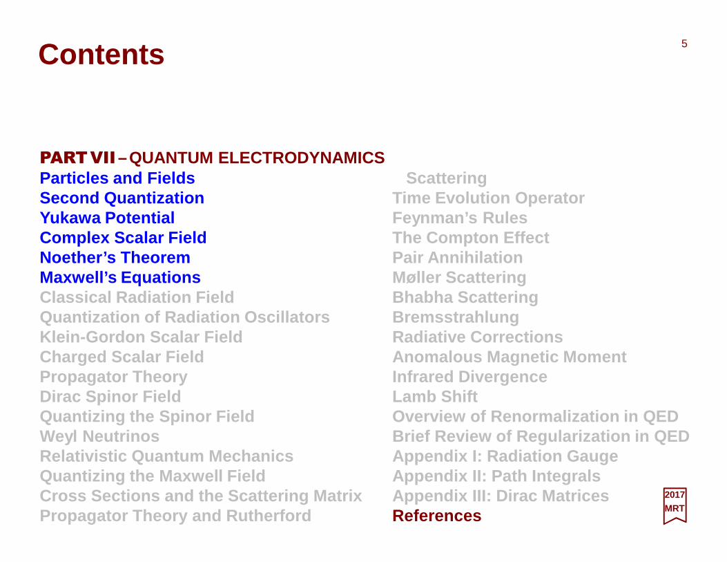
Contents of 3-Chapter PART VII

PARTVII–QUANTUM ELECTRODYNAMICSParticles and FieldsSecond QuantizationYukawa PotentialComplex Scalar FieldNoether’s TheoremMaxwell’s EquationsClassical Radiation FieldQuantization of Radiation OscillatorsKlein-Gordon Scalar FieldCharged Scalar FieldPropagator TheoryDirac Spinor FieldQuantizing the Spinor FieldWeyl NeutrinosRelativistic Quantum MechanicsQuantizing the Maxwell FieldCross Sections and the Scattering MatrixPropagator Theory and Rutherford

2017MRT

4

ScatteringTime Evolution OperatorFeynman’s RulesThe Compton EffectPair AnnihilationMøller ScatteringBhabha ScatteringBremsstrahlungRadiative CorrectionsAnomalous Magnetic MomentInfrared DivergenceLamb ShiftOverview of Renormalization in QEDBrief Review of Regularization in QEDAppendix I: Radiation GaugeAppendix II: Path IntegralsAppendix III: Dirac MatricesReferences

“…hardly anything has been done up to the present on quantum electrodynamics. The question of the correct treatment of a system in which the forces a re propagated with the velocity of light instead of instantaneously, of the production of an electromag netic field by a moving electron, and of the reacti on of this field on the electron have not yet been touche d.” Paul Dirac, Proc. Roy. Soc. Lon. A114, 243 (1927).

Contents

PARTVII–QUANTUM ELECTRODYNAMICSParticles and FieldsSecond QuantizationYukawa PotentialComplex Scalar FieldNoether’s TheoremMaxwell’s EquationsClassical Radiation FieldQuantization of Radiation OscillatorsKlein-Gordon Scalar FieldCharged Scalar FieldPropagator TheoryDirac Spinor FieldQuantizing the Spinor FieldWeyl NeutrinosRelativistic Quantum MechanicsQuantizing the Maxwell FieldCross Sections and the Scattering MatrixPropagator Theory and Rutherford

2017MRT

5

ScatteringTime Evolution OperatorFeynman’s RulesThe Compton EffectPair AnnihilationMøller ScatteringBhabha ScatteringBremsstrahlungRadiative CorrectionsAnomalous Magnetic MomentInfrared DivergenceLamb ShiftOverview of Renormalization in QEDBrief Review of Regularization in QEDAppendix I: Radiation GaugeAppendix II: Path IntegralsAppendix III: Dirac MatricesReferences

2017MRT

Nonrelativistic quantum mechanics (c.f.,PART III – QUANTUM MECHANICS ), developed in the years from 1923 to 1926, provides a unified and logically consistent picture of numerous phenomena in the atomic and molecular domain. Following P. A. M. Dirac, we might be tempted to assert: “The underlying physical laws necessary for the mathema-tical theory of a large part of physics and the whole of chemistry are completely known.”

Particles and Fields

There are, however, basically two reasons for believing that the description of physical phenomena based on nonrelativistic quantum mechanics is incomplete. First, since nonrelativistic quantum mechanics is formulated in such a way as to yield the nonrelati-vistic energy-momentum relation in the classical limit (i.e., T=½mv2=p2/2m with vector momentum p=mv), it is incapable of accounting for the fine structure of a hydrogen-like atom (c.f., PART V – THE HYDROGEN ATOM ). (N.B., This problem was also treated even earlier by A. Sommerfeld, who used a relativistic generalization of N. Bohr’s atomic model). In general, nonrelativistic quantum mechanics makes no prediction about the dynamical behavior of (point) particles moving at relativistic velocities. This defect was amended by the relativistic theory of electrons developed by Dirac in 1928, which was discussed in PART IV – QUANTUM FIELDS . Second, and what is more serious, nonrelativistic quantum mechanics is essentially a single-particle theory in which the probability density for finding a given particle integrated over all space is unity at all times. Thus it is not constructed to describe phenomena such as nuclear beta decay in which an electron and an antineutrino are created as the neutron becomes a proton or to describe even a simpler process in which an excited atom returns to its ground state by spontaneously emitting a single photon in the absence of any external field.

6

The major part of these slides is devoted to the progress physicists have made since the historic 1927 paper of Dirac’s entitled: “The Quantum Theory of the Emission and Absorption of Radiation” opened up a new subject called the quantum theory of fields.

Now, the concept of a field was originally introduced in classical physics to account for the interaction between two bodies separated by a finite distance. In classical physics (c.f., PART II – MODERN PHYSICS) the electric (vector) field E(x,t), for instance, is a three-component function E defined at each space-time point [x,t], and the interactionbetween two charged bodies, 1 and 2, is to be viewed as the interaction of body 2 with the electrical field created by body 1. In the quantum theory, however, the field concept acquires a new dimension. As originally formulated in the late 1920s and early 1930s, the basic idea of quantum field theory is that we associate particles with fields such as the electromagnetic field! To put it more precisely, quantum-mechanical excitations of a field appear as particles of definite mass and spin (c.f., PART VI – GROUP THEORY).

7

2017MRT

Even before the advent of post WWII calculational techniques which enabled us to compute quantities such as the 2S½-2P½ separation of the Hydrogen atom to an accuracy of one part in 108, there had been a number of brilliant successes of the quantum theory of fields. First, the quantum theory of radiation developed by Dirac and others provides quantitative understandings of a wide class of phenomena in which real photons are emitted or absorbed. Second, the requirements imposed by quantum field theory, when combined with other general principles such as Lorentz invariance and the probabilistic interpretation of state vectors, severely restrict the class of (point-like) particles that are permitted to exist in nature (i.e., in space-time).

In particular, we may cite the following two rules derivable from relativistic quantum field theory: 1) For every charged particle there must exist an antiparticle with opposite charge and with the same mass and lifetime; 2) The particles that occur in nature must obey the spin-statistics theorem (N.B., first proved by W. Pauli in 1940) which states that (in units of h): i. half-integer spin particles (e.g., electron, proton, Λ-hyperon) must obey Fermi-Dirac statistics, whereas ii. integer spin particles (e.g., photon, π-meson, K-meson) must obey Bose-Einstein statistics. Empirically there is no known exception to these rules; and 3) The existence of a nonelectromagnetic interaction between two nucleons at short but finite distances prompts us to infer that a field is responsible for nuclear forces; this, in turn, implies the existence of massive particles associated with the field, a point first emphasized by H. Yukawa in 1935 (c.f., Yukawa Potential chapter), and as is well known, the desired particles, now known asπ-mesons or pions, were found experimentally twelve years after the theoretical prediction of their existence. Woo-hoo!

These considerations appear to indicate that the idea of associating particles with fields and, conversely, fields with particles is not entirely wrong. There are, however, difficulties with the present form of quantum field theory which must be overcome in the future... First, despite the striking success of postwar quantum electrodynamics (QED) in calcula-ting various observable effects, the unobservable modifications in the mass and charge of the electron due to the emission and reabsorption of a virtual photon turns out to diverge logarithmically with the frequency of the virtual photon (i.e., QED contains integrals that diverge as x→0, or, in momentum space, as k→∞).These divergences reflected our ignorance concerning the small-scale (i.e., x→0) structure of space-time.

8

2017MRT

Second, the idea of associating a field with each particle observed in nature becomes ridiculous and distasteful when we consider the realm of strong interactions where many different kinds of particles are known to interact with one another; we know from experiment that nearly 100 particles or resonances participate in the physics of strong interactions (to check on the very latest, c.f., Particle Data Group at http://pdg.lbl.gov/).

Nevertheless, quantum field theory has emerged as the most successful physical framework describing the subatomic world. Both its computational power and its conceptual scope are remarkable. Its predictions for the interactions between electrons and photons have proved to be correct to within one part in 108. Furthermore, it can adequately explain the interactions of three of the four known fundamental forces in the universe. The success of quantum field theory as a theory of subatomic forces is today embodiedinwhat is called the Standard Model (c.f.,PART VIII–THESTANDARD MODEL– with the most current research being done at CERN at http://home.web.cern.ch/about/).

9

2017MRT

In this set of slides, we somewhat go on a tangent and explore QED by formulating the correct theory of the electron-photon system and this will lead us to understand why QED is a theory that has been found to be so successful experimentally to a very high degree (e.g., the electron’s anomalous magnetic moment) but we will also close the gap in learning between PART III-VI and PART VIII such as to allow the interested reader to delve right here into formulations that otherwise might appear opaque as to their presence or the reason for their inclusion in the preamble content necessary to explain the formulation of the Standard Model. On the other hand, a quick perusal of the first hundred or so slides might just as well do as a primer or refresher in QED…

10

2017MRT

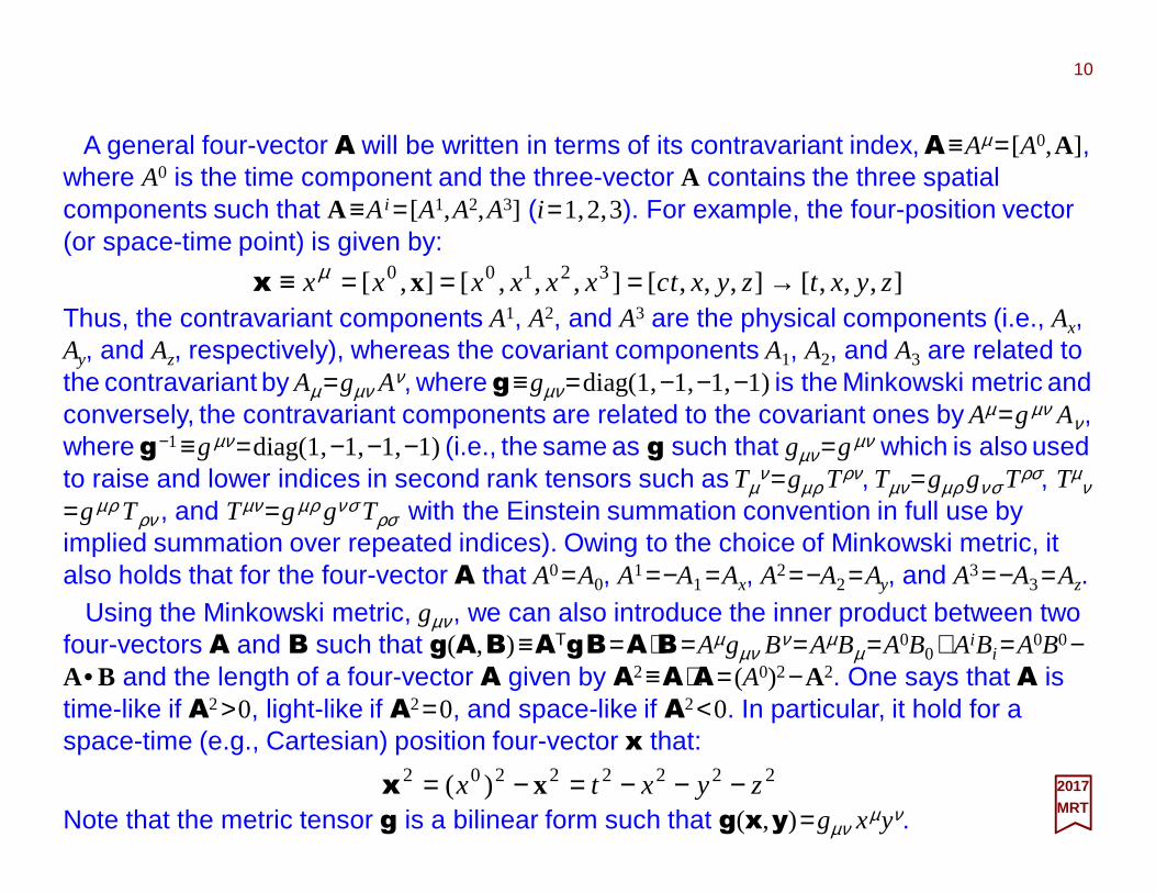
A general four-vector A will be written in terms of its contravariant index,A≡Aµ = [A0,A], where A0 is the time component and the three-vector A contains the three spatialcomponents such that A ≡Ai = [A1,A2,A3] (i =1,2,3). For example, the four-position vector (or space-time point) is given by:

Using the Minkowski metric, gµν , we can also introduce the inner product between two four-vectors A and B such that g(A,B)≡ATgB=A⋅B=Aµgµν Bν =AµBµ =A0B0+AiBi =A0B0−A•B and the length of a four-vector A given by A2≡A⋅A= (A0)2−A2. One says that A is time-like if A2>0, light-like if A2=0, and space-like if A2<0. In particular, it hold for a space-time (e.g., Cartesian) position four-vector x that:

Note that the metric tensor g is a bilinear form such that g(x,y)=gµν xµyν.

22222202 )( zyxtx −−−=−= xx

Thus, the contravariant components A1, A2, and A3 are the physical components (i.e., Ax, Ay, and Az, respectively), whereas the covariant components A1, A2, and A3 are related to the contravariant by Aµ =gµν Aν, whereg≡gµν=diag(1,−1,−1,−1) is the Minkowski metric and conversely, the contravariant components are related to the covariant ones by Aµ =gµν Aν, whereg−1≡gµν =diag(1,−1,−1,−1) (i.e., the same as g such that gµν =gµν which is also used to raise and lower indices in second rank tensors such as Tµ

ν =gµρ Tρν, Tµν=gµρ gνσ Tρσ, Tµν

=gµρ Tρν , and Tµν =gµρ gνσ Tρσ with the Einstein summation convention in full use by implied summation over repeated indices). Owing to the choice of Minkowski metric, it also holds that for the four-vector A that A0=A0, A1=−A1=Ax, A2=−A2=Ay, and A3=−A3=Az.

],,,[],,,[],,,[],[ 32100 zyxtzyxtcxxxxxx →===≡ xµx

11

2017MRT

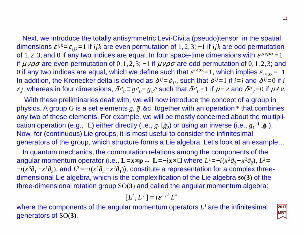
Next, we introduce the totally antisymmetric Levi-Civita (pseudo)tensor in the spatial dimensions ε i jk =ε i jk =1 if i jk are even permutation of 1,2,3; −1 if i jk are odd permutation of 1,2,3; and 0 if any two indices are equal. In four space-time dimensions with ε µνρσ =1if µνρσ are even permutation of 0,1,2,3; −1 if µνρσ are odd permutation of 0,1,2,3; and 0 if any two indices are equal, which we define such that ε 0123=1, which implies ε 0123=−1. In addition, the Kronecker delta is defined as δ ij =δ i j , such that δ ij =1 if i = j and δ i j =0 if i≠ j, whereas in four dimensions, δ µ

ν ≡ gµν = gν

µ such that δ µν =1 if µ =ν and δ µ

ν =0 if µ ≠ν.

In quantum mechanics, the commutation relations among the components of the angular momentum operator (i.e., L =x××××p↔ L =−ix××××∇∇∇∇ where L1=−i (x2∂3−x3∂2), L2=−i (x3∂1−x1∂3), and L3=−i (x1∂2−x2∂1)), constitute a representation for a complex three-dimensional Lie algebra, which is the complexification of the Lie algebra so(3) of the three-dimensional rotation group SO(3) and called the angular momentum algebra:

kkjiji LiLL ε=],[where the components of the angular momentum operators L i are the infinitesimal generators of SO(3).

With these preliminaries dealt with, we will now introduce the concept of a group in physics. A group G is a set elements g, g,&c. together with an operation * that combinesany two of these elements. For example, we will be mostly concerned about the multipli-cation operation (e.g., ‘ ⋅ ’) either directly (i.e., g1⋅g2) or using an inverse (i.e., g1

−1⋅g2). Now, for (continuous) Lie groups, it is most useful to consider the infinitesimal generators of the group, which structure forms a Lie algebra. Let’s look at an example…

−

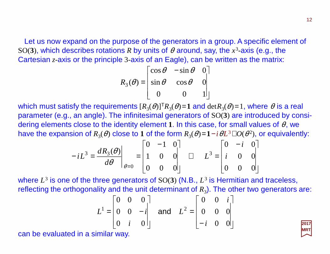
Let us now expand on the purpose of the generators in a group. A specific element of SO(3), which describes rotations R by units of θ around, say, the x3-axis (e.g., the Cartesian z-axis or the principle 3-axis of an Eagle), can be written as the matrix:

12

2017MRT

−=

100

0cossin

0sincos

)(3 θθθθ

θR

which must satisfy the requirements [R3(θ)]TR3(θ)=1 and detR3(θ )=1, where θ is a real parameter (e.g., an angle). The infinitesimal generators of SO(3) are introduced by consi-dering elements close to the identity element 1. In this case, for small values of θ , we have the expansion of R3(θ ) close to 1 of the form R3(θ )=1− iθL3+O(θ 2), or equivalently:

−=⇔

−==−

= 000

00

00

000

001

010)( 3

0

33 i

i

Ld

RdLi

θθθ

where L3 is one of the three generators of SO(3) (N.B., L3 is Hermitian and traceless, reflecting the orthogonality and the unit determinant of R3). The other two generators are:

−=

−=00

000

00

00

00

00021

i

i

L

i

iL and

can be evaluated in a similar way.

Now, we can exponentiate the operators L1, L2, and L3 in order to obtain unitary one-parameter groups. For example, let us study the one-parameter group generated by the operator L3. Introducing polar coordinates [θ,ϕ ] and taking ϕ as the polar angle in the x1x2-plane, we find that:

13

2017MRT

L++∂−−= )()()( 23 θθθ ϕ OiiR 1

which means that R3(θ ), via the application of the generator L3 on the angle θ , translates the angle ϕ by the amount −θ (i.e., using Taylor’s theorem above), that is, a clockwiserotation in the x1x2-plane by the angle θ . In general, for an arbitrary rotation, we obtain:

ˆwhere n is a unit vector pointing in an arbitrary direction.

Lnn

•−= ˆˆ e)( θθ iR

Therefore, we have (i.e., using R3(θ )=1− iθL3+O(θ 2) above): ϕ∂−= iL3

L+∂+∂−= 22

3 )(2

)( ϕϕθθθ 1R

or, when the imaginary unit i=√−1 is multiplied, we have:

3

e)(!

)()(

03

Li

N

nN

NR θ

ϕθθ −

∞

=

≡∂−=∑

which represents a series in ∂ϕ for which there is a convenient sum,and that sum is equi-valent to an imaginary exponential, in this case along the x3-axis, of the generator L3:

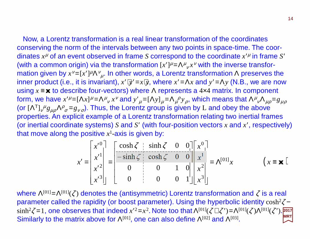
Now, a Lorentz transformation is a real linear transformation of the coordinates conserving the norm of the intervals between any two points in space-time. The coor-dinates xµ of an event observed in frame Scorrespond to the coordinate x′µ in frame S′(with a common origin) via the transformation [x′]µ=Λµ

ν xν with the inverse transfor-mation given by xν = [x′]µΛν

µ. In other words, a Lorentz transformation Λ preserves the inner product (i.e., it is invariant), x′⋅y′=x⋅y, where x′=Λx and y′=Λy (N.B., we are now using x ≡x to describe four-vectors) where Λ represents a 4×4 matrix. In component form, we have x′µ = [Λx] µ =Λµ

ν xν and y′µ = [Λy] µ =Λµρ yρ, which means that Λµ

ν Λµρ =gµρ(or [ΛT]ν

µgµρ Λρσ =gν σ). Thus, the Lorentz group is given by L and obey the above

properties. An explicit example of a Lorentz transformation relating two inertial frames (or inertial coordinate systems) Sand S′ (with four-position vectors x and x′, respectively) that move along the positive x1-axis is given by:

14

2017MRT

x

x

x

x

x

x

x

x

x

x ]01[

3

2

1

0

3

2

1

0

1000

0100

00coshsinh

00sinhcosh

Λ=

−=

′′′′

=′ζζζζ

where Λ[01]=Λ[01](ζ ) denotes the (antisymmetric) Lorentz transformation and ζ is a real parameter called the rapidity (or boost parameter). Using the hyperbolic identity cosh2ζ −sinh2ζ =1, one observes that indeed x′2=x2. Note too that Λ[01](ζ +ζ ′)=Λ[01](ζ )Λ[01](ζ ′). Similarly to the matrix above for Λ[01], one can also define Λ[02] and Λ[03].

( )x≡x

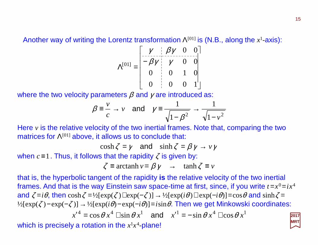
Another way of writing the Lorentz transformation Λ[01] is (N.B., along the x1-axis):

15

2017MRT

−=Λ

1000

0100

00

00

]01[ γγβγβγ

where the two velocity parameters β and γ are introduced as:

22 1

1

1

1

vv

c

v

−→

−≡→≡

βγβ and

Here v is the relative velocity of the two inertial frames. Note that, comparing the two matrices for Λ[01] above, it allows us to conclude that:

when c≡1. Thus, it follows that the rapidity ζ is given by:γγβζγζ v→== sinhcosh and

vv ≡→=≡ ζγβζ tanharctanh

that is, the hyperbolic tangent of the rapidity is the relative velocity of the two inertial frames. And that is the way Einstein saw space-time at first, since, if you write t =x0= ix4

and ζ = iθ, then coshζ =½[exp(ζ )+exp(−ζ )] →½[exp(iθ )+ exp(−iθ)] =cosθ and sinhζ =½[exp(ζ )−exp(−ζ )] →½[exp(iθ)−exp(−iθ)] = isinθ. Then we get Minkowski coordinates:

which is precisely a rotation in the x1x4-plane!

141144 cossinsincos xxxxxx θθθθ +−=′+=′ and

The physical interpretation of the above is as follows… A particle (or an observer O) at rest in the inertial frame S is represented by a world-line parallel to the time axis (i.e., the x0-axis). Let us assume that O is at rest at the origin of the three-dimensional space in S. The same observer O can also be viewed from another inertial frame S′, which is related to Sby the Lorentz transformation Λ[01]. In the S′-coordinates, the world-line of O is given by x′0=τ coshζ, x′1=−τ sinhζ, and x′2=x′3=0, where we have used x0=τ and x1=x2=x3= 0 for the S-coordinates.The velocity of O along the x′1-axis is now v′=dx′1/dt′ =−tanhζ ≤0whereas the velocityalong the other axes is zero.Thus,we can interpret this result aseither:1. O (or a particle with rest mass) is moving with velocity −v′ along the negative x′1-axis; or 2. S′ is movingwith velocity v′ =dx1/dt = tanhζ ≤0along the positive x1-axis. Note that v′=−v.

16

2017MRT

and (Λ00)2=1+Σi(Λ0

i)2≥1 (i.e., Λ00≥1 or Λ0

0≤−1). The four conditions detΛ=±1, Λ00≥1,

and Λ00≤1 can be used to classify the elements of the Lorentz group L (i.e., SO(3,1) in

group theory). Thus we can divide the Lorentz group L into the following subgroups: 1. The proper Lorentz group L+ with detΛ=1; 2. The orthochronous Lorentz group L with Λ0

0≥1; and 3. The proper and orthochronous Lorentz group L+ =L+ ∩L.We will only care about L+.

Now, using the inner product g(Λx,Λy)=Λx⋅Λy=x⋅y=g(x,y), we find that x⋅y=xTgy and Λx⋅Λy= (Λx)Tg(Λy)=xTΛTgΛy. These last two inner products are invariant under Lorentz transformations so as to imply that g=ΛTgΛ which is basically the same result obtained earlier but this time in matrix form. From this result, one obtains:

1det1)(det 2 ±=Λ=Λ or

~~ ~~

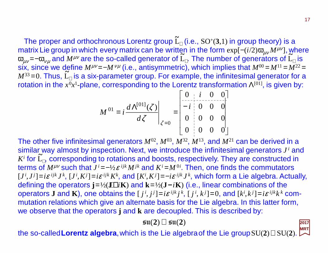
The proper and orthochronous Lorentz group L+ (i.e., SO+(3,1) in group theory) is a matrix Lie group in which every matrix can be written in the form exp[−(i /2)ωµν Mµν], where ωµν =−ων µ and Mµν are the so-called generator of L+. The number of generators of L+ is six, since we define Mµν =−M νµ (i.e., antisymmetric), which implies that M00= M11= M22=M33=0. Thus, L+ is a six-parameter group. For example, the infinitesimal generator for a rotation in the x0x1-plane, corresponding to the Lorentz transformation Λ[01], is given by:

17

2017MRT

~

~

~

~

−=Λ=

=0000

0000

000

000

)(

0

]01[01 i

i

d

diM

ζζ

ζ

The other five infinitesimal generators M02, M03, M32, M13, and M21 can be derived in a similar way almost by inspection. Next, we introduce the infinitesimal generators J i and K i for L+, corresponding to rotations and boosts, respectively. They are constructed in terms of Mµν such that J i =−½ε i jk M jk and K i =M 0i. Then, one finds the commutators [J i,J j ] = iε i jk J k, [J i,K j ] = iε i jk Kk, and [K i,K j ] =−iε i jk J k, which form a Lie algebra. Actually, defining the operators j =½(J++++ iK ) and k =½(J−−−− iK ) (i.e., linear combinations of the operators J and K ), one obtains the [ j i, j j ] = iε i jk j k, [ j i, k j ] =0, and [ki,k j ] = iε i jkk k com-mutation relations which give an alternate basis for the Lie algebra. In this latter form, we observe that the operators j and k are decoupled. This is described by:

~

the so-calledLorentz algebra ,which is the Lie algebraof the Lie groupSU(2)⊗SU(2).

)()( 22 susu ⊕

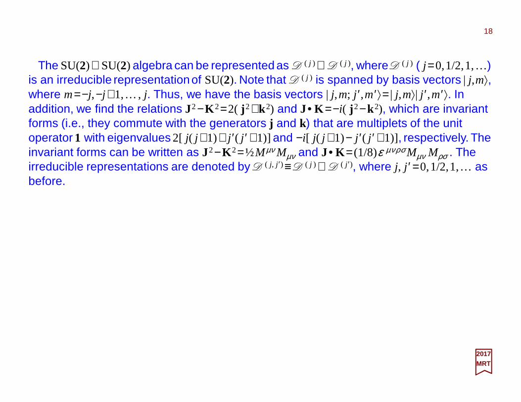
The SU(2)⊗SU(2) algebra can be represented as D ( j ) ⊗ D ( j ), where D ( j ) ( j =0,1/2,1,…) is an irreducible representationof SU(2). Note that D ( j ) is spanned by basis vectors | j,m⟩, where m=−j,−j +1,…, j. Thus, we have the basis vectors | j,m; j ′,m′⟩= | j,m⟩| j ′,m′⟩. In addition, we find the relations J2−K 2=2( j 2+k 2) and J•K =−i( j 2−k 2), which are invariant forms (i.e., they commute with the generators j and k) that are multiplets of the unit operator 1 with eigenvalues 2[ j( j +1)+ j ′( j ′+1)] and −i[ j( j +1)− j ′( j ′+1)], respectively. The invariant forms can be written as J2−K 2=½Mµν Mµν and J•K = (1/8)ε µνρσ Mµν Mρσ . The irreducible representations are denoted by D ( j, j ′) ≡ D ( j ) ⊗ D ( j ′), where j, j ′=0,1/2,1,…as before.

18

2017MRT

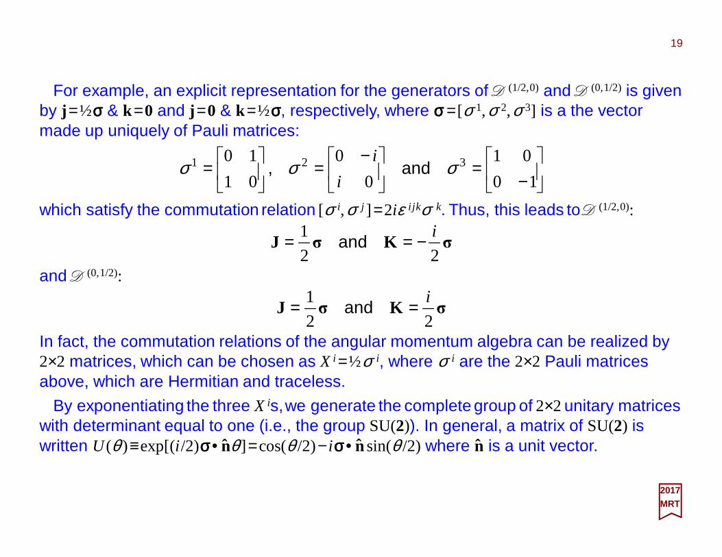
For example, an explicit representation for the generators of D (1/2,0) and D (0,1/2) is given by j =½σσσσ & k =0 and j =0 & k =½σσσσ, respectively, where σσσσ = [σ 1,σ 2,σ 3] is a the vector made up uniquely of Pauli matrices:

19

2017MRT

−=

−=

=

10

01

0

0

01

10 321 σσσ and,i

i

which satisfy the commutation relation [σ i,σ j ] =2iε i jkσ k. Thus, this leads to D (1/2,0):

In fact, the commutation relations of the angular momentum algebra can be realized by 2×2 matrices, which can be chosen as X i =½σ i, where σ i are the 2×2 Pauli matrices above, which are Hermitian and traceless.

σKσJ22

1 i−== and

and D (0,1/2):

σKσJ22

1 i== and

ˆˆˆ

By exponentiating the three X is,we generate the complete group of 2×2unitary matrices with determinant equal to one (i.e., the group SU(2)). In general, a matrix of SU(2) is written U (θ )≡exp[(i /2)σσσσ•nθ ] =cos(θ /2)− i σσσσ•nsin(θ /2) where n is a unit vector.

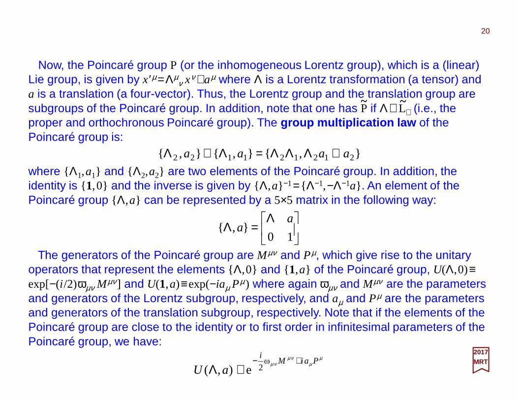
Now, the Poincaré group P (or the inhomogeneous Lorentz group), which is a (linear) Lie group, is given by x′µ=Λµ

ν xν +aµ where Λ is a Lorentz transformation (a tensor) and a is a translation (a four-vector). Thus, the Lorentz group and the translation group are subgroups of the Poincaré group. In addition, note that one has P if Λ∈L+ (i.e., the proper and orthochronous Poincaré group). The group multiplication law of the Poincaré group is:

20

2017MRT

~ ~

Λ=Λ

10},{

aa

The generators of the Poincaré group are Mµν and Pµ, which give rise to the unitary operators that represent the elements { Λ,0} and { 1,a} of the Poincaré group, U(Λ,0)≡exp[−(i /2)ωµν Mµν] and U(1,a)≡exp(−iaµ Pµ) where again ωµν and Mµν are the parameters and generators of the Lorentz subgroup, respectively, and aµ and Pµ are the parameters and generators of the translation subgroup, respectively. Note that if the elements of the Poincaré group are close to the identity or to first order in infinitesimal parameters of the Poincaré group, we have:

µµ

νµνµ PaiM

i

aU+−

≅Λω

2e),(

where { Λ1,a1} and { Λ2,a2} are two elements of the Poincaré group. In addition, the identity is { 1,0} and the inverse is given by { Λ,a} −1= { Λ−1,−Λ−1a} . An element of the Poincaré group { Λ,a} can be represented by a 5×5 matrix in the following way:

},{},{},{ 212121122 aaaa ⊕ΛΛΛ=Λ⊗Λ

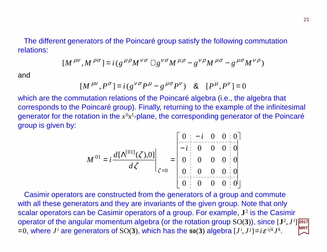
The different generators of the Poincaré group satisfy the following commutation relations:

21

2017MRT

−−

=Λ==

00000

00000

00000

0000

0000

]0),([

0

]01[01

i

i

d

diM

ζζ

ζ

Casimir operators are constructed from the generators of a group and commute with all these generators and they are invariants of the given group. Note that only scalar operators can be Casimir operators of a group. For example, J2 is the Casimir operator of the angular momentum algebra (or the rotation group SO(3)), since [J2,J i]=0, where J i are generators of SO(3), which has the so(3) algebra [J i,J j ] = iε i jk Jk.

which are the commutation relations of the Poincaré algebra (i.e., the algebra that corresponds to the Poincaré group). Finally, returning to the example of the infinitesimal generator for the rotation in the x0x1-plane, the corresponding generator of the Poincaré group is given by:

)(],[ ρνσµσµρνρµσνσνρµσρνµ MgMgMgMgiMM −−+=and

0],[)(],[ =−= νµνσµµσνσνµ PPPgPgiPM &

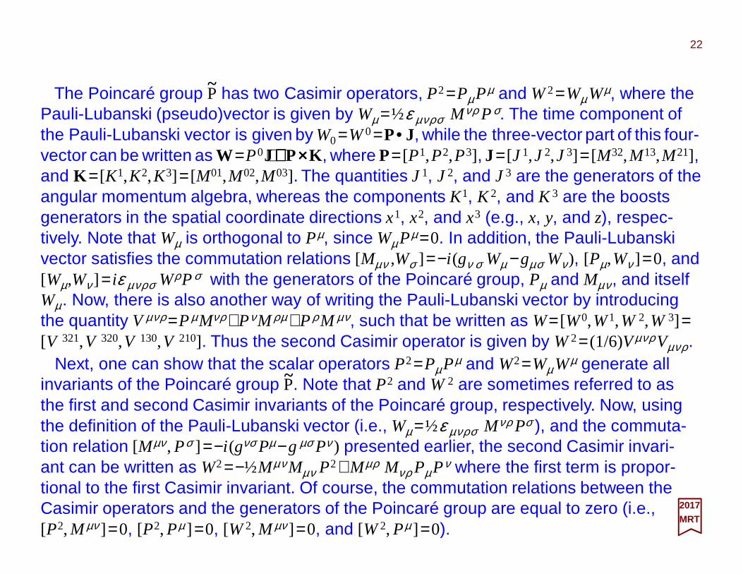
The Poincaré group P has two Casimir operators, P2=PµPµ and W2=Wµ Wµ, where the Pauli-Lubanski (pseudo)vector is given by Wµ =½ε µνρσ Mνρ Pσ. The time component of the Pauli-Lubanski vector is given by W0=W0=P•J, while the three-vector part of this four-vector can be written as W =P0J++++P××××K , where P= [P1,P2,P3], J= [J1,J 2,J 3] = [M32,M13,M21], and K = [K1,K2,K3] = [M01,M02,M03]. The quantities J 1, J 2, and J 3 are the generators of the angular momentum algebra, whereas the components K1, K 2, and K 3 are the boosts generators in the spatial coordinate directions x1, x2, and x3 (e.g., x, y, and z), respec-tively. Note that Wµ is orthogonal to Pµ, since Wµ Pµ =0. In addition, the Pauli-Lubanski vector satisfies the commutation relations [Mµν ,Wσ ] =−i (gν σ Wµ −gµσ Wν), [Pµ,Wν ] =0, and [Wµ,Wν ] = iε µνρσ WρPσ with the generators of the Poincaré group, Pµ and Mµν, and itself Wµ. Now, there is also another way of writing the Pauli-Lubanski vector by introducing the quantity V µνρ =PµMνρ +PνM ρµ +Pρ M µν, such that be written as W= [W0,W1,W2,W3] =[V 321,V 320,V 130,V 210]. Thus the second Casimir operator is given by W2= (1/6)Vµνρ Vµνρ.

22

2017MRT

Next, one can show that the scalar operators P2=PµPµ and W2=Wµ Wµ generate all invariants of the Poincaré group P. Note that P2 and W2 are sometimes referred to as the first and second Casimir invariants of the Poincaré group, respectively. Now, using the definition of the Pauli-Lubanski vector (i.e., Wµ =½ε µνρσ Mνρ Pσ ), and the commuta-tion relation [Mµν, Pσ ] =−i (gνσ Pµ −gµσ Pν ) presented earlier, the second Casimir invari-ant can be written as W2=−½MµνMµν P2+ Mµρ Mνρ PµPν where the first term is propor-tional to the first Casimir invariant. Of course, the commutation relations between the Casimir operators and the generators of the Poincaré group are equal to zero (i.e., [P2,M µν ] =0, [P2,Pµ ] =0, [W2, M µν ] =0, and [W2, Pµ ] =0).

~

~

A general problem when describing relativistic states is to find the meaning of the time parameter t and the position vector x in a wave function ΨΨΨΨ(x,t). Therefore, it is better to choose safer variables to describe relativistic states, which could be the three-momen-tum vector p and the spin σ . Next, we want to look at relativistic transformations of the physical variable p and spin quantum number σ in order to observe how they behaveduring such transformations.The groupof relativistictransformations is thePoincarégroup.

23

2017MRT

Now, let us introduce the concept of a representation of a group. Assume that G is a group. If the element g∈G, it follows that the operator U(g) is a representation of G if :

=

)(0

0)()(

2

1

gU

gUgU

otherwise, it is irreducible.

where g1, g2∈G, and: )()()( 2121 gUgUggU ⋅=⋅

We also present Schur’s lemma which states that if U(g) is irreducible, and the operator A commutes with all the U(g) (i.e., A⋅U(g)− [U(g)] ⋅ A= 0), then A is α multiple of the unit operator (i.e., A=α ⋅1, where α is a constant).

Note that U(g) acts on a given Hilbert space. In addition, the representation g of G is unitary if U(g) is unitary in which case U is a unitary operator. Now, a unitary representation is reducible if it may be written as:

)()( 11 gUgU −− =

The generators of the Poincaré group P may be described as generators of rotations(three generators), boosts (three generators), and translations (four generators). Thus, in total, there are ten generators of the Poincaré group. Now, consider any representa-tion of the Poincaré group (i.e., consisting of the Lorentz transformations Λ, which already includes the space-time rotations and boosts, and the translations a in space-time, so that x′µ =Λµ

ν xν +aµ ), then the unitary operator U(Λ,a) can be written as:

24

2017MRT

Jn1Jθ1 •−≡•−≅ ˆ]0),([ θiiRU θfor a rotation R (e.g., parametrized by the angle θ around a unit vector n), and:

Next, consider a quantum system represented by the state |ψ ⟩. A Poincaré transformation g will carry it over to a new state |ψg⟩. We have U(g)=U(Λ,a) so that:

~

for translations a. Commutation relations for J i, K i, and Pµ were implicitly given earlier.

for boosts L (e.g., parametrized by the rapidity ζ in the direction of p=p/|p|), and finally:

PaiaU ⋅+≅ 11 ),(

Kp1Kζ1 •−=•−≅ ˆ]0),([ ζiiLU ζ

Then, consider a unitary representation of the Poincaré group. Since a reducible representation can be decomposed into orthogonal irreducible representations, we will consider only irreducible representations, which we will identify as those describing elementary systems called particles.

ψψψ ),()( aUgUg Λ==

ˆ

ˆ

Let us now look for unitary representations of the Poincaré group P. In order to investigate these representations, we can study the eigenvalues c1 and c2 of the two Casimir operators C1=P2=PµPµ =P02−P2 and C2=W2=Wµ Wµ =W02−W 2 (i.e., we want to determine the eigenvalues c1=λ and c2=λ′ in the relations P2=λ1 and W2=λ′1). Using the correspondence principle, the eigenvalues of the four-momentum operator P=Pµ are p=pµ = [E,p], where E is the energy and p is the three-momentum. Thus, λ=E2−p2. In addition, according to the basic postulate of special theory of relativity (i.e., the principle of relativity), we have that λ =m2, where m is the mass of a particle. In order to determine λ′, we can study the effect of the Pauli-Lubanski vector on an arbitrary state |m, pµ,σ ⟩, where σ refers to some other quantum numbers, describing a particle, then:

25

2017MRT

~

Now, since W2 should also be a multiple of the unit operator 1, it is sufficient to look for its value for one vector in Hilbert space. Therefore, we can choose k= [m,0], which des-cribes a particle in its rest frame, and we get W0|m, [m,0],σ ⟩=½ε 0νρσ Mνρ kσ |m, [m,0],σ ⟩=½ε 0νρ0 Mνρ m|m, [m,0],σ ⟩=0 and Wi |m, [m,0],σ ⟩=½ε i jk0Mjk m|m, [m,0],σ ⟩=mJi |m, [m,0],σ ⟩. Thus, in the particle’s rest frame, W is space-like (i.e., Wµ = [0,W] = [0,mJ], which means that W is equal to the mass of particle times the angular momentum) so W2|m, [m,0],σ ⟩=(W02−W 2)|m, [m,0],σ ⟩=−m2J2|m, [m,0],σ ⟩=−m2j ( j +1)|m, [m,0],σ ⟩, where j ( j +1) are the eigenvalues of the operator J2. So, we have obtained these results:

where m is the (rest) mass of a particle, k= [m,0], and σ some other quantum numbers.

σεσ µσρν

σρνµµµ ,,,,21 pmPMpmW =

σσσσσ ,,)1(,,,,,,0,, 220 kmjjmkmkmJmkmWkmW ii +−=== Wand;

26

2017MRT

Thus, in order to label the different unitary irreducible representations of the Poincaré group, we declare that:

We can use the two quantum numbers m and s, where m is the mass and s is the spin of the particle, both being intrinsic properties of particles and should therefore be described by quantities that are invariant under Poincaré transformations.

A complete set of commuting observables for characterizing the eigenvectors that describe particles is therefore given by P2, P, W2, and W, where the last operator is an operator that gives the projection of the spin along a specific axis (e.g., the z-axis in the rest frame of the particle or the direction of the three-momentum p). Note that the projection of the spin along the three-momentum is usually called the helicity . In conclusion, the generalized eigenvectors of the unitary irreducible representations of the Poincaré group can be written as |m,p; j,mj⟩ or |m,p; j,h⟩, where h is the helicity (i.e.,the projection h=J•P/|p|– where judicious selections are sometimes made in books and peer reviewed papers to use ‘σ ’ for the helicity or other quantum numbers, as above, or for massless particles, such as photons or neutrinos) and m

lfor the states

for the hydrogen atom or particles with degenerate magnetic number mj for a given total spin j which also can be the total angular momentum, J=L ++++S, that is the angular momentum J of any particle is the sum of its orbital angular momentum L (orbital quantum number m

l) and the spin angular momentum S(spin quantum number ms)

such that L2|l,ml⟩=l(l+1)|l,m

l⟩, Lz|l,ml

⟩=ml|l,m

l⟩, S2|s,ms⟩=s(s+1)|s,ms⟩ and Sz|s,ms⟩

=ms|s,ms⟩ from which it followsthat Jz |l,s;ml,ms⟩= (Lz +Sz)|l,s;ml

,ms⟩= (ml+ms)|l,s;ml

,ms⟩=mj |l,s;ml

,ms⟩ where mj = ml+ms).

27

2017MRT

The irreducible representations of the Poincaré group are classified according to the eigenvalues of the Casimir operators P2 and W2. These irreducible representations can be thought of as describing particles! The classification was originally developed by E. Winger in 1939 and is known as Wigner’s classification. The classification of the eigen-values for P2 and P0 can be divided into four different main classes, where two classes contain two sub-classes each, and is given as follows:1. i. p2=m2>0 and p0>0,

ii. p2=m2>0 and p0<0; 2. i. p2=0, p≠0 and p0>0,

ii. p2=0, p≠0 and p0<0; 3. p2=0 and p=0 so that p=pµ = [0,0,0,0]=0; and finally, 4. p2=m2<0.

Two of these with p0<0 are unphysical since the corresponding particles would have negative energy, but mathematically, there is no problem with particles having negative energy, and since they exist, we cannot simply ignore them.

28

2017MRT

Class 1. i. p2=m2>0 and p0>0, describes massive (i.e., m≠0) particles. We can perform a Lorentz transformation to a frame in which the particles are at rest (i.e., p=0). In this rest frame, the eigenvalues of P=Pµ are p=pµ = [m,0], which means that p2=pµ pµ =m2 and −W2=−W02+W 2=p02J2=m2j( j +1), since the eigenvalues of J2 (in the rest frame) are the values of the total (intrinsic) angular momentum and spin of the particle. Thus, massive particles may be classified according to their mass and spin, which uniquely determine the corresponding unitary irreducible representation of the Poincaré group;

Class 3. p2=0 and p=0 so that p=pµ = [0,0,0,0]=0, corresponds to the vacuum. The only finite-dimensional unitary representation is the trivial representation called the vacuum; and finally,

Class 2. i. p2=0, p≠0 and p0>0, describes massless (i.e., m=0) particles. In this case, p2=0. However, there is no rest frame for these particles, since massless particles cannot be at rest;

Class 4. p2=m2<0, describes virtual particles but it also corresponds to so-called tachyons.

Now, we want to obtain the transformation properties of one-particle relativistic states in the plane-wave basis under Poincaré transformations. We will use Wigner’s method, which means that for a state with four-momentum p, the action of a Lorentz transforma-tion is to change p, but to leave the inner product p2=p⋅p unchanged. So, unitary opera-tors that represent translations are denoted by U(a)=U(1,a) which, in exponential form, reads U(a)=exp(ia⋅P), where P= [P0,P] is the four-momentum operator. Here the genera-tor of time-translations P0 is the Hamiltonian and the generator of space-translations P is the three-momentum operator. Since P2=P⋅P commutes with all generators of the Poincaré group, it implies the P2 commutes with the unitary operator U(Λ,a). Using Schur’s lemma, we find that P2=constant. This constant is m2. Thus, we obtain P2=m2.

29

2017MRT

For free particles, we can express the Hamiltonian as H=P0=√(m2+P2), which also means that we have p0=√(m2+p2). We introduce the plane-wave basis | p,σ ⟩ as the eigenstates of the four-momentum operator Pµ such that:

σσ ,)]([),( kpUp Λ=Λ

σσ µµ ,, pppP =

Now, let k be a fixed four-momentum such as k⋅k=m2, where k0>0. Then we can write p=Λ( p)k for any four-momentum p. Next, we can define a new basis:

where σ denotes all other quantum numbers (except for p) that describe the states. Exponentiating and using U(a)=exp(ia⋅P), we obtain:

σσσ ,e,e,)( pppaU paiPai ⋅⋅ ==

Let us show that |Λ(p),σ ⟩ corresponds to the four-momentum p. Acting with the unitary operatorU(a) on the basis, we find that U(a)|Λ(p),σ ⟩=U(a)U[Λ(p)]| k,σ ⟩. Using the fact that U(a)U[Λ(p)]=U[Λ(p),a] =U[Λ(p)]U[Λ−1(p)a], we get U(a)|Λ(p),σ ⟩=U[Λ(p)]U[Λ−1(p)a]|k,σ ⟩. Now, U(a)| k,σ ⟩=exp(ia⋅k)| k,σ ⟩ and [Λ−1( p)a] ⋅k=a⋅Λ( p)k =a⋅p imply that U(a)|Λ( p),σ ⟩=U[Λ( p)]exp{i [Λ−1( p)a] ⋅k}| k,σ ⟩=exp(ia⋅p)U[Λ( p)]| k,σ ⟩=exp(ia⋅p)|Λ( p),σ ⟩. Thus, in addition, we have Pµ|Λ( p),σ ⟩=pµ|Λ( p),σ ⟩.

30

2017MRT

In order to investigate what happens for Lorentz transformations, we need to introduce the so-called little group of k, which is a subgroup of the Poincaré group that leaves k= [m,0]invariant. The little group of k was first defined by Wigner and it is therefore denoted by W(k). Consider Γ∈W(k) (i.e., Γ leaves k invariant), which means that we can write:

In the case of massive particles, we consider the inertial frame with k0=m and ki =k =0(i.e.,a particle at rest). In addition, let σ be the third component of spin, and use j instead of σ for spin. Thus, we have the states | k, j ⟩. The little group of k is the group consisting of three-dimensional rotations, R, which means that we can write the representation as D(R)= D ( j )[R(θ)] =exp(−i θθθθ•J) where j is the spin. Specifically, for j =s=½, we have D(1/2)[R(θ)] =exp[−(i /2)θθθθ•σσσσ] whereas forarbitrary j,using U(R)|k,σ ⟩=Σσ ′ D

( j )σ ′σ (R)|k,σ ′⟩.

where Dσ ′σ are some frame-dependent coefficients. The matrix D= [ D]σ ′σ builds up a unitary representation of the little group W(k). If U(Λ,a) is irreducible, then the represen-tation D must also be irreducible. We will study the specific form of D for massive particles and massless particles only.

∑′

′ ′Γ=Γσ

σσ σσ ,)(,)( kkU D

Now the fun begins… In order to change from the rest frame to an arbitrary inertial frame with four-momentum p, we perform a boost L( p) on the states such that L( p)k=p. Thus, we find the new states:

31

2017MRT

where the normalization is given by ⟨L( p),σ |L(k),σ ′⟩=p0δ (p−−−−k)δσ ′σ for j =0 and ⟨L( p),σ |L(k),σ ′⟩=δ (p−−−−k)δσ ′σ for j =½.

σσ ,)]([),( kpLUpL =

Now, we want to investigate the effect of an arbitrary Lorentz transformation Λ on the new states |L( p),σ ⟩. In addition,theLorentz transformationΛ will changep top′≡Λp. Therefore, we have to perform the following steps: 1. Decelerating by re-boost L−1( p), which goes from the arbitrary inertial frame to the rest frame; 2. In the rest frame, we know how the old state transforms; and 3. Accelerating by the boost L(Λp), which goes from the rest frame back to the arbitrary inertial frame.

In other words, performing a Lorentz transformation Λ on the states |L( p),σ ⟩ and using the fact that U[L(Λp)]U−1[L(Λp)] =1 as well as the representation lawU(AB)=U(A)U(B),weobtainU(Λ)|L( p),σ ⟩=U(Λ)U[L( p)]|k,σ ⟩=U[L(Λp)]U−1[L(Λp)]U(Λ)U[L(p)]|k,σ ⟩=U[L(Λp)]U[W(p,Λ)]|k,σ ⟩withW(Λ,p)≡L−1(Λp)ΛL(p) is the so-called Winger rotation and L(p)changes k into p, Λ changes p into p′≡Λp, and finally L−1(Λp) changes p′≡Λp into k. Thus, operating with W(Λ,p)→R(Λ,p) on k gives k back, which means that the Winger rotation W(Λ,p) describes indeed a three-dimensional rotation R(Λ,p).

So, in conclusion,we get:

32

2017MRT

Therefore, spin , and in fact any other label that states may have which is affected by Lorentz transformations,is given by the rotation group R! This is the group you know most well in everyday 3D. This is true for all massive particles. Hence, in the case of massive particles with spin j, the helicity σ can take on any integer value between − j and j(i.e.,σ ∈ { j, j −1, j −2,…,− j} ),which means that massive particles have 2j +1 states.

where R(Λ,p), the Winger angle in this case, is a three-dimensional rotation, and where the states |L( p),σ ⟩ span the covariant spin basis. Another basis, is the helicity basis, for example. Thus, in the case of massive particles, the conclusion of Winger’s method is that, for the knowledge of the representations of the Lorentz group, we need only the knowledge of the representations of the rotation group.

σσ ,)]([),()( kpLUpLU Λ=Λ

σσσ

σσ ′Λ=Λ ∑′

′ ),(][),()( )( pLpLU jD

shows us that it is also a representation Dσ ′σ (i.e.,angular momentum coefficients).Finally:

σσσ

σσ ′Λ=Λ ∑′

′ ,][)]([),()( )( kpLUpLU jD

which shows that a unitary Lorentz transformation of the spin basis state |L( p),σ ⟩ of par-ticle is the same thing as operating on the standard momentum state |k,σ ⟩ of the particle with a rotation R(Λ,p) followed by a unitary little group transformation, whereas:

R(Λ, p)

R(Λ, p)

R(Λ, p)

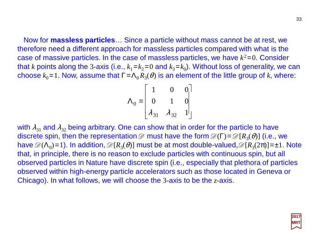
Now for massless particles … Since a particle without mass cannot be at rest, we therefore need a different approach for massless particles compared with what is the case of massive particles. In the case of massless particles, we have k2=0. Consider that k points along the 3-axis (i.e., k1=k2=0 and k3=k0). Without loss of generality, we can choose k0=1. Now, assume that Γ=Λ0R3(θ ) is an element of the little group of k, where:

33

2017MRT

=Λ1

010

001

3231

0

λλ

with λ31 and λ32 being arbitrary. One can show that in order for the particle to have discrete spin, then the representation D must have the form D(Γ)= D[R3(θ)] (i.e., we have D(Λ0)=1). In addition, D[R3(θ)] must be at most double-valued, D[R3(2π)] =±1. Note that, in principle, there is no reason to exclude particles with continuous spin, but all observed particles in Nature have discrete spin (i.e., especially that plethora of particles observed within high-energy particle accelerators such as those located in Geneva or Chicago). In what follows, we will choose the 3-axis to be the z-axis.

The irreducible representations of Rz(θ ) are trivial… Since Rz(θ ) belongs to an Abelian group, Schur’s lemma implies that the representations must be one-dimensional. This means that σ can take on only one value. Therefore, the numbers Dσ ′σ (Γ) are given by Dσ ′σ (Γ)=δσσ ′ dσ (θ ) where dσ (θ )=exp(−i σθ ). Since D[Rz(2π)] =±1, it implies that σ is an integer or a half-integer. This in turn means that the unitary operator can be written as U[Rz(θ )] =exp(−iθSz). In the case of massless particles, σ is the spin along the z-axis and is called the helicity. There is only one value for σ , which means that the helicity is (relativistically) invariant for massless particles. In general, if parity is included, then massless particles with spin s have only two independent helicity states ±σ (N.B., if σ =0, there is only one helicity state). No other states are allowed. This result is a property of massless particles and one of the consequences of Wigner’s method. For example, photons have spin 1, but only two helicity states ±1 are allowed. The absence of the helicity state 0 is due to the transverse nature of the field, which in turn is due to the absence of a photon rest mass. Other examples are gluons and possibly gravitons, which also exist in two helicity states only. Gluons, like photons, have helicity states ±1, whereas gravitons would have helicity states ±2. Finally, neutrinos are particles with spin ½ and have historically been assumed to be massless. In fact, there are now strong evidence that neutrinos are massive particles, albeit there masses are indeed extremely small (N.B., recently this has been shown to be the case but it has also given rise to conformity issues: http://phys.org/news/2017-02-precise-reactor-antineutrino-spectrum-reveals.html). Nevertheless, if we assume neutrinos to be massless, then neutrinos would have only helicity −½, whereas antineutrinos would always have helicity ½.

34

2017MRT

Let us discuss the transformation properties of the massless states |k,σ ⟩. Acting by a unitary operator of an element in the little group of k on these states gives:

35

2017MRT

What about Λ( p)? Here Λ( p) is the Lorentz transformation which transforms k to p. We choose k0 =1 and Λ( p)=Rz××××p(Θ)L( pz) where L( pz) is a pure boost along the z-axis such that L(pz)k=pz, pz

0=p0, pz1=pz

2=0, and pz3=p0 and Rz××××p(Θ) is a rotation Θ around the axis

z××××p. Since, by definition:

σσ θσ ,e,)( )( kkU i Γ−=Γ

we have:

σσ ,)]([, kpUp Λ=

where θ (Λ,p) is the angle of the rotation around the z-axis in:

σσ θσ ,e,)( ),( ppU pi Λ=Λ Λ−

σσδδσσ ′=′ )(,, 0 kp −−−−pkp

Here we have used the normalization:

where:

)()(),( 1 pHpHp ΛΛ=ΛΓ −

which becomes:

)()()( zpLRpH Θ= pz××××

)],([),( pRp zt ΛΛ=ΛΓ θ

The dynamical behavior of a single particle (i.e., a mass point with no real dimension as is the case in classical mechanics) can be inferred from Lagrange’s equation of motion:

36

2017MRT

Second Quantization

with the generalized coordinate qi and the generalized velocity dqi /dt ≡qi . This equation above is derivable from Hamilton’s variational principle which minimizes the action:

0=∂∂−

∂∂

ii q

L

q

L

td

d&

0),(2

1

== ∫t

tii qqLtdS &δδ

The Lagrangian L≡L(qi ,qi ) (N.B., we assume here no explicit dependence on the time t) is given by the difference between the kinetic energy T and the potential energy V:

VTL −=and the variation principle above is to be taken over an arbitrary path qi (t) such that δqi

vanishes at t1 and t2. The Hamiltonian of the system is:

LqpHi

ii −=∑ &

where the canonical momentum pi (i.e., the canonical conjugate to the coordinate qi ), is given by:

ii q

Lp

&∂∂≡

⋅

⋅

In the transition from the Lagrangian to the Hamiltonian system, we have exchanged independent variables from qi , qi to qi , pi . To prove that H(qi ,pi) is not a function of qi, we can make the following variation (N.B., recall the implied sum over coordinate index i):

),()(

)],([),(

iiii

iiiiii

qqLqp

qqLqppqH

&&

&&

δδδδ

−=−=

⋅⋅⋅⋅ ⋅⋅⋅⋅

by using the chain rule for that last step. Now, by equating the coefficients of the variation, we can make the following identification:

⋅⋅⋅⋅

ii

ii q

Hp

p

Hq

δδ

δδ =−= && and

where we have used Lagrange’s equation of motion (i.e., d(δ L/δ qi )/dt−δ L/δ qi =0).

2017MRT

37

ii

ii

ii

ii

iiii

qq

Lpq

qq

Lq

q

LqpqpH

δδδδ

δδδδ

δδδδδ

−=

−−+=

&

&&

&&

and following through with the rules of variations (very similar to differentiation), we get:

ii

ii q

Hq

p

HpH

δδδ

δδδδ +=

where we have used the above definition of pi ≡δ L/δ qi to eliminate the dependence of the Hamiltonian on qi so as to finally obtain: ⋅⋅⋅⋅

⋅⋅⋅⋅

In the Hamiltonian formalism, we can also calculate the time variation of any field F in terms of the Hamiltonian:

iiii

ii

ii

q

H

p

F

p

H

q

F

t

F

pp

Fq

q

F

t

FF

δδ

δδ

δδ

δδ

δδ

δδ

−+∂∂=

++∂∂= &&&

If we define the Poisson bracket as:

∑

∂∂

∂∂−

∂∂

∂∂=

i iiii p

B

q

A

q

B

p

ABA PB},{

then we can write the time variation of the field F as:

2017MRT

PB},{ FHt

FF +

∂∂=&

At this point, we have derived the Newtonian equations of motion by minimizing the action (i.e., the classical Newtonian path taken by the particle is the one in which the action is a minimum, δS=0), reproducing classical results. This is not new. However, we will now make the transition to the quantum theory, which treats the action as the fundamental object, incorporating both allowed and forbidden paths. The Newtonian equations of motion then specify the most likely path, but certainly not the only path. In the subatomic realm, in fact, the classically forbidden paths may dominate over the classical one.

38

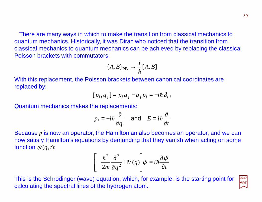
There are many ways in which to make the transition from classical mechanics to quantum mechanics. Historically, it was Dirac who noticed that the transition from classical mechanics to quantum mechanics can be achieved by replacing the classical Poisson brackets with commutators:

With this replacement, the Poisson brackets between canonical coordinates are replaced by:

],[},{ PB BAi

BAh

→

Quantum mechanics makes the replacements:

2017MRT

jiijjiji ipqqpqp δh−=−=],[

Because p is now an operator, the Hamiltonian also becomes an operator, and we can now satisfy Hamilton’s equations by demanding that they vanish when acting on some function ψ (q, t):

tiE

qip

ii ∂

∂=∂∂−= hh and

tiqV

qm ∂∂=

+

∂∂− ψψ h

h)(

2 2

22

This is the Schrödinger (wave) equation, which, for example, is the starting point for calculating the spectral lines of the hydrogen atom.

39

The standard quantum mechanical process of treating the generalized position and momentum, qi and pi, respectively (e.g., in providing the transition from the Lagrangian to the Hamiltonian variables from qi, qi to qi, pi ), as quantized variables, formulated by the transition from classical to quantum mechanics achieved by replacing the classical Poisson brackets with commutators (i.e., with Dirac’s prescription { A,B} PB→ (i /h)[ A,B]), is called first quantization. The transition from quantum mechanics to quantum field theory arises when we make the transition from three degrees of freedom, described by x i (with i =1,2,3) to an infinite number of degrees of freedom, described by a field φ(x i)and then apply quantization relations directly onto the fields.

40

2017MRT

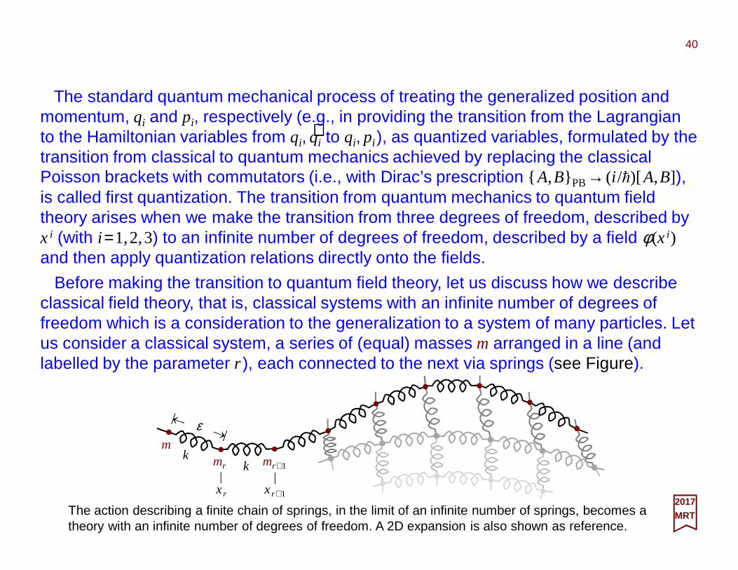
Before making the transition to quantum field theory, let us discuss how we describe classical field theory, that is, classical systems with an infinite number of degrees of freedom which is a consideration to the generalization to a system of many particles. Let us consider a classical system, a series of (equal) masses m arranged in a line (and labelled by the parameter r ), each connected to the next via springs (see Figure).

The action describing a finite chain of springs, in the limit of an infinite number of springs, becomes a theory with an infinite number of degrees of freedom. A 2D expansion is also shown as reference.

⋅⋅⋅⋅

k

ε

mr mr +1

xr xr +1

k

m

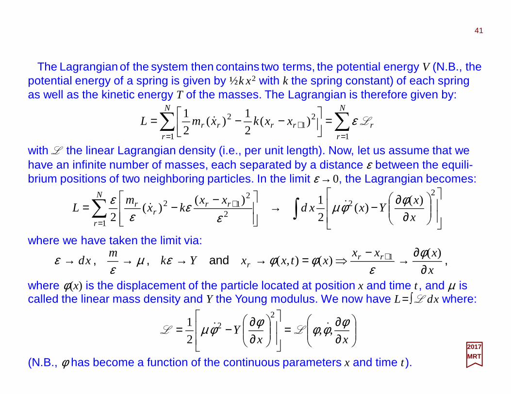
The Lagrangian of the system then contains two terms, the potential energy V (N.B., the potential energy of a spring is given by ½k x2 with k the spring constant) of each spring as well as the kinetic energy T of the masses. The Lagrangian is therefore given by:

with L the linear Lagrangian density (i.e., per unit length). Now, let us assume that we have an infinite number of masses, each separated by a distance ε between the equili-brium positions of two neighboring particles. In the limit ε →0, the Lagrangian becomes:

∑∑==

+ =

−−=N

rr

N

rrrrr xxkxmL

11

21

2 )(2

1)(

2

1Lε&

41

2017MRT

∫∑

∂∂−→

−−=

=

+2

2

12

212 )(

)(2

1)()(

2 x

xYxxd

xxkx

mL

N

r

rrr

r φφµε

εε

ε &&

where we have taken the limit via:

,and,,x

xxxxtxxYk

mxd rr

r ∂∂→−

⇒=→→→→ + )()(),( 1 φ

εφφεµ

εε

where φ(x) is the displacement of the particle located at position x and time t , and µ is called the linear mass density and Y the Young modulus. We now have L= ∫ L dx where:

∂∂=

∂∂−=

xxY

φφφφφµ ,,2

12

2 && LL

(N.B., φ has become a function of the continuous parameters x and time t ).

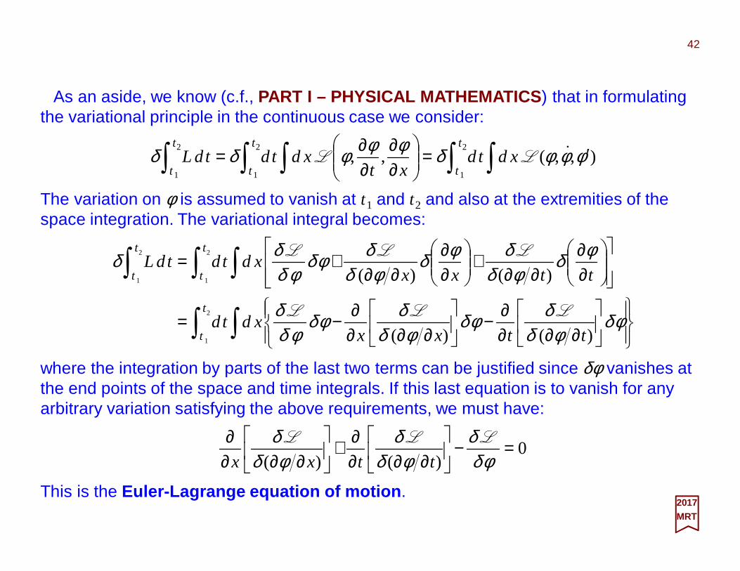
As an aside, we know (c.f., PART I – PHYSICAL MATHEMATICS ) that in formulating the variational principle in the continuous case we consider:

The variation on φ is assumed to vanish at t1 and t2 and also at the extremities of the space integration. The variational integral becomes:

42

2017MRT

∫ ∫∫ ∫∫ ′=

∂∂

∂∂=

2

1

2

1

2

1

),,(,,t

t

t

t

t

txdtd

xtxdtdtdL φφφδφφφδδ &LL

∫ ∫

∫ ∫∫

∂∂∂∂−

∂∂∂∂−=

∂∂

∂∂+

∂∂

∂∂+=

2

1

2

1

2

1

)()(

)()(

t

t

t

t

t

t

ttxxxdtd

ttxxxdtdtdL

φδφδ

δφδφδ

δφδφδ

δ

φδφδ

δφδφδ

δφδφδ

δδ

LLL

LLL

where the integration by parts of the last two terms can be justified since δφ vanishes at the end points of the space and time integrals. If this last equation is to vanish for any arbitrary variation satisfying the above requirements, we must have:

0)()(

=−

∂∂∂∂+

∂∂∂∂

φδδ

φδδ

φδδ LLL

ttxx

This is the Euler-Lagrange equation of motion .

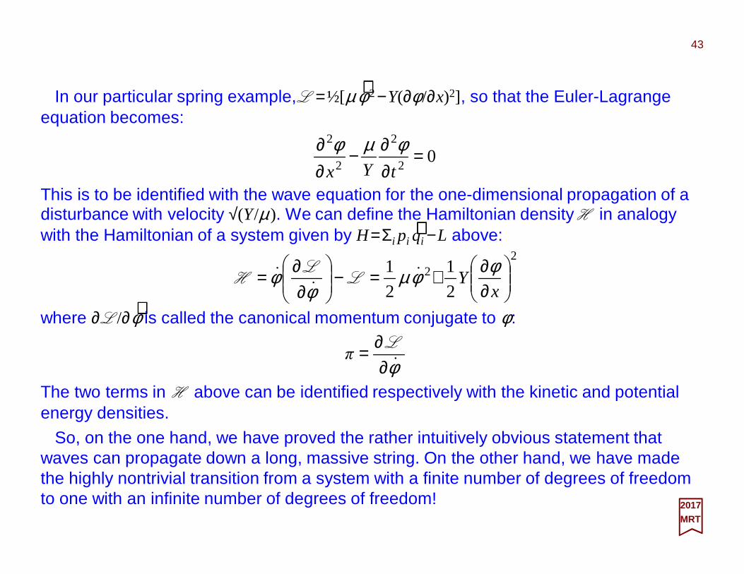
In our particular spring example, L =½[µ φ 2−Y(∂φ /∂x)2], so that the Euler-Lagrange equation becomes:

This is to be identified with the wave equation for the one-dimensional propagation of a disturbance with velocity √(Y/µ ). We can define the Hamiltonian density H in analogy with the Hamiltonian of a system given by H=Σi pi qi −L above:

43

2017MRT

02

2

2

2

=∂∂−

∂∂

tYx

φµφ

⋅⋅⋅⋅

where ∂ L /∂φ is called the canonical momentum conjugate to φ :

⋅⋅⋅⋅2

2

2

1

2

1

∂∂+=−

∂∂=

xY

φφµφ

φ &&

& LL

H

⋅⋅⋅⋅

φ&∂∂= L

π

The two terms in H above can be identified respectively with the kinetic and potential energy densities.

So, on the one hand, we have proved the rather intuitively obvious statement that waves can propagate down a long, massive string. On the other hand, we have made the highly nontrivial transition from a system with a finite number of degrees of freedom to one with an infinite number of degrees of freedom!

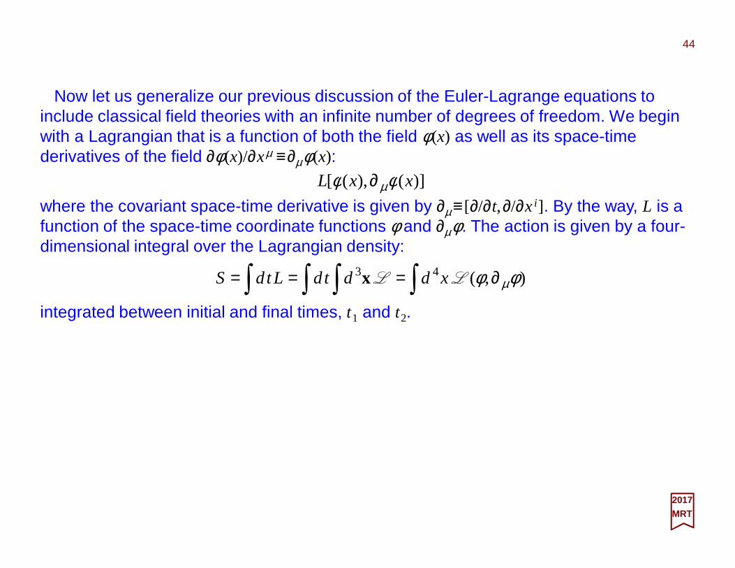
Now let us generalize our previous discussion of the Euler-Lagrange equations to include classical field theories with an infinite number of degrees of freedom. We begin with a Lagrangian that is a function of both the field φ(x) as well as its space-time derivatives of the field ∂φ(x)/∂xµ ≡∂µφ(x):

where the covariant space-time derivative is given by ∂µ ≡ [∂/∂t,∂/∂x i ]. By the way, L is a function of the space-time coordinate functions φ and ∂µφ. The action is given by a four-dimensional integral over the Lagrangian density:

)](),([ xxL φφ µ∂

44

2017MRT

∫∫ ∫∫ ∂=== ),(43 φφ µLL xddtdLtdS x

integrated between initial and final times, t1 and t2.

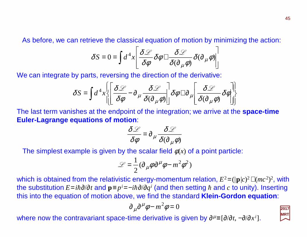
As before, we can retrieve the classical equation of motion by minimizing the action:

The simplest example is given by the scalar field φ(x) of a point particle:

)(2

1 22φφφ µµ m−∂∂=L

45

2017MRT

∫

∂

∂+== )(

)(0 4 φδ

φδδφδ

φδδδ µ

µ

LLxdS

We can integrate by parts, reversing the direction of the derivative:

∫

∂∂+

∂∂−= φδ

φδδφδ

φδδ

φδδδ

µµ

µµ )()(

4 LLLxdS

The last term vanishes at the endpoint of the integration; we arrive at the space-time Euler-Lagrange equations of motion :

)( φδδ

φδδ

µµ ∂

∂= LL

which is obtained from the relativistic energy-momentum relation, E2= (|p|c)2 + (mc2)2, with the substitution E= ih∂/∂t and p≡ pi =−ih∂/∂qi (and then setting h and c to unity). Inserting this into the equation of motion above, we find the standard Klein-Gordon equation :

02 =−∂∂ φφµµ m

where now the contravariant space-time derivative is given by ∂µ ≡ [∂/∂t, −∂/∂x i ].

As a slight aside, we will now consider including into the previous Klein-Gordon Lagrangian density L =−½(∂µ φ ∂ µφ−m2φ 2) (c.f., Second Quantization chapter) an interaction of the scalar field φ (i.e., φ ′=φ ) with a source density ρ :

46

2017MRT

Yukawa Potential

where the source density, which is, in general, a function of space-time coordinates, x (i.e., ρ =ρ(x)). The field equation now becomes:

φρ−=nInteractioL

22

2

∇−∂∂=∂∂=t

µµ�

where m is the mass (e.g., for a charged pion of mass µ =mc/h=140 MeV/c2 we have 1/µ=1.41×10−13 cm) and we have introduced the d’Alembertian operator :

ρφφ =− 2m�

Let us consider a static (i.e., time-independent) solution to φ −m2φ =ρ above where the source is assumed to be a point source at the origin, independent of time. We have:

�

)()( 322 xδφ Gm =−∇

where G, the numerical constant that characterizes the strength of the coupling of the field to the source, is analogous to the constant e in electrodynamics. Although the solu-tion of this last differential equation can also be guessed at immediately if you’ve had a freshman course in Mathematical Physics for Physics and Engineering students, for pedagogical reasons we will solve this equation using the Fourier transform method.

First, we define the transform φ (k) as follows:

47

2017MRT

where d3k and d3x, respectively, stand for volume elements in the three-dimensional k-space (i.e.,p=hk) and the coordinate x-space. Now, if we multiply both sides of (∇2 −m2)φ =Gδ 3(x) above by (2π)−3/2exp(−i k•x) and integrate with d3x, we obtain, after integrating by parts (N.B., assume that φ and ∇∇∇∇φ go to zero sufficiently rapidly at infinity):

∫∫ •−• == )(e)π2(

1)(

~)(

~e

)π2(

1)( 3

233

23xxkkkx xkxk φφφφ ii dd and

~

2322

)π2()(

~)(

Gm =−− kk φ

Thus the differential equation (∇2 −m2)φ =Gδ 3(x) above has been converted into an algebraic equation which can be solved:

∫ +−=

+−=

•

223

32223

e

)π2()(

1

)π2()(

~

md

G

m

G i

kkx

kk

xk

φφ and

so that, with r = |x|:

θk =∠(k ,x) and 2π= ∫0 to 2π dϕ . When the integration is done we get the Yukawa potential:

++−−≅−=

−K

22

21

π4

e

π4)( r

mrm

r

G

r

Gr

rm

φ

∫ ∫∞

∞− − +−=

1

1 22

cos23

3

e)(cosπ2

)π2()(

mdd

Gr

ri

kkk

kk

k

θθφ

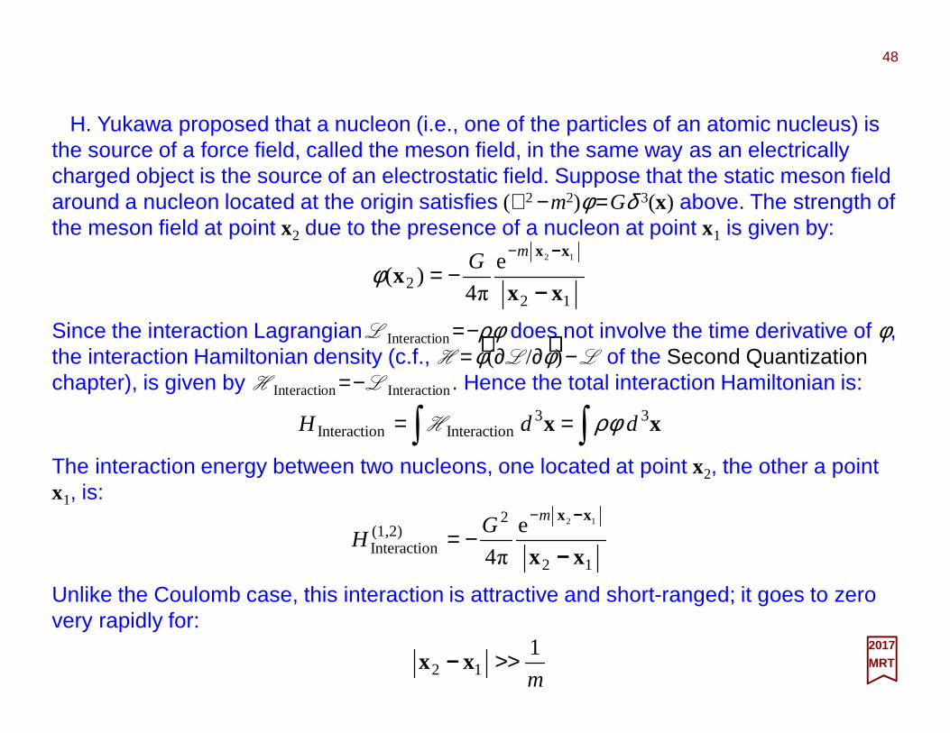
H. Yukawa proposed that a nucleon (i.e., one of the particles of an atomic nucleus) is the source of a force field, called the meson field, in the same way as an electrically charged object is the source of an electrostatic field. Suppose that the static meson field around a nucleon located at the origin satisfies (∇2 −m2)φ =Gδ 3(x) above. The strength of the meson field at point x2 due to the presence of a nucleon at point x1 is given by:

48

2017MRT

Since the interaction Lagrangian L Interaction=−ρφ does not involve the time derivative of φ, the interaction Hamiltonian density (c.f., H =φ(∂ L /∂φ)− L of the Second Quantizationchapter), is given by H Interaction=− L Interaction. Hence the total interaction Hamiltonian is:

122

12e

π4)(

xxx

xx

−−−−

−−−−mG −

−=φ

⋅⋅⋅⋅ ⋅⋅⋅⋅

∫∫ == xx 33nInteractionInteractio ddH φρH

The interaction energy between two nucleons, one located at point x2, the other a point x1, is:

12

2(1,2)

nInteractio

12e

π4 xx

xx

−−−−

−−−−mGH

−

−=

Unlike the Coulomb case, this interaction is attractive and short-ranged; it goes to zero very rapidly for:

m

112 >>xx −−−−

We have seen that by postulating the existence of a field obeying (∇2 −m2)φ =Gδ 3(x)above, we can quantitatively understand the short-ranged force between two nucleons. The mass of a quantum associated with the field was originally estimated by Yukawa to be about 200 times the electron mass. This estimate is not too far from the mass of the observed pion (i.e., mπ ≅ 270me or about 270 times the electron mass) discovered by C. F. Powell and his coworkers in 1947.

49

2017MRT

To represent the interaction of the pion field with the nucleon in a more realistic way, we must make a few more modifications. First, we must take into account the spin of the nucleus and the intrinsic odd parity of the pion. Second, we must note that the pions observed in nature have three charge states (π +,π0,π −). These considerations naturally lead us to a discussion of a complex field…

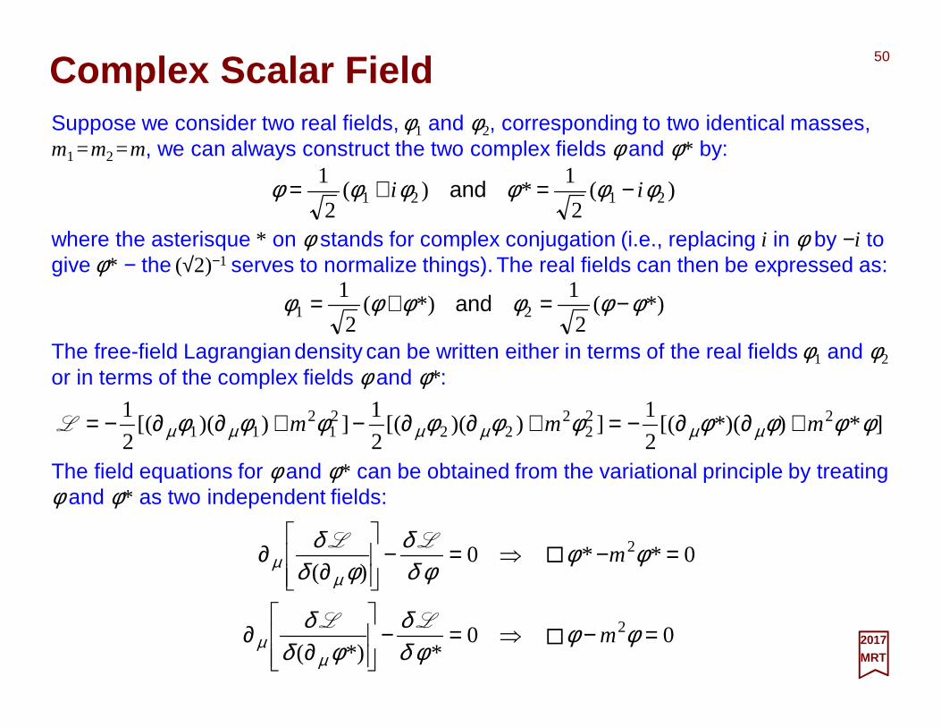
Suppose we consider two real fields, φ1 and φ2, corresponding to two identical masses, m1=m2=m, we can always construct the two complex fields φ and φ* by:

50

2017MRT

Complex Scalar Field

The free-field Lagrangian density can be written either in terms of the real fields φ1 and φ2

or in terms of the complex fields φ and φ*:

]*)*)([(2

1]))([(

2

1]))([(

2

1 222

222

21

211 φφφφφφφφφφ µµµµµµ mmm +∂∂−=+∂∂−+∂∂−=L

)(2

1*)(

2

12121 φφφφφφ ii −=+= and

where the asterisque * on φ stands for complex conjugation (i.e., replacing i in φ by −i to give φ* − the (√2)−1 serves to normalize things). The real fields can then be expressed as:

*)(2

1*)(

2

121 φφφφφφ −=+= and

The field equations for φ and φ* can be obtained from the variational principle by treating φ and φ* as two independent fields:

00**)(

0**0)(

2

2

=−⇒=−

∂∂

=−⇒=−

∂∂

φφφδ

δφδ

δ

φφφδ

δφδ

δ

µµ

µµ

m

m

LL

LL�

�

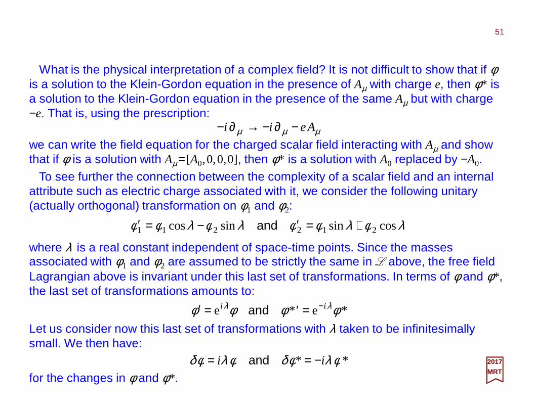
What is the physical interpretation of a complex field? It is not difficult to show that if φis a solution to the Klein-Gordon equation in the presence of Aµ with charge e, then φ* is a solution to the Klein-Gordon equation in the presence of the same Aµ but with charge −e. That is, using the prescription:

51

2017MRT

µµµ Aeii −∂−→∂−we can write the field equation for the charged scalar field interacting with Aµ and show that if φ is a solution with Aµ = [A0,0,0,0], then φ* is a solution with A0 replaced by −A0.

To see further the connection between the complexity of a scalar field and an internal attribute such as electric charge associated with it, we consider the following unitary (actually orthogonal) transformation on φ1 and φ2:

λφλφφλφλφφ cossinsincos 212211 +=′−=′ and

where λ is a real constant independent of space-time points. Since the masses associated with φ1 and φ2 are assumed to be strictly the same in L above, the free field Lagrangian above is invariant under this last set of transformations. In terms of φ and φ*, the last set of transformations amounts to:

*e*e φφφφ λλ ii −=′=′ and

Let us consider now this last set of transformations with λ taken to be infinitesimally small. We then have:

for the changes in φ and φ*.

** φλφδφλφδ ii −== and

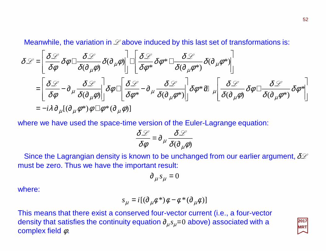
Meanwhile, the variation in L above induced by this last set of transformations is:

52

2017MRT

where we have used the space-time version of the Euler-Lagrange equation:

)( φδδ

φδδ

µµ ∂

∂= LL

Since the Lagrangian density is known to be unchanged from our earlier argument, δ Lmust be zero. Thus we have the important result:

0=∂ µµ s

where: )](**)[( φφφφ µµµ ∂−∂= is

This means that there exist a conserved four-vector current (i.e., a four-vector density that satisfies the continuity equation ∂µ sµ =0 above) associated with a complex field φ.

)](**)[(

**)()(

**)(*)(

*)(*)(

**

)()(

φφφφλ

φδφδ

δφδφδ

δφδφδ

δφδ

δφδφδ

δφδ

δ

φδφδ

δφδφδ

δφδφδ

δφδφδ

δδ

µµµ

µµµ

µµ

µµ

µµ

µµ

∂+∂∂−=

∂+

∂+∂

∂∂−+

∂∂−=

∂

∂++

∂

∂+=

i

LLLLLL

LLLLL

Under the substitution φ ↔ φ*, sµ changes its sign. This suggests that sµ is to be interpreted as the charge-current density up to a constant, and that if φ is a field corresponding to a particle with charge e, then φ* is a field corresponding to a particle with charge −e, in agreement with the interpretation suggested earlier in this chapter. It is a remarkable feature of relativistic field theory that it can readily accommodate a pair of particles with the same mass but opposite charges. In the formalism, however, there is nothing that compels up to replace sµ to the charge-current density that appears in electrodynamics. In fact, our formalism can accommodate any conserved internal attribute associated with a complex field.

53

2017MRT

Let us get back to pions. In order to describe the three charge states (π +,π 0,π −)observed in nature (via experiments in very expensive laboratories), we ignore the mass difference between the π ± and the π0 (i.e., about 5 MeV out of 140 MeV) and start with:

where the orthogonal linear combinations of φ1 and φ2 given by φ =(√2)−1(φ1+ iφ2) and φ* =(√2)−1(φ1− iφ2) correspond to the charged pions, and φ3 corresponds to the neutral pion. This suggests that not only φ1 and φ2 but also all three φ k (k =1,2,3) are mixed with one another. This is essentially the starting point of the isospin formalism, a subject which we shall discuss at length in PART VIII – THE STANDARD MODEL .

+∂∂−= ∑

=kk

kkk m φφφφ µµ

23

1

)()(2

1L

To sum up, the strict mass degeneracy of φ1 and φ2 implies the invariance of L under φ1′=φ1cosλ +φ2sinλ and φ2′=φ1sinλ −φ2cosλ as well as φ ′=exp(iλ)φ and φ* ′=exp(−iλ)φ*which in turn gives the conservation laws of electric charge, or some similar internal attribute, associated with the complex fields φ and φ*. The connection between invariance under a certain transformation and an associated conservation law is well known in both classical and quantum mechanics (e.g., the connection between rotational invariance – i.e., the isotropy of space – and angular momentum conservation). But here we see that the conservation law of a non-geometrical attribute such as electric charge can also be formulated in terms of invariance under the set of transformations φ ′=exp(iλ)φ and φ* ′=exp(−iλ)φ* which is called, after W. Pauli, the gauge transformation of the first kind (N.B., ‘gauge’ it is actually pronounced as ‘gáge’).

54

2017MRT

Perhaps the real significance of what we have accomplished can be appreciated only by considering an example in which the conservation of an internal attribute is approximate. In field theory, neutral K mesons created in high-energy collisions must be described by complex fields even though they are electrically neutral. This is because K 0

and its antiparticle K 0 carry internal attributes called hypercharge, denoted by Y; Y=+1for K 0 with which we may associate a complex field φ, and Y=−1 for K 0 with which we may associate φ*. Hypercharge conservation (which is equivalent to conservation of strangeness, introduced by M. Gell-Mann and K. Nishijima in 1953) is a very useful conservation law, but it is broken by a class of interactions about 1012 times weaker than the kind of interactions responsible for the production of K 0 and K 0 with definite hypercharges. As a result, the particle states known as K 1 and K 2 which essentially correspond to our φ1 and φ2 turn out to have a very small but measurable mass difference (i.e., ~10−11 MeV/c2). Thanks to the nonconservation of hypercharge we have a realistic example that illustrates the connection between the nonconservation of an internal attribute and a removal of the mass degeneracy.

55

2017MRT

−−

−

2017MRT

One of the achievement of this formulation is that we can use symmetries of the action to derive conservation principles. For example, in classical mechanics, if the Hamiltonian is time independent, then energy is conserved. Likewise, if the Hamiltonian is translation invariant in three dimensions, then momentum is conserved. Finally, if we have rotational independence, we also have angular momentum conservation.

Noether’s Theorem

The precise mathematical formulation of this correspondence is given by Noether’s theorem. In general, an action may be invariant under either an internal, isospin (i.e., a quantum number related to the strong interaction) symmetry transformation of the fields, or under some space-time (i.e., combined space and time continuum) symmetry.

56

∫

∫∫

∂∂=

∂

∂+

∂∂=

∂

∂+=

kk

kk

kk

kk

kk

xd

xdxdS

φδφδ

δ

φδφδ

δφδφδ

δφδφδ

δφδφδ

δδ

µµ

µµµ

µµµ

L

LLLL

4

44 )()(

where we have used the Euler-Lagrange equation of motion and have converted the variation of the action into the integral of a total derivative. This defines the current J µ k:

k

l

lkJεδφδ

φδδ

µ

µ

∂= L

We will first discuss the isospin symmetry, where the fields φ k (k =1,2,3) vary accor-ding to some small parameter δε k. The action varies as:

2017MRT

If the action is invariant under this transformation, then we have established that the current is conserved:

From this conserved current, we can also establish a conserved charge, given by the integral over the fourth component of the current:

57

0=∂ µµ kJ

∫≡ x30 dJQ kk

Now, let us investigate the second case, when the action is invariant under the space-time symmetry of the Lorentz and Poincaré groups. Lorentz symmetry implies that we can combine familiar three-vectors, such as momentum and space, into four-vectors. We introduce the space-time coordinate xµ as follows:

In summary, the (isospin) symmetry of the action implies the conservation of a current Jµ

k, which in turn implies a conservation principle: Symmetry→Current Conservation→Conservation Principle.

],[],[ 0 xtxxx i =≡µ

where the time coordinate is defined as x0= t (i.e., with the velocity of light c≡1). Similarly, the momentum three-vector p can be combined with energy to form the four-

vector: ],[],[ 0 pEppp i =≡µ

As usual, Greek symbols represent four-vectors and Latin indices space coordinates.

2017MRT

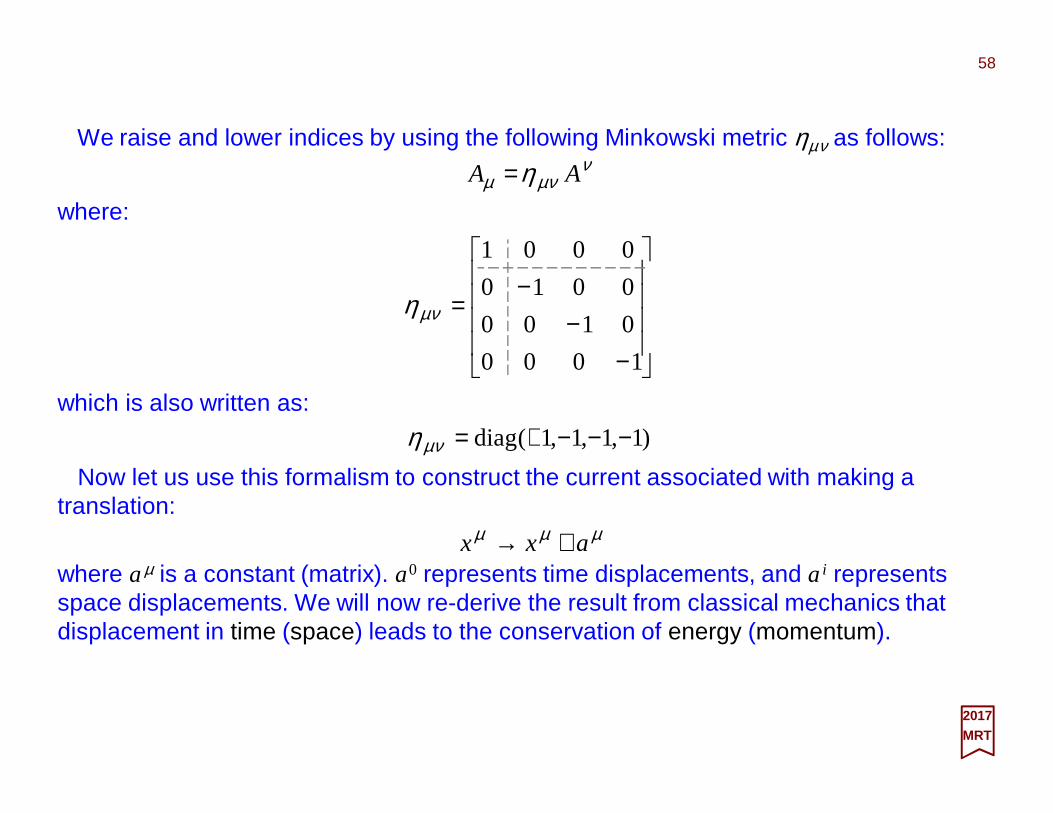
We raise and lower indices by using the following Minkowski metric ηµν as follows:

where:

58

ννµµ η AA =

−−

−=

1000

0100

0010

0001

νµη

Now let us use this formalism to construct the current associated with making a translation:

µµµ axx +→where aµ is a constant (matrix). a0 represents time displacements, and ai represents space displacements. We will now re-derive the result from classical mechanics that displacement in time (space) leads to the conservation of energy (momentum).

which is also written as:

)1,1,1,1(diag −−−+=νµη

2017MRT

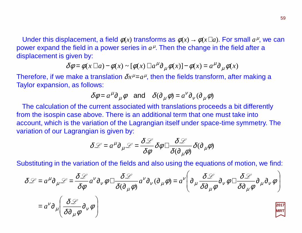
Under this displacement, a field φ (x) transforms as φ (x)→φ (x+a). For small aµ, we can power expand the field in a power series in aµ. Then the change in the field after a displacement is given by:

Therefore, if we make a translation δ xµ =aµ, then the fields transform, after making a Taylor expansion, as follows:

59

)()()]()([~)()( xaxxaxxax φφφφφφφδ µµ

µµ ∂=−∂+−+=

)()( φφδφφδ µνν

µµµ ∂∂=∂∂= aa and

The calculation of the current associated with translations proceeds a bit differently from the isospin case above. There is an additional term that one must take into account, which is the variation of the Lagrangian itself under space-time symmetry. The variation of our Lagrangian is given by:

)()(

φδφδ

δφδφδ

δδ µµ

µµ ∂

∂+=∂= LL

LL a

Substituting in the variation of the fields and also using the equations of motion, we find:

∂

∂∂=

∂∂

∂+∂

∂∂=∂∂

∂+∂=∂=

φφδ

δ

φφδ

δφφδ

δφφδ

δφφδ

δδ

νµ

µν

νµµ

νµ

µν

µνν

µν

νµ

µ

L

LLLLLL

a

aaaa )()(

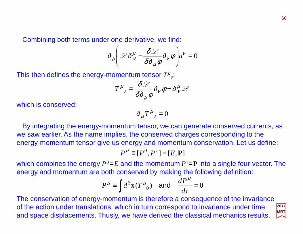
2017MRT

Combining both terms under one derivative, we find:

This then defines the energy-momentum tensor Tµν:

60

0=

∂

∂−∂ ν

νµ

µνµ φ

φδδδ aL

L

LL µ

ννµ

µν δφ

φδδ −∂∂

=T

which is conserved: 0=∂ µ

νµ T

By integrating the energy-momentum tensor, we can generate conserved currents, as we saw earlier. As the name implies, the conserved charges corresponding to the energy-momentum tensor give us energy and momentum conservation. Let us define:

],[],[ 0 PEPPP i =≡µ

which combines the energy P0=E and the momentum P i =P into a single four-vector. The energy and momentum are both conserved by making the following definition:

0)( 03 =≡ ∫ td

PdTdP

µµµ andx

The conservation of energy-momentum is therefore a consequence of the invariance of the action under translations, which in turn correspond to invariance under time and space displacements. Thusly, we have derived the classical mechanics results.

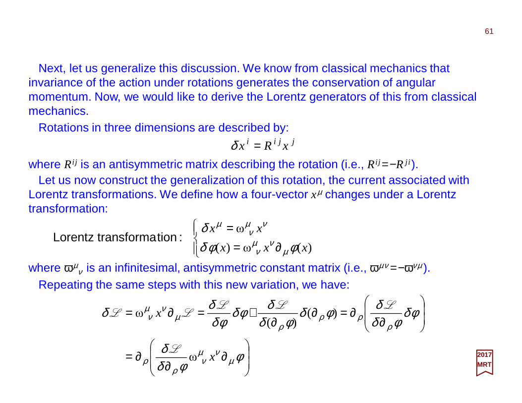
Next, let us generalize this discussion. We know from classical mechanics that invariance of the action under rotations generates the conservation of angular momentum. Now, we would like to derive the Lorentz generators of this from classical mechanics.

Rotations in three dimensions are described by: jjii xRx =δ

61

2017MRT

where Ri j is an antisymmetric matrix describing the rotation (i.e., Ri j =−R j i ). Let us now construct the generalization of this rotation, the current associated with

Lorentz transformations. We define how a four-vector xµ changes under a Lorentz transformation:

∂==

)(ω)(

ω

xxx

xx

φφδδ

µνµ

ν

νµν

µ:tiontransforma Lorentz

where ωµν is an infinitesimal, antisymmetric constant matrix (i.e., ωµν =−ωνµ ).

∂

∂∂=

∂∂=∂

∂+=∂=

φφδ

δ

φδφδ

δφδφδ

δφδφδ

δδ

µνµ

νρ

ρ

ρρρ

ρµ

νµν

x

x

ω

)()(

ω

L

LLLLL

Repeating the same steps with this new variation, we have:

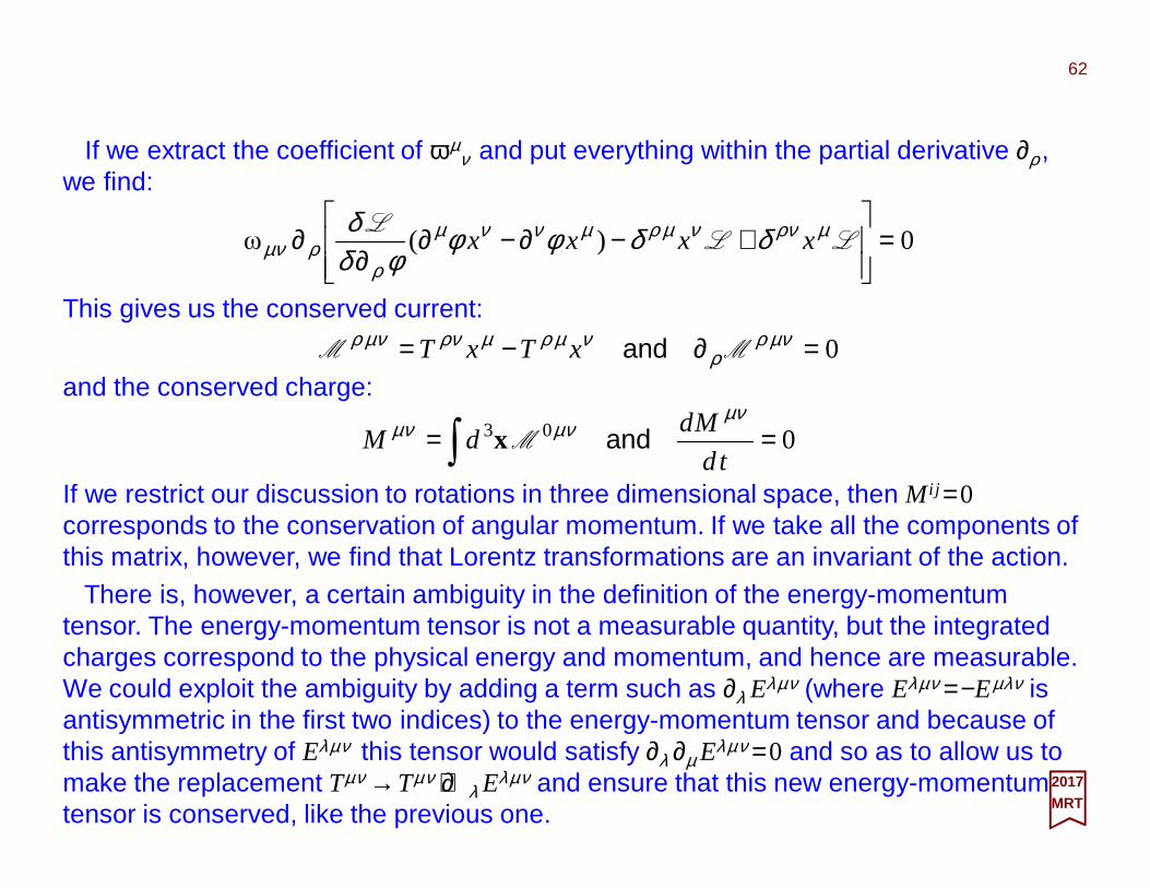
If we extract the coefficient of ωµν and put everything within the partial derivative ∂ρ ,

we find:

This gives us the conserved current:

0=∂−= νµρρ

νµρµνρνµρMM andxTxT

62

2017MRT

0)(ω =

+−∂−∂

∂∂ LL

L µνρνµρµννµ

ρρνµ δδφφ

φδδ

xxxx

and the conserved charge:

003 == ∫ td

MddM

νµνµνµ andMx

If we restrict our discussion to rotations in three dimensional space, then M i j =0 corresponds to the conservation of angular momentum. If we take all the components of this matrix, however, we find that Lorentz transformations are an invariant of the action.

There is, however, a certain ambiguity in the definition of the energy-momentum tensor. The energy-momentum tensor is not a measurable quantity, but the integrated charges correspond to the physical energy and momentum, and hence are measurable. We could exploit the ambiguity by adding a term such as ∂λ Eλµν (where Eλµν =−Eµλν is antisymmetric in the first two indices) to the energy-momentum tensor and because of this antisymmetry of Eλµν this tensor would satisfy ∂λ ∂µ Eλµν =0 and so as to allow us to make the replacement Tµν →Tµν +∂λ Eλµν and ensure that this new energy-momentum tensor is conserved, like the previous one.

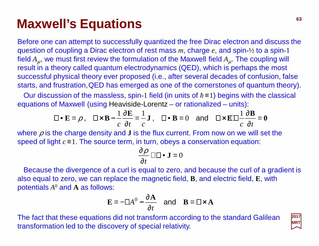
63

2017MRT

Before one can attempt to successfully quantized the free Dirac electron and discuss the question of coupling a Dirac electron of rest mass m, charge e, and spin-½ to a spin-1field Aµ, we must first review the formulation of the Maxwell field Aµ. The coupling will result in a theory called quantum electrodynamics (QED), which is perhaps the most successful physical theory ever proposed (i.e., after several decades of confusion, false starts, and frustration,QED has emerged as one of the cornerstones of quantum theory).

Maxwell’s Equations

Our discussion of the massless, spin-1 field (in units of h ≡1) begins with the classical equations of Maxwell (using Heaviside-Lorentz – or rationalized – units):

0B

EBJE

BE =∂∂=•=

∂∂=•

tcctc

10

11 ++++××××∇∇∇∇∇∇∇∇−−−−××××∇∇∇∇∇∇∇∇ and,,ρ

where ρ is the charge density and J is the flux current. From now on we will set the speed of light c≡1. The source term, in turn, obeys a conservation equation:

0=•+∂∂

J∇∇∇∇t

ρ

Because the divergence of a curl is equal to zero, and because the curl of a gradient is also equal to zero, we can replace the magnetic field, B, and electric field, E, with potentials A0 and A as follows:

ABA

E ××××∇∇∇∇−−−−∇∇∇∇ =∂∂−= and

tA0

The fact that these equations did not transform according to the standard Galilean transformation led to the discovery of special relativity.

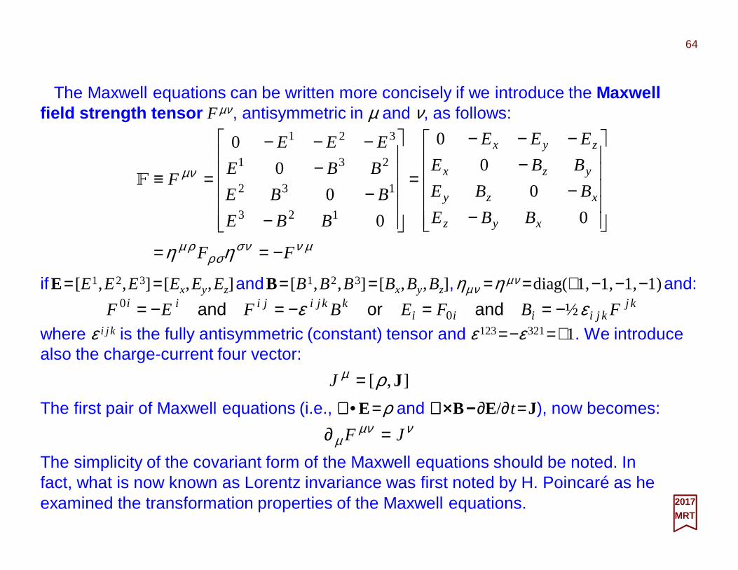
64

2017MRT

The Maxwell equations can be written more concisely if we introduce the Maxwell field strength tensor Fµν, antisymmetric in µ and ν, as follows:

µννσσρ

ρµ

νµ

ηη FF

BBE

BBE

BBE

EEE

BBE

BBE

BBE

EEE

F

xyz

xzy

yzx

zyx

−==

−−

−−−−

=

−−

−−−−

=≡

0

0

0

0

0

0

0

0

123

132

231

321

�

ifE= [E1,E2,E3] = [Ex,Ey,Ez] andB= [B1,B2,B3] = [Bx,By,Bz],ηµν =η µν =diag(+1,−1,−1,−1)and: kj

kjiiiikkjijiii FBFEBFEF εε ½0

0 −==−=−= andorandwhere ε i j k is the fully antisymmetric (constant) tensor and ε 123=−ε 321=+1. We introduce also the charge-current four vector:

],[ Jρµ =J

The first pair of Maxwell equations (i.e., ∇∇∇∇•E=ρ and ∇∇∇∇××××B −−−−∂E/∂t=J), now becomes: ννµ

µ JF =∂The simplicity of the covariant form of the Maxwell equations should be noted. In fact, what is now known as Lorentz invariance was first noted by H. Poincaré as he examined the transformation properties of the Maxwell equations.

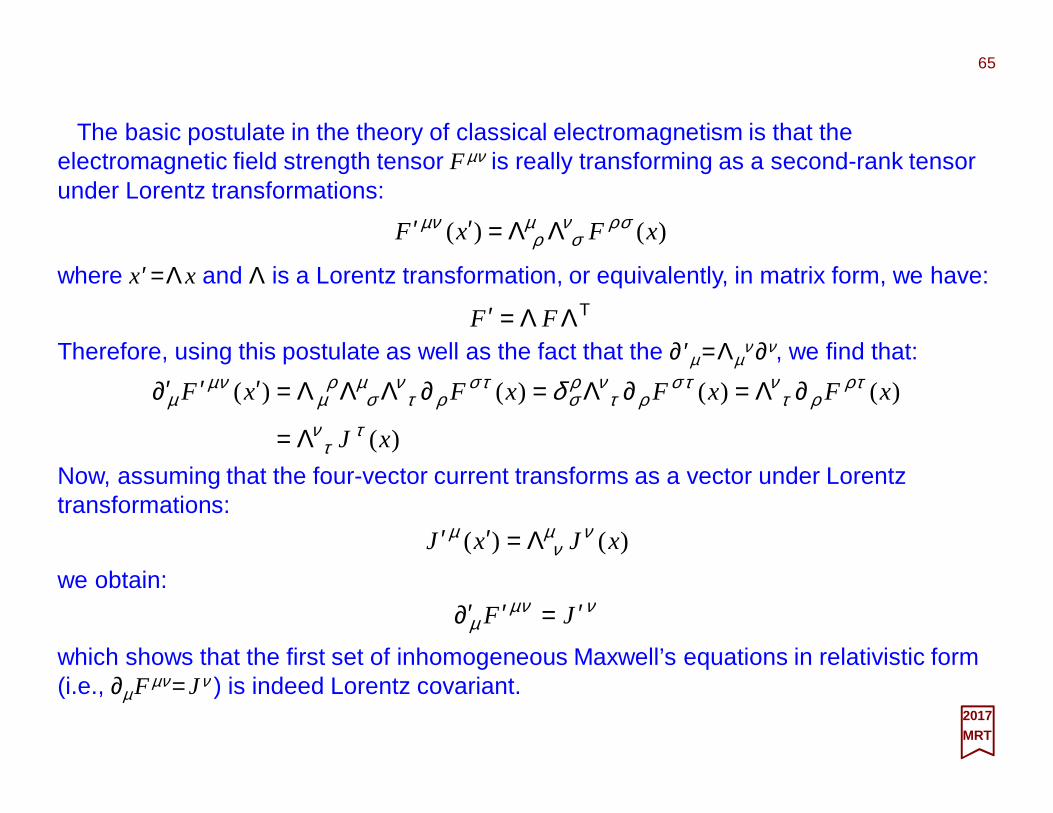
65

2017MRT

The basic postulate in the theory of classical electromagnetism is that the electromagnetic field strength tensor Fµν is really transforming as a second-rank tensor under Lorentz transformations:

)()( xFxF σρνσ

µρ

νµ ΛΛ=′′

where x′=Λx and Λ is a Lorentz transformation, or equivalently, in matrix form, we have:

Therefore, using this postulate as well as the fact that the ∂′µ =Λµν ∂ν, we find that:

)(

)()()()(

xJ

xFxFxFxF

τντ

τρρ

ντ

τσρ

ντ

ρσ

τσρ

ντ

µσ

ρµ

νµµ δ

Λ=

∂Λ=∂Λ=∂ΛΛΛ=′′∂′

Now, assuming that the four-vector current transforms as a vector under Lorentz transformations:

)()( xJxJ νµν

µ Λ=′′we obtain:

TΛΛ=′ FF

ννµµ JF ′=′∂′

which shows that the first set of inhomogeneous Maxwell’s equations in relativistic form (i.e., ∂µFµν = Jν ) is indeed Lorentz covariant.

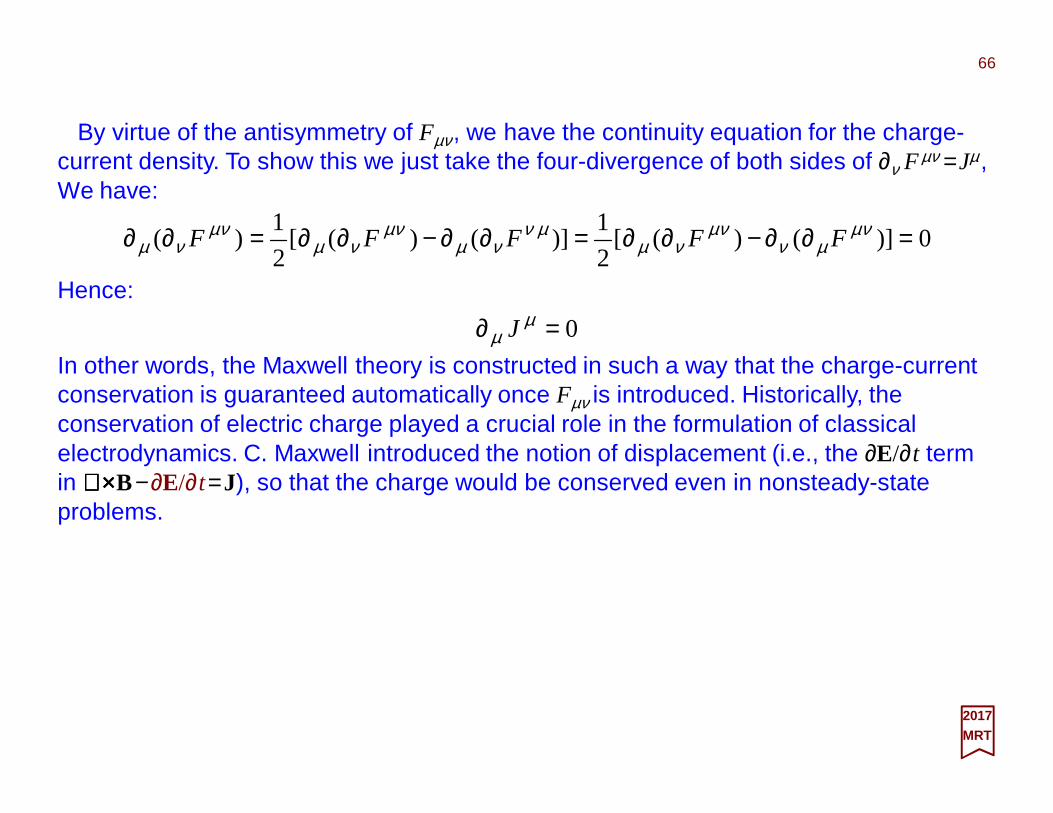
By virtue of the antisymmetry of Fµν, we have the continuity equation for the charge-current density. To show this we just take the four-divergence of both sides of ∂ν Fµν =Jµ, We have:

66

2017MRT

Hence:

0)]()([2

1)]()([

2

1)( =∂∂−∂∂=∂∂−∂∂=∂∂ νµ

µννµ

νµµν

νµνµ

νµνµ

νµ FFFFF

0=∂ µµ J

In other words, the Maxwell theory is constructed in such a way that the charge-current conservation is guaranteed automatically once Fµν is introduced. Historically, the conservation of electric charge played a crucial role in the formulation of classical electrodynamics. C. Maxwell introduced the notion of displacement (i.e., the ∂E/∂t term in ∇∇∇∇××××B−∂E/∂t=J), so that the charge would be conserved even in nonsteady-state problems.

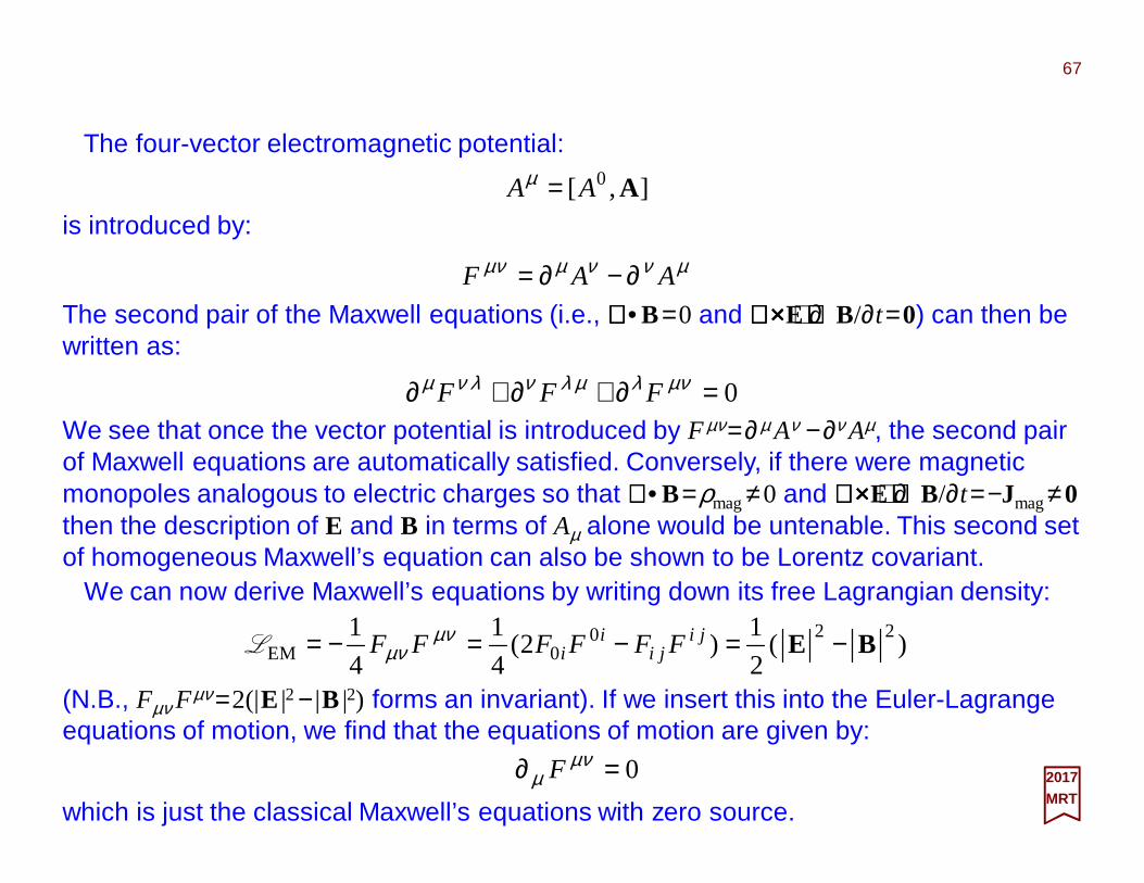
The four-vector electromagnetic potential:

67

2017MRT

0=∂+∂+∂ νµλµλνλνµ FFFWe see that once the vector potential is introduced by Fµν=∂ µ Aν −∂ν Aµ, the second pair of Maxwell equations are automatically satisfied. Conversely, if there were magnetic monopoles analogous to electric charges so that ∇∇∇∇•B=ρmag≠0 and ∇∇∇∇××××E ++++∂B/∂t=−Jmag≠0then the description of E and B in terms of Aµ alone would be untenable. This second set of homogeneous Maxwell’s equation can also be shown to be Lorentz covariant.

µννµνµ AAF ∂−∂=

],[ 0 AAA =µ

The second pair of the Maxwell equations (i.e., ∇∇∇∇•B=0 and ∇∇∇∇××××E ++++∂B/∂t=0) can then be written as:

is introduced by:

We can now derive Maxwell’s equations by writing down its free Lagrangian density:

(N.B., Fµν Fµν =2(|E |2 − |B |2) forms an invariant). If we insert this into the Euler-Lagrange equations of motion, we find that the equations of motion are given by:

)(2

1)2(

4

1

4

1 2200EM BE −=−=−= ji

jii

i FFFFFF νµνµL

0=∂ νµµ F

which is just the classical Maxwell’s equations with zero source.

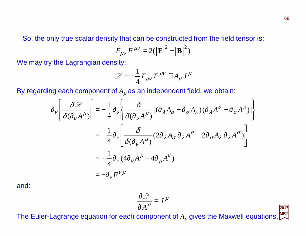
So, the only true scalar density that can be constructed from the field tensor is:

68

)(222

BE −=µνµν FF

2017MRT

We may try the Lagrangian density:

µµ

µνµν JAFF +−=

4

1L

By regarding each component of Aµ as an independent field, we obtain:

µνν

νµ

µνν

σλλσ

σλσλµ

νν

λσ

σλλσσλµ

ννµ

νν

δδ

δδ

δδ

F

AA

AAAAA

AAAAAA

−∂=

∂−∂∂−=

∂∂−∂∂

∂∂−=

∂−∂∂−∂∂

∂−=

∂∂

)44(4

1

)22()(4

1

)]()[()(4

1

)(

L

and:

The Euler-Lagrange equation for each component of Aµ gives the Maxwell equations.

µµ J

A=

∂∂ L

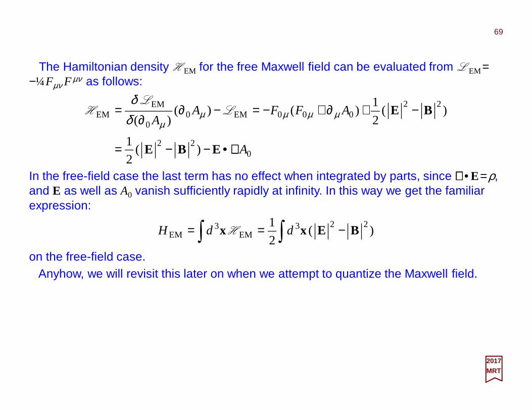
The Hamiltonian density HEM for the free Maxwell field can be evaluated from LEM=−¼Fµν Fµν as follows:

69

022

22000EM0

0

EMEM

)(2

1

)(2

1)()(

)(

A

AFFAA

∇∇∇∇•−−=

−+∂+−=−∂∂

=

EBE

BEµµµµµδ

δL

LH

2017MRT

In the free-field case the last term has no effect when integrated by parts, since ∇∇∇∇•E=ρ, and E as well as A0 vanish sufficiently rapidly at infinity. In this way we get the familiar expression:

∫∫ −== )(2

1 223EM

3EM BExx ddH H

on the free-field case. Anyhow, we will revisit this later on when we attempt to quantize the Maxwell field.

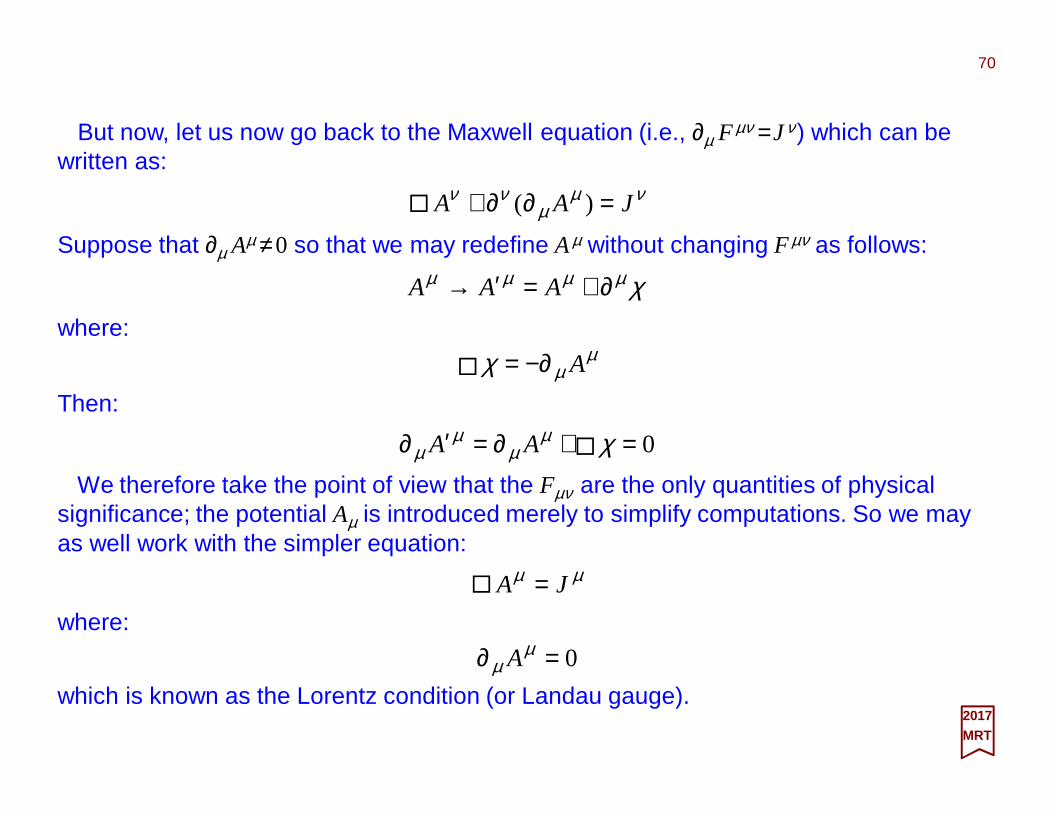
But now, let us now go back to the Maxwell equation (i.e., ∂µ Fµν =Jν) which can be written as:

70

2017MRT

Suppose that ∂µ Aµ ≠0 so that we may redefine Aµ without changing Fµν as follows:

νµµ

νν JAA =∂∂+ )(�

χµµµµ ∂+=′→ AAA

where: µ

µχ A−∂=�

Then:

0=+∂=′∂ χµµ

µµ AA �

We therefore take the point of view that the Fµν are the only quantities of physical significance; the potential Aµ is introduced merely to simplify computations. So we may as well work with the simpler equation:

µµ JA =�

where:

0=∂ µµ A

which is known as the Lorentz condition (or Landau gauge).

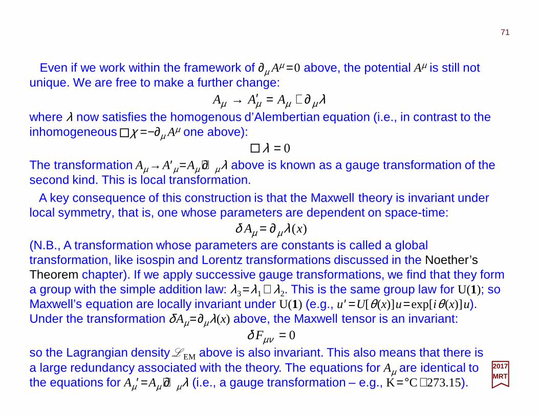
71

2017MRT

A key consequence of this construction is that the Maxwell theory is invariant under local symmetry, that is, one whose parameters are dependent on space-time:

)(xA λδ µµ ∂=(N.B., A transformation whose parameters are constants is called a global transformation, like isospin and Lorentz transformations discussed in the Noether’s Theorem chapter). If we apply successive gauge transformations, we find that they form a group with the simple addition law: λ3=λ1⊕λ2. This is the same group law for U(1); so Maxwell’s equation are locally invariant under U(1) (e.g., u′=U[θ (x)]u=exp[iθ (x)]u). Under the transformation δ Aµ=∂µ λ(x) above, the Maxwell tensor is an invariant:

0=νµδ Fso the Lagrangian density LEM above is also invariant. This also means that there is a large redundancy associated with the theory. The equations for Aµ are identical to the equations for Aµ′=Aµ +∂µλ (i.e., a gauge transformation – e.g., K =°C+273.15).

Even if we work within the framework of ∂µ Aµ =0 above, the potential Aµ is still not unique. We are free to make a further change:

λµµµµ ∂+=′→ AAAwhere λ now satisfies the homogenous d’Alembertian equation (i.e., in contrast to the inhomogeneous χ =−∂µ Aµ one above): �

0=λ�

The transformation Aµ →A′µ =Aµ +∂µ λ above is known as a gauge transformation of the second kind. This is local transformation.

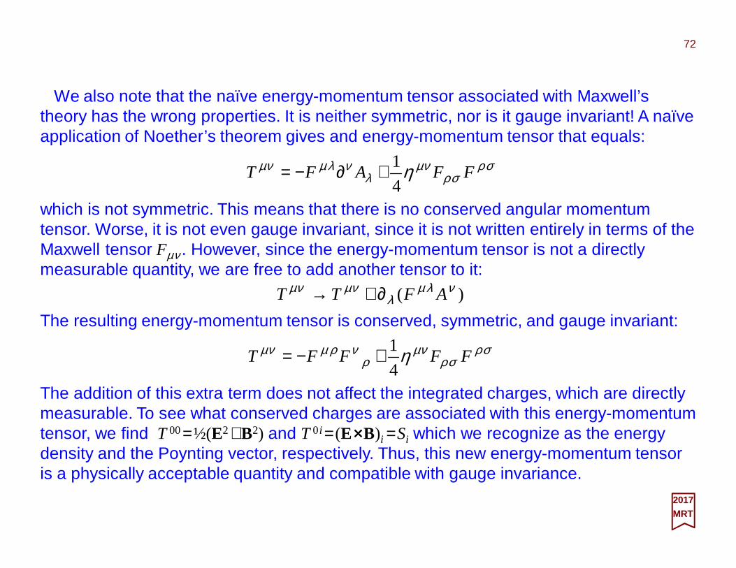
We also note that the naïve energy-momentum tensor associated with Maxwell’s theory has the wrong properties. It is neither symmetric, nor is it gauge invariant! A naïve application of Noether’s theorem gives and energy-momentum tensor that equals:

which is not symmetric. This means that there is no conserved angular momentum tensor. Worse, it is not even gauge invariant, since it is not written entirely in terms of the Maxwell tensor Fµν . However, since the energy-momentum tensor is not a directly measurable quantity, we are free to add another tensor to it:

σρσρ

νµλ

νλµνµ η FFAFT4

1+∂−=

72

2017MRT

)( νλµλ

νµνµ AFTT ∂+→The resulting energy-momentum tensor is conserved, symmetric, and gauge invariant:

σρσρ

νµνρ

ρµνµ η FFFFT4

1+−=

The addition of this extra term does not affect the integrated charges, which are directly measurable. To see what conserved charges are associated with this energy-momentum tensor, we find T00=½(E2+B2) and T0i = (E××××B)i =Si which we recognize as the energy density and the Poynting vector, respectively. Thus, this new energy-momentum tensor is a physically acceptable quantity and compatible with gauge invariance.

References / Study Guide

2017MRT

73

J.J. Sakurai, Advanced Quantum Mechanics , Addison-Wesley, 1967. University of California at Los Angeles

The tenth printing [mine] of this renowned textbook confirms its widely-regarded status as a classic. The book presents the major advances in the fundamentals of quantum physics from 1927 to the present day [1967]. No familiarity with relativistic quantummechanics of quantum field theory is presupposed, but the reader is assumed to be familiar with non-relativistic quantum mechanics, classical electrodynamics, and classical mechanics. The author’s clear presentation focuses on key concepts, giving attention toexperimental work in the field. M. Kaku, Quantum Field Theory – A Modern Introduction , Oxford University Press, 1993City College of the CUNY

The rise of quantum electrodynamics (QED) made possible a number of excellent textbooks on quantum field theory in the 1960s.However, the rise of quantum chromodynamics (QCD) and the Standard Model has made it urgent to have a fully modern textbook for the 1990s and beyond. Building on the foundation of QED, Quantum Field Theory: A Modern Introduction presents a clear andcomprehensive discussion of the gauge revolution and the theoretical and experimental evidence which makes the Standard Modelthe leading theory of subatomic phenomena. The book is divided into three parts: Part I, Fields and Renormalization, lays a solid foundation by presenting canonical quantization, Feynman rules and scattering matrices, and renormalization theory. Part II, Gauge Theory and the Standard Model, focuses on the Standard Model and discusses path integrals, gauge theory, spontaneous symmetrybreaking, the renormalization group, and BPHZ quantization. Part III, Non-perturbative Methods and Unification, discusses more advanced methods which now form an essential part of field theory, such as critical phenomena, lattice gauge theory, instantons,supersymmetry, quantum gravity, supergravity, and superstrings.T. Ohlsson, Relativistic Quantum Physics , Cambridge University Press, 2011. Royal Institute of Technology (KTH), SwedenQuantum physics and special relativity theory were two of the greatest breakthroughs in physics during the twentieth century andcontributed to paradigm shifts in physics. This book combines these two discoveries to provide a complete description of the fundamentals of relativistic quantum physics, guiding the reader effortlessly from relativistic quantum mechanics to basic quantum field theory. The book gives a thorough and detailed treatment of the subject, beginning with the classification of particles, the Klein-Gordon equation and the Dirac equation. It then moves on to the canonical quantization procedure of the Klein-Gordon, Dirac and electromagnetic fields. Classical Yang-Mills theory, the LSZ formalism, perturbation theory, elementary processes in QED are introduced, and regularization, renormalization and radiative corrections are explored. With exercises scattered through the text and problems at the end of most chapters, the book is ideal for advanced undergraduate and graduate students in theoretical physics.T. Banks, Modern Quantum Field Theory: A Concise Introduction , Cambridge University Press, 2008. University of California, Santa Cruz, and Rutgers UniversityThis comprehensive and progressive new text presents a variety of topics that are only briefly touched on in other books; this text provides a thorough introduction to the techniques of quantum field theory, which is the theoretical framework for constructing quantum mechanical models of field-like systems or, equivalently, of many-body systems. […] The Standard Model of particle physics is also discussed in detail. […] Ideal for graduate students in high-energy physics and condensed matter physics […]

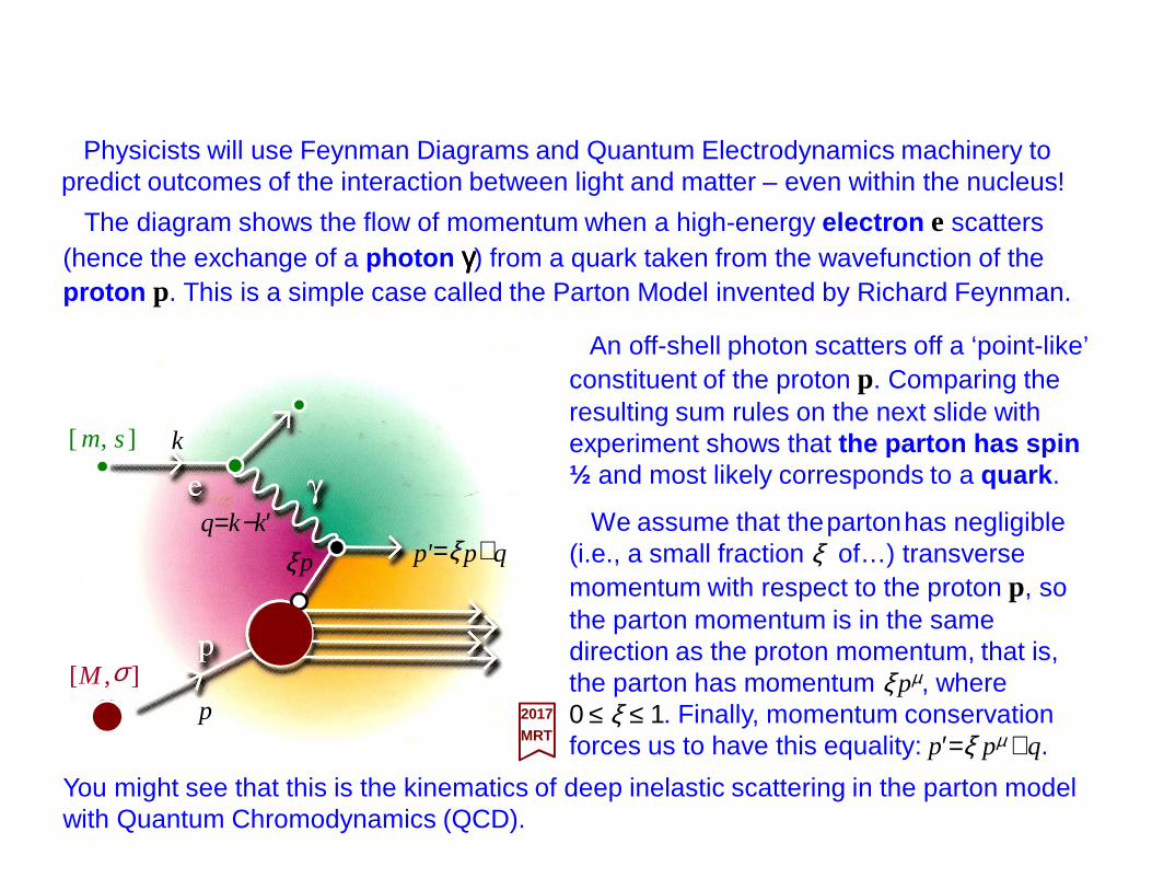
You might see that this is the kinematics of deep inelastic scattering in the parton model with Quantum Chromodynamics (QCD).

The diagram shows the flow of momentum when a high-energy electron e scatters (hence the exchange of a photon γγγγ) from a quark taken from the wavefunction of the proton p. This is a simple case called the Parton Model invented by Richard Feynman.

An off-shell photon scatters off a ‘point-like’ constituent of the proton p. Comparing the resulting sum rules on the next slide with experiment shows that the parton has spin ½ and most likely corresponds to a quark .

We assume that thepartonhas negligible (i.e., a small fraction ξ of…) transverse momentum with respect to the proton p, so the parton momentum is in the same direction as the proton momentum, that is, the parton has momentum ξpµ, where 0 ≤ ξ ≤ 1. Finally, momentum conservation forces us to have this equality: p′=ξ pµ +q.

2017MRT

pξ qpp +=ξ'

p

q=k−k′

],[ sm

],[ σM

k

Physicists will use Feynman Diagrams and Quantum Electrodynamics machinery to predict outcomes of the interaction between light and matter – even within the nucleus!

Many other types of interactions (and vertex couplings such as eγ µ or eγν ) exists and can be similarly modeled. The diagrams like that above were also invented by Feynman.

qpp +=ξ'

p

q

p ννννγγγγie++++

µµµµγγγγie−−−−

n

k

σ,p

],[ s′mbetween the scattered electron and the quark.

All sums appearing in the scattering amplitude for the partons gives the result (with the Feynman slash notation p=γ µpµ ):

Here also, we have pµ = [M,0,0,0], kµ = (E,k) and kµ′= (E′,k′) with the velocityν =E−E′=∑µ(pµqµ)/M (in the limit of small emass.)

k′

pξξξξ )(u

u( pξξξξ )

q+

ξ

)(u k′

)(u k

Field ( i.e. interaction)

2017MRT

],[ sm

],[ σM

All those mathematical hints and clues suggest the representation of the interaction of an electron eof ‘small’ mass m, charge e and spin s and initial 4-momentum k µ (final momentum is k′) on a proton p of ‘huge’ mass M with polarization σ and momentum pµ. The final ‘state’ of the proton is labelled |n⟩⟩⟩⟩ with a photon γγγγ serving as the force mediator

If you add all the path integral math that is involved (and requires 6-8 years to master while at University) you get appreciate that this can allow you to predict scattering outcomes from lab experiments – where you have no choice but to calculate amplitudes!

µννµνµ

νµ

ξξγξγξ

ξγξξγξ

gvMppqpp

puqpuqpupu

24])([Tr2

)]()([)]()([2

1

2

spins

−=+=

++∑

Dirac and Feymann. Conference on Relativistic Theor ies of Gravitation, Warsaw (July, 1962).