Effects of High Magnetic Fields and Hydrostatic Pressure on ...
173
Lehrstuhl E23 f¨ ur Technische Physik Walther-Meißner-Institut f¨ ur Tieftemperaturforschung der Bayerischen Akademie der Wissenschaften Effects of High Magnetic Fields and Hydrostatic Pressure on the Low-Temperature Density-Wave State of the Organic Metal α-(BEDT-TTF) 2 KHg(SCN) 4 Dieter Andres Vollst¨ andiger Abdruck der von der Fakult¨ at f¨ ur Physik der Technischen Universit¨ at M¨ unchen zur Erlangung des akademischen Grades eines Doktors der Naturwissenschaften genehmigten Dissertation. Vorsitzender Univ.-Prof. Dr. M. Kleber Pr¨ ufer der Dissertation 1. Univ.-Prof. Dr. R. Gross 2. Univ.-Prof. Dr. G. Abstreiter Die Dissertation wurde am 25.11.2004 bei der Technischen Universit¨ at M¨ unchen eingereicht und durch die Fakult¨ at f¨ ur Physik am 20.04.2005 angenommen.
Transcript of Effects of High Magnetic Fields and Hydrostatic Pressure on ...
Lehrstuhl E23 fur Technische Physik
Walther-Meißner-Institut fur Tieftemperaturforschung
der Bayerischen Akademie der Wissenschaften
Effects of High Magnetic Fields and HydrostaticPressure on the Low-Temperature Density-Wave
State of the Organic Metalα-(BEDT-TTF)2KHg(SCN)4
Dieter Andres
Vollstandiger Abdruck der von der Fakultat fur Physik der TechnischenUniversitat Munchen zur Erlangung des akademischen Grades eines
Doktors der Naturwissenschaften
genehmigten Dissertation.
Vorsitzender Univ.-Prof. Dr. M. Kleber
Prufer der Dissertation
1. Univ.-Prof. Dr. R. Gross
2. Univ.-Prof. Dr. G. Abstreiter
Die Dissertation wurde am 25.11.2004 bei der Technischen UniversitatMunchen eingereicht und durch die Fakultat fur Physik am 20.04.2005angenommen.

Contents
1 Introduction 1
2 Theoretical Background 5
2.1 Charge- and Spin-Density Waves (CDW, SDW) . . . . . . . . . . . . 5
2.1.1 Density Wave Instability in Low-Dimensional Electron Systems 5
2.1.2 Competition between Different Ground States . . . . . . . . . 9
2.1.3 Density Waves in an External Magnetic Field . . . . . . . . . 10
2.2 Magnetic Quantum Oscillations . . . . . . . . . . . . . . . . . . . . . 14
2.2.1 Conduction Electrons in a Magnetic Field . . . . . . . . . . . 14
2.2.2 The de Haas-van Alphen (dHvA) Effect . . . . . . . . . . . . . 15
2.2.3 Reduction Factors . . . . . . . . . . . . . . . . . . . . . . . . . 17
2.2.4 Shubnikov-de Haas (SdH) Oscillations . . . . . . . . . . . . . 18
2.2.5 Influence of Two-Dimensionality . . . . . . . . . . . . . . . . . 19
2.2.6 Magnetic Breakdown . . . . . . . . . . . . . . . . . . . . . . . 21
ii CONTENTS
2.3 Angle-dependent Magnetoresistance Oscillations . . . . . . . . . . . . 22
2.3.1 Quasi-One-Dimensional Electron Systems . . . . . . . . . . . . 22
2.3.2 Quasi-Two-Dimensional Electron Systems . . . . . . . . . . . 24
2.4 Kohler’s Rule . . . . . . . . . . . . . . . . . . . . . . . . . . . . . . . 26
3 The Organic Metal α-(BEDT-TTF)2KHg(SCN)4 29
3.1 Synthesis . . . . . . . . . . . . . . . . . . . . . . . . . . . . . . . . . . 29
3.2 Crystal Structure . . . . . . . . . . . . . . . . . . . . . . . . . . . . . 29
3.3 Fermi Surface and Band Structure . . . . . . . . . . . . . . . . . . . . 31
3.4 The Low Temperature Ground States . . . . . . . . . . . . . . . . . . 32
3.5 Effects of Hydrostatic Pressure . . . . . . . . . . . . . . . . . . . . . 39
4 Experiment 41
4.1 Measurements . . . . . . . . . . . . . . . . . . . . . . . . . . . . . . . 41
4.1.1 Resistance . . . . . . . . . . . . . . . . . . . . . . . . . . . . . 41
4.1.2 Magnetic Torque . . . . . . . . . . . . . . . . . . . . . . . . . 43
4.2 Low Temperatures . . . . . . . . . . . . . . . . . . . . . . . . . . . . 45
4.3 High Magnetic Fields . . . . . . . . . . . . . . . . . . . . . . . . . . . 46
4.3.1 Superconducting Magnets . . . . . . . . . . . . . . . . . . . . 46
4.3.2 Resistive Magnets . . . . . . . . . . . . . . . . . . . . . . . . . 46
4.4 Hydrostatic Pressure . . . . . . . . . . . . . . . . . . . . . . . . . . . 48
CONTENTS iii
4.4.1 4He-pressure Apparatus . . . . . . . . . . . . . . . . . . . . . 48
4.4.2 4He-Pressure Cell . . . . . . . . . . . . . . . . . . . . . . . . . 50
4.4.3 Helium as a Pressure Medium . . . . . . . . . . . . . . . . . . 51
4.4.4 The Clamp Cell . . . . . . . . . . . . . . . . . . . . . . . . . . 53
4.4.5 Pressure Determination . . . . . . . . . . . . . . . . . . . . . . 54
4.5 Two-Axes Rotation . . . . . . . . . . . . . . . . . . . . . . . . . . . . 55
4.6 Sample Preparation and Treatment . . . . . . . . . . . . . . . . . . . 57
5 Results and Discussion 59
5.1 The CDW Ground State under Hydrostatic Pressure . . . . . . . . . 60
5.1.1 Zero-Field Transition . . . . . . . . . . . . . . . . . . . . . . . 60
5.1.2 Magnetoresistance . . . . . . . . . . . . . . . . . . . . . . . . 65
5.1.3 Conclusion . . . . . . . . . . . . . . . . . . . . . . . . . . . . . 76
5.2 Properties of the CDW state . . . . . . . . . . . . . . . . . . . . . . . 77
5.2.1 dHvA and SdH Effects . . . . . . . . . . . . . . . . . . . . . . 77
5.2.2 SdH Effect under Pressure . . . . . . . . . . . . . . . . . . . . 82
5.2.3 Oscillation Phases . . . . . . . . . . . . . . . . . . . . . . . . . 84
5.2.4 Magnetic Torque within the Modulated CDWx State . . . . . 91
5.2.5 Effective Mass Determination . . . . . . . . . . . . . . . . . . 95
5.3 The Re-Entrant CDW State . . . . . . . . . . . . . . . . . . . . . . . 99
iv CONTENTS
5.3.1 Stabilization of the CDW in Magnetic Field . . . . . . . . . . 99
5.3.2 Model of Field-Induced CDW Transitions . . . . . . . . . . . 104
5.3.3 Field-Induced CDW at Different Pressures . . . . . . . . . . . 110
5.3.4 Angle Dependent Magnetoresistance . . . . . . . . . . . . . . 115
5.3.5 Conclusion . . . . . . . . . . . . . . . . . . . . . . . . . . . . . 122
5.4 Field-Induced CDW Transitions at High Tilt Angles . . . . . . . . . . 123
5.4.1 Magnetic Torque and Magnetoresistance at Ambient Pressure 123
5.4.2 New Quantum Phenomenon . . . . . . . . . . . . . . . . . . . 129
5.4.3 Conclusion . . . . . . . . . . . . . . . . . . . . . . . . . . . . . 132
5.5 Charge-Density Wave versus Superconductivity . . . . . . . . . . . . 134
5.5.1 Superconductivity under Hydrostatic Pressure . . . . . . . . . 134
5.5.2 Critical Magnetic Field . . . . . . . . . . . . . . . . . . . . . . 141
5.5.3 Conclusion . . . . . . . . . . . . . . . . . . . . . . . . . . . . . 144
6 Summary 145
Appendix 148
Bibliography 154
Publication List 165
Acknowledgement 167
Chapter 1
Introduction
Over the last few decades the studies of crystalline conducting materials based on
complex organic molecules have become a subject of intense interest in solid state
physics. Initially, this interest was to a great extent driven by a theoretical work
by Little published in 1964 [1]. He proposed conducting polymers, embedded in
a highly polarizable medium, to provide a pairing mechanism for electrons, that
may stabilize a superconducting state even above room temperature. Although this
proposal up to now could not be realized, the synthesis of various organic charge
transfer salts opened a door to a new fascinating field in solid state physics exhibit-
ing manifold reasons for a broad interest [2].
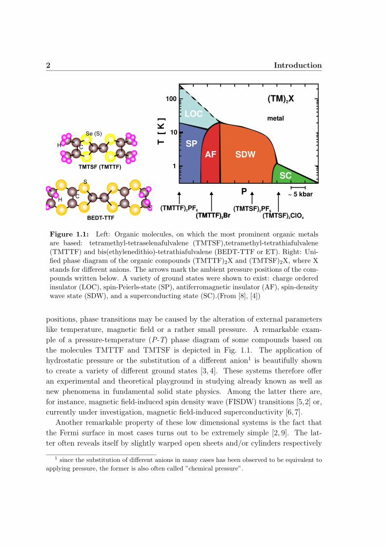
Generally, the organic molecules arrange themselves in stacks, forming conduct-
ing layers which are separated by insulating, mostly inorganic counterion layers. In
Fig. 1.1 examples of the most prominent organic molecules are depicted. Due to
the charge transfer between these planes, a strong coupling is provided, resulting
in stable crystalline materials. The layered character of the structure together with
various kinds of arrangements of the molecules within the conducting planes give
rise to very anisotropic, low-dimensional electron systems. This in turn causes a
variety of interesting properties.
On the one hand, low dimensional conducting systems are known to be unstable
with respect to the formation of various kinds of ordered ground states [2]. In the
field of organic metals virtually all possible ground states of a conducting system,
known up to date, were shown to exist. Moreover, it is known that, besides the
strong dependence of the electronic states on slight changes of the chemical com-
2 Introduction
S
Se (S)
C
H C
H
TMTSF (TMTTF)
BEDT-TTF
P
T
[ K
]1
100
10
SDWAF
SP
LOC
SC
(TM) X2
~ 5 kbar
metal
(TMTTF) PF2 6
(TMTTF) Br2
(TMTTF) Br2
(TMTSF) PF2 6
(TMTSF) ClO2 4
Figure 1.1: Left: Organic molecules, on which the most prominent organic metalsare based: tetramethyl-tetraselenafulvalene (TMTSF),tetramethyl-tetrathiafulvalene(TMTTF) and bis(ethylenedithio)-tetrathiafulvalene (BEDT-TTF or ET). Right: Uni-fied phase diagram of the organic compounds (TMTTF)2X and (TMTSF)2X, where Xstands for different anions. The arrows mark the ambient pressure positions of the com-pounds written below. A variety of ground states were shown to exist: charge orderedinsulator (LOC), spin-Peierls-state (SP), antiferromagnetic insulator (AF), spin-densitywave state (SDW), and a superconducting state (SC).(From [8], [4])
positions, phase transitions may be caused by the alteration of external parameters
like temperature, magnetic field or a rather small pressure. A remarkable exam-
ple of a pressure-temperature (P-T) phase diagram of some compounds based on
the molecules TMTTF and TMTSF is depicted in Fig. 1.1. The application of
hydrostatic pressure or the substitution of a different anion1 is beautifully shown
to create a variety of different ground states [3, 4]. These systems therefore offer
an experimental and theoretical playground in studying already known as well as
new phenomena in fundamental solid state physics. Among the latter there are,
for instance, magnetic field-induced spin density wave (FISDW) transitions [5,2] or,
currently under investigation, magnetic field-induced superconductivity [6, 7].
Another remarkable property of these low dimensional systems is the fact that
the Fermi surface in most cases turns out to be extremely simple [2, 9]. The lat-
ter often reveals itself by slightly warped open sheets and/or cylinders respectively
1 since the substitution of different anions in many cases has been observed to be equivalent toapplying pressure, the former is also often called ”chemical pressure”.
3
corresponding to a quasi-one-dimensional (Q1D) or a quasi-two-dimensional (Q2D)
conductivity of the charge carriers. This, in most cases, offers an easy experimen-
tal access for studying the electronic properties. For example, the measurement of
quantum oscillations has turned out to be an extremely powerful tool to determine
the Fermi surface geometry [9]. On the other hand, this simplicity of the Fermi
surface makes organic metals very nice model objects for theoretical investigations.
During the last decade the family of organic charge transfer salts α-(BEDT-
TTF)2MHg(SCN)4 (M=K,Tl,Rb) attracted attention due to several low temper-
ature anomalies found in magnetic field [10, 9]. While a density wave formation
could be figured out to occur below ≈ 10 K [11], there has been a long debate about
its real nature. No direct evidence for either a charge density or a spin density
modulation could be found. A recently proposed B-T phase diagram [12], however,
strongly favors a charge density wave (CDW) ground state in this organic system.
The most remarkable property of this CDW state would be the extremely low tran-
sition temperature and the correspondingly small energy gap. This allows available
static magnetic fields to strongly influence the CDW or, in other words, to investi-
gate the CDW state in an extremely wide range of its magnetic field-temperature
(B-T ) phase diagram. In particular, the first example of a modulated CDW-SDW
hybrid state is most probably found to exist at low temperatures in magnetic fields
above the paramagnetically limited ”conventional” CDW state [12]. This state is
an analogue to the theoretically proposed Fulde-Ferell-Larkin-Ovchinikov state pre-
dicted for low-dimensional superconductors [13, 14].
Besides this, measurements under hydrostatic pressure have shown that with ap-
plication of only a few kbar the density wave state likely becomes suppressed [15,16].
Pressure, therefore, can be used as a parameter to alter the electronic properties of
the system. Since these changes will very likely affect the density wave gap, one can
expect strong changes in the magnetic field effects. In addition, the resulting modu-
lation of the B-T phase diagram might further clarify the real nature of the density
wave state. The starting point of the present work, therefore, was the investigation
of the B-T phase diagrams at different hydrostatic pressures.
Within this work the electronic properties of the organic metal α-(BEDT-TTF)2-
KHg(SCN)4 were studied by means of resistance measurements under hydrostatic
pressure and additionally by combined resistance/magnetic-torque measurements at
ambient pressure. High magnetic fields up to 17 T were provided at the Walther-
Meissner-Institute and up to 30 T at the High Magnetic Field Laboratory in Greno-
4 Introduction
ble.
The results have indeed given further strong arguments for a CDW to exist at low
temperatures. It is shown that orbital effects appear in this low dimensional elec-
tron system in strong magnetic fields. These effects are for the first time observed
in a CDW system and give rise to several new phenomena. In particular, a series of
magnetic-field-induced CDW transitions has been observed for the first time.
Moreover, the presence of an additional, superconducting state under pressure is
demonstrated within this system.
Chapter 2
Theoretical Background
In this chapter we give a short introduction into the physics which is necessary for
the understanding of the present work. Since a complete theoretical description of
the different topics is beyond the scope of this thesis, the physics will be explained
in a rather qualitative manner.
2.1 Charge- and Spin-Density Waves (CDW, SDW)
2.1.1 Density Wave Instability in Low-Dimensional Elec-
tron Systems
A characteristic property of Q1D electron systems is their low-temperature instabil-
ity against a formation of either a charge- or a spin-density wave (CDW, SDW) with
a wave number q = 2kF ; where kF is the Fermi wave vector. This will be shortly
explained for the case of a CDW.
We assume a system of free (conduction) electrons to be exposed to an external
time-independent potential:
V (~r) =
∫V (~q)ei~q~rd~q. (2.1)
6 Theoretical Background
If this potential is not too strong, one can expect the change in the charge density
δϕ(q) to be proportional to the amplitude V (~q):
δϕ(~q) = χ(~q)V (~q). (2.2)
Here, the response function χ(q), also known as the Lindhard function [17], can be
derived from the perturbation theory [18] and, in d dimensions, is given by [19]:
χ(~q) =
∫d~k
(2π)d
fk − fk+q
εk − εk+q
, (2.3)
with εk = ε(k) being the electron dispersion relation and fk = f(εk) the Fermi-
Dirac distribution function. For a one-dimensional (1D) electron system, with a
linearized dispersion around the Fermi level, Eq. (2.3) at zero temperature can then
be evaluated near q = 2kF as:
χ(q) =−e2
π~vF
ln∣∣q + 2kF
q − 2kF
∣∣ = −e2n(εF ) ln∣∣q + 2kF
q − 2kF
∣∣, (2.4)
with e being the electron charge, vF the Fermi velocity and n(εF ) the carrier density
at the Fermi level. Obviously the response of a 1D electron system to an external
potential diverges on approaching the wave number 2kF . This, in turn, suggests by
self-consistency that a 1D electron gas itself becomes unstable against the formation
of a CDW with the wave number 2kF ; i.e. the perturbation potential is effectively
produced by the redistribution of the 1D carriers. This new periodic potential
appearing in the system can be shown to create energy gaps exactly at ±kF [19].
The energy of the electrons sitting near kF therefore decreases and the 1D system
eventually becomes insulating.
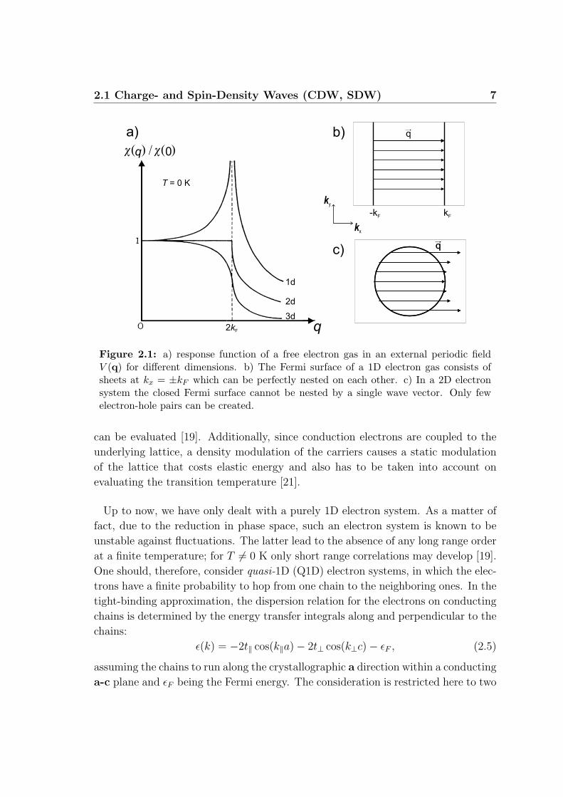
Looking back at Eq. (2.3) one understands the absence of such a divergence at
2kF for a free electron gas in the two-dimensional (2D) and three-dimensional (3D)
cases that is shown in Fig. 2.1 [20]. The divergence is caused by the presence of
electrons and holes on opposite sides of the Fermi surface, separated in k-space by
the same density wave vector. It now becomes evident that the response will only
diverge if many electron-hole pairs may be created. The bigger the part of the
Fermi surface is that ”nests” another part by shifting it with the wave vector of
the density wave, the stronger the response will be; and with it the energy gain of
the system by forming a density wave. Therefore the density wave vector is often
called nesting vector and we will adopt this designation below. On incorporating
a finite temperature into Eq. (2.3) the response of the system will become weaker
and a mean-field transition temperature, below which the density wave stabilizes,
2.1 Charge- and Spin-Density Waves (CDW, SDW) 7
kF-kF
q
kx
ky
b)
c)
a)
q
c( ) / c( )q 0
T = 0 K
1d
2d
3d
2kF
Figure 2.1: a) response function of a free electron gas in an external periodic fieldV (q) for different dimensions. b) The Fermi surface of a 1D electron gas consists ofsheets at kx = ±kF which can be perfectly nested on each other. c) In a 2D electronsystem the closed Fermi surface cannot be nested by a single wave vector. Only fewelectron-hole pairs can be created.
can be evaluated [19]. Additionally, since conduction electrons are coupled to the
underlying lattice, a density modulation of the carriers causes a static modulation
of the lattice that costs elastic energy and also has to be taken into account on
evaluating the transition temperature [21].
Up to now, we have only dealt with a purely 1D electron system. As a matter of
fact, due to the reduction in phase space, such an electron system is known to be
unstable against fluctuations. The latter lead to the absence of any long range order
at a finite temperature; for T 6= 0 K only short range correlations may develop [19].
One should, therefore, consider quasi-1D (Q1D) electron systems, in which the elec-
trons have a finite probability to hop from one chain to the neighboring ones. In the
tight-binding approximation, the dispersion relation for the electrons on conducting
chains is determined by the energy transfer integrals along and perpendicular to the
chains:
ε(k) = −2t‖ cos(k‖a)− 2t⊥ cos(k⊥c)− εF , (2.5)
assuming the chains to run along the crystallographic a direction within a conducting
a-c plane and εF being the Fermi energy. The consideration is restricted here to two
8 Theoretical Background
p
c
p
c
kc
ka
-kF kF
p
c
p
c
kc
ka
-kF kF
imperfectnesting
Q0
a) b)
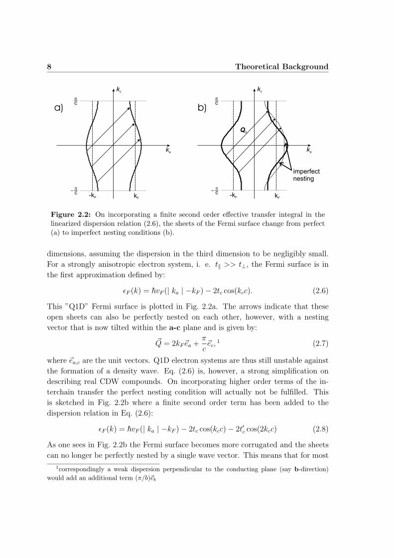
Figure 2.2: On incorporating a finite second order effective transfer integral in thelinearized dispersion relation (2.6), the sheets of the Fermi surface change from perfect(a) to imperfect nesting conditions (b).
dimensions, assuming the dispersion in the third dimension to be negligibly small.
For a strongly anisotropic electron system, i. e. t‖ >> t⊥, the Fermi surface is in
the first approximation defined by:
εF (k) = ~vF (| ka | −kF )− 2tc cos(kcc). (2.6)
This ”Q1D” Fermi surface is plotted in Fig. 2.2a. The arrows indicate that these
open sheets can also be perfectly nested on each other, however, with a nesting
vector that is now tilted within the a-c plane and is given by:
~Q = 2kF~ea +π
c~ec,
1 (2.7)
where ~ea,c are the unit vectors. Q1D electron systems are thus still unstable against
the formation of a density wave. Eq. (2.6) is, however, a strong simplification on
describing real CDW compounds. On incorporating higher order terms of the in-
terchain transfer the perfect nesting condition will actually not be fulfilled. This
is sketched in Fig. 2.2b where a finite second order term has been added to the
dispersion relation in Eq. (2.6):
εF (k) = ~vF (| ka | −kF )− 2tc cos(kcc)− 2t′c cos(2kcc) (2.8)
As one sees in Fig. 2.2b the Fermi surface becomes more corrugated and the sheets
can no longer be perfectly nested by a single wave vector. This means that for most
1correspondingly a weak dispersion perpendicular to the conducting plane (say b-direction)would add an additional term (π/b)~eb
2.1 Charge- and Spin-Density Waves (CDW, SDW) 9
CDWelectron
empty placeSDW
charg
edensity
charg
edensity
spin
density
0
spin
density
0
Figure 2.3: Qualitative arrangement of electrons in the CDW (left) and SDW states(right) in real space. Arrows show the direction of the spin. Below the resulting chargeand spin density modulations are shown for both cases.
regions on the Fermi surface the nesting becomes ”imperfect”. The effective energy
gap therefore decreases and so does the transition temperature Tc of the CDW
state. The density wave is then completely suppressed, i.e. Tc = 0 K, as soon as
free carriers appear on the Fermi surface [2]. To describe Q1D density wave systems
most theoretical investigations therefore consider the energy dispersion near the
Fermi level given by Eq. (2.8), where t′c can be regarded as an effective next-nearest-
neighbor transfer integral that introduces the imperfect nesting of the system.
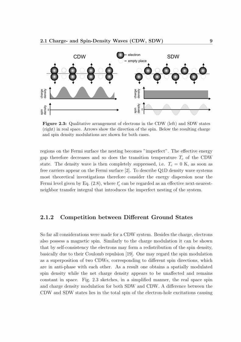
2.1.2 Competition between Different Ground States
So far all considerations were made for a CDW system. Besides the charge, electrons
also possess a magnetic spin. Similarly to the charge modulation it can be shown
that by self-consistency the electrons may form a redistribution of the spin density,
basically due to their Coulomb repulsion [19]. One may regard the spin modulation
as a superposition of two CDWs, corresponding to different spin directions, which
are in anti-phase with each other. As a result one obtains a spatially modulated
spin density while the net charge density appears to be unaffected and remains
constant in space. Fig. 2.3 sketches, in a simplified manner, the real space spin
and charge density modulation for both SDW and CDW. A difference between the
CDW and SDW states lies in the total spin of the electron-hole excitations causing
10 Theoretical Background
the diverging response.2 In the former electrons and holes at ±kF with opposite
spin directions interact with one another whereas in the SDW they have the same
spin direction [22]. As we shall see this has distinct consequences on applying an
external magnetic field to both systems. Besides the possibility of electron-hole
interaction (also known as Peierls channel) with excitations of finite momentum 2kF
there exists another competing mechanism of electron-electron pairing (the so-called
Cooper channel) with the total momentum equal to zero. These can be either the
superconducting singlet or triplet states. Which of these states eventually appears at
low temperatures depends on the strengths of electron-phonon and electron-electron
interactions. Theoretically this is considered in a strongly interacting electron gas
model by comparing the response functions for the different states [23,24]. We shall
not go here into details of this so-called g-ology model. In a qualitative consideration
one may say that [25]: if the electrostatic Coulomb repulsion dominates, there will
be preferably a SDW or a superconducting (spin-triplet) state. If, however, the
electrons mainly interact via phonons there will be an attracting force. In such a
case either a CDW or a superconducting (spin-singlet) state will form.
2.1.3 Density Waves in an External Magnetic Field
The present work is mostly focused on the influence of a magnetic field on (Q1D)
density wave systems. Here, we introduce the two basic effects, which are supposed
to occur.
Pauli Paramagnetic Effect
The main difference between SDW and CDW systems lies in the total spin of the
interacting electron-hole excitations. As one may immediately expect, an external
magnetic field, acting on the spins of the carriers, can have drastic consequences
on the stability of a density wave state. A simple consideration via the linearized
1D dispersion relation is sketched in Figs. 2.4 and 2.5. In a magnetic field the con-
duction band splits up into two sub-bands for electrons with opposite spins due to
2Note that density waves are actually not two-particle condensates. The annihilation of electronsat −kF and the creation of electrons at +kF and vice versa, leading to the diverging responsefunction, are theoretically considered as electron-hole excitations.
2.1 Charge- and Spin-Density Waves (CDW, SDW) 11
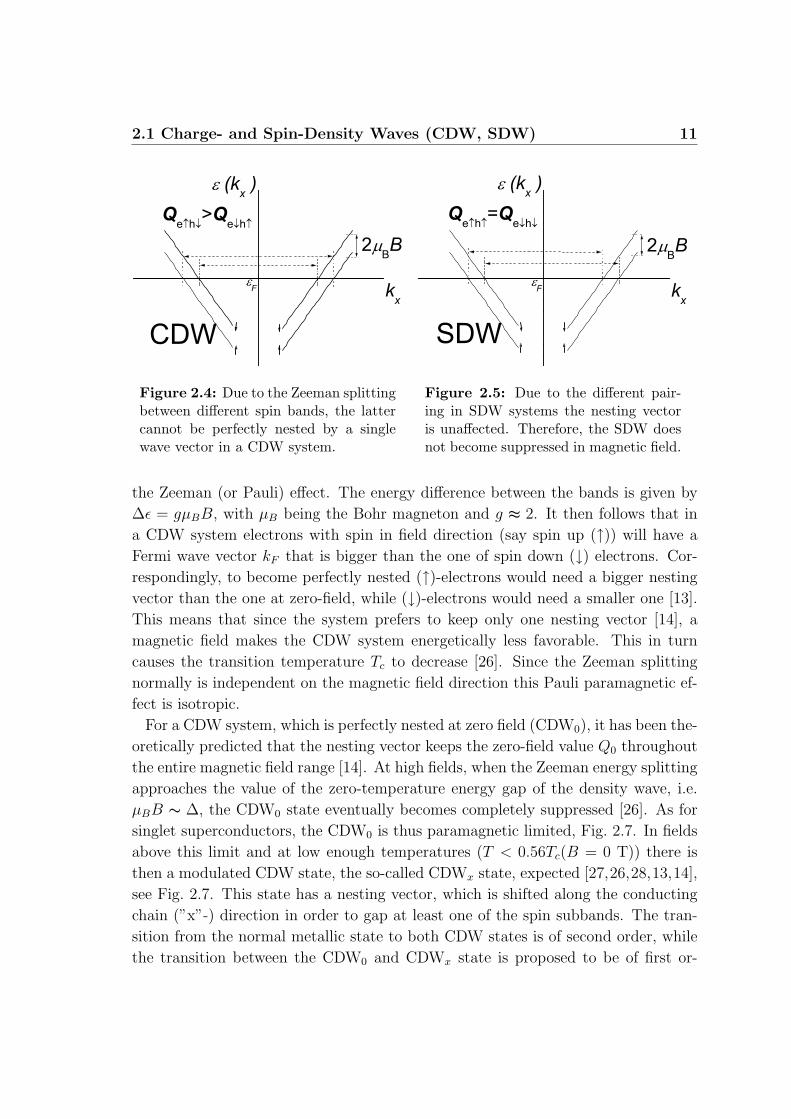
Figure 2.4: Due to the Zeeman splittingbetween different spin bands, the lattercannot be perfectly nested by a singlewave vector in a CDW system.
Figure 2.5: Due to the different pair-ing in SDW systems the nesting vectoris unaffected. Therefore, the SDW doesnot become suppressed in magnetic field.
the Zeeman (or Pauli) effect. The energy difference between the bands is given by
∆ε = gµBB, with µB being the Bohr magneton and g ≈ 2. It then follows that in
a CDW system electrons with spin in field direction (say spin up (↑)) will have a
Fermi wave vector kF that is bigger than the one of spin down (↓) electrons. Cor-
respondingly, to become perfectly nested (↑)-electrons would need a bigger nesting
vector than the one at zero-field, while (↓)-electrons would need a smaller one [13].
This means that since the system prefers to keep only one nesting vector [14], a
magnetic field makes the CDW system energetically less favorable. This in turn
causes the transition temperature Tc to decrease [26]. Since the Zeeman splitting
normally is independent on the magnetic field direction this Pauli paramagnetic ef-
fect is isotropic.
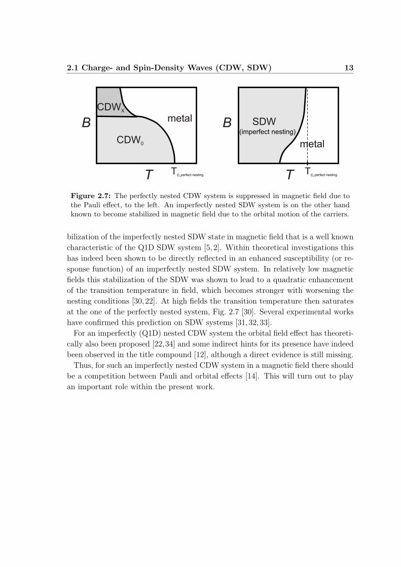
For a CDW system, which is perfectly nested at zero field (CDW0), it has been the-
oretically predicted that the nesting vector keeps the zero-field value Q0 throughout
the entire magnetic field range [14]. At high fields, when the Zeeman energy splitting
approaches the value of the zero-temperature energy gap of the density wave, i.e.
µBB ∼ ∆, the CDW0 state eventually becomes completely suppressed [26]. As for
singlet superconductors, the CDW0 is thus paramagnetic limited, Fig. 2.7. In fields
above this limit and at low enough temperatures (T < 0.56Tc(B = 0 T)) there is
then a modulated CDW state, the so-called CDWx state, expected [27,26,28,13,14],
see Fig. 2.7. This state has a nesting vector, which is shifted along the conducting
chain (”x”-) direction in order to gap at least one of the spin subbands. The tran-
sition from the normal metallic state to both CDW states is of second order, while
the transition between the CDW0 and CDWx state is proposed to be of first or-
12 Theoretical Background
B1 :
l h /eBc=
Dc etc= (4 / ) 1/BF
D Dc(B )1c(B ) <2
µ
B > B2 1 :
l
Fermisurface
real space motion
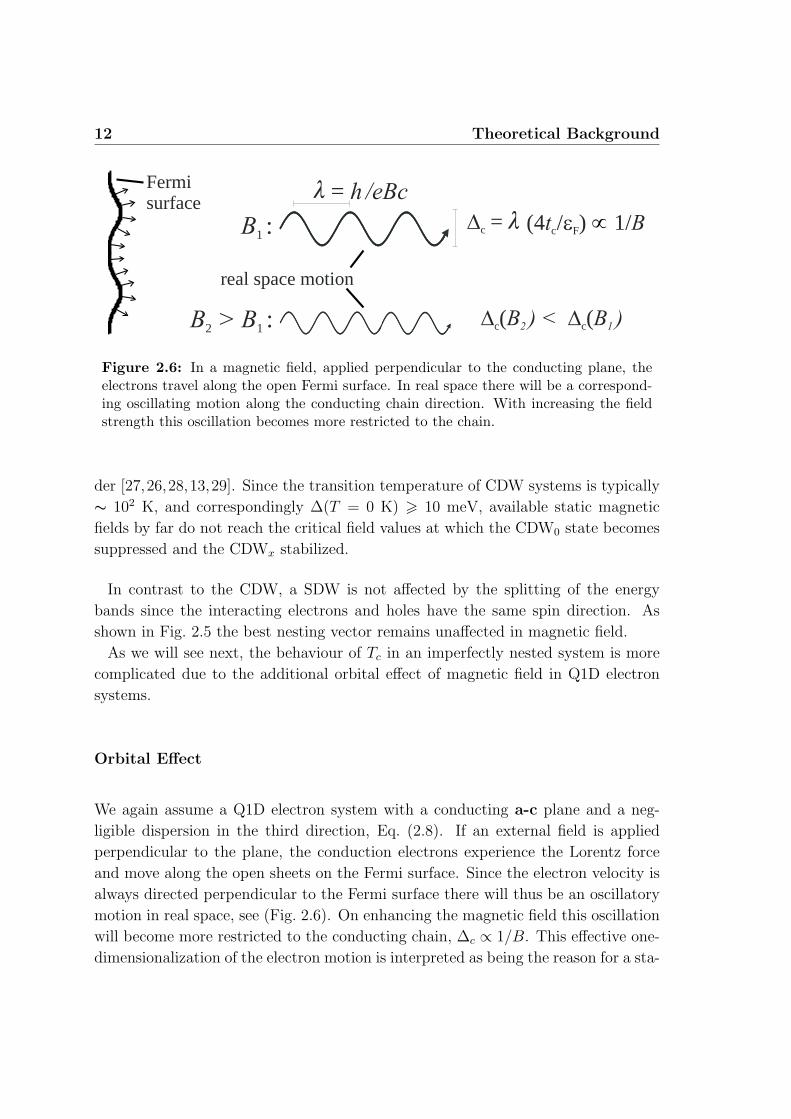
Figure 2.6: In a magnetic field, applied perpendicular to the conducting plane, theelectrons travel along the open Fermi surface. In real space there will be a correspond-ing oscillating motion along the conducting chain direction. With increasing the fieldstrength this oscillation becomes more restricted to the chain.
der [27,26,28,13,29]. Since the transition temperature of CDW systems is typically
∼ 102 K, and correspondingly ∆(T = 0 K) > 10 meV, available static magnetic
fields by far do not reach the critical field values at which the CDW0 state becomes
suppressed and the CDWx stabilized.
In contrast to the CDW, a SDW is not affected by the splitting of the energy
bands since the interacting electrons and holes have the same spin direction. As
shown in Fig. 2.5 the best nesting vector remains unaffected in magnetic field.
As we will see next, the behaviour of Tc in an imperfectly nested system is more
complicated due to the additional orbital effect of magnetic field in Q1D electron
systems.
Orbital Effect
We again assume a Q1D electron system with a conducting a-c plane and a neg-
ligible dispersion in the third direction, Eq. (2.8). If an external field is applied
perpendicular to the plane, the conduction electrons experience the Lorentz force
and move along the open sheets on the Fermi surface. Since the electron velocity is
always directed perpendicular to the Fermi surface there will thus be an oscillatory
motion in real space, see (Fig. 2.6). On enhancing the magnetic field this oscillation
will become more restricted to the conducting chain, ∆c ∝ 1/B. This effective one-
dimensionalization of the electron motion is interpreted as being the reason for a sta-
2.1 Charge- and Spin-Density Waves (CDW, SDW) 13
B
T
SDW(imperfect nesting)
metal
metalCDW0
B
TTc,perfect nesting
Tc,perfect nesting
CDWX
Figure 2.7: The perfectly nested CDW system is suppressed in magnetic field due tothe Pauli effect, to the left. An imperfectly nested SDW system is on the other handknown to become stabilized in magnetic field due to the orbital motion of the carriers.
bilization of the imperfectly nested SDW state in magnetic field that is a well known
characteristic of the Q1D SDW system [5,2]. Within theoretical investigations this
has indeed been shown to be directly reflected in an enhanced susceptibility (or re-
sponse function) of an imperfectly nested SDW system. In relatively low magnetic
fields this stabilization of the SDW was shown to lead to a quadratic enhancement
of the transition temperature in field, which becomes stronger with worsening the
nesting conditions [30,22]. At high fields the transition temperature then saturates
at the one of the perfectly nested system, Fig. 2.7 [30]. Several experimental works
have confirmed this prediction on SDW systems [31,32,33].
For an imperfectly (Q1D) nested CDW system the orbital field effect has theoreti-
cally also been proposed [22,34] and some indirect hints for its presence have indeed
been observed in the title compound [12], although a direct evidence is still missing.
Thus, for such an imperfectly nested CDW system in a magnetic field there should
be a competition between Pauli and orbital effects [14]. This will turn out to play
an important role within the present work.
14 Theoretical Background
2.2 Magnetic Quantum Oscillations
2.2.1 Conduction Electrons in a Magnetic Field
Solving the Schrodinger equation for a free electron gas in a magnetic field, applied
in z-direction, yields the energy eigenvalues [35]
En,kz = (n +1
2)~ωc +
~2
2mc
k2z , (2.9)
with the cyclotron frequency given by ωc = eB/mc, where mc is the cyclotron mass,
kz being the electron’s wave vector component parallel to the applied magnetic field
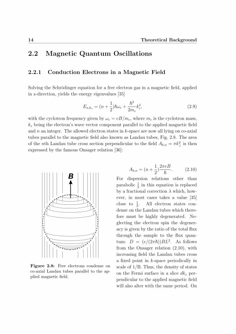
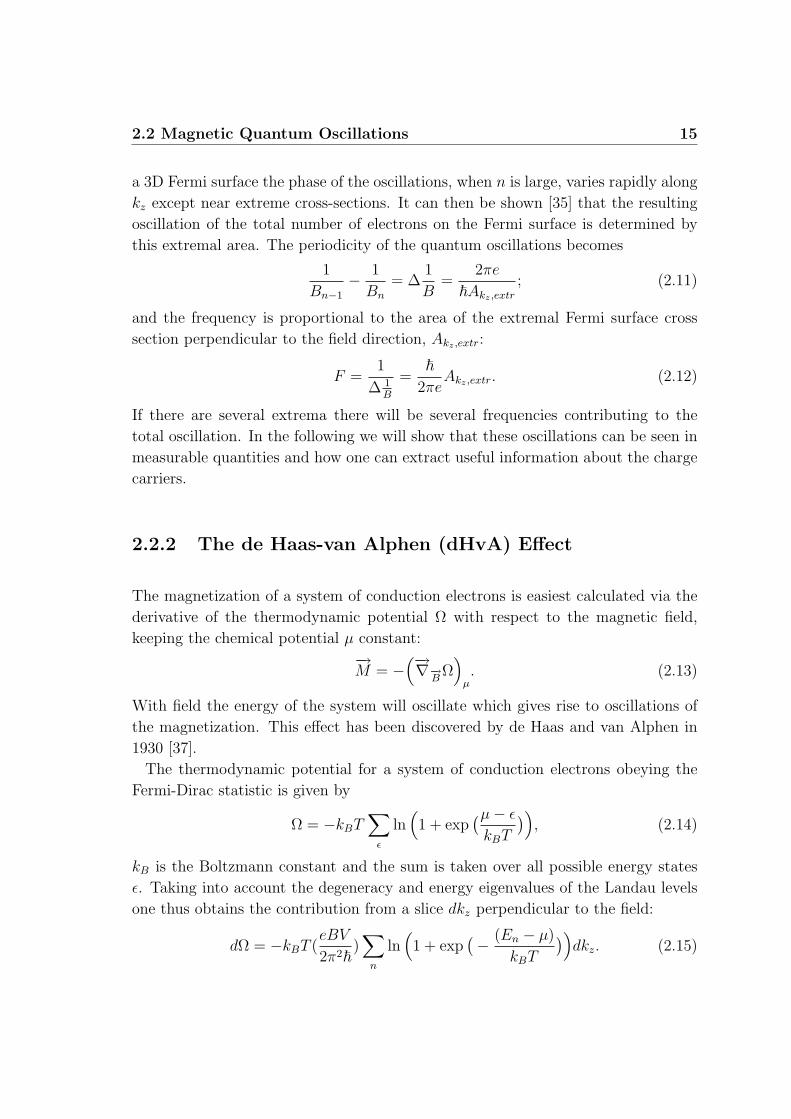
and n an integer. The allowed electron states in k-space are now all lying on co-axial
tubes parallel to the magnetic field also known as Landau tubes, Fig. 2.8. The area
of the nth Landau tube cross section perpendicular to the field Ak,n = πk2⊥ is then
expressed by the famous Onsager relation [36]:
B
Figure 2.8: Free electrons condense onco-axial Landau tubes parallel to the ap-plied magnetic field.
Ak,n = (n +1
2)2πeB
~. (2.10)
For dispersion relations other than
parabolic 12
in this equation is replaced
by a fractional correction λ which, how-
ever, in most cases takes a value [35]
close to 12. All electron states con-
dense on the Landau tubes which there-
fore must be highly degenerated. Ne-
glecting the electron spin the degener-
acy is given by the ratio of the total flux
through the sample to the flux quan-
tum: D = (e/(2π~))BL2. As follows
from the Onsager relation (2.10), with
increasing field the Landau tubes cross
a fixed point in k-space periodically in
scale of 1/B. Thus, the density of states
on the Fermi surface in a slice dkz per-
pendicular to the applied magnetic field
will also alter with the same period. On
2.2 Magnetic Quantum Oscillations 15
a 3D Fermi surface the phase of the oscillations, when n is large, varies rapidly along
kz except near extreme cross-sections. It can then be shown [35] that the resulting
oscillation of the total number of electrons on the Fermi surface is determined by
this extremal area. The periodicity of the quantum oscillations becomes
1
Bn−1
− 1
Bn
= ∆1
B=
2πe
~Akz ,extr
; (2.11)
and the frequency is proportional to the area of the extremal Fermi surface cross
section perpendicular to the field direction, Akz ,extr:
F =1
∆ 1B
=~
2πeAkz ,extr. (2.12)
If there are several extrema there will be several frequencies contributing to the
total oscillation. In the following we will show that these oscillations can be seen in
measurable quantities and how one can extract useful information about the charge
carriers.
2.2.2 The de Haas-van Alphen (dHvA) Effect
The magnetization of a system of conduction electrons is easiest calculated via the
derivative of the thermodynamic potential Ω with respect to the magnetic field,
keeping the chemical potential µ constant:
−→M = −
(−→∇−→
BΩ
)µ. (2.13)
With field the energy of the system will oscillate which gives rise to oscillations of
the magnetization. This effect has been discovered by de Haas and van Alphen in
1930 [37].
The thermodynamic potential for a system of conduction electrons obeying the
Fermi-Dirac statistic is given by
Ω = −kBT∑
ε
ln(1 + exp
(µ− ε
kBT
)), (2.14)
kB is the Boltzmann constant and the sum is taken over all possible energy states
ε. Taking into account the degeneracy and energy eigenvalues of the Landau levels
one thus obtains the contribution from a slice dkz perpendicular to the field:
dΩ = −kBT (eBV
2π2~)∑
n
ln(1 + exp
(− (En − µ)
kBT
))dkz. (2.15)
16 Theoretical Background
This equation can now be solved at T = 0 K using the Poisson or the Euler-
MacLaurin formulas [35]. At the final integration over kz only slices in the vicinity
of extremal areas add up constructively and the oscillation finally becomes:
Ω =
√e5
8π7~V B
52
meff
√A′′
∞∑p=1
1
p52
cos[2πp
(F
B− 1
2
)± π
4
](2.16)
where
A′′ =(∂2Akz
∂k2z
)kz=kz ,extr
(2.17)
From Eqs.(2.13) and (2.16) the magnetization components parallel and perpendic-
ular to the field can thus be derived as:
M‖ = −√
e5
2π5~V F
√B
meff
√A′′
∞∑p=1
1
p32
sin[2πp
(F
B− 1
2
)± π
4
](2.18)
M⊥ = − 1
F
∂F
∂θM‖ (2.19)
with meff being the effective cyclotron mass, which, in the absence of electron-
electron and electron-phonon interactions, equals to the band structure effective
mass.
On taking into account effects of finite temperature, electron scattering and Zee-
man spin splitting in magnetic field several independent reduction factors RT , RD
and RS have to be added to Eq. (2.18). Since it is especially these factors that give
information about the electronic properties of the system we will focus on them in the
next section. Including these damping factors into Eq. (2.18), one finally obtains the
famous Lifshitz-Kosevich (LK) equation describing the de Haas-van Alphen (dHvA)
oscillations in a 3D metallic electron system which, in the case of one extremal orbit,
reads:
M‖ = −√
e5
2π5~F√
B
meff
√A′′
∞∑p=1
RD(p)RT (p)RS(p)1
p3/2sin[2πp(
F
B− 1
2)± π
4] (2.20)
In polyvalent metals the FS generally exhibits more than one extremal cross-
sectional area. In that case, the total oscillatory part of the magnetization is simply
the sum over all contributions, each of them having the form (2.20), but with dif-
ferent parameters F , meff, A′′ and RT , RD, RS.
2.2 Magnetic Quantum Oscillations 17
2.2.3 Reduction Factors
The temperature reduction factor RT
At finite temperatures the Fermi distribution function
f(ε) =1
(1 + exp( ε−µkBT
))(2.21)
is no more step-like at the Fermi level. The whole system can now be treated as a
distribution of hypothetic metals, all at T = 0 K, having different Fermi energies and
hence contributing to the system with different frequencies. The superposition of
these oscillations, weighted according to the Fermi distribution, will cause a damping
of the initial oscillation. For the p-th harmonic this damping can be shown to be
expressed by the factor [35]:
RT (p) =αpm∗ T
B
sinh(αpm∗ TB
)(2.22)
with the constant
α =2π2kBme
~e≈ 14.69
T
K(2.23)
and the effective cyclotron mass m∗ in relative units of the free electron mass,
m∗ = meff/me. Thus, by fitting the experimentally observed temperature depen-
dent amplitude with Eq. (2.22), one can extract m∗. This mass is renormalized by
electron-electron and electron-phonon interactions.
The Dingle Factor RD
Conduction electrons possess a finite relaxation time τ mostly caused by lattice im-
perfections and impurities. Due to the uncertainty principle this leads to a broad-
ening of the otherwise δ-shaped Landau levels. Assuming this broadening to be
described by the Lorentzian distribution function the system can be treated in a
similar way as for finite temperature. The effect on the p-th harmonic of the oscil-
lation amplitude is then given by the Dingle reduction factor [35,38]:
RD = exp(− α
pmbTD
B
)(2.24)
18 Theoretical Background
with TD being the so-called Dingle temperature,
TD =~
2πkBτ. (2.25)
If the effective band mass mb is known, the evaluation of the Dingle temperature
via the field dependence of the oscillation amplitude is possible, and with it a mea-
sure of the crystal quality. Contrary to the effective cyclotron mass m∗ introduced
above the effective band mass mb is not renormalized due to electron-phonon inter-
actions. It should therefore be kept in mind that the use of m∗ instead of mb in
(2.24), that is a common procedure in the field of organic metals, can falsify the
evaluation of the Dingle temperature.
The Spin Reduction Factor RS
In a magnetic field, the Zeeman splitting lifts the spin degeneracy of the electron
energy. Accordingly, a Landau level of energy ε splits into sub-levels separated by
an energy gap
∆ε = g∗µBB; (2.26)
where µB = e~2me
, and g∗ is the Lande factor (for free electrons g∗=2.0023). These
two sets of Landau levels contribute to the oscillation at the same frequency but
with a phase difference given by
φ = 2π∆ε
~ωc
(2.27)
The superposition of these ”spin up” and ”spin down” oscillations causes an ad-
ditional spin reduction factor. For the p-th harmonic it may be written by [35]
Rs = cos(1
2pφ) = cos(
1
2pπg∗m∗) (2.28)
with m∗ being the effective cyclotron mass introduced above. Like m∗, g∗ is renor-
malized by electron-electron and electron-phonon interactions.
2.2.4 Shubnikov-de Haas (SdH) Oscillations
Shortly before the first experimental observation of the dHvA effect, Shubnikov and
de Haas [39] found quantum oscillations in transport measurements on a Bi single
2.2 Magnetic Quantum Oscillations 19
crystal. This phenomenon is therefore called Shubnikov-de Haas (SdH) oscillations.
The detailed theory of this effect, considering different kinds of scattering processes,
developed by Adams and Holstein in 1959 [40], is far beyond the scope of this
introductional chapter. However, a satisfactory description of the SdH effect is
usually obtained following Pippard’s idea that the scattering probability, and hence
the resistivity, is directly proportional to the density of states around the Fermi
level. The latter can be shown to be directly proportional to the field-derivative of
magnetization [35,41]:
D(µ) ∝(
mcB
Akz,extr
)2∂M
∂B. (2.29)
This gives an oscillatory part of the conductivity that may be expressed by:
σ
σ0
=∞∑
p=1
1
p12
ap cos
[2π
(F
B− 1
2
)± π
4
], (2.30)
where
ap ∝mcB
12
A′′ 12RT (p)RD(p)RS(p) (2.31)
and σ0 is the background conductivity. One sees, that the same damping factors as
for the dHvA effect can be used in order to extract properties of the electron system.
In the field of organic conductors this has been indeed shown in many cases to be
applicable [9].
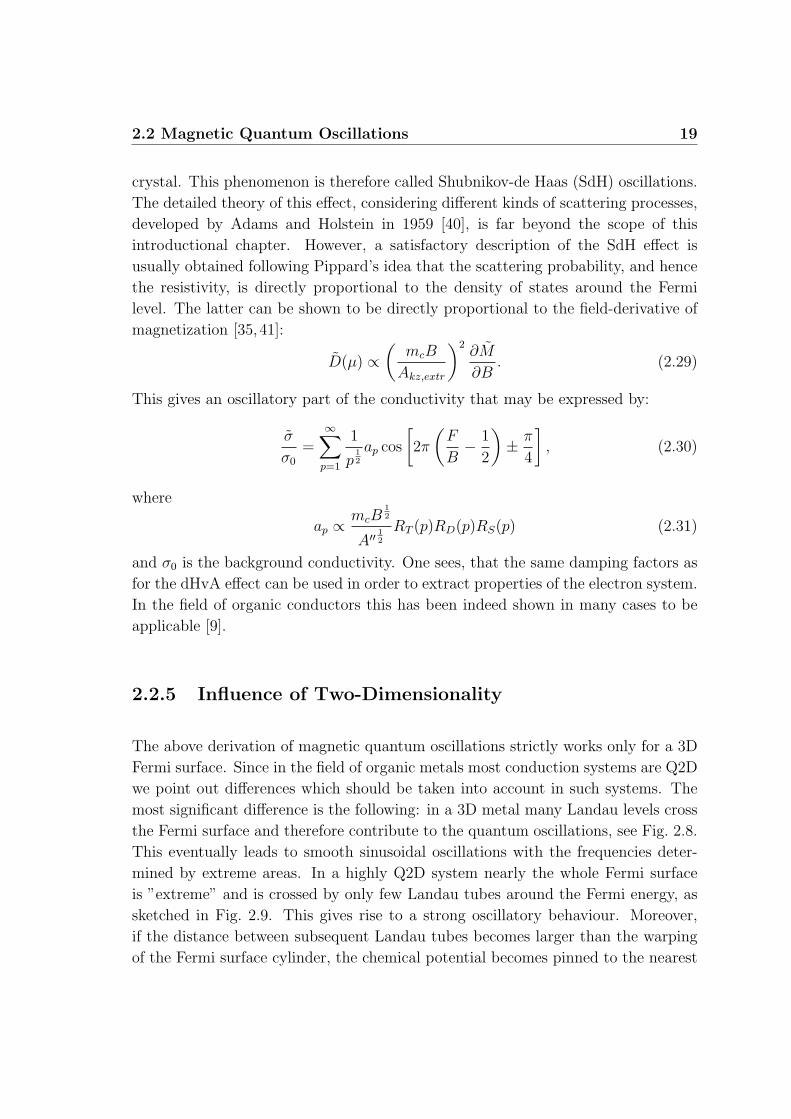
2.2.5 Influence of Two-Dimensionality
The above derivation of magnetic quantum oscillations strictly works only for a 3D
Fermi surface. Since in the field of organic metals most conduction systems are Q2D
we point out differences which should be taken into account in such systems. The
most significant difference is the following: in a 3D metal many Landau levels cross
the Fermi surface and therefore contribute to the quantum oscillations, see Fig. 2.8.
This eventually leads to smooth sinusoidal oscillations with the frequencies deter-
mined by extreme areas. In a highly Q2D system nearly the whole Fermi surface
is ”extreme” and is crossed by only few Landau tubes around the Fermi energy, as
sketched in Fig. 2.9. This gives rise to a strong oscillatory behaviour. Moreover,
if the distance between subsequent Landau tubes becomes larger than the warping
of the Fermi surface cylinder, the chemical potential becomes pinned to the nearest
20 Theoretical Background
Landau level: It increases with field until the highest level becomes completely un-
occupied and an abrupt jump down to the lower level occurs. This is immediately
reflected in a sawtooth shape of the dHvA signal, causing higher harmonic contents
of the oscillation [35]. On the other hand, if there are additional, non-quantized
bands on the Fermi surface, these will act as a carrier reservoir.
B
Figure 2.9: Only a few Landau levelscross a weakly warped cylindrical Fermisurface, characteristic of a Q2D metal,in a magnetic field applied in the leastconducting direction.
In the (hypothetical) limit of an infinite
reservoir the chemical potential becomes
again constant and the dHvA oscillation
takes the form of an inverse saw tooth [35].
However, since the carrier reservoirs in real
systems are finite such an extreme case
cannot be used to describe the shape of the
oscillations. Taking into account both the
oscillations from the quantized 2D band
and the reservoir bands, it can be shown
that the oscillation again takes a more sym-
metric shape in comparison to the above
extreme cases [42]. Noteworthy, the tem-
perature reduction factor might be affected
by the low dimensionality. However, rele-
vant changes in the amplitude of the first
harmonic are only expected at very low
temperatures and/or very high magnetic
fields, i.e. ~ωc/kT 10 [42, 43, 44]. Oth-
erwise, the extraction of the effective mass
from the temperature dependence of the
oscillations, as described above in sec. 2.2.3, should still be valid. The envelope
of the oscillations in a changing magnetic field, however, might be strongly affected
so that a determination of the Dingle temperature TD, as described above may be
incorrect. Concerning the SdH oscillations in very anisotropic Q2D systems the
situation will become even more complicated as will be pointed out in this work.
2.2 Magnetic Quantum Oscillations 21
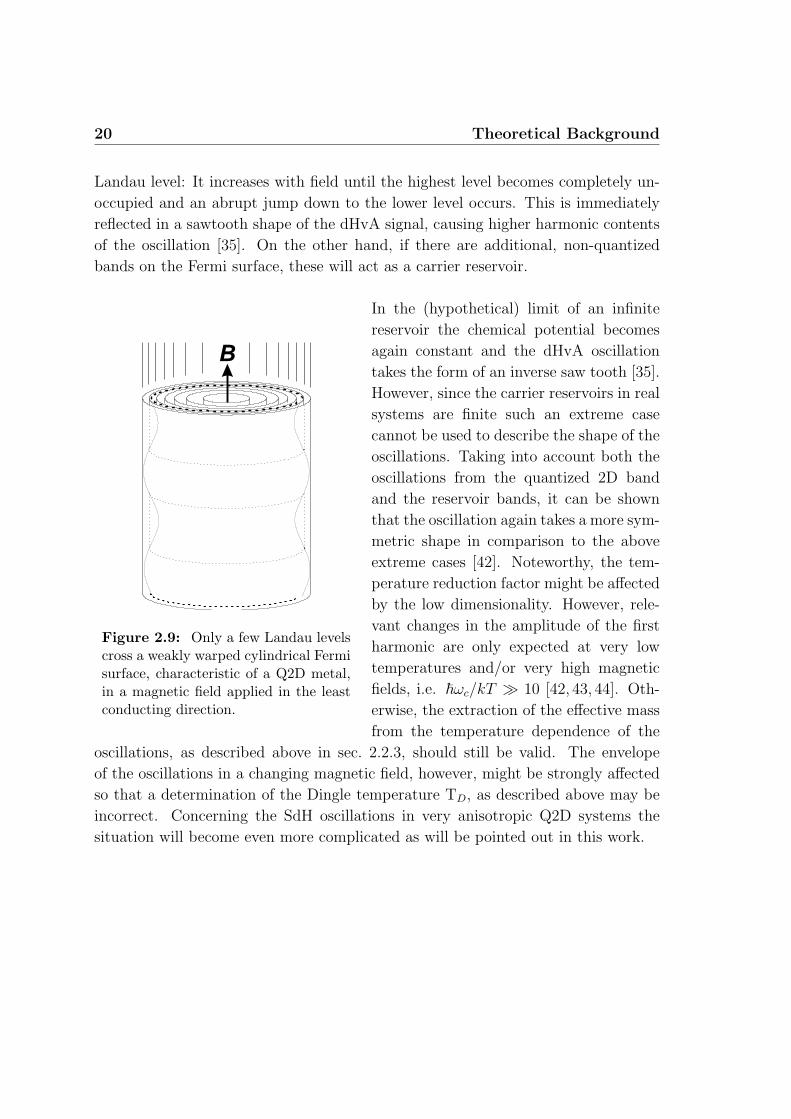
b
a
Figure 2.10: Example of magnetic breakdown between open and closed trajectories:In magnetic field the carriers on the Fermi surface have a finite probability to tunnelbetween different bands, dashed lines. This may lead to additional closed orbits, here:β-orbit, dotted line.
2.2.6 Magnetic Breakdown
The LK formula derived above only considers electrons on well defined closed orbits
on the Fermi surface. There exists, however, another possibility in magnetic field
for the electrons in multiband metals to run on closed pockets on the Fermi surface
by tunneling processes between the bands, that is called magnetic breakdown (MB).
Fig. 2.10 illustrates this phenomenon in the case of coexisting open and closed parts
of the Fermi surface, that is typically found in many organic metals. If the energy
barrier εg between neighboring trajectories is small in comparison to the Fermi
energy there will be a finite probability for the electrons in a strong magnetic field
to tunnel between the bands. This may lead to an additional orbit (here: β-orbit)
contributing to the quantum oscillations. The probability of MB can be expressed
as [45]
P = exp
(−B0
B
), (2.32)
where the MB field parameter B0 is defined as
B0 ≈m∗ε2
g
e~εF
. (2.33)
With increasing field, referring to Fig. 2.10, more electrons will tunnel between the
bands causing a bigger contribution to the β-oscillations while less electrons run on
the semiclassical trajectories along the open and closed parts on the Fermi surface.
22 Theoretical Background
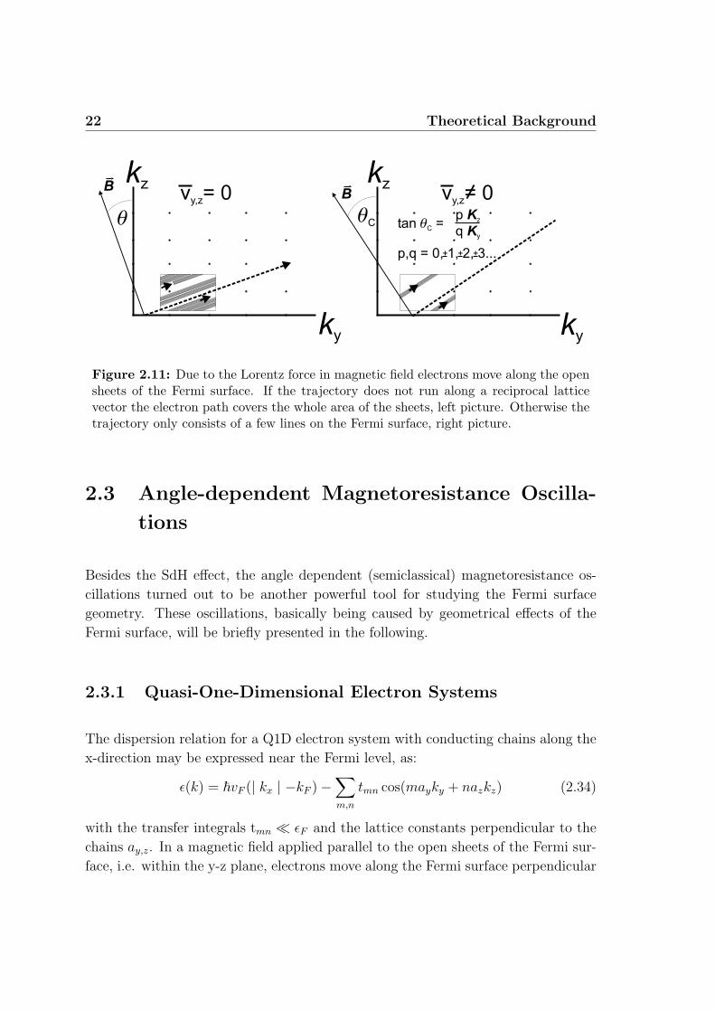
v = 0y,z v = 0y,z
ky ky
kzBB
q qC
kz
tan =qC
p Kz
q Ky
p,q = 0, 1, 2, 3...+ ++
Figure 2.11: Due to the Lorentz force in magnetic field electrons move along the opensheets of the Fermi surface. If the trajectory does not run along a reciprocal latticevector the electron path covers the whole area of the sheets, left picture. Otherwise thetrajectory only consists of a few lines on the Fermi surface, right picture.
2.3 Angle-dependent Magnetoresistance Oscilla-
tions
Besides the SdH effect, the angle dependent (semiclassical) magnetoresistance os-
cillations turned out to be another powerful tool for studying the Fermi surface
geometry. These oscillations, basically being caused by geometrical effects of the
Fermi surface, will be briefly presented in the following.
2.3.1 Quasi-One-Dimensional Electron Systems
The dispersion relation for a Q1D electron system with conducting chains along the
x-direction may be expressed near the Fermi level, as:
ε(k) = ~vF (| kx | −kF )−∑m,n
tmn cos(mayky + nazkz) (2.34)
with the transfer integrals tmn εF and the lattice constants perpendicular to the
chains ay,z. In a magnetic field applied parallel to the open sheets of the Fermi sur-
face, i.e. within the y-z plane, electrons move along the Fermi surface perpendicular
2.3 Angle-dependent Magnetoresistance Oscillations 23
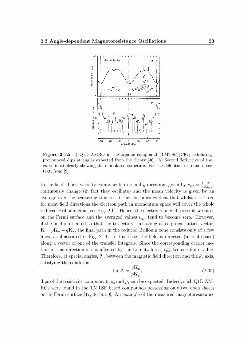
Figure 2.12: a) Q1D AMRO in the organic compound (TMTSF)2ClO4 exhibitingpronounced dips at angles expected from the theory [46]. b) Second derivative of thecurve in a) clearly showing the modulated structure. For the definition of p and q seetext, from [9].
to the field. Their velocity components in z and y direction, given by vy,z = 1~
∂ε∂ky,z
,
continously change (in fact they oscillate) and the mean velocity is given by an
average over the scattering time τ . It then becomes evident that whilst τ is large
for most field directions the electron path in momentum space will cover the whole
reduced Brillouin zone, see Fig. 2.11. Hence, the electrons take all possible k-states
on the Fermi surface and the averaged values vy,z tend to become zero. However,
if the field is oriented so that the trajectory runs along a reciprocal lattice vector,
K = pKy + qKz, the final path in the reduced Brillouin zone consists only of a few
lines, as illustrated in Fig. 2.11. In this case, the field is directed (in real space)
along a vector of one of the transfer integrals. Since the corresponding carrier mo-
tion in this direction is not affected by the Lorentz force, vy,z keeps a finite value.
Therefore, at special angles, θc, between the magnetic field direction and the kz axis,
satisfying the condition
tan θc =qKz
pKy
, (2.35)
dips of the resistivity components ρy and ρz can be expected. Indeed, such Q1D AM-
ROs were found in the TMTSF based compounds possessing only two open sheets
on its Fermi surface [47,48,49,50]. An example of the measured magnetoresistance
24 Theoretical Background
BB
B
a) c)b) qn=1
Figure 2.13: Closed electron orbits on a slightly warped cylindrical Fermi surface atdifferent magnetic field directions: a),b),c). Only for certain field directions (b) all orbitareas are the same.
is given in Fig. 2.12 for the organic metal (TMTSF)2ClO4.
2.3.2 Quasi-Two-Dimensional Electron Systems
Besides the Q1D AMRO there exists another angular effect arising from a cylindrical
Fermi surface, i.e. a Q2D electron system [51, 52, 53, 54]. By contrast to the Q1D
AMRO, described above, these happen to appear only in the interplane resistance
[55]. The simplest energy dispersion for a Q2D system may be expressed as:
ε(k) =~2
2m∗ (k2x + k2
y)− 2t⊥ cos(azkz) (2.36)
The Fermi surface is thus represented by a cylinder slightly warped in kz-direction.
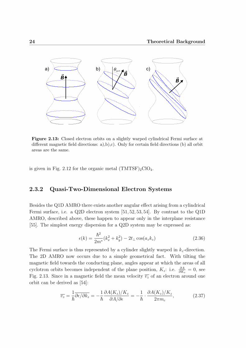
The 2D AMRO now occurs due to a simple geometrical fact. With tilting the
magnetic field towards the conducting plane, angles appear at which the areas of all
cyclotron orbits becomes independent of the plane position, Kz: i.e. ∂A∂Kz
= 0, see
Fig. 2.13. Since in a magnetic field the mean velocity vz of an electron around one
orbit can be derived as [54]:
vz =1
~∂ε/∂kz = −1
~∂A(Kz)/Kz
∂A/∂ε= −1
~· ∂A(Kz)/Kz
2πmc
, (2.37)
2.3 Angle-dependent Magnetoresistance Oscillations 25
inte
rlayer
resis
tance
angle q
----
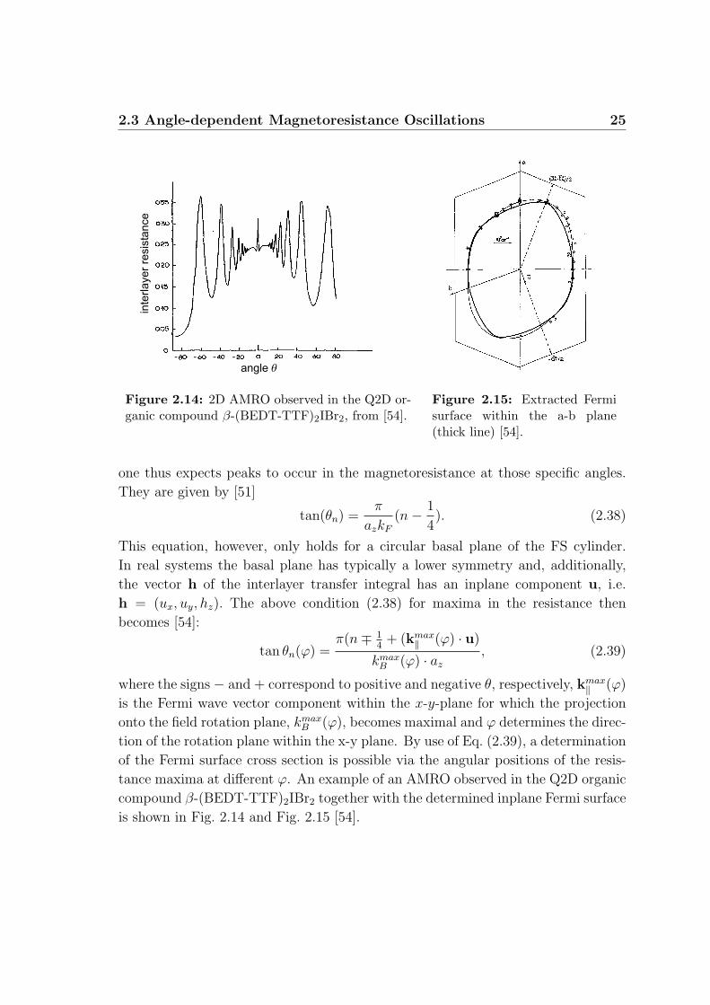
Figure 2.14: 2D AMRO observed in the Q2D or-ganic compound β-(BEDT-TTF)2IBr2, from [54].
Figure 2.15: Extracted Fermisurface within the a-b plane(thick line) [54].
one thus expects peaks to occur in the magnetoresistance at those specific angles.
They are given by [51]
tan(θn) =π
azkF
(n− 1
4). (2.38)
This equation, however, only holds for a circular basal plane of the FS cylinder.
In real systems the basal plane has typically a lower symmetry and, additionally,
the vector h of the interlayer transfer integral has an inplane component u, i.e.
h = (ux, uy, hz). The above condition (2.38) for maxima in the resistance then
becomes [54]:
tan θn(ϕ) =π(n∓ 1
4+ (kmax
‖ (ϕ) · u)
kmaxB (ϕ) · az
, (2.39)
where the signs − and + correspond to positive and negative θ, respectively, kmax‖ (ϕ)
is the Fermi wave vector component within the x-y-plane for which the projection
onto the field rotation plane, kmaxB (ϕ), becomes maximal and ϕ determines the direc-
tion of the rotation plane within the x-y plane. By use of Eq. (2.39), a determination
of the Fermi surface cross section is possible via the angular positions of the resis-
tance maxima at different ϕ. An example of an AMRO observed in the Q2D organic
compound β-(BEDT-TTF)2IBr2 together with the determined inplane Fermi surface
is shown in Fig. 2.14 and Fig. 2.15 [54].
26 Theoretical Background
2.4 Kohler’s Rule
In a magnetic field−→B the motion of an electron is affected by the Lorentz force,
causing (at least for closed Fermi surfaces) a curving of the electron trajectory in
the plane perpendicular to the applied field. The characteristic size of this curving
is given by the magnetic length (Larmor radius in the case of closed orbits) which is
inversely proportional to the magnetic field B and is given by the electron velocity
divided by the cyclotron frequency ωc = eBmc
. As a result, the effective mean free path
in the direction of the electric field decreases and the resistivity ρ in that direction
increases. For anisotropic metals it has turned out to be extremely difficult to
calculate the field dependence of the resistivity in moderate fields, i.e. fields where
ωcτ ∼ 1, τ being the electron scattering time. Because of this, use is sometimes made
of Kohler’s rule, which is a similarity law for the magnetoresistance. A summary of
its derivation given by Pippard [56] is presented below.
A bunch of electrons, all having the same initial wave vector−→k on the Fermi
surface, give a current contribution in a steady electric field−→E (with or without an
applied magnetic field), that can be written as [56]:
δ−→J =
e2−→E δ−→S
4π3~−→L , (2.40)
δ−→S being an element of the Fermi surface.
−→L , the effective path, is defined as
the mean vector distance traveled by each electron from the bunch until the cen-
troid of them comes to rest due to scattering. One can treat this effective path
as a k-dependent mean free length for electrons in a given magnetic field. In an
applied magnetic field, this bunch of electrons moves on orbits, with linear dimen-
sions inversely proportional to B, and dissipate by collisions. The idea is to look
what would happen, if the scattering rate is increased by a factor a, for example by
adding impurities, and at the same time the magnetic field B is also enhanced to
the same amount, B′ = aB. If these ”extra” collisions, causing the reduced scat-
tering time τ ′ = τ/a, are of the same sort, the pattern of the electronic behaviour
should be simply scaled down without changing the character. This implies, that
the scattering rate does not depend on the magnetic field. In this case the effective
path L and all components of the conductivity will be divided by a and any mea-
sured resistivity multiplied by this factor, ρ′(B) = aρ(B). This means that if we
keep the ratio B/ρzero-field constant, on the one hand the probability of an electron
to be scattered over one cycle of the orbit remains constant (ωcτ = const.). Then
2.4 Kohler’s Rule 27
on the other hand, the magnetoresistance, which is the resistivity normalized to its
zero-field value, remains the same; i.e.:
ρ′(B)
ρ′zero-field
=aρ(B)
aρzero-field
=ρ(B)
ρzero-field
= const. (2.41)
In other words, the magnetoresistance is a general function of the magnetic field
divided by the zero-field resistance:
∆ρ(B)
ρzero-field
= F (B
ρzero-field
); ∆ρ = ρ(B)− ρzero-field. (2.42)
This is Kohler’s rule.
Since this law is derived using certain assumptions, one should be careful as to
which cases it can or cannot be used. Some examples for which the rule fails are
given in the following:
• If the scattering time is field dependent, Kohler’s rule is no longer valid. This
would be the case, for example, when the scattering is due to magnetic impu-
rities.
• Effects of orbit quantization will also break the law because the scattering rate
becomes field dependent in a way that it starts oscillating.
• In the case of a magnetic breakdown, the electrons have a finite probability
(depending on the magnetic field) to switch to another band, that will cause
a different current distribution in real space and therefore a deviation from
Kohler’s rule.
• If there is a large content of phonon scattering, the modification of the phonon
spectrum with changing the temperature results in an altered scattering pat-
tern. One of the basic assumptions made for Kohler’s rule is not fulfilled.
• If there is a phase transition to another (conducting) state on changing the
temperature and/or magnetic field, the scattering pattern will be altered.
Therefore, Kohler‘s rule in some cases can even be used for the determina-
tion of such phase transitions.

28 Theoretical Background
Chapter 3
The Organic Metal
α-(BEDT-TTF)2KHg(SCN)4
3.1 Synthesis
Single crystals of α-(BEDT-TTF)2KHg(SCN)4 are prepared using standard electro-
chemical techniques [57, 2]. The salts KSCN and Hg(SCN)2 are dissolved in a mix-
ture of (1,1,2)trichlorethane and methanol. Organic BEDT-TTF (often shortened
to ET) molecules are then electrochemically oxidized in this solution by applying
a constant current between Pt-electrodes, the initial salts serving as electrolytes.
To initiate crystal growth the current density is kept at a very low level of about
1-2 µA/cm2 while the temperature is held at the constant value of 20C. After 2-4
weeks small plate-like samples with a typical size of 0.5*0.5*0.1 mm3 appear on the
Pt-anode. In our measurements samples were taken from different batches, some
prepared by N.D.Kushch in the WMI , others by H.Muller at the ESRF in Grenoble.
3.2 Crystal Structure
All the charge transfer salts (BEDT-TTF)mXn have a nearly planar donor molecule
BEDT-TTF due to an extended π-electron orbital system [58,2]. The crystal struc-
30 The Organic Metal α-(BEDT-TTF)2KHg(SCN)4
K
Figure 3.1: Crystal structure of α-(BEDT-TTF)2KHg(SCN)4. The BEDT-TTFmolecules arrange in conducting planes which are separated by insulating anion lay-ers [57].
ture of α-(BEDT-TTF)2KHg(SCN)4 is illustrated in Fig. 3.1. It contains conducting
cation-radical layers of BEDT-TTF, within the crystallographic a-c plane, alternat-
ing along the b-axis with relatively thick polymeric insulating anion layers [57].
Within the BEDT-TTF sheets, the molecules are connected via π-orbitals between
the sulfur atoms. The transfer of charge between the layers results in stable crys-
talline materials. In the anion sheets each SCN molecule forms a bridge between
the K+ and Hg2+ cations leading to a polymeric network in the a-c plane. This
layered structure is typical for (BEDT-TTF)+2 X− compounds. Depending on dif-
ferent anions, the BEDT-TTF molecules are arranged within the layer in different
formations, which are denoted by Greek characters. In the α-type salt with the
anion [KHg(SCN)4]− the BEDT-TTF donors are ordered in stacks, labeled A and
3.3 Fermi Surface and Band Structure 31
Figure 3.2: Left: Inplane arrangement of the ET molecules viewed along their molecu-lar axis. The dotted lines between the molecules stand for the different transfer integralsin the stack direction (ci) and interstack direction (pi). Right: Molecular chains in thea-direction (black) give rise to a Q1D electron motion.
B, with a characteristic ”fish bone” pattern (Fig. 3.2). The molecules in stack B
are located in non-equivalent inversion centres marked II and III, whereas in stack
A they are in equivalent positions I. Therefore the unit cell contains two formula
units. The crystal structure is triclinic with the parameters a=10.082A, b=20.565A,
c=9.973A, α=103.7, β=90.91, γ=93.06 and a cell volume of 1997 A3.
3.3 Fermi Surface and Band Structure
Since two BEDT-TTF molecules give one electron to the anion leaving a hole behind,
there are two holes in one unit cell, the latter containing four BEDT-TTF molecules.
This means, that there will exist four HOMO(= highest occupied molecular orbital)
bands, which are filled with six electrons per unit cell. Due to the fact that the up-
per two bands (in energy scale) overlap [57], both of them cross the Fermi level, i.e.
the BEDT-TTF sheets possess a metallic character. Small overlaps of the molecular
orbitals of adjacent BEDT-TTF layers lead to an electron exchange between them
and thus to a finite conductivity perpendicular to the highly conducting planes. The
band structure determined by Mori et al. [59] via an extended Huckel tight-binding
calculation, based on the crystal structure at 100 K, and the corresponding Fermi
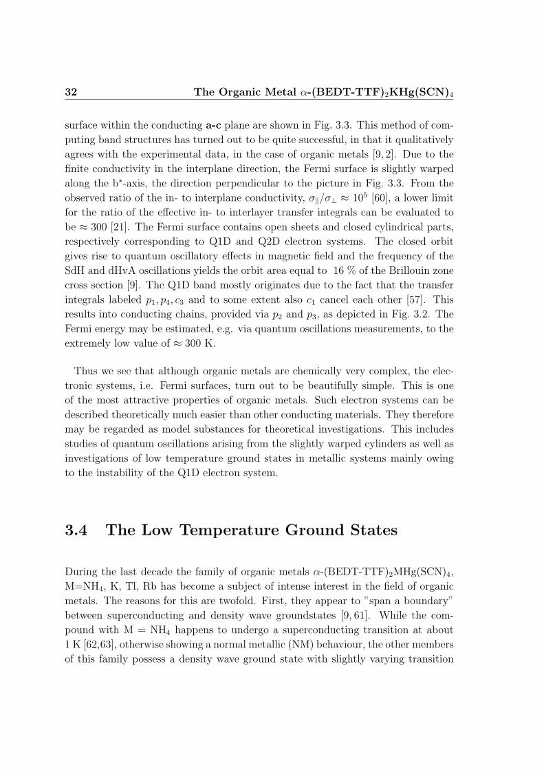
32 The Organic Metal α-(BEDT-TTF)2KHg(SCN)4
surface within the conducting a-c plane are shown in Fig. 3.3. This method of com-
puting band structures has turned out to be quite successful, in that it qualitatively
agrees with the experimental data, in the case of organic metals [9, 2]. Due to the
finite conductivity in the interplane direction, the Fermi surface is slightly warped
along the b∗-axis, the direction perpendicular to the picture in Fig. 3.3. From the
observed ratio of the in- to interplane conductivity, σ‖/σ⊥ ≈ 105 [60], a lower limit
for the ratio of the effective in- to interlayer transfer integrals can be evaluated to
be ≈ 300 [21]. The Fermi surface contains open sheets and closed cylindrical parts,
respectively corresponding to Q1D and Q2D electron systems. The closed orbit
gives rise to quantum oscillatory effects in magnetic field and the frequency of the
SdH and dHvA oscillations yields the orbit area equal to 16 % of the Brillouin zone
cross section [9]. The Q1D band mostly originates due to the fact that the transfer
integrals labeled p1, p4, c3 and to some extent also c1 cancel each other [57]. This
results into conducting chains, provided via p2 and p3, as depicted in Fig. 3.2. The
Fermi energy may be estimated, e.g. via quantum oscillations measurements, to the
extremely low value of ≈ 300 K.
Thus we see that although organic metals are chemically very complex, the elec-
tronic systems, i.e. Fermi surfaces, turn out to be beautifully simple. This is one
of the most attractive properties of organic metals. Such electron systems can be
described theoretically much easier than other conducting materials. They therefore
may be regarded as model substances for theoretical investigations. This includes
studies of quantum oscillations arising from the slightly warped cylinders as well as
investigations of low temperature ground states in metallic systems mainly owing
to the instability of the Q1D electron system.
3.4 The Low Temperature Ground States
During the last decade the family of organic metals α-(BEDT-TTF)2MHg(SCN)4,
M=NH4, K, Tl, Rb has become a subject of intense interest in the field of organic
metals. The reasons for this are twofold. First, they appear to ”span a boundary”
between superconducting and density wave groundstates [9, 61]. While the com-
pound with M = NH4 happens to undergo a superconducting transition at about
1 K [62,63], otherwise showing a normal metallic (NM) behaviour, the other members
of this family possess a density wave ground state with slightly varying transition
3.4 The Low Temperature Ground States 33
Figure 3.3: Band structure and Fermi surface of α-(BEDT-TTF)2KHg(SCN)4 calcu-lated by Mori et al. [59]. For newer results see also ref. [57].
temperatures of 8 K (M=K), 9 K (M=Tl) and 12 K(M=Rb). After a long series of
investigations there is nowadays a general agreement that it is the charge density
which becomes modulated at low temperatures. Since the transition temperatures
of these compounds are uniquely low, an investigation of a CDW system becomes
possible in an extremely wide range of its B-T phase diagram, giving the other main
reason for the broad interest in these compounds. This section gives a short review
on the most important observations on the low temperature state known by the
beginning of this work, mainly focusing on the M = K salt.
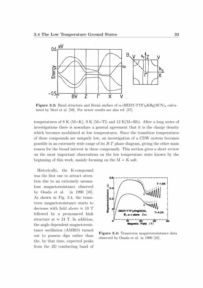
Figure 3.4: Transverse magnetoresistance dataobserved by Osada et al. in 1990 [10].
Historically, the K-compound
was the first one to attract atten-
tion due to an extremely anoma-
lous magnetoresistance observed
by Osada et al. in 1990 [10].
As shown in Fig. 3.4, the trans-
verse magnetoresistance starts to
decrease with field above ≈ 10 T
followed by a pronounced kink
structure at ≈ 24 T. In addition,
the angle dependent magnetoresis-
tance oscillation (AMRO) turned
out to possess dips rather than
the, by that time, expected peaks
from the 2D conducting band of

34 The Organic Metal α-(BEDT-TTF)2KHg(SCN)4
G
Z
X
MS
Q
new closed orbit
new open trajectory
Figure 3.5: Left: Fermi surface of the normal metallic state calculated by Rousseauet al. [57]. Right: Within the CDW state the open sheets on the Fermi surface becomecompletely nested, while the cylindrical parts are reconstructed. The new periodicitygiven by the nesting vector creates new closed orbits and open trajectories.
the electron system, introduced in section 2.3. Indeed, the AMROs in the low tem-
perature state of these α-salts turned out to be caused by open sheets on the Fermi
surface [11,64]. This type of AMRO had already been observed in the Q1D organic
metal (TMTSF)2ClO4 [65,48,49,50] and could be reasonably described by a theory
developed by Osada et al. in 1992 [46].
Surprisingly, these open sheets were found to be tilted by an angle of ≈ 20
within the conducting plane with respect to the proposed ones from band structure
calculations [59, 57], Fig. 3.3. From the observed data it was possible to determine
the periodicity of an additional periodic potential that has to be superposed on
the system at low temperatures. Kartsovnik et al. [11] attributed this additional
potential to a Peierls-type transition of the system that causes a reconstruction of the
Fermi surface. How this schematically looks like within the a-c-plane is depicted in
Fig. 3.5. The wave vector of the additional potential nests the Q1D part of the Fermi
surface completely and therefore the Q1D carriers become gapped. The remaining
Q2D part is then periodically shifted by the nesting vector building a reconstructed
Fermi surface. As a result, there exist open sheets on the Fermi surface, running
along the nesting wave vector and in between smaller pockets get formed. Indeed,
Kartsovnik et al. in the same work presented additional SdH frequencies which were
then attributed to these small pockets. As is evident, the orientation of the new Q1D
sheets and the area of the new pockets will strongly depend on the exact coordinates
of the nesting vector. The latter was proposed by Kartsovnik et al. [64, 66] to be
3.4 The Low Temperature Ground States 35
expressed by:
Q =1
8Ka +
1
8Kc +
1
6Kb, (3.1)
which is tilted within the plane from the c-axis by ≈ 20, Ka,c,b being the recipro-
cal lattice vectors. However, since the nesting vector determined by other groups
from AMRO measurements for unclear reasons are slightly more tilted, 27 [67] and
30 [68], there is up to now no general agreement about how the Fermi surface is
reconstructed.
After this finding of a nested Fermi surface a long debate started about the nature
of the density wave state. Due to a drop in the inplane magnetic susceptibility on
crossing the phase boundary at ≈ 8 K, while the interplane component remains
unchanged, Sasaki et al. [69] concluded that the low temperature state orders anti-
ferromagnetically and therefore should emerge due to the presence of a SDW. Such
a suggestion was then supported by µSR measurements [70], in which possible or-
dered magnetic moments of≈ 10−3µB were predicted. However, besides the fact that
this was the only µSR study reported on this compound, ESR [71] and NMR [72]
investigations could not detect any magnetic ordering at low temperatures down
to ≈ 10−4µB, while a clear reduction of the density of states on entering the low
temperature state has been observed. Moreover, Christ et al. [73, 74] have shown
that the drop in the susceptibility within the plane is isotropic, revealing an ”easy
plane” rather than an ”easy axis”, that would be highly unusual for a SDW in its
conventional form [2].
Due to the various anomalies found in magnetic field and also since no direct
evidence for either spin- or charge density wave was found, intensive investigations
on the B-T phase diagram have been performed [12, 76, 77, 74]. The CDW system
mainly differs from the SDW one in that it is paramagnetically limited [26, 13, 14],
similar to conventional singlet superconductors. The phase diagram, with the mag-
netic field directed perpendicular to the layers, on which there is to the moment a
general agreement [12, 78, 79] is depicted in Fig. 3.6. Here we show data observed
in magnetic torque measurements by Christ et al. [12] together with specific heat
data from Kovalev et al. [75]. As can be seen, a gradual suppression of the tran-
sition temperature with increasing field is observed. Additionally, at T < 4 K a
hysteresis appears between the up and down field sweeps in the torque [74] that
most likely occurs due to a first order transition to another state at high fields.
Remarkably, this phase diagram very well resembles the one which was theoreti-
cally predicted [28, 13, 14] for a perfectly nested CDW system and is shown in the
inset of Fig. 3.6. At small fields, the transition temperature is proposed to decrease
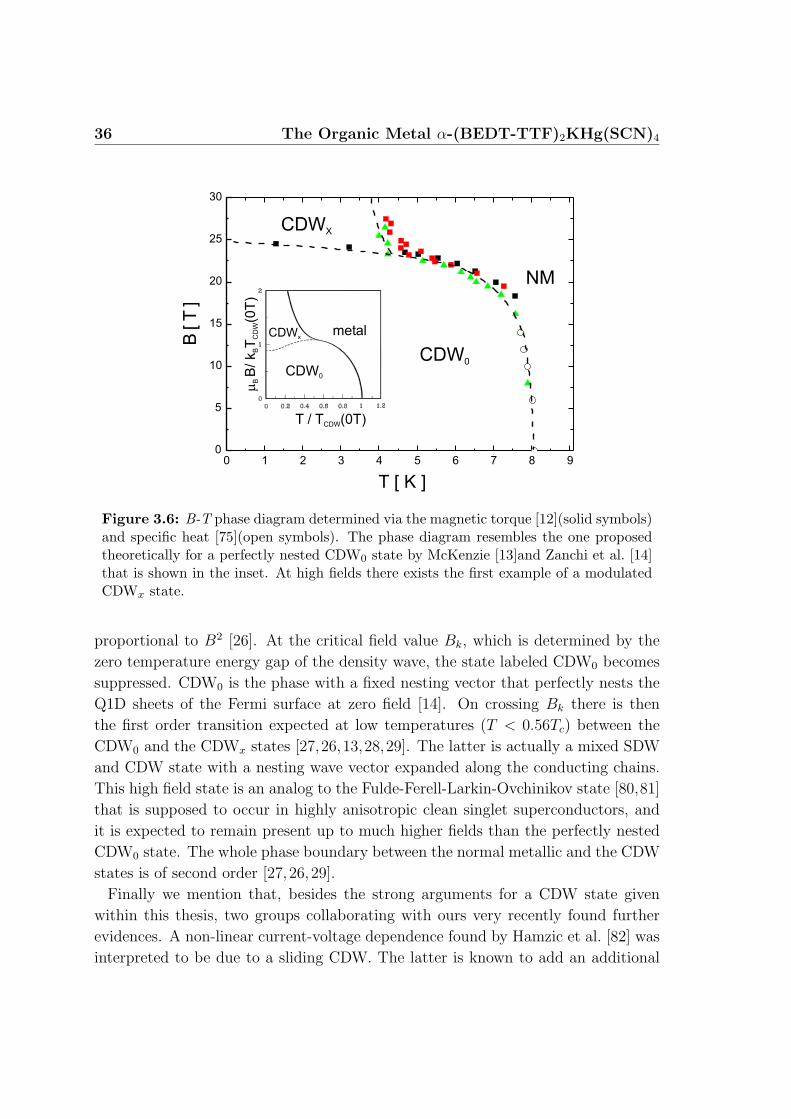
36 The Organic Metal α-(BEDT-TTF)2KHg(SCN)4
0 1 2 3 4 5 6 7 8 90
5
10
15
20
25
30
CDWX
NM
CDW0
B[T
]
T [ K ]
metal
CDW0
CDWx
T / T (0T)CDW
mB
BC
DW
B/ k
T(0
T)
Figure 3.6: B-T phase diagram determined via the magnetic torque [12](solid symbols)and specific heat [75](open symbols). The phase diagram resembles the one proposedtheoretically for a perfectly nested CDW0 state by McKenzie [13]and Zanchi et al. [14]that is shown in the inset. At high fields there exists the first example of a modulatedCDWx state.
proportional to B2 [26]. At the critical field value Bk, which is determined by the
zero temperature energy gap of the density wave, the state labeled CDW0 becomes
suppressed. CDW0 is the phase with a fixed nesting vector that perfectly nests the
Q1D sheets of the Fermi surface at zero field [14]. On crossing Bk there is then
the first order transition expected at low temperatures (T < 0.56Tc) between the
CDW0 and the CDWx states [27,26,13,28,29]. The latter is actually a mixed SDW
and CDW state with a nesting wave vector expanded along the conducting chains.
This high field state is an analog to the Fulde-Ferell-Larkin-Ovchinikov state [80,81]
that is supposed to occur in highly anisotropic clean singlet superconductors, and
it is expected to remain present up to much higher fields than the perfectly nested
CDW0 state. The whole phase boundary between the normal metallic and the CDW
states is of second order [27, 26,29].
Finally we mention that, besides the strong arguments for a CDW state given
within this thesis, two groups collaborating with ours very recently found further
evidences. A non-linear current-voltage dependence found by Hamzic et al. [82] was
interpreted to be due to a sliding CDW. The latter is known to add an additional
3.4 The Low Temperature Ground States 37
0 4 8 12 16 20 240
30
6026 T
0 T9 T
B:
T [ K ]
0 5 10 15 20 25 300
20
40
60
80
Bkink
T = 1.35 K
B [ T ]
R [
]W
R [
]W
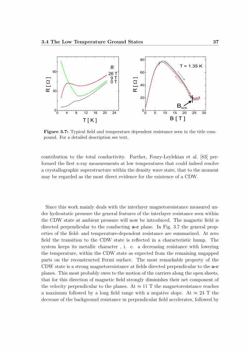
Figure 3.7: Typical field and temperature dependent resistance seen in the title com-pound. For a detailed description see text.
contribution to the total conductivity. Further, Foury-Leylekian et al. [83] per-
formed the first x-ray measurements at low temperatures that could indeed resolve
a crystallographic superstructure within the density wave state, that to the moment
may be regarded as the most direct evidence for the existence of a CDW.
Since this work mainly deals with the interlayer magnetoresistance measured un-
der hydrostatic pressure the general features of the interlayer resistance seen within
the CDW state at ambient pressure will now be introduced. The magnetic field is
directed perpendicular to the conducting a-c plane. In Fig. 3.7 the general prop-
erties of the field- and temperature-dependent resistance are summarized. At zero
field the transition to the CDW state is reflected in a characteristic hump. The
system keeps its metallic character , i. e. a decreasing resistance with lowering
the temperature, within the CDW state as expected from the remaining ungapped
parts on the reconstructed Fermi surface. The most remarkable property of the
CDW state is a strong magnetoresistance at fields directed perpendicular to the a-c
planes. This most probably owes to the motion of the carriers along the open sheets,
that for this direction of magnetic field strongly diminishes their net component of
the velocity perpendicular to the planes. At ≈ 11 T the magnetoresistance reaches
a maximum followed by a long field range with a negative slope. At ≈ 24 T the
decrease of the background resistance in perpendicular field accelerates, followed by
38 The Organic Metal α-(BEDT-TTF)2KHg(SCN)4
Q2D AMRO
Q1D AMRO
Q1D AMRO
Q2D AMROj
j
angle (degrees)q
inte
rlayer
resis
tance (
arb
. units )
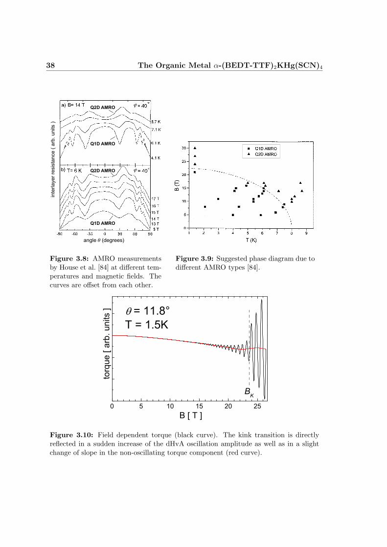
Figure 3.8: AMRO measurementsby House et al. [84] at different tem-peratures and magnetic fields. Thecurves are offset from each other.
Figure 3.9: Suggested phase diagram due todifferent AMRO types [84].
Figure 3.10: Field dependent torque (black curve). The kink transition is directlyreflected in a sudden increase of the dHvA oscillation amplitude as well as in a slightchange of slope in the non-oscillating torque component (red curve).
3.5 Effects of Hydrostatic Pressure 39
a moderate increase that determines the so-called ”kink”-transition from the CDW0
into the modulated CDWx state. Correspondingly, distinct changes can be seen in
the temperature sweeps of the magnetoresistance on entering both CDW states. On
sweeping the field up and down there is a hysteresis observed in a wide field range
within the CDW0 state, the origin being still unknown. The negative magnetoresis-
tance above 11 T is thought to occur due to magnetic breakdown between the open
trajectories and the small pockets [85], depicted in Fig. 3.5. This means that the
electrons again start to circle around the initial cylindrical part of the Fermi sur-
face. The decrease in the background magnetoresistance is thus related to a gradual
change of the AMROs from a Q1D to a Q2D character. In Fig. 3.8 results of House
et al. are shown [84]. They measured AMROs at different temperatures and fields
and could determine an approximate phase transition line separating Q1D AMRO
from the Q2D AMRO regions, see Fig. 3.9.
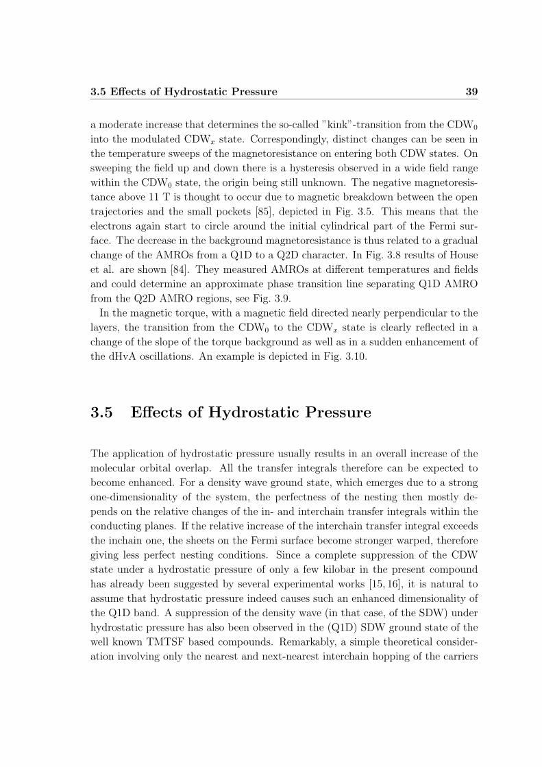
In the magnetic torque, with a magnetic field directed nearly perpendicular to the
layers, the transition from the CDW0 to the CDWx state is clearly reflected in a
change of the slope of the torque background as well as in a sudden enhancement of
the dHvA oscillations. An example is depicted in Fig. 3.10.
3.5 Effects of Hydrostatic Pressure
The application of hydrostatic pressure usually results in an overall increase of the
molecular orbital overlap. All the transfer integrals therefore can be expected to
become enhanced. For a density wave ground state, which emerges due to a strong
one-dimensionality of the system, the perfectness of the nesting then mostly de-
pends on the relative changes of the in- and interchain transfer integrals within the
conducting planes. If the relative increase of the interchain transfer integral exceeds
the inchain one, the sheets on the Fermi surface become stronger warped, therefore
giving less perfect nesting conditions. Since a complete suppression of the CDW
state under a hydrostatic pressure of only a few kilobar in the present compound
has already been suggested by several experimental works [15, 16], it is natural to
assume that hydrostatic pressure indeed causes such an enhanced dimensionality of
the Q1D band. A suppression of the density wave (in that case, of the SDW) under
hydrostatic pressure has also been observed in the (Q1D) SDW ground state of the
well known TMTSF based compounds. Remarkably, a simple theoretical consider-
ation involving only the nearest and next-nearest interchain hopping of the carriers
40 The Organic Metal α-(BEDT-TTF)2KHg(SCN)4
turned out to describe the experimental observations on the SDW under hydrostatic
pressure very well [2]. Since a similar theoretical consideration exists for a (Q1D)
CDW system in an applied magnetic field [14], a direct comparison of our experi-
mental results with theoretical predictions will be possible. As pointed out in the
theoretical background above, one can expect orbital effects of the charge carriers
to become important on worsening the nesting conditions of the CDW system.
Concerning the superconducting state existing in many BEDT-TTF based salts,
the anisotropy of the electron system also seems to be important. Generally, these
superconductors turn out to possess a very strong pressure dependence of the transi-
tion temperature, Tc, that amounts to the order of -1 K/kbar. Since Tc was suggested
to correlate with the anion layer thickness [9], its strong pressure dependence might
be attributed to the strong interlayer compressibility. On the contrary Q1D organic
superconductors do show a much weaker pressure dependence of Tc of about an
order of magnitude lower. Here the strong lattice stiffening rather than the above
lattice pressure effect is thought to be the reason. This means that the change
in the phonon spectrum, as for conventional superconductors, leads to a reduced
electron-phonon coupling that finally leads to a decrease of Tc.
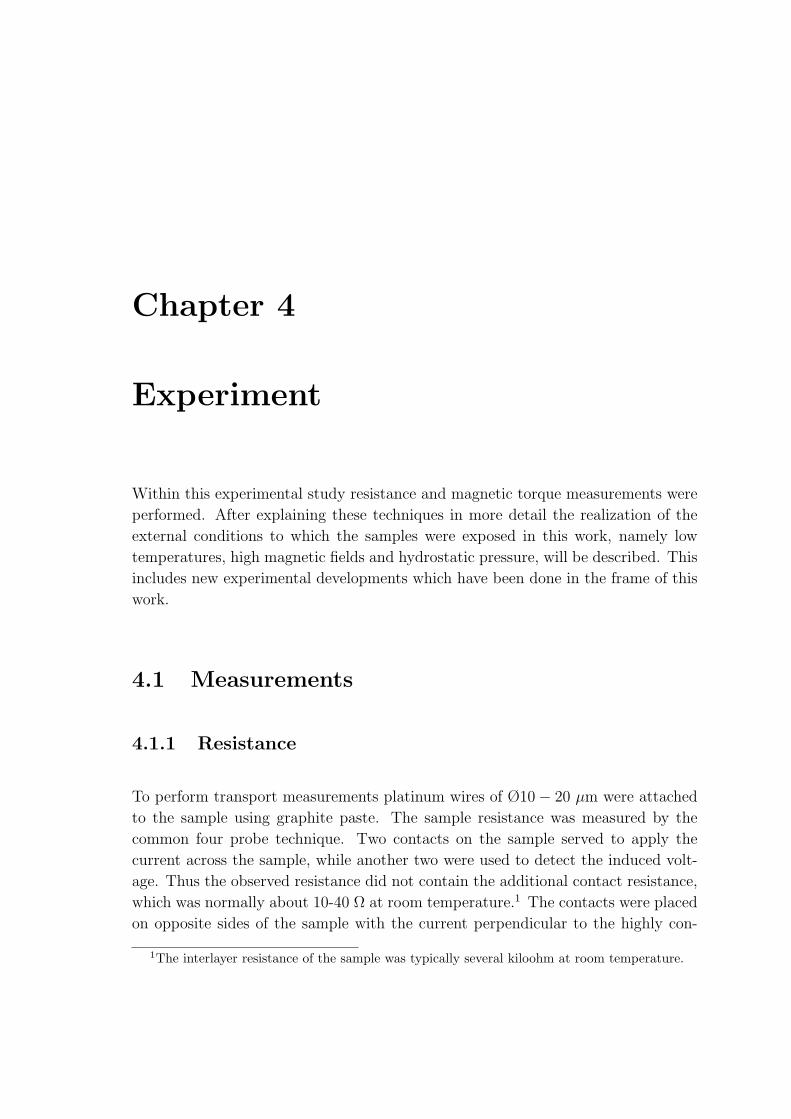
Chapter 4
Experiment
Within this experimental study resistance and magnetic torque measurements were
performed. After explaining these techniques in more detail the realization of the
external conditions to which the samples were exposed in this work, namely low
temperatures, high magnetic fields and hydrostatic pressure, will be described. This
includes new experimental developments which have been done in the frame of this
work.
4.1 Measurements
4.1.1 Resistance
To perform transport measurements platinum wires of Ø10− 20 µm were attached
to the sample using graphite paste. The sample resistance was measured by the
common four probe technique. Two contacts on the sample served to apply the
current across the sample, while another two were used to detect the induced volt-
age. Thus the observed resistance did not contain the additional contact resistance,
which was normally about 10-40 Ω at room temperature.1 The contacts were placed
on opposite sides of the sample with the current perpendicular to the highly con-
1The interlayer resistance of the sample was typically several kiloohm at room temperature.
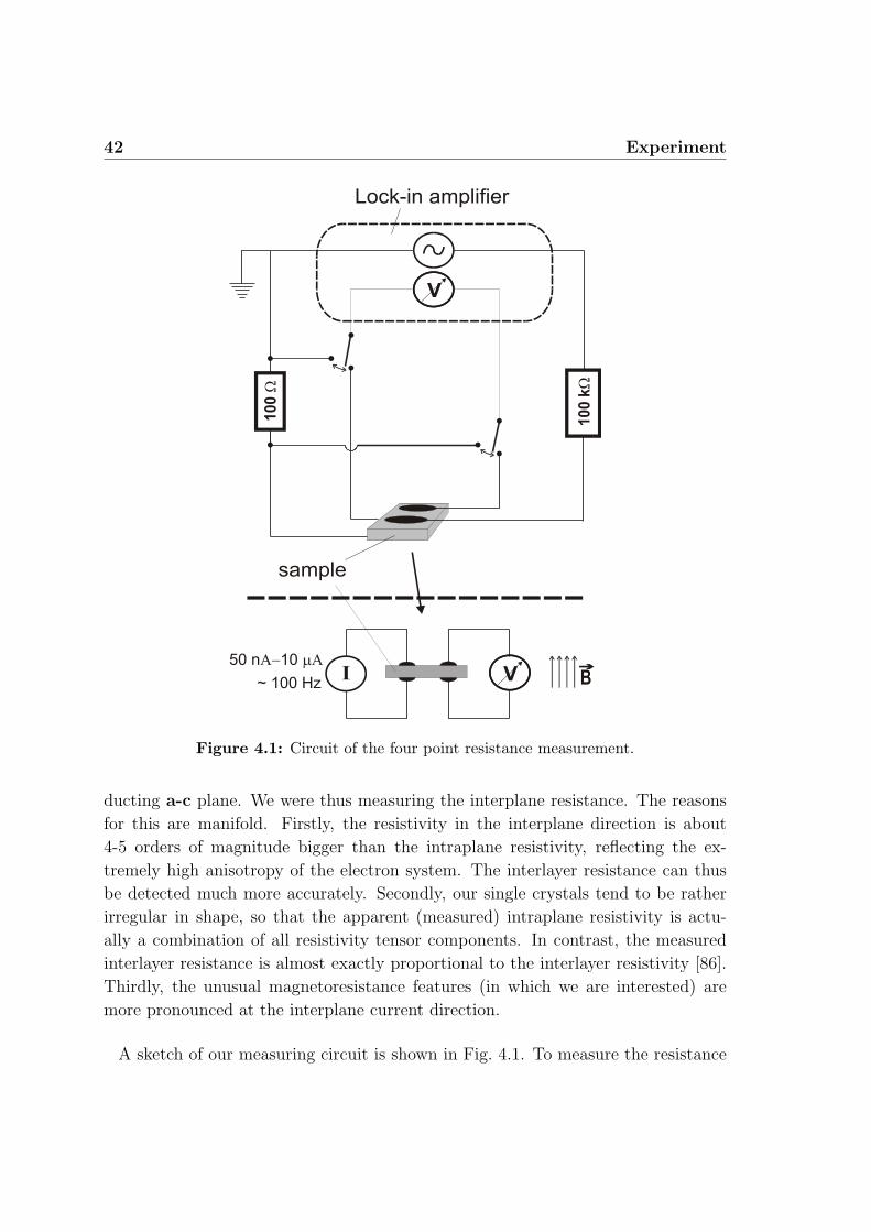
42 Experiment
~ 100 Hz
50 nA-10 mA
Figure 4.1: Circuit of the four point resistance measurement.
ducting a-c plane. We were thus measuring the interplane resistance. The reasons
for this are manifold. Firstly, the resistivity in the interplane direction is about
4-5 orders of magnitude bigger than the intraplane resistivity, reflecting the ex-
tremely high anisotropy of the electron system. The interlayer resistance can thus
be detected much more accurately. Secondly, our single crystals tend to be rather
irregular in shape, so that the apparent (measured) intraplane resistivity is actu-
ally a combination of all resistivity tensor components. In contrast, the measured
interlayer resistance is almost exactly proportional to the interlayer resistivity [86].
Thirdly, the unusual magnetoresistance features (in which we are interested) are
more pronounced at the interplane current direction.
A sketch of our measuring circuit is shown in Fig. 4.1. To measure the resistance
4.1 Measurements 43
an AC current of 0.01 to 10 µA with a frequency of the order of 100 Hz is applied
and the voltage is amplified and detected by a highly sensitive lock-in amplifier. The
low current value serves to prevent overheating of the sample at low temperatures,
and has to be adjusted to the given experimental conditions, e.g. contact resistances
and temperature range. To keep the current amplitude constant and stable during
the measurement a high resistance (typically 100 kΩ- 1 MΩ) is placed in series. For
the adjustment of the current and the phase a reference resistance (of 10-100 Ω) is
placed into the circuit. By measuring the AC voltage across this resistance a desired
current value can be set.
The absolute sample resistance at low temperatures (with or without a magnetic
field) was thus checked to be detected to an accuracy of at least 5 %. The signal-
to-noise ratio during our measurements was typically & 104.
4.1.2 Magnetic Torque
A magnetic moment m placed into an external magnetic field H experiences a torque
τ in the direction perpendicular to m and H:
τ = m×B, (4.1)
where B is the magnetic induction in the sample, B = µµ0H. In our compounds we
assume µ ≈ 1.2 For a sample with a homogeneous magnetization M over its volume
V the torque then amounts to:
τ = M⊥BV, (4.2)
where M⊥ is the component perpendicular to the field direction. For the measure-
ment of quantum oscillations, using Eq. (2.19) the oscillatory torque may thus be
written in terms of the magnetization M‖ parallel to the field:
τ = − 1
F
∂F
∂θM‖BV. (4.3)
The detection of the dHvA oscillations by the torque method obviously needs an
anisotropic Fermi surface, ∂F∂θ6= 0. Further, the torque vanishes if the magnetic
field is directed along a symmetry axis of the crystal. In such cases either ∂F∂θ
= 0
or opposite components of the torque cancel each other out. This offers a perfect
possibility to align the sample or, in other words, calibrate the offset angle with
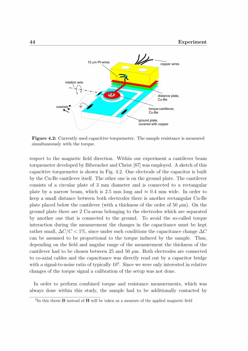
44 Experiment
coaxials
10 m Pt-wiresm
distance plate,Cu-Be
torque-cantilever,Cu-Be
copper wires
ground plate,covered with copper
rotation axis
Figure 4.2: Currently used capacitive torquemeter. The sample resistance is measuredsimultaneously with the torque.
respect to the magnetic field direction. Within our experiment a cantilever beam
torquemeter developed by Biberacher and Christ [87] was employed. A sketch of this
capacitive torquemeter is shown in Fig. 4.2. One electrode of the capacitor is built
by the Cu-Be cantilever itself. The other one is on the ground plate. The cantilever
consists of a circular plate of 3 mm diameter and is connected to a rectangular
plate by a narrow beam, which is 2.5 mm long and ≈ 0.4 mm wide. In order to
keep a small distance between both electrodes there is another rectangular Cu-Be
plate placed below the cantilever (with a thickness of the order of 50 µm). On the
ground plate there are 2 Cu-areas belonging to the electrodes which are separated
by another one that is connected to the ground. To avoid the so-called torque
interaction during the measurement the changes in the capacitance must be kept
rather small, ∆C/C < 1%, since under such conditions the capacitance change ∆C
can be assumed to be proportional to the torque induced by the sample. Thus,
depending on the field and angular range of the measurement the thickness of the
cantilever had to be chosen between 25 and 50 µm. Both electrodes are connected
to co-axial cables and the capacitance was directly read out by a capacitor bridge
with a signal-to-noise ratio of typically 105. Since we were only interested in relative
changes of the torque signal a calibration of the setup was not done.
In order to perform combined torque and resistance measurements, which was
always done within this study, the sample had to be additionally contacted by
2In this thesis B instead of H will be taken as a measure of the applied magnetic field
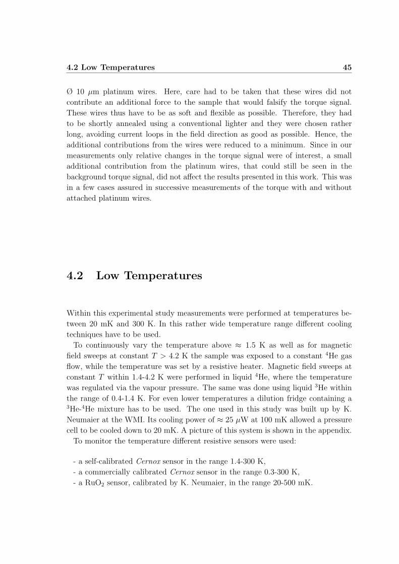
4.2 Low Temperatures 45
Ø 10 µm platinum wires. Here, care had to be taken that these wires did not
contribute an additional force to the sample that would falsify the torque signal.
These wires thus have to be as soft and flexible as possible. Therefore, they had
to be shortly annealed using a conventional lighter and they were chosen rather
long, avoiding current loops in the field direction as good as possible. Hence, the
additional contributions from the wires were reduced to a minimum. Since in our
measurements only relative changes in the torque signal were of interest, a small
additional contribution from the platinum wires, that could still be seen in the
background torque signal, did not affect the results presented in this work. This was
in a few cases assured in successive measurements of the torque with and without
attached platinum wires.
4.2 Low Temperatures
Within this experimental study measurements were performed at temperatures be-
tween 20 mK and 300 K. In this rather wide temperature range different cooling
techniques have to be used.
To continuously vary the temperature above ≈ 1.5 K as well as for magnetic
field sweeps at constant T > 4.2 K the sample was exposed to a constant 4He gas
flow, while the temperature was set by a resistive heater. Magnetic field sweeps at
constant T within 1.4-4.2 K were performed in liquid 4He, where the temperature
was regulated via the vapour pressure. The same was done using liquid 3He within
the range of 0.4-1.4 K. For even lower temperatures a dilution fridge containing a3He-4He mixture has to be used. The one used in this study was built up by K.
Neumaier at the WMI. Its cooling power of ≈ 25 µW at 100 mK allowed a pressure
cell to be cooled down to 20 mK. A picture of this system is shown in the appendix.
To monitor the temperature different resistive sensors were used:
- a self-calibrated Cernox sensor in the range 1.4-300 K,
- a commercially calibrated Cernox sensor in the range 0.3-300 K,
- a RuO2 sensor, calibrated by K. Neumaier, in the range 20-500 mK.
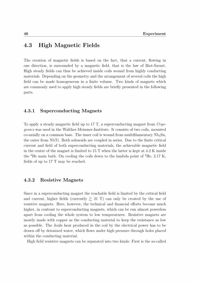
46 Experiment
4.3 High Magnetic Fields
The creation of magnetic fields is based on the fact, that a current, flowing in
one direction, is surrounded by a magnetic field, that is the law of Biot-Savart.
High steady fields can thus be achieved inside coils wound from highly conducting
materials. Depending on the geometry and the arrangement of several coils the high
field can be made homogeneous in a finite volume. Two kinds of magnets which
are commonly used to apply high steady fields are briefly presented in the following
parts.
4.3.1 Superconducting Magnets
To apply a steady magnetic field up to 17 T, a superconducting magnet from Cryo-
genics was used in the Walther-Meissner-Institute. It consists of two coils, mounted
co-axially on a common base. The inner coil is wound from multifilamentary Nb3Sn,
the outer from NbTi. Both solenoids are coupled in series. Due to the finite critical
current and field of both superconducting materials, the achievable magnetic field
in the centre of the magnet is limited to 15 T when the latter is kept at 4.2 K inside
the 4He main bath. On cooling the coils down to the lambda point of 4He, 2.17 K,
fields of up to 17 T may be reached.
4.3.2 Resistive Magnets
Since in a superconducting magnet the reachable field is limited by the critical field
and current, higher fields (currently & 21 T) can only be created by the use of
resistive magnets. Here, however, the technical and financial efforts become much
higher, in contrast to superconducting magnets, which can be run almost powerless
apart from cooling the whole system to low temperatures. Resistive magnets are
mostly made with copper as the conducting material to keep the resistance as low
as possible. The Joule heat produced in the coil by the electrical power has to be
drawn off by deionized water, which flows under high pressure through holes placed
within the conducting material.
High field resistive magnets can be separated into two kinds: First is the so-called
4.3 High Magnetic Fields 47
Bittermagnets
polyhelixmagnets
coolingwater
out
in
bore 50 mm
Figure 4.3: Sketch of a 30 Tesla magnet used in the high field lab in Grenoble.
Bitter magnet (named after the inventor). Copper discs are layered on each other
with an insulating material in between except a slice of about 20. By pressing them
together with a strong force a sort of coil is built with a radial current density that
is inversely proportional to the distance from the coil axis. To prevent the system
from ”melting”, deionized water flows through holes, drilled parallel to the coil axis
through the copper discs.
Another resistive magnet is the polyhelix magnet. It consists of several copper
coils fitted coaxially into each other. The advantage in comparison to the Bitter
magnet is, that the current density can be regulated radial to the field. In this work
48 Experiment
high field (> 17 T) experiments were made in the High Magnetic Field Laboratory
(HMFL) in Grenoble with a resistive magnet. Here, two Bitter magnets are placed
around a polyhelix magnet, Fig. 4.3. This configuration allows to reach a maximum
steady field of 30 T at a current of 10 kA and a water flow of 1000 m3/h, while
applying the power of 20 MW.
4.4 Hydrostatic Pressure
In this work two different pressure techniques have been applied, one using helium
and the other silicon oil as a pressure medium. Since the former technique was
further tested and improved for the use at low temperatures in the frame of this
work, this will be described in more detail.
4.4.1 4He-pressure Apparatus
In Fig. 4.4 the whole 4He pressure setup is sketched. It can be roughly separated
into two stages. One, where the pressure never exceeds 3 kbar and another, where
pressures up to 10 kbar (= 1 GPa) can be reached. 4He comes from the gas bottle
(P=180 bar) into the completely pumped system and is filtered in a nitrogen trap.
This prevents blockages in the lines during pressurisation, especially at low temper-
atures inside the cryostat. In the first stage, a membrane compressor applies up to
3 kbar to the whole pressure system. After the desired pressure is reached the valve
between the first and second stage is closed. Oil pressure then drives up a piston in
an amplifier that reduces the volume of the second stage. The pressure applied from
the first stage can thus be multiplied by a factor of 4. The high pressure is then
transferred via a 4 m long Cu-Be capillary to the pressure cell inside the cryostat.
Except this low-temperature part, all parts of the system were bought from the
company ”Nova Swiss”. To monitor the pressure, commercial (membrane) pressure
sensors are placed in each stage, one measuring up to 3 kbar and another up to
10 kbar. In order to prevent damages of the compressor and the pressure sensor in
the first stage, a rupture disk is located there which would immediately break if the
pressure exceeds 3 kbar. For safety reasons, in the case of an explosive decompres-
sion of the system, a steel rope is fixed to the Cu-Be tube and the whole system is
surrounded with thick plastic shields. The pressure system was successfully tested
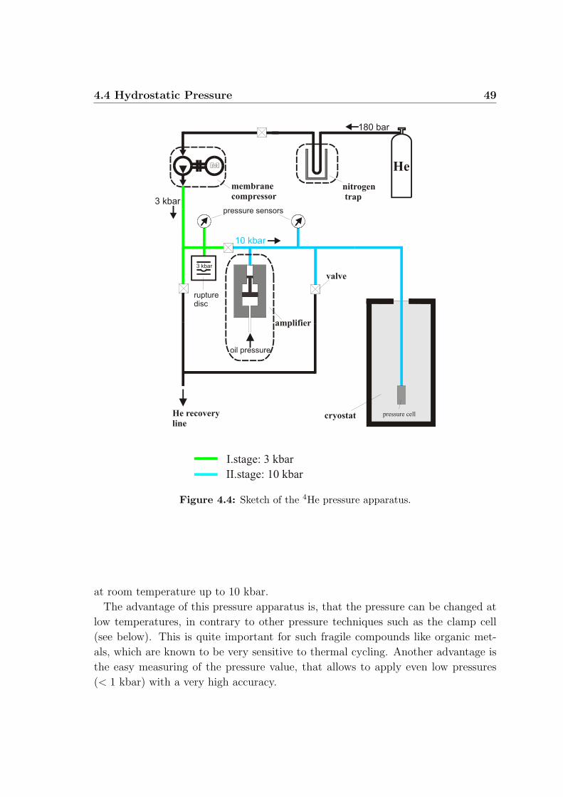
4.4 Hydrostatic Pressure 49
pressure cell
membranecompressor
nitrogentrap
amplifier
cryostat
oil pressure
180 bar
3 kbar
10 kbar
He recoveryline
He
pressure sensors
valve
3 kbar
rupturedisc
I.stage: 3 kbar
II.stage: 10 kbar
Figure 4.4: Sketch of the 4He pressure apparatus.
at room temperature up to 10 kbar.
The advantage of this pressure apparatus is, that the pressure can be changed at
low temperatures, in contrary to other pressure techniques such as the clamp cell
(see below). This is quite important for such fragile compounds like organic met-
als, which are known to be very sensitive to thermal cycling. Another advantage is
the easy measuring of the pressure value, that allows to apply even low pressures
(< 1 kbar) with a very high accuracy.
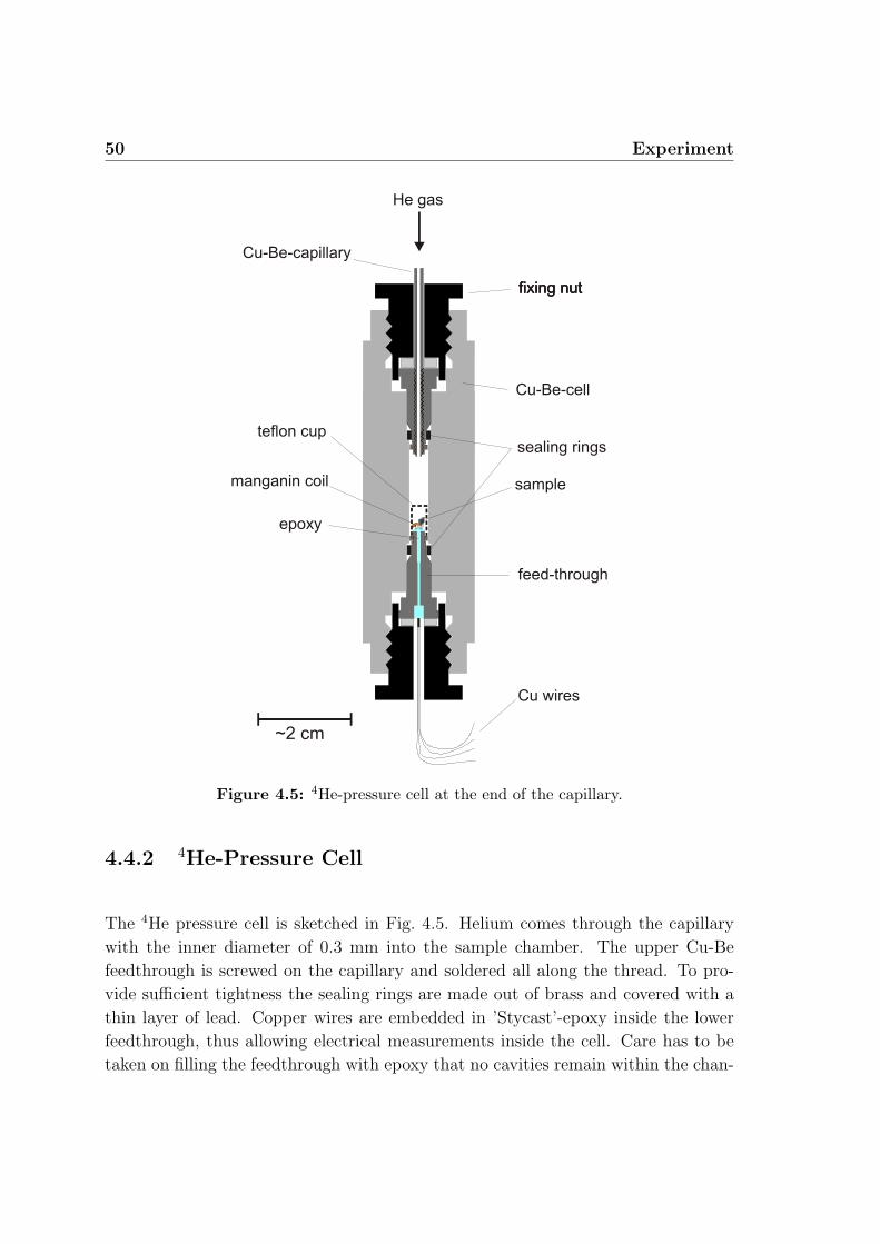
50 Experiment
Cu- -cellBe
sealing rings
fixing nut
feed-through
sample
fixing nutfixing nut
Cu- -capillaryBe
manganin coil
teflon cup
He gas
Cu wires
~2 cm
Figure 4.5: 4He-pressure cell at the end of the capillary.
4.4.2 4He-Pressure Cell
The 4He pressure cell is sketched in Fig. 4.5. Helium comes through the capillary
with the inner diameter of 0.3 mm into the sample chamber. The upper Cu-Be
feedthrough is screwed on the capillary and soldered all along the thread. To pro-
vide sufficient tightness the sealing rings are made out of brass and covered with a
thin layer of lead. Copper wires are embedded in ’Stycast’-epoxy inside the lower
feedthrough, thus allowing electrical measurements inside the cell. Care has to be
taken on filling the feedthrough with epoxy that no cavities remain within the chan-
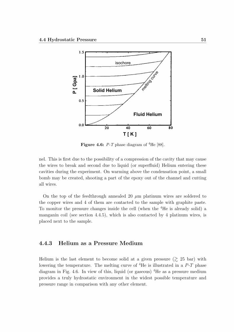
4.4 Hydrostatic Pressure 51
Fluid Helium
Solid Helium mel
ting
curv
e
isochore
P[
Gp
a]
T [ K ]
Figure 4.6: P-T phase diagram of 4He [88].
nel. This is first due to the possibility of a compression of the cavity that may cause
the wires to break and second due to liquid (or superfluid) Helium entering these
cavities during the experiment. On warming above the condensation point, a small
bomb may be created, shooting a part of the epoxy out of the channel and cutting
all wires.
On the top of the feedthrough annealed 20 µm platinum wires are soldered to
the copper wires and 4 of them are contacted to the sample with graphite paste.
To monitor the pressure changes inside the cell (when the 4He is already solid) a
manganin coil (see section 4.4.5), which is also contacted by 4 platinum wires, is
placed next to the sample.
4.4.3 Helium as a Pressure Medium
Helium is the last element to become solid at a given pressure (& 25 bar) with
lowering the temperature. The melting curve of 4He is illustrated in a P -T phase
diagram in Fig. 4.6. In view of this, liquid (or gaseous) 4He as a pressure medium
provides a truly hydrostatic environment in the widest possible temperature and
pressure range in comparison with any other element.
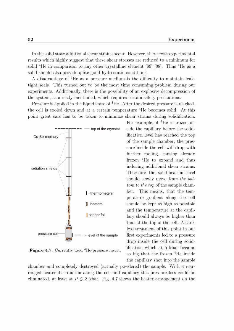
52 Experiment
In the solid state additional shear strains occur. However, there exist experimental
results which highly suggest that these shear stresses are reduced to a minimum for
solid 4He in comparison to any other crystalline element [89] [88]. Thus 4He as a
solid should also provide quite good hydrostatic conditions.
A disadvantage of 4He as a pressure medium is the difficulty to maintain leak-
tight seals. This turned out to be the most time consuming problem during our
experiments. Additionally, there is the possibility of an explosive decompression of
the system, as already mentioned, which requires certain safety precautions.
Pressure is applied in the liquid state of 4He. After the desired pressure is reached,
the cell is cooled down and at a certain temperature 4He becomes solid. At this
point great care has to be taken to minimize shear strains during solidification.
thermometers
pressure cell
radiation shields
Cu-Be-capillary
top of the cryostat
~ level of the sample
copper foil
Figure 4.7: Currently used 4He-pressure insert.
For example, if 4He is frozen in-
side the capillary before the solid-
ification level has reached the top
of the sample chamber, the pres-
sure inside the cell will drop with
further cooling, causing already
frozen 4He to expand and thus
inducing additional shear strains.
Therefore the solidification level
should slowly move from the bot-
tom to the top of the sample cham-
ber. This means, that the tem-
perature gradient along the cell
should be kept as high as possible
and the temperature at the capil-
lary should always be higher than
that at the top of the cell. A care-
less treatment of this point in our
first experiments led to a pressure
drop inside the cell during solid-
ification which at 5 kbar became
so big that the frozen 4He inside
the capillary shot into the sample
chamber and completely destroyed (actually powdered) the sample. With a rear-
ranged heater distribution along the cell and capillary this pressure loss could be
eliminated, at least at P . 3 kbar. Fig. 4.7 shows the heater arrangement on the
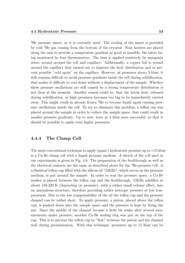
4.4 Hydrostatic Pressure 53
4He pressure insert, as it is currently used. The cooling of the insert is provided
by cold 4He gas coming from the bottom of the cryostat. Four heaters are placed
along the axis to provide a temperature gradient as good as possible, the latter be-
ing monitored by four thermometers. The heat is applied resistively by manganin
wires, wound around the cell and capillary. Additionally, a copper foil is wound
around the capillary that turned out to improve the heat distribution and to pre-
vent possible ”cold spots” on the capillary. However, at pressures above 3 kbar, it
still remains difficult to avoid pressure gradients inside the cell during solidification,
that makes it difficult to cool down without a displacement of the sample. Whether
these pressure oscillations are still caused by a wrong temperature distribution is
not clear at the moment. Another reason could be, that the latent heat, released
during solidification, at high pressures becomes too big to be immediately carried
away. This might result in already frozen 4He to become liquid again causing pres-
sure oscillations inside the cell. To try to eliminate this problem, a teflon cup was
placed around the sample in order to reduce the sample space, that could result in
smaller pressure gradients. Up to now, tests at 4 kbar were successful, so that it
should be possible to apply even higher pressures.
4.4.4 The Clamp Cell
The most conventional technique to apply (quasi-) hydrostatic pressure up to ∼15 kbar
is a Cu-Be clamp cell with a liquid pressure medium. A sketch of the cell used in
our experiments is given in Fig. 4.8. The preparation of the feedthrough as well as
the electrical contacts are the same as described above for the 4He-pressure cell. A
cylindrical teflon cup filled with the silicon oil ”GKZh”, which serves as the pressure
medium, is put around the sample. In order to seal the pressure space, a Cu-Be
washer is placed between the teflon cup and the feedthrough. GKZh solidifies at
about 150-220 K (depending on pressure), with a rather small volume effect, into
an amorphous structure, therefore providing rather isotropic pressure at low tem-
peratures. Due to the low compressibility of the oil the teflon cup and the pressure
channel can be rather short. To apply pressure, a piston, placed above the teflon
cup, is pushed down into the sample space and the pressure is kept by fixing the
nut. Since the middle of the channel became a little bit wider after several mea-
surements under pressure, another Cu-Be sealing ring was put on the top of the
cup. This is to prevent the teflon cup to ”flow” between the piston and the channel
wall during pressurisation. With this technique, pressures up to 15 kbar can be
54 Experiment
Cu wiresnut
“mushroom”
nut
piston
feedthroughepoxy
Pt-wiressample + coil
teflon cup
Cu- -washerBe
Cu- -cellBe
~ 10 mm
Figure 4.8: The liquid medium clamp cell.
applied without a problem. To measure the pressure, a manganin coil, calibrated
with the 4He pressure station, was placed next to the sample. To cool a pressurized
sample down to the lowest possible temperature the cell has been mounted on a
dilution refrigerator. Here, problems appeared on applying high magnetic fields.
Besides the expected eddy current heating, while sweeping the field, the cell showed
a considerable demagnetization effect on ramping the field down. The latter cool-
ing mechanism could be reduced with a new cell that was made out of very pure
Cu-Be containing less magnetic impurities. However, these two parasitic effects
made it impossible to make magnetic field sweeps (in the tesla range) and especially
to study the hysteretic magnetoresistance between raising and falling fields below
T = 100 mK.
4.4.5 Pressure Determination
The pressure inside both cells (described above), was monitored by a manganin coil.
It was wound from a 50 µm manganin wire and the coil resistance took the value of
a few Ω. The resistance of manganin is known to depend linearly on pressure. For a
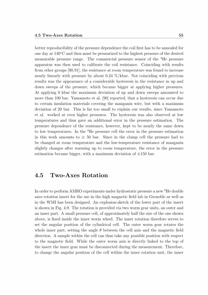
4.5 Two-Axes Rotation 55
better reproducibility of the pressure dependence the coil first has to be annealed for
one day at 140C and then must be pressurized to the highest pressure of the desired
measurable pressure range. The commercial pressure sensor of the 4He pressure
apparatus was then used to calibrate the coil resistance. Coinciding with results
from other groups [90,91], the resistance at room temperature was found to increase
nearly linearly with pressure by about 0.24 %/kbar. Not coinciding with previous
results was the appearance of a considerable hysteresis in the resistance in up and
down sweeps of the pressure, which became bigger at applying higher pressures.
At applying 8 kbar the maximum deviation of up and down sweeps amounted to
more than 100 bar. Yamamoto et al. [90] reported, that a hysteresis can occur due
to certain insulation materials covering the manganin wire, but with a maximum
deviation of 20 bar. This is far too small to explain our results, since Yamamoto
et al. worked at even higher pressures. The hysteresis was also observed at low
temperatures and thus gave an additional error in the pressure estimation. The
pressure dependence of the resistance, however, kept to be nearly the same down
to low temperatures. In the 4He pressure cell the error in the pressure estimation
in this work amounts to ± 50 bar. Since in the clamp cell the pressure had to
be changed at room temperature and the low-temperature resistance of manganin
slightly changes after warming up to room temperature, the error in the pressure
estimation became bigger, with a maximum deviation of ±150 bar.
4.5 Two-Axes Rotation
In order to perform AMRO experiments under hydrostatic pressure a new 3He double
axes rotation insert for the use in the high magnetic field lab in Grenoble as well as
in the WMI has been designed. An explosion-sketch of the lower part of the insert
is shown in Fig. 4.9. The rotation is provided via two worm gear units, an outer and
an inner part. A small pressure cell, of approximately half the size of the one shown
above, is fixed inside the inner worm wheel. The inner rotation therefore serves to
set the angular position of the cylindrical cell. The outer worm gear rotates the
whole inner part, setting the angle θ between the cell axis and the magnetic field
direction. A sample within the cell can thus take any possible position with respect
to the magnetic field. While the outer worm axis is directly linked to the top of
the insert the inner gear must be disconnected during the measurement. Therefore,
to change the angular position of the cell within the inner rotation unit, the inner
56 Experiment
outergear wheeldrive
teflon cupteflon cup
outer gear wheel
inner gear wheel
inner gear wheeldrive
pressure cellholder
~10 mm
screwdriver
Figure 4.9: Self designed in-situ two-axes rotation unit allowing a small pressure cellto take any position with respect to the magnetic field.
worm axis has to be put to the vertical direction (by changing the angle θ) and a
screwdriver, that can be pushed down, has to ”catch” the slit on top of the inner
worm drive. Thus, by putting a sample inside the pressure cell with the interlayer
direction parallel to the cell axis this rotation unit is very suitable to perform AMRO
measurements. To diminish the heat production during the steady rotation of the
outer gear, the metal to metal friction on the suspension points is avoided by the
use of additional teflon cups placed in between. All the other parts in Fig. 4.9 are
made out of brass. The accuracy to which both angles can be set with this setup
amounts to < 0.05.
Since the whole insert is designed for the use in 30 T magnets, which possess
enormous stray fields, it is clear that the use of any kind of magnetic material is not
very suggestive. Therefore the driving force on the azimuthal rotation axis is given
by a piezo-electric motor. Due to a limited speed range of the latter an additional
gear is placed on the top of the insert. The gear reduction can be set over three
4.6 Sample Preparation and Treatment 57
orders of magnitude to 10 different values. The sweeping rate of the sample rotation
can thus be continuously changed in a wide range of ≈ 0.003 − 10/sec. Since a
steady rotation of the sample always causes heat induced by the friction, there will
be a low temperature limit depending on the rotation speed. With this setup the
lowest achievable temperature at a reasonable3 sweeping rate of 0.1-0.15/sec turned
out to be 0.7 K.
4.6 Sample Preparation and Treatment
The typical dimensions of the samples amounted to about 0.5×0.5×0.1 mm3 with
a corresponding mass of ≈ 75 µg. As a matter of fact the samples appear to be
mostly as-grown bi-crystals. This, however, falsifies the measurements in magnetic
field, since we know that our measurements strongly depend on the exact field
orientation. Therefore most of the samples had to be ground in order to get perfect
single crystals. To do this, the samples were embedded into a (afterwards solvable)
glue, allowing a part of the sample to be ground off with a conventional disk-grinder.
This method of preparing single crystals has turned out to be quite successful, in that
the quality of the samples was found not to suffer. This can be seen, for example,
from the amplitudes of the quantum oscillations. Actually, this is rather surprising
since the fragile samples are otherwise known to be very sensitive to the light and
also to thermal cyclings due to the easy formation of micro-cracks. Organic metals
generally should be kept in the dark and the cooling and heating rates during our
measurements were always checked not to exceed 3 K/min.
3here, ”reasonable” is linked to the strongly limited magnet time in the high field lab in Greno-ble.
58 Experiment

Chapter 5
Results and Discussion
60 Results and Discussion
5.1 The CDW Ground State under Hydrostatic
Pressure
5.1.1 Zero-Field Transition
The transition from the normal metallic state to the density wave state at ambient
pressure is manifested in a characteristic hump in the zero-field resistance. Within
the density wave state the resistance keeps a metallic behaviour, i.e. it decreases
with lowering the temperature. On cooling down from room temperature the inter-
layer resistance of α-(BEDT-TTF)2KHG(SCN)4 thus shows a steady decrease. The
residual resistance ratio between 1.4 K and room temperature in our measurements
was typically in between 50-200. This value is commonly taken as a measure of the
sample quality; i.e. a higher ratio determines a higher quality.
In Fig. 5.1 we plot the interlayer resistance, measured on the same sample at
different hydrostatic pressures at zero magnetic field. In the normal metallic state
the resistivity shows a strong negative pressure dependence of 1ρ· ∂ρ
∂P≈ 10−3MPa−1.
This is about 2 orders of magnitude larger than observed in conventional metals
like e.g. copper. With increasing pressure the hump moves down in temperature,
becoming less pronounced and at 2.3 kbar no sign of the transition is seen any more.
Obviously, the density wave state becomes suppressed under hydrostatic pressure,
which coincides with the results from other groups [15,16]. As a characteristic den-
sity wave transition temperature Tp we take here a minimum in the derivative (see
inset and vertical lines in Fig. 5.1) since this point at ambient pressure coincides
best with specific heat measurements [75].
These observations under hydrostatic pressure are easily understood by consider-
ing the overlap of the molecular orbitals. With pressure the small overlap across
the layers increases rather strong so that an enhanced conductivity should be ex-
pected. Furthermore, the transfer integrals between the conducting chains within
the layer also do increase, the relative enhancement being very likely stronger than
in the in-chain direction. Altogether we thus expect the electron system, and in
particular the Q1D part of the Fermi surface, to become less anisotropic. This in
turn explains the suppression of the density wave state. In Fig. 5.2 we plot the tran-
sition temperatures extracted from Fig. 5.1 against pressure. The data is compared
with the results from Schegolev et al. [94] obtained on the Tl-salt of this family of

5.1 The CDW Ground State under Hydrostatic Pressure 61
Figure 5.1: Zero-field resistance measured at different pressures [92, 93]. The upperleft inset shows the enlarged low temperature part of the curves. The lower right insetshows the determination of the CDW transition temperature from a minimum seen inthe derivative. The extracted transition temperatures are marked by vertical lines. Theapparent increase of the resistance at ' 12 K and 900 bar is due to a slight pressuredrop within the cell during the solidification of 4He
organic conductors possessing a slightly higher density wave transition temperature
(Tp =9 K) at ambient pressure. Both compounds show similar results. In the K-salt
Tp at 1.6 kbar decreased to ≈ 65% of the ambient pressure value.
An interesting observation is shown in the upper left inset of Fig. 5.1. Within the
density wave state the resistance, at low temperatures, shows an inverse pressure
dependence. It increases with pressure. Together with the facts that (i) within the
normal metallic (NM) state the pressure dependence of the resistance seems to be
temperature independent and that (ii) the NM state at 2.3 kbar persists to lower
temperatures, we then conclude that the resistance within the density wave state is
lower than the expected one in the NM state would be at the same temperature.
A lower resistance, however, is normally associated either with an increase of the
number of charge carriers contributing to the current, or with a longer carrier life
time, i.e. lower scattering rate or with an increase of their velocity. Since a part of
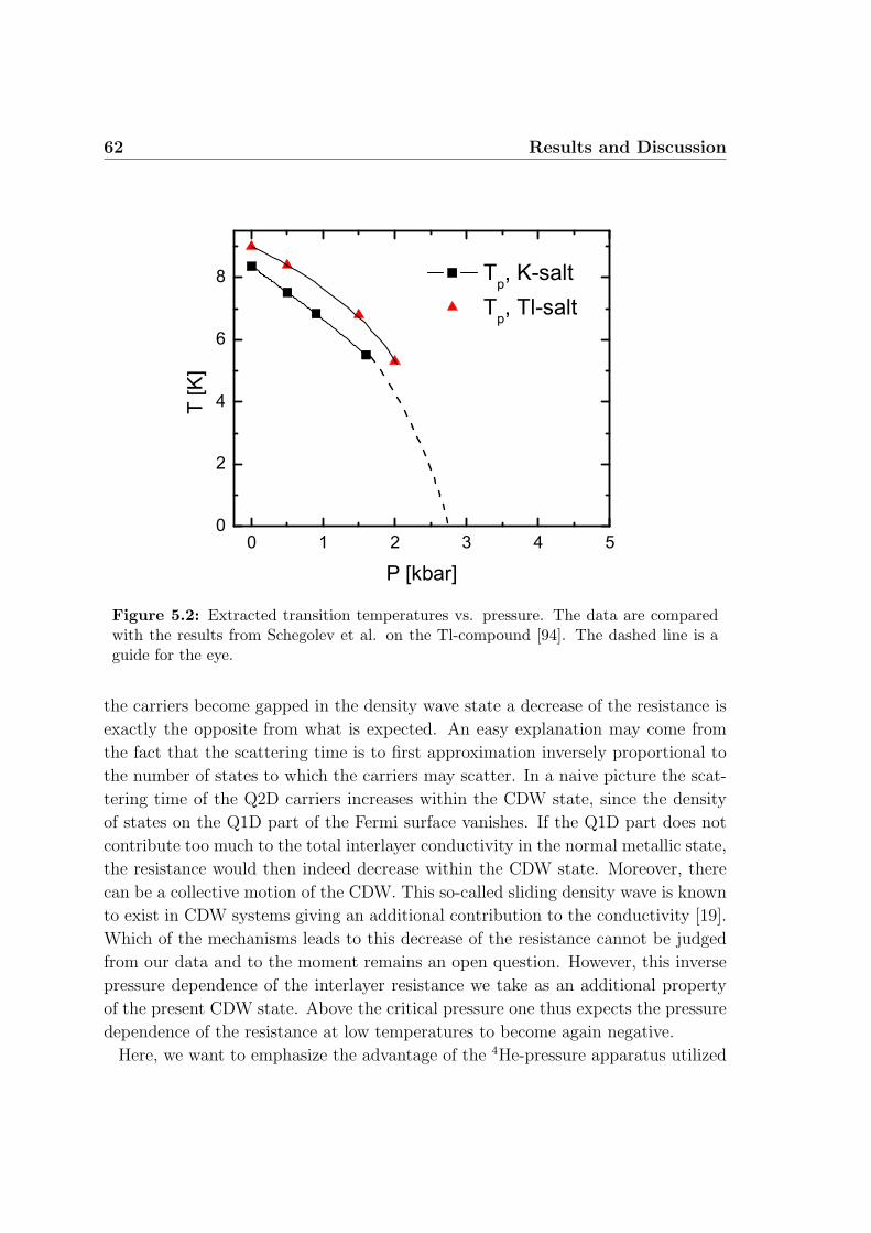
62 Results and Discussion
Figure 5.2: Extracted transition temperatures vs. pressure. The data are comparedwith the results from Schegolev et al. on the Tl-compound [94]. The dashed line is aguide for the eye.
the carriers become gapped in the density wave state a decrease of the resistance is
exactly the opposite from what is expected. An easy explanation may come from
the fact that the scattering time is to first approximation inversely proportional to
the number of states to which the carriers may scatter. In a naive picture the scat-
tering time of the Q2D carriers increases within the CDW state, since the density
of states on the Q1D part of the Fermi surface vanishes. If the Q1D part does not
contribute too much to the total interlayer conductivity in the normal metallic state,
the resistance would then indeed decrease within the CDW state. Moreover, there
can be a collective motion of the CDW. This so-called sliding density wave is known
to exist in CDW systems giving an additional contribution to the conductivity [19].
Which of the mechanisms leads to this decrease of the resistance cannot be judged
from our data and to the moment remains an open question. However, this inverse
pressure dependence of the interlayer resistance we take as an additional property
of the present CDW state. Above the critical pressure one thus expects the pressure
dependence of the resistance at low temperatures to become again negative.
Here, we want to emphasize the advantage of the 4He-pressure apparatus utilized
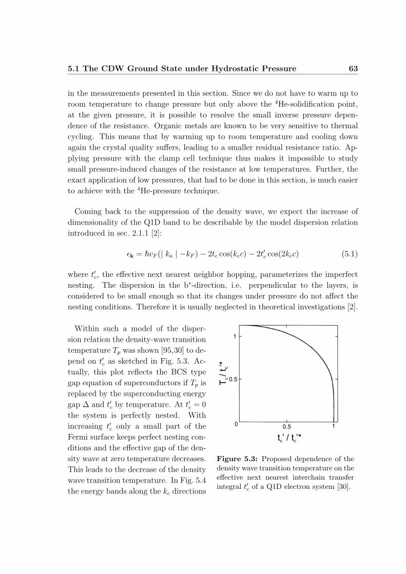
5.1 The CDW Ground State under Hydrostatic Pressure 63
in the measurements presented in this section. Since we do not have to warm up to
room temperature to change pressure but only above the 4He-solidification point,
at the given pressure, it is possible to resolve the small inverse pressure depen-
dence of the resistance. Organic metals are known to be very sensitive to thermal
cycling. This means that by warming up to room temperature and cooling down
again the crystal quality suffers, leading to a smaller residual resistance ratio. Ap-
plying pressure with the clamp cell technique thus makes it impossible to study
small pressure-induced changes of the resistance at low temperatures. Further, the
exact application of low pressures, that had to be done in this section, is much easier
to achieve with the 4He-pressure technique.
Coming back to the suppression of the density wave, we expect the increase of
dimensionality of the Q1D band to be describable by the model dispersion relation
introduced in sec. 2.1.1 [2]:
εk = ~vF (| ka | −kF )− 2tc cos(kcc)− 2t′c cos(2kcc) (5.1)
where t′c, the effective next nearest neighbor hopping, parameterizes the imperfect
nesting. The dispersion in the b∗-direction, i.e. perpendicular to the layers, is
considered to be small enough so that its changes under pressure do not affect the
nesting conditions. Therefore it is usually neglected in theoretical investigations [2].
T/ t’*
cc
00.5
1
t ’ / t ’*c c
0.5
1
Figure 5.3: Proposed dependence of thedensity wave transition temperature on theeffective next nearest interchain transferintegral t′c of a Q1D electron system [30].
Within such a model of the disper-
sion relation the density-wave transition
temperature Tp was shown [95,30] to de-
pend on t′c as sketched in Fig. 5.3. Ac-
tually, this plot reflects the BCS type
gap equation of superconductors if Tp is
replaced by the superconducting energy
gap ∆ and t′c by temperature. At t′c = 0
the system is perfectly nested. With
increasing t′c only a small part of the
Fermi surface keeps perfect nesting con-
ditions and the effective gap of the den-
sity wave at zero temperature decreases.
This leads to the decrease of the density
wave transition temperature. In Fig. 5.4
the energy bands along the kc directions
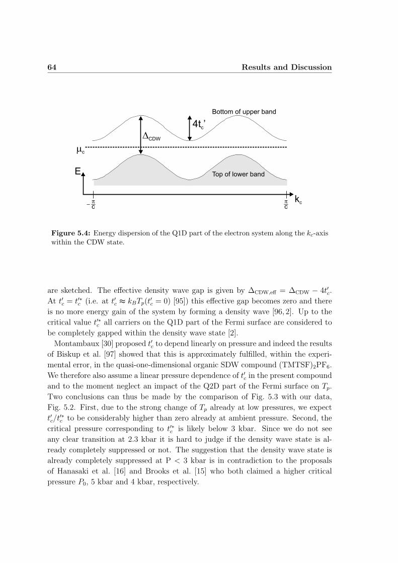
64 Results and Discussion
Top of lower band
Bottom of upper band
mc
4t ’c
DCDW
E
kcpc
pc
Figure 5.4: Energy dispersion of the Q1D part of the electron system along the kc-axiswithin the CDW state.
are sketched. The effective density wave gap is given by ∆CDW,eff = ∆CDW − 4t′c.
At t′c = t′∗c (i.e. at t′c ≈ kBTp(t′c = 0) [95]) this effective gap becomes zero and there
is no more energy gain of the system by forming a density wave [96, 2]. Up to the
critical value t′∗c all carriers on the Q1D part of the Fermi surface are considered to
be completely gapped within the density wave state [2].
Montambaux [30] proposed t′c to depend linearly on pressure and indeed the results
of Biskup et al. [97] showed that this is approximately fulfilled, within the experi-
mental error, in the quasi-one-dimensional organic SDW compound (TMTSF)2PF6.
We therefore also assume a linear pressure dependence of t′c in the present compound
and to the moment neglect an impact of the Q2D part of the Fermi surface on Tp.
Two conclusions can thus be made by the comparison of Fig. 5.3 with our data,
Fig. 5.2. First, due to the strong change of Tp already at low pressures, we expect
t′c/t′∗c to be considerably higher than zero already at ambient pressure. Second, the
critical pressure corresponding to t′∗c is likely below 3 kbar. Since we do not see
any clear transition at 2.3 kbar it is hard to judge if the density wave state is al-
ready completely suppressed or not. The suggestion that the density wave state is
already completely suppressed at P < 3 kbar is in contradiction to the proposals
of Hanasaki et al. [16] and Brooks et al. [15] who both claimed a higher critical
pressure P0, 5 kbar and 4 kbar, respectively.

5.1 The CDW Ground State under Hydrostatic Pressure 65
5.1.2 Magnetoresistance
Determination of B-T Phase Lines via Kohler’s Rule
All the data presented in this chapter were measured in a magnetic field applied
perpendicular to the conducting layers. Fig. 5.5 shows typical temperature sweeps
of the magnetoresistance taken at several constant fields at ambient pressure and at4He-pressure of 1.6 kbar. The CDW state is characterized by its strong magnetore-
sistance most probably emerging due to carriers running along the open sheets of the
reconstructed Fermi surface. While a general suppression of Tp with pressure is seen
in Fig. 5.5, one can imagine that an exact determination of transition points from
these curves is not straightforward. Different criteria for extracting transition points
has led to various kinds of suggested B-T phase diagrams and therefore to different
proposals concerning the nature of the low temperature ground state [76,77,98].
In this work we give arguments for a reasonable estimation of the phase diagram
via Kohler’s rule, a similarity law for the magnetoresistance (see section 2.4):
RB(T )−R0(T )
R0(T )= F (
B
R0(T )). (5.2)
It is not obvious that BEDT-TTF based metals, possessing such anisotropic electron
systems, should obey Kohler’s rule. However, this rule has already been found to
work well in other organic systems with a metallic state at low temperatures [99,100],
showing that it might also be applicable to the title compound. So-called Kohler
plots (i.e. magnetoresistance vs. the scaled zero-field conductivity) of the curves in
Fig. 5.5 are depicted in Fig. 5.6. The temperature in each curve decreases from the
left to the right. It is seen that the high temperature parts of the curves follow one
general function, in accordance with Kohler’s rule. We therefore suggest the rule
to be valid in the NM state of our compound at the given orientation and range of
magnetic field. At lower temperatures all the curves start to diverge dramatically
that is in line with an earlier report on a strong violation of Kohler’s rule in the
CDW state of the title compound [101]. We therefore ascribe the deviation from
Kohler’s rule to the transition from the NM to the CDW state. As a characteristic
transition temperature Tp we choose here the crossing point of linear extrapolations
from the high and low temperature parts as depicted in Fig. 5.6. The transition
lines extracted in this way are shown for three different pressures in Fig. 5.7. Note-
worthy, other methods of determining Tp, e.g. max. curvature or a typical kink in
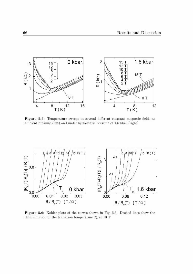
66 Results and Discussion
Figure 5.5: Temperature sweeps at several different constant magnetic fields atambient pressure (left) and under hydrostatic pressure of 1.6 kbar (right).
Figure 5.6: Kohler plots of the curves shown in Fig. 5.5. Dashed lines show thedetermination of the transition temperature Tp at 10 T.
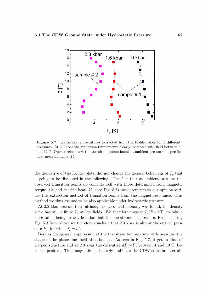
5.1 The CDW Ground State under Hydrostatic Pressure 67
Figure 5.7: Transition temperatures extracted from the Kohler plots for 3 differentpressures. At 2.3 kbar the transition temperature clearly increases with field between 5and 12 T. Open circles mark the transition points found at ambient pressure in specificheat measurements [75]
the derivative of the Kohler plots, did not change the general behaviour of Tp that
is going to be discussed in the following. The fact that at ambient pressure the
observed transition points do coincide well with those determined from magnetic
torque [12] and specific heat [75] (see Fig. 5.7) measurements to our opinion veri-
fies this extraction method of transition points from the magnetoresistance. This
method we thus assume to be also applicable under hydrostatic pressure.
At 2.3 kbar wee see that, although no zero-field anomaly was found, the density
wave has still a finite Tp at low fields. We therefore suggest Tp(B=0 T) to take a
close value, being already less than half the one at ambient pressure. Reconsidering
Fig. 5.3 from above we therefore conclude that 2.3 kbar is almost the critical pres-
sure P0, for which t′c = t′∗c .
Besides the general suppression of the transition temperature with pressure, the
shape of the phase line itself also changes. As seen in Fig. 5.7, it gets a kind of
warped structure and at 2.3 kbar the derivative dTp/dB, between 4 and 10 T, be-
comes positive. Thus magnetic field clearly stabilizes the CDW state in a certain
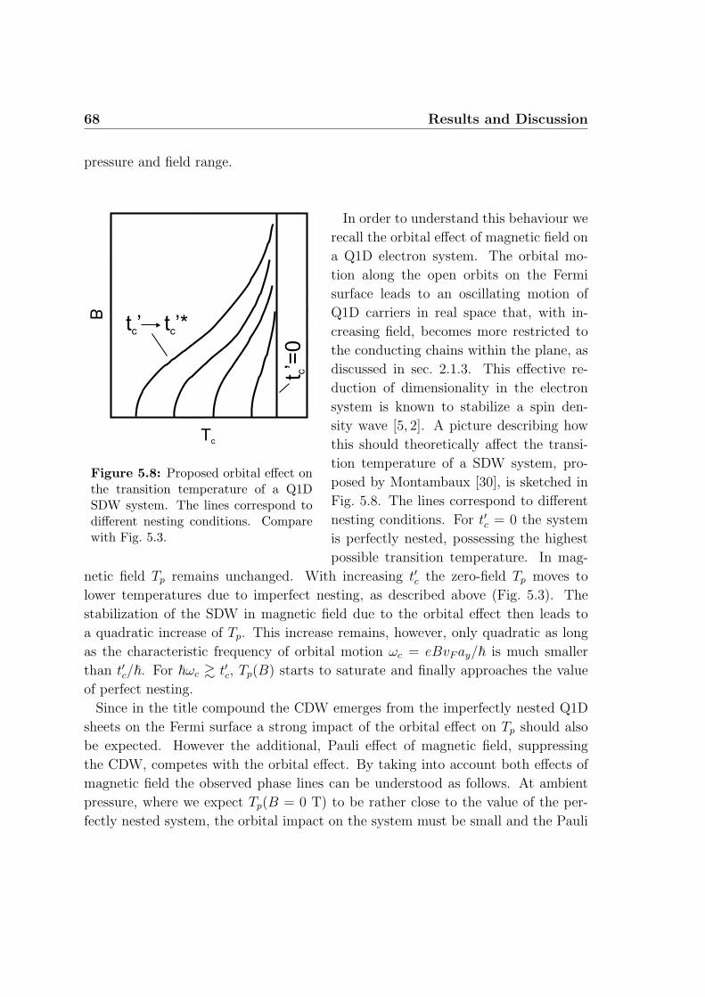
68 Results and Discussion
pressure and field range.
Tc
B
t’=
0c
t ’c
t ’*c
Figure 5.8: Proposed orbital effect onthe transition temperature of a Q1DSDW system. The lines correspond todifferent nesting conditions. Comparewith Fig. 5.3.
In order to understand this behaviour we
recall the orbital effect of magnetic field on
a Q1D electron system. The orbital mo-
tion along the open orbits on the Fermi
surface leads to an oscillating motion of
Q1D carriers in real space that, with in-
creasing field, becomes more restricted to
the conducting chains within the plane, as
discussed in sec. 2.1.3. This effective re-
duction of dimensionality in the electron
system is known to stabilize a spin den-
sity wave [5, 2]. A picture describing how
this should theoretically affect the transi-
tion temperature of a SDW system, pro-
posed by Montambaux [30], is sketched in
Fig. 5.8. The lines correspond to different
nesting conditions. For t′c = 0 the system
is perfectly nested, possessing the highest
possible transition temperature. In mag-
netic field Tp remains unchanged. With increasing t′c the zero-field Tp moves to
lower temperatures due to imperfect nesting, as described above (Fig. 5.3). The
stabilization of the SDW in magnetic field due to the orbital effect then leads to
a quadratic increase of Tp. This increase remains, however, only quadratic as long
as the characteristic frequency of orbital motion ωc = eBvF ay/~ is much smaller
than t′c/~. For ~ωc & t′c, Tp(B) starts to saturate and finally approaches the value
of perfect nesting.
Since in the title compound the CDW emerges from the imperfectly nested Q1D
sheets on the Fermi surface a strong impact of the orbital effect on Tp should also
be expected. However the additional, Pauli effect of magnetic field, suppressing
the CDW, competes with the orbital effect. By taking into account both effects of
magnetic field the observed phase lines can be understood as follows. At ambient
pressure, where we expect Tp(B = 0 T) to be rather close to the value of the per-
fectly nested system, the orbital impact on the system must be small and the Pauli
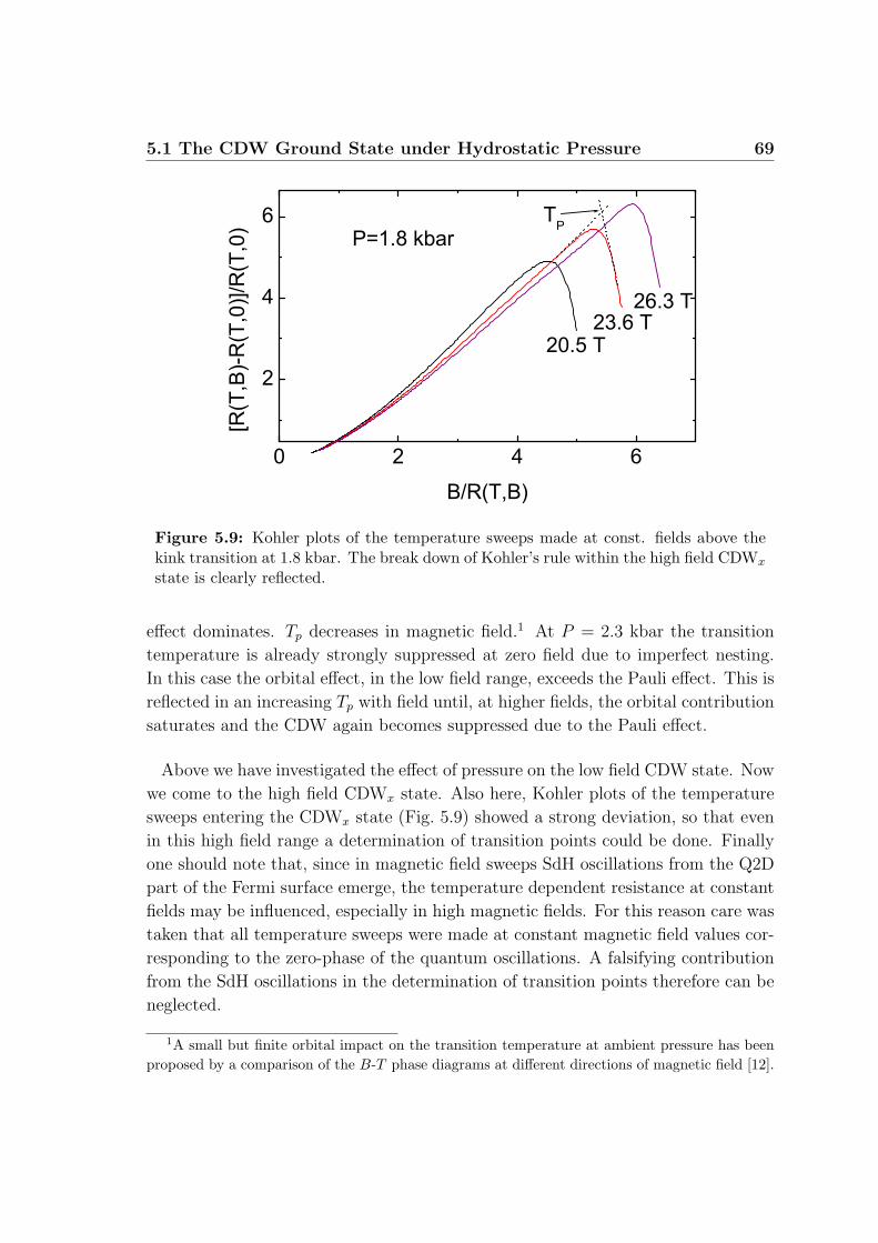
5.1 The CDW Ground State under Hydrostatic Pressure 69
Figure 5.9: Kohler plots of the temperature sweeps made at const. fields above thekink transition at 1.8 kbar. The break down of Kohler’s rule within the high field CDWx
state is clearly reflected.
effect dominates. Tp decreases in magnetic field.1 At P = 2.3 kbar the transition
temperature is already strongly suppressed at zero field due to imperfect nesting.
In this case the orbital effect, in the low field range, exceeds the Pauli effect. This is
reflected in an increasing Tp with field until, at higher fields, the orbital contribution
saturates and the CDW again becomes suppressed due to the Pauli effect.
Above we have investigated the effect of pressure on the low field CDW state. Now
we come to the high field CDWx state. Also here, Kohler plots of the temperature
sweeps entering the CDWx state (Fig. 5.9) showed a strong deviation, so that even
in this high field range a determination of transition points could be done. Finally
one should note that, since in magnetic field sweeps SdH oscillations from the Q2D
part of the Fermi surface emerge, the temperature dependent resistance at constant
fields may be influenced, especially in high magnetic fields. For this reason care was
taken that all temperature sweeps were made at constant magnetic field values cor-
responding to the zero-phase of the quantum oscillations. A falsifying contribution
from the SdH oscillations in the determination of transition points therefore can be
neglected.
1A small but finite orbital impact on the transition temperature at ambient pressure has beenproposed by a comparison of the B-T phase diagrams at different directions of magnetic field [12].
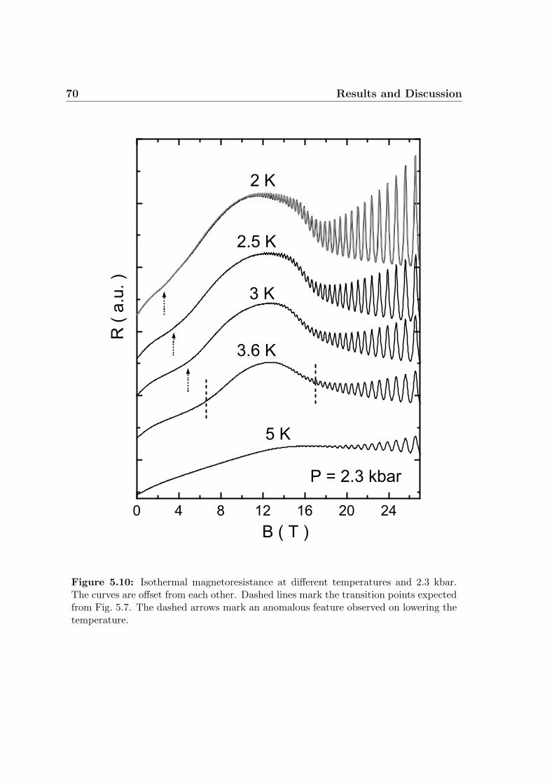
70 Results and Discussion
Figure 5.10: Isothermal magnetoresistance at different temperatures and 2.3 kbar.The curves are offset from each other. Dashed lines mark the transition points expectedfrom Fig. 5.7. The dashed arrows mark an anomalous feature observed on lowering thetemperature.
5.1 The CDW Ground State under Hydrostatic Pressure 71
Before putting all the determined transition points into a combined phase dia-
gram, we first discuss now some experimental results on the field dependence of the
magnetoresistance.
To remind, within isothermal field sweeps at ambient pressure the magnetore-
sistance reaches a maximum that most likely occurs due to magnetic breakdown
between the open sheets and the small lenses on the reconstructed Fermi surface
(see sec. 3.4). At ambient pressure and 1.4 K this maximum of the resistance typi-
cally occurred in the field range of 11-12 T, exceeding the zero-field resistance by a
factor of 20-300. Such a strong sample dependence is thought to be due to different
scattering rates, i.e. different sample qualities. With further enhancing the field
the background magnetoresistance decreases due to a stronger magnetic breakdown
probability until at about 24 T a typical kink characterizes the first order transition
into the high field state. The SdH oscillations start to appear close to the maximum
in the background resistance, in agreement with the breakdown model [85].
We now present changes occurring on applying hydrostatic pressure. A set of
field sweeps taken at 2.3 kbar is shown in Fig. 5.10. For clarity the curves are off-
set from each other. In the low field range (< 10 T) there are clear features seen
in the magnetoresistance. To understand this, a comparison with the transition
points presented in Fig. 5.7 turns out to be helpful. At 5 K the isothermal field
sweep is expected to be completely within the NM state. This is in line with the
observed moderate increase of the magnetoresistance with field showing no sign of
any transition. Such a behaviour is also known to occur in the isostructural com-
pound α−(BEDT-TTF)2NH4Hg(SCN)4, which does not undergo a CDW transition
and is normal metallic at low temperatures. At 3.6 K and 2.3 kbar we expect an
entrance to the low field state at about 6.5 T and a re-establishment of the NM
state at 16.5 T. These fields are marked by dashed lines in the 3.6 K field sweep
in Fig. 5.10. Obviously there is a very good agreement between the temperature
and the field sweeps if one expects the typical increase of the magnetoresistance
within the CDW state. With further lowering the temperature the low field feature
weakens and moves to lower fields, as indicated by the dashed arrows in Fig. 5.10.
Below 3 K the slope of the magnetoresistance near 0 T starts to increase, suggesting
the CDW state already to exist at zero field. The weak feature at low fields still
existing below 3 K we therefore attribute to the vicinity of the phase line and not
to a real transition.
Altogether, the phase line determined from Kohler’s rule is thus clearly reflected
in magnetic field sweeps. The kink transition field , deduced by the crossing point of
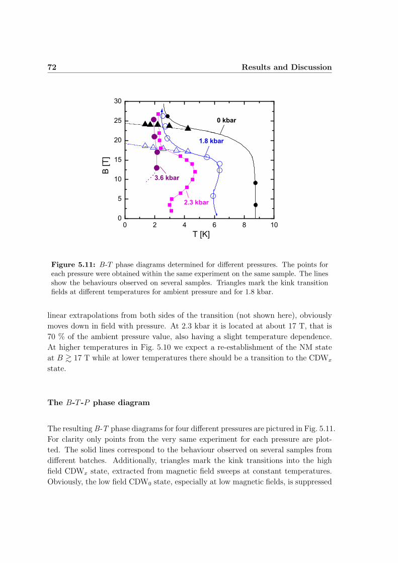
72 Results and Discussion
Figure 5.11: B-T phase diagrams determined for different pressures. The points foreach pressure were obtained within the same experiment on the same sample. The linesshow the behaviours observed on several samples. Triangles mark the kink transitionfields at different temperatures for ambient pressure and for 1.8 kbar.
linear extrapolations from both sides of the transition (not shown here), obviously
moves down in field with pressure. At 2.3 kbar it is located at about 17 T, that is
70 % of the ambient pressure value, also having a slight temperature dependence.
At higher temperatures in Fig. 5.10 we expect a re-establishment of the NM state
at B & 17 T while at lower temperatures there should be a transition to the CDWx
state.
The B-T -P phase diagram
The resulting B-T phase diagrams for four different pressures are pictured in Fig. 5.11.
For clarity only points from the very same experiment for each pressure are plot-
ted. The solid lines correspond to the behaviour observed on several samples from
different batches. Additionally, triangles mark the kink transitions into the high
field CDWx state, extracted from magnetic field sweeps at constant temperatures.
Obviously, the low field CDW0 state, especially at low magnetic fields, is suppressed
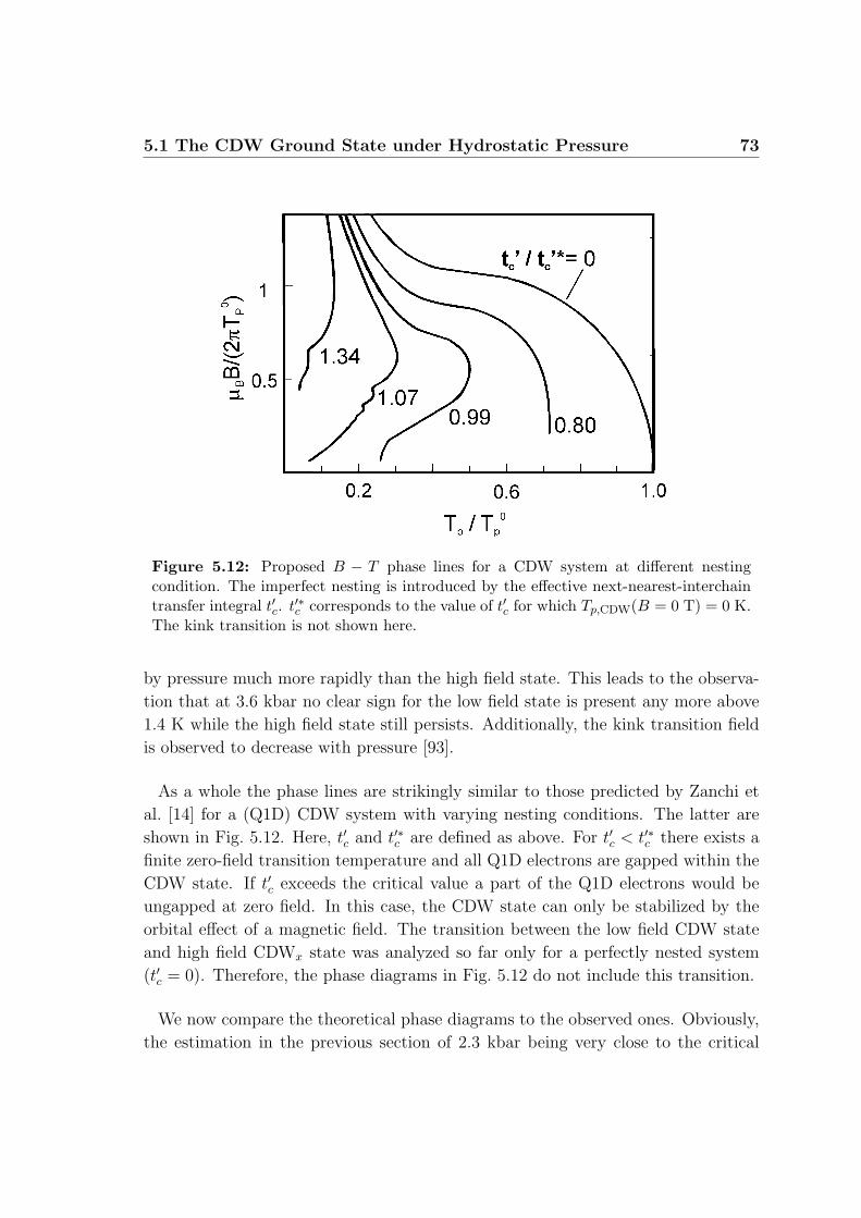
5.1 The CDW Ground State under Hydrostatic Pressure 73
Figure 5.12: Proposed B − T phase lines for a CDW system at different nestingcondition. The imperfect nesting is introduced by the effective next-nearest-interchaintransfer integral t′c. t′∗c corresponds to the value of t′c for which Tp,CDW(B = 0 T) = 0 K.The kink transition is not shown here.
by pressure much more rapidly than the high field state. This leads to the observa-
tion that at 3.6 kbar no clear sign for the low field state is present any more above
1.4 K while the high field state still persists. Additionally, the kink transition field
is observed to decrease with pressure [93].
As a whole the phase lines are strikingly similar to those predicted by Zanchi et
al. [14] for a (Q1D) CDW system with varying nesting conditions. The latter are
shown in Fig. 5.12. Here, t′c and t′∗c are defined as above. For t′c < t′∗c there exists a
finite zero-field transition temperature and all Q1D electrons are gapped within the
CDW state. If t′c exceeds the critical value a part of the Q1D electrons would be
ungapped at zero field. In this case, the CDW state can only be stabilized by the
orbital effect of a magnetic field. The transition between the low field CDW state
and high field CDWx state was analyzed so far only for a perfectly nested system
(t′c = 0). Therefore, the phase diagrams in Fig. 5.12 do not include this transition.
We now compare the theoretical phase diagrams to the observed ones. Obviously,
the estimation in the previous section of 2.3 kbar being very close to the critical
74 Results and Discussion
pressure value corresponding to t′∗c is also reasonable within magnetic field. The
finding that at 3.6 kbar deviations from Kohler’s rule above 1.4 K could only be
found at B > 12 T strongly suggests that here t′c/t′∗c > 1. The proposal made above
that t′c at ambient pressure is considerably higher than zero remains also reasonable,
since we do observe a rather steep phase line at low fields (the designation CDW0
state we will take from now on for the low field CDW state at ambient pressure).
One sees that our experimental observations can be qualitatively well described by
a theoretical CDW model of a Q1D system at different nesting conditions. Thus,
hydrostatic pressure serves as an experimentally accessible parameter that tunes the
nesting conditions of the CDW system. Remarkably, this is the first direct evidence
for an orbital stabilization of a CDW system within magnetic field.2
Yet, we do not pretend to make an explicit quantitative comparison between the
experimental and theoretical phase diagrams here due to several reasons:
• The theoretical phase lines depend to some extend on the values of the coupling
constants [14] which are not known for the present compound;
• The theory does not take into account effects of fluctuations. It is known
that for such a low dimensional CDW system they cannot be neglegted [19].
In many CDW systems the value 2∆/kBT3D well exceeds the weak coupling
BCS result of 2∆/kBT3D = 3.52, suggesting that the transition temperatures
are significantly lower than the mean field transition temperature, TMFCDW [19].
Examples for various CDW compounds are shown in Tab. 5.1.
• In our system there is an additional Q2D-electron band that is theoretically
not taken into account and might also lead to quantitative modifications of
the phase diagram.
Nevertheless, the qualitative physical understanding of our determined B-T phase
diagrams at different pressures gives further strong arguments for the CDW nature of
the present low temperature ground state. This immediately raises some interesting
questions for further experimental investigations, namely:
→ 1. Zanchi et al. [14] predicted successive field-induced CDW transitions to
occur under the conditions tc > t′∗c . Therefore, in order to check the possible
2A possible increase of Tp by ≈ 0.5 K (∆T/Tp ≈ 1%) in a field of 22.6 T in the CDW compoundNbSe3 was mentioned by R.V. Coleman et al. [102]; however, as noted by the authors, this increasedid not exceed their experimental error bar.
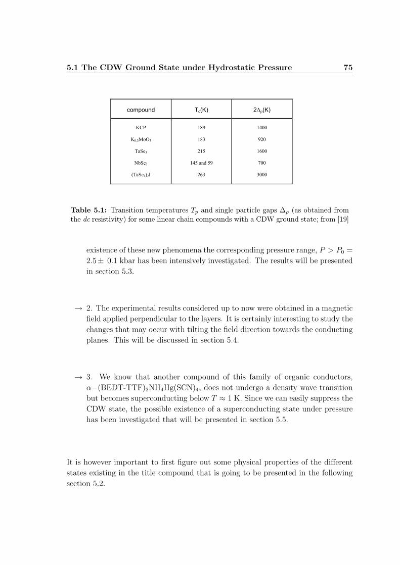
5.1 The CDW Ground State under Hydrostatic Pressure 75
compound Tc(K) 2Dr(K)
KCP
K0.3MoO3
TaSe3
NbSe3
(TaSe4)2I
189
183
215
145 and 59
263
1400
920
1600
700
3000
Table 5.1: Transition temperatures Tp and single particle gaps ∆ρ (as obtained fromthe dc resistivity) for some linear chain compounds with a CDW ground state; from [19]
existence of these new phenomena the corresponding pressure range, P > P0 =
2.5± 0.1 kbar has been intensively investigated. The results will be presented
in section 5.3.
→ 2. The experimental results considered up to now were obtained in a magnetic
field applied perpendicular to the layers. It is certainly interesting to study the
changes that may occur with tilting the field direction towards the conducting
planes. This will be discussed in section 5.4.
→ 3. We know that another compound of this family of organic conductors,
α−(BEDT-TTF)2NH4Hg(SCN)4, does not undergo a density wave transition
but becomes superconducting below T ≈ 1 K. Since we can easily suppress the
CDW state, the possible existence of a superconducting state under pressure
has been investigated that will be presented in section 5.5.
It is however important to first figure out some physical properties of the different
states existing in the title compound that is going to be presented in the following
section 5.2.
76 Results and Discussion
5.1.3 Conclusion
The effect of pressure on the B–T phase diagram of the organic CDW compound
α-(BEDT-TTF)2KHg(SCN)4 was investigated at−→B ⊥ a-c plane.
Hydrostatic pressure is found to suppress the CDW state. At about 2.5 ±0.1 kbar
the CDW is suggested to become completely suppressed at B = 0 T. In order to
extract phase transitions from the magnetoresistance, Kohler’s rule turns out to be
well applicable. The obtained B-T phase diagrams can be consistently interpreted
in terms of an interplay between the Pauli and orbital effects of the magnetic field
on a CDW system. A recent theoretical model of a Q1D CDW system with varying
nesting conditions turns out to describe the observed phase lines remarkably well.
The experimental data thus gives further evidence for a CDW ground state in α-
(BEDT-TTF)2KHg(SCN)4. Altogether, hydrostatic pressure turns out to easily
tune the nesting conditions of the present CDW system. A strong increase of the
transition temperature with magnetic field is found in a certain pressure and field
range. We associate this result with a dramatic enhancement of the orbital effect of
magnetic field due to a deterioration of the nesting conditions by pressure. This is
the first direct evidence for an impact of the orbital carrier motion on the transition
temperature of a CDW system [103].
5.2 Properties of the CDW state 77
5.2 Properties of the CDW state
5.2.1 dHvA and SdH Effects
One of the most direct indications of the reconstructed Fermi surface within the
CDW0 state besides the anomalous angle dependent (semiclassical) magnetoresis-
tance is the appearance of additional frequencies in the spectrum of quantum (SdH
and dHvA) oscillations. For a review on this topic see e.g. [9, 61].
A typical example of the oscillatory magnetoresistance at ambient pressure and
two different temperatures is shown in Fig. 5.13, where the semiclassical (back-
ground) resistance has been removed by dividing by a polynomial fit. As before,
the field is applied perpendicular to the a-c plane. Obviously, different frequencies
are contributing within the CDW0 state whereas in the high field CDWx state one
frequency is dominating. The corresponding fast Fourier transformation (FFT) of
the curves, replotted in inverse field scale, are given in Fig. 5.14. In the CDW0
state three different frequencies and their higher harmonics contribute to the oscil-
lations with different amplitudes. At low temperatures the frequency labeled α, at
≈ 670 T, together with an anomalously high second harmonic content become dom-
inant. Within the CDWx state only α and its moderately strong second harmonic
remain. The α frequency of the oscillation is established not to change on crossing
the high field phase boundary and to also be present within the normal metallic
state. It therefore belongs to the cylindrical or Q2D part of the Fermi surface.
The fact, that the cylindrical Fermi surface gives rise to only one single frequency,
reveals the very high anisotropy of the electron system. This means that the warping
of the cylinder, ∼ 2tb/~vF , must be very small. Otherwise we would see two slightly
different frequencies corresponding to the minimum and maximum cross-sections
and with it a typical beating behavior of the quantum oscillations. Examples for
such a behavior, observed in other organic metals, can be found e.g. in the review
of Wosnitza [9].
Within the CDW0 state additional peaks are observed at frequencies of about
175 T and 850 T, hereafter labeled λ and ν, respectively. These frequencies defi-
nitely cannot be explained by the Fermi surface in the normal metallic state and
must originate from new closed orbits appearing under reconstruction due to the
density wave. While a general suppression of ν on going to temperatures below 1 K
was always found, the relative amplitudes of these frequencies with respect to α
turned out to be strongly sample dependent.
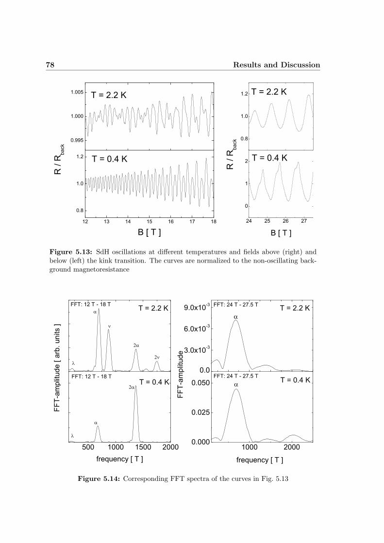
78 Results and Discussion
Figure 5.13: SdH oscillations at different temperatures and fields above (right) andbelow (left) the kink transition. The curves are normalized to the non-oscillating back-ground magnetoresistance
Figure 5.14: Corresponding FFT spectra of the curves in Fig. 5.13
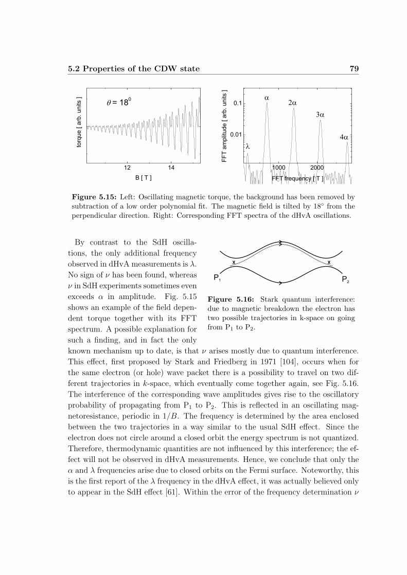
5.2 Properties of the CDW state 79
Figure 5.15: Left: Oscillating magnetic torque, the background has been removed bysubtraction of a low order polynomial fit. The magnetic field is tilted by 18 from theperpendicular direction. Right: Corresponding FFT spectra of the dHvA oscillations.
P2
P1
Figure 5.16: Stark quantum interference:due to magnetic breakdown the electron hastwo possible trajectories in k-space on goingfrom P1 to P2.
By contrast to the SdH oscilla-
tions, the only additional frequency
observed in dHvA measurements is λ.
No sign of ν has been found, whereas
ν in SdH experiments sometimes even
exceeds α in amplitude. Fig. 5.15
shows an example of the field depen-
dent torque together with its FFT
spectrum. A possible explanation for
such a finding, and in fact the only
known mechanism up to date, is that ν arises mostly due to quantum interference.
This effect, first proposed by Stark and Friedberg in 1971 [104], occurs when for
the same electron (or hole) wave packet there is a possibility to travel on two dif-
ferent trajectories in k-space, which eventually come together again, see Fig. 5.16.
The interference of the corresponding wave amplitudes gives rise to the oscillatory
probability of propagating from P1 to P2. This is reflected in an oscillating mag-
netoresistance, periodic in 1/B. The frequency is determined by the area enclosed
between the two trajectories in a way similar to the usual SdH effect. Since the
electron does not circle around a closed orbit the energy spectrum is not quantized.
Therefore, thermodynamic quantities are not influenced by this interference; the ef-
fect will not be observed in dHvA measurements. Hence, we conclude that only the
α and λ frequencies arise due to closed orbits on the Fermi surface. Noteworthy, this
is the first report of the λ frequency in the dHvA effect, it was actually believed only
to appear in the SdH effect [61]. Within the error of the frequency determination ν
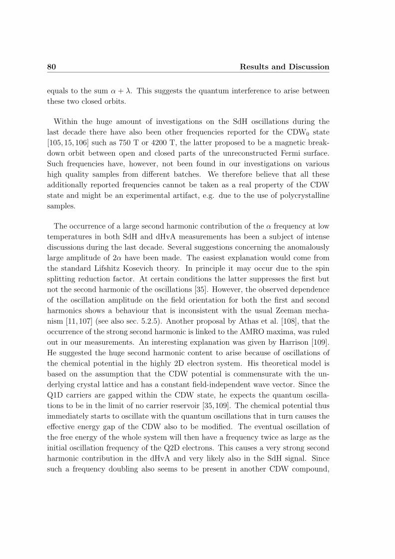
80 Results and Discussion
equals to the sum α + λ. This suggests the quantum interference to arise between
these two closed orbits.
Within the huge amount of investigations on the SdH oscillations during the
last decade there have also been other frequencies reported for the CDW0 state
[105, 15, 106] such as 750 T or 4200 T, the latter proposed to be a magnetic break-
down orbit between open and closed parts of the unreconstructed Fermi surface.
Such frequencies have, however, not been found in our investigations on various
high quality samples from different batches. We therefore believe that all these
additionally reported frequencies cannot be taken as a real property of the CDW
state and might be an experimental artifact, e.g. due to the use of polycrystalline
samples.
The occurrence of a large second harmonic contribution of the α frequency at low
temperatures in both SdH and dHvA measurements has been a subject of intense
discussions during the last decade. Several suggestions concerning the anomalously
large amplitude of 2α have been made. The easiest explanation would come from
the standard Lifshitz Kosevich theory. In principle it may occur due to the spin
splitting reduction factor. At certain conditions the latter suppresses the first but
not the second harmonic of the oscillations [35]. However, the observed dependence
of the oscillation amplitude on the field orientation for both the first and second
harmonics shows a behaviour that is inconsistent with the usual Zeeman mecha-
nism [11,107] (see also sec. 5.2.5). Another proposal by Athas et al. [108], that the
occurrence of the strong second harmonic is linked to the AMRO maxima, was ruled
out in our measurements. An interesting explanation was given by Harrison [109].
He suggested the huge second harmonic content to arise because of oscillations of
the chemical potential in the highly 2D electron system. His theoretical model is
based on the assumption that the CDW potential is commensurate with the un-
derlying crystal lattice and has a constant field-independent wave vector. Since the
Q1D carriers are gapped within the CDW state, he expects the quantum oscilla-
tions to be in the limit of no carrier reservoir [35,109]. The chemical potential thus
immediately starts to oscillate with the quantum oscillations that in turn causes the
effective energy gap of the CDW also to be modified. The eventual oscillation of
the free energy of the whole system will then have a frequency twice as large as the
initial oscillation frequency of the Q2D electrons. This causes a very strong second
harmonic contribution in the dHvA and very likely also in the SdH signal. Since
such a frequency doubling also seems to be present in another CDW compound,
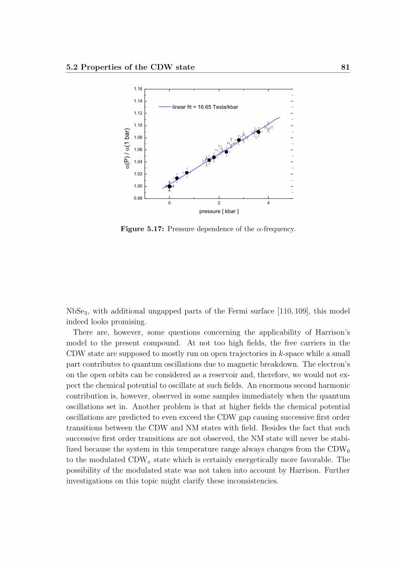
5.2 Properties of the CDW state 81
Figure 5.17: Pressure dependence of the α-frequency.
NbSe3, with additional ungapped parts of the Fermi surface [110, 109], this model
indeed looks promising.
There are, however, some questions concerning the applicability of Harrison’s
model to the present compound. At not too high fields, the free carriers in the
CDW state are supposed to mostly run on open trajectories in k-space while a small
part contributes to quantum oscillations due to magnetic breakdown. The electron’s
on the open orbits can be considered as a reservoir and, therefore, we would not ex-
pect the chemical potential to oscillate at such fields. An enormous second harmonic
contribution is, however, observed in some samples immediately when the quantum
oscillations set in. Another problem is that at higher fields the chemical potential
oscillations are predicted to even exceed the CDW gap causing successive first order
transitions between the CDW and NM states with field. Besides the fact that such
successive first order transitions are not observed, the NM state will never be stabi-
lized because the system in this temperature range always changes from the CDW0
to the modulated CDWx state which is certainly energetically more favorable. The
possibility of the modulated state was not taken into account by Harrison. Further
investigations on this topic might clarify these inconsistencies.
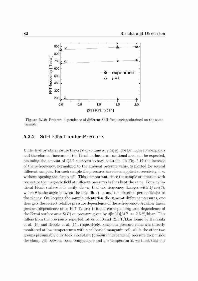
82 Results and Discussion
Figure 5.18: Pressure dependence of different SdH frequencies, obtained on the samesample.
5.2.2 SdH Effect under Pressure
Under hydrostatic pressure the crystal volume is reduced, the Brillouin zone expands
and therefore an increase of the Fermi surface cross-sectional area can be expected,
assuming the amount of Q2D electrons to stay constant. In Fig. 5.17 the increase
of the α-frequency, normalized to the ambient pressure value, is plotted for several
different samples. For each sample the pressures have been applied successively, i. e.
without opening the clamp cell. This is important, since the sample orientation with
respect to the magnetic field at different pressures is thus kept the same. For a cylin-
drical Fermi surface it is easily shown, that the frequency changes with 1/ cos(θ),
where θ is the angle between the field direction and the direction perpendicular to
the planes. On keeping the sample orientation the same at different pressures, one
thus gets the correct relative pressure dependence of the α-frequency. A rather linear
pressure dependence of ≈ 16.7 T/kbar is found corresponding to a dependence of
the Fermi surface area S(P ) on pressure given by d[ln(S)]/dP ≈ 2.5 %/kbar. This
differs from the previously reported values of 10 and 12.1 T/kbar found by Hanasaki
et al. [16] and Brooks et al. [15], respectively. Since our pressure value was directly
monitored at low temperatures with a calibrated manganin coil, while the other two
groups presumably only took a constant (pressure independent) pressure drop inside
the clamp cell between room temperature and low temperatures, we think that our
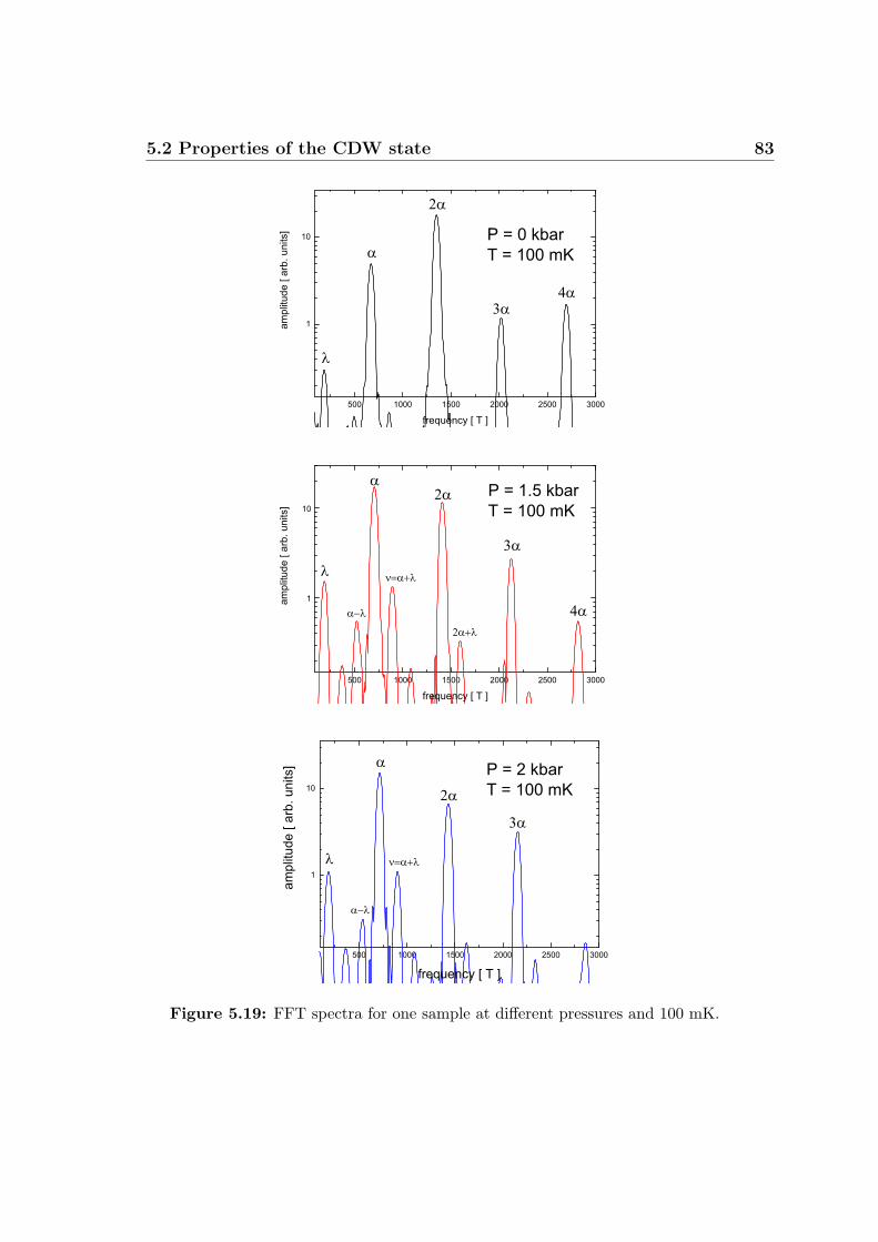
5.2 Properties of the CDW state 83
Figure 5.19: FFT spectra for one sample at different pressures and 100 mK.
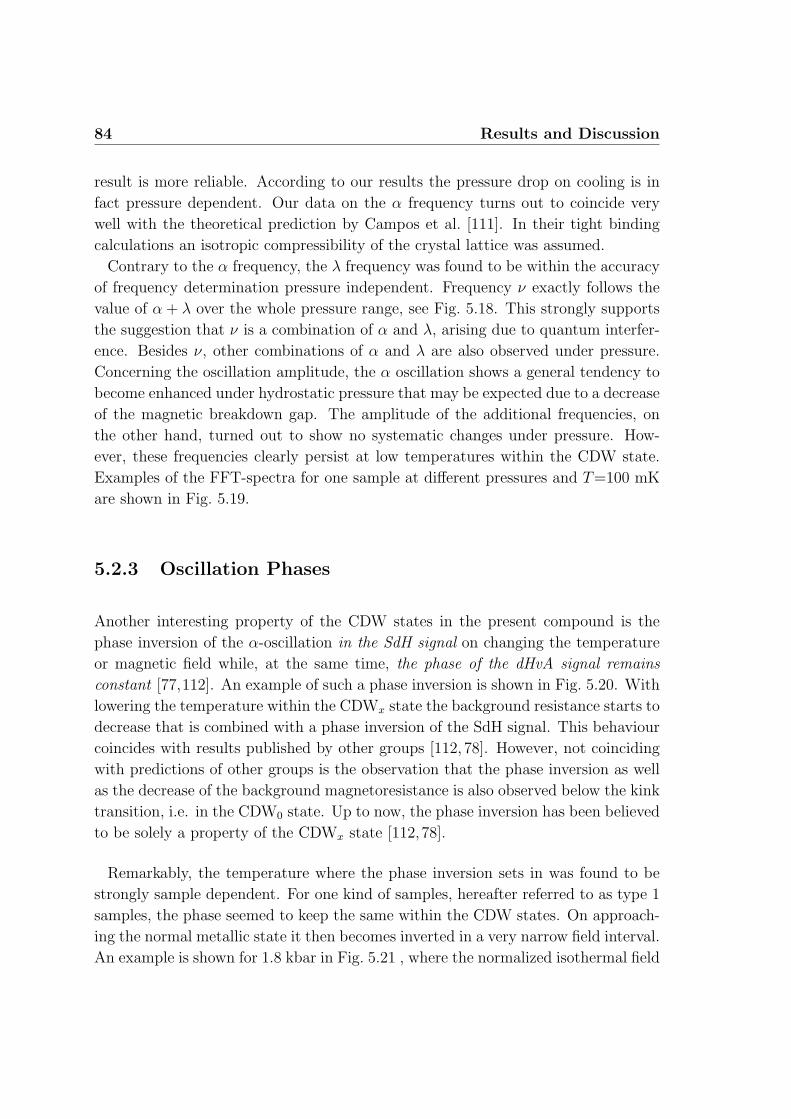
84 Results and Discussion
result is more reliable. According to our results the pressure drop on cooling is in
fact pressure dependent. Our data on the α frequency turns out to coincide very
well with the theoretical prediction by Campos et al. [111]. In their tight binding
calculations an isotropic compressibility of the crystal lattice was assumed.
Contrary to the α frequency, the λ frequency was found to be within the accuracy
of frequency determination pressure independent. Frequency ν exactly follows the
value of α + λ over the whole pressure range, see Fig. 5.18. This strongly supports
the suggestion that ν is a combination of α and λ, arising due to quantum interfer-
ence. Besides ν, other combinations of α and λ are also observed under pressure.
Concerning the oscillation amplitude, the α oscillation shows a general tendency to
become enhanced under hydrostatic pressure that may be expected due to a decrease
of the magnetic breakdown gap. The amplitude of the additional frequencies, on
the other hand, turned out to show no systematic changes under pressure. How-
ever, these frequencies clearly persist at low temperatures within the CDW state.
Examples of the FFT-spectra for one sample at different pressures and T=100 mK
are shown in Fig. 5.19.
5.2.3 Oscillation Phases
Another interesting property of the CDW states in the present compound is the
phase inversion of the α-oscillation in the SdH signal on changing the temperature
or magnetic field while, at the same time, the phase of the dHvA signal remains
constant [77,112]. An example of such a phase inversion is shown in Fig. 5.20. With
lowering the temperature within the CDWx state the background resistance starts to
decrease that is combined with a phase inversion of the SdH signal. This behaviour
coincides with results published by other groups [112, 78]. However, not coinciding
with predictions of other groups is the observation that the phase inversion as well
as the decrease of the background magnetoresistance is also observed below the kink
transition, i.e. in the CDW0 state. Up to now, the phase inversion has been believed
to be solely a property of the CDWx state [112,78].
Remarkably, the temperature where the phase inversion sets in was found to be
strongly sample dependent. For one kind of samples, hereafter referred to as type 1
samples, the phase seemed to keep the same within the CDW states. On approach-
ing the normal metallic state it then becomes inverted in a very narrow field interval.
An example is shown for 1.8 kbar in Fig. 5.21 , where the normalized isothermal field
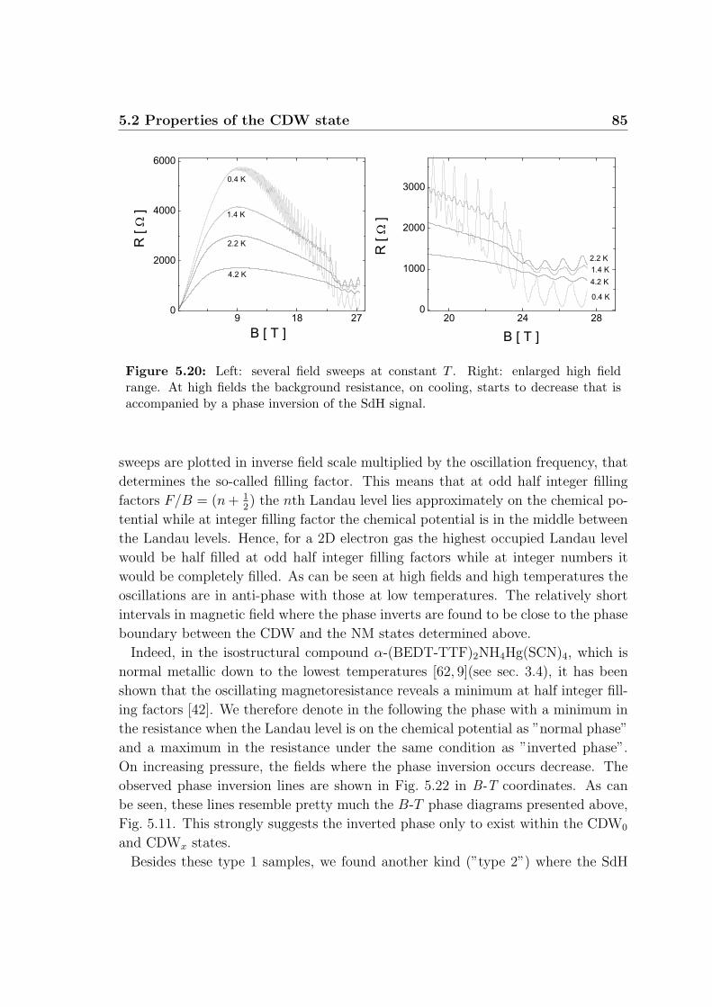
5.2 Properties of the CDW state 85
Figure 5.20: Left: several field sweeps at constant T . Right: enlarged high fieldrange. At high fields the background resistance, on cooling, starts to decrease that isaccompanied by a phase inversion of the SdH signal.
sweeps are plotted in inverse field scale multiplied by the oscillation frequency, that
determines the so-called filling factor. This means that at odd half integer filling
factors F/B = (n + 12) the nth Landau level lies approximately on the chemical po-
tential while at integer filling factor the chemical potential is in the middle between
the Landau levels. Hence, for a 2D electron gas the highest occupied Landau level
would be half filled at odd half integer filling factors while at integer numbers it
would be completely filled. As can be seen at high fields and high temperatures the
oscillations are in anti-phase with those at low temperatures. The relatively short
intervals in magnetic field where the phase inverts are found to be close to the phase
boundary between the CDW and the NM states determined above.
Indeed, in the isostructural compound α-(BEDT-TTF)2NH4Hg(SCN)4, which is
normal metallic down to the lowest temperatures [62, 9](see sec. 3.4), it has been
shown that the oscillating magnetoresistance reveals a minimum at half integer fill-
ing factors [42]. We therefore denote in the following the phase with a minimum in
the resistance when the Landau level is on the chemical potential as ”normal phase”
and a maximum in the resistance under the same condition as ”inverted phase”.
On increasing pressure, the fields where the phase inversion occurs decrease. The
observed phase inversion lines are shown in Fig. 5.22 in B-T coordinates. As can
be seen, these lines resemble pretty much the B-T phase diagrams presented above,
Fig. 5.11. This strongly suggests the inverted phase only to exist within the CDW0
and CDWx states.
Besides these type 1 samples, we found another kind (”type 2”) where the SdH
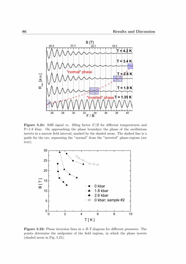
86 Results and Discussion
Figure 5.21: SdH signal vs. filling factor F/B for different temperatures andP=1.8 kbar. On approaching the phase boundary the phase of the oscillationsinverts in a narrow field interval, marked by the shaded areas. The dashed line is aguide for the eye, separating the ”normal” from the ”inverted” phase-regions (seetext).
Figure 5.22: Phase inversion lines in a B-T diagram for different pressures. Thepoints determine the midpoints of the field regions, in which the phase inverts(shaded areas in Fig. 5.21).
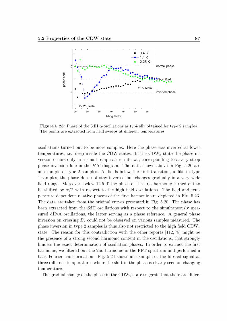
5.2 Properties of the CDW state 87
Figure 5.23: Phase of the SdH α-oscillations as typically obtained for type 2 samples.The points are extracted from field sweeps at different temperatures.
oscillations turned out to be more complex. Here the phase was inverted at lower
temperatures, i.e. deep inside the CDW states. In the CDWx state the phase in-
version occurs only in a small temperature interval, corresponding to a very steep
phase inversion line in the B-T diagram. The data shown above in Fig. 5.20 are
an example of type 2 samples. At fields below the kink transition, unlike in type
1 samples, the phase does not stay inverted but changes gradually in a very wide
field range. Moreover, below 12.5 T the phase of the first harmonic turned out to
be shifted by π/2 with respect to the high field oscillations. The field and tem-
perature dependent relative phases of the first harmonic are depicted in Fig. 5.23.
The data are taken from the original curves presented in Fig. 5.20. The phase has
been extracted from the SdH oscillations with respect to the simultaneously mea-
sured dHvA oscillations, the latter serving as a phase reference. A general phase
inversion on crossing Bk could not be observed on various samples measured. The
phase inversion in type 2 samples is thus also not restricted to the high field CDWx
state. The reason for this contradiction with the other reports [112, 78] might be
the presence of a strong second harmonic content in the oscillations, that strongly
hinders the exact determination of oscillation phases. In order to extract the first
harmonic, we filtered out the 2nd harmonic in the FFT spectrum and performed a
back Fourier transformation. Fig. 5.24 shows an example of the filtered signal at
three different temperatures where the shift in the phase is clearly seen on changing
temperature.
The gradual change of the phase in the CDW0 state suggests that there are differ-
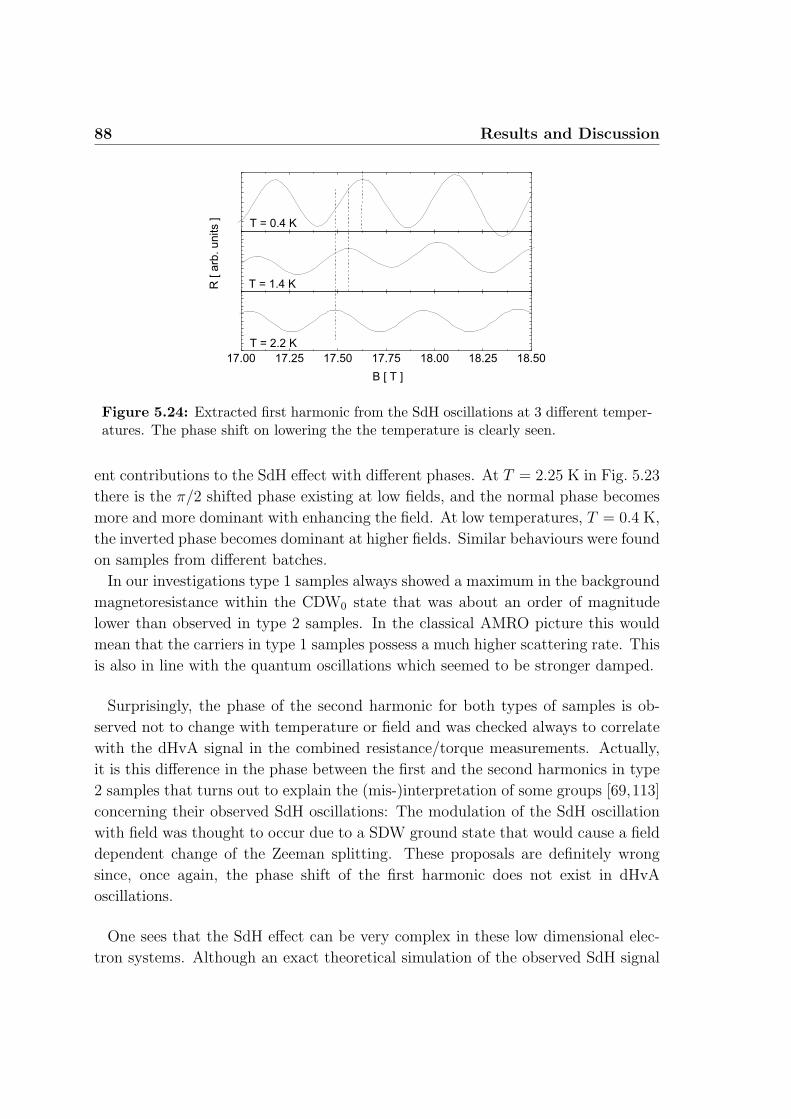
88 Results and Discussion
Figure 5.24: Extracted first harmonic from the SdH oscillations at 3 different temper-atures. The phase shift on lowering the the temperature is clearly seen.
ent contributions to the SdH effect with different phases. At T = 2.25 K in Fig. 5.23
there is the π/2 shifted phase existing at low fields, and the normal phase becomes
more and more dominant with enhancing the field. At low temperatures, T = 0.4 K,
the inverted phase becomes dominant at higher fields. Similar behaviours were found
on samples from different batches.
In our investigations type 1 samples always showed a maximum in the background
magnetoresistance within the CDW0 state that was about an order of magnitude
lower than observed in type 2 samples. In the classical AMRO picture this would
mean that the carriers in type 1 samples possess a much higher scattering rate. This
is also in line with the quantum oscillations which seemed to be stronger damped.
Surprisingly, the phase of the second harmonic for both types of samples is ob-
served not to change with temperature or field and was checked always to correlate
with the dHvA signal in the combined resistance/torque measurements. Actually,
it is this difference in the phase between the first and the second harmonics in type
2 samples that turns out to explain the (mis-)interpretation of some groups [69,113]
concerning their observed SdH oscillations: The modulation of the SdH oscillation
with field was thought to occur due to a SDW ground state that would cause a field
dependent change of the Zeeman splitting. These proposals are definitely wrong
since, once again, the phase shift of the first harmonic does not exist in dHvA
oscillations.
One sees that the SdH effect can be very complex in these low dimensional elec-
tron systems. Although an exact theoretical simulation of the observed SdH signal
5.2 Properties of the CDW state 89
cannot be done at the moment, some qualitative remarks will be given in the fol-
lowing. Since this is a rather special topic, we note here that the discussion below
is not needed for understanding further results presented in this thesis.
Normally, the SdH effect for the longitudinal interlayer magnetoconductivity in or-
ganic salts with such ”highly” Q2D electron systems is considered via the Boltzmann
transport equation:
σzz = e2
∫dε
df(ε)
dεI(ε)τ(ε) (5.3)
where f(ε) is the Fermi distribution function, I(ε) ≡∑| vz(ε) |2 is the square of
the electron velocity summed over all states at the energy ε, vz is the interlayer-
component of the electron velocity and τ(ε) is the momentum relaxation time at
energy ε. At high enough fields, we can assume the distance between subsequent
Landau levels ~ωc to become bigger than the interlayer bandwidth of the Fermi
surface, 4t⊥. If then the chemical potential lies in between the Landau levels, the
velocity at the Fermi level,
vz(εF ) =1
~∂ε
∂kz
∣∣ε'εF
(5.4)
simply becomes zero. By taking into account the broadening of the levels due to a
finite scattering time, the velocity is finite but takes a minimum value. In this case
the term I(ε) in Eq. (5.3) determines the phase of the oscillation and one expects
a minimum in the magnetoresistance at half integer filling factors, i.e. the normal
phase (see Fig. 5.21).
For type 1 samples, we know that in the low field CDW0 state the phase is in-
verted. This might be explained by assuming that the density of states oscillation
rather than the oscillation of the interlayer velocity determines the phase of the
quantum oscillations (after Fermi’s golden rule the scattering rate is, to the first
order, proportional to the number of states into which scattering is possible). This
would mean that in the CDW0 state the SdH oscillations are probably better de-
scribed by conventional (3D) SdH theories, in which the scattering rate determines
the oscillation phase. A crossover at the phase boundary between the CDW and the
NM states would then cause a node in the SdH oscillations, combined with a phase
inversion. Such a crossover might explain the behaviour observed in type 1 samples.
It is, however, not understood at present why within the CDW0 state solely the
scattering rate should determine the oscillation phase.
The smooth phase shift over a wide field range in type 2 samples in the low field
CDW0 state must have a different origin. It might be caused by an interplay of
the two oscillating terms in Eq. (5.3), i.e. the carrier velocity and scattering rate.
90 Results and Discussion
The change from the π/2-shifted to the normal phase with field may arise due to an
increasing contribution of the carrier velocity to the total oscillation of the conduc-
tivity. Another possibility could be the presence of different scattering mechanisms.
As has already been pointed out in the early works by Adams and Holstein [40] and
Lifshitz and Kosevich [114] two terms add up to give the net (3D) SdH oscillation,
one involving inter-Landau band scattering the other intra-Landau band scattering.
For not too high fields, i.e. at large quantum numbers the first term may even give
the major contribution to the quantum oscillation in the transverse conductivity.
Indeed, the possibility of a phase difference between both contributions to the SdH
oscillations has also been predicted [40].
Which mechanism eventually leads to such a strong phase shift in the longitudinal
magnetoresistance with magnetic field as observed in type 2 samples is not clear,
since a detailed theoretical description is still missing. Moreover, it is not clear to
the moment if magnetic breakdown also affects the phase of the SdH oscillation.
A detailed theoretical analysis of the SdH effect of Q2D electron systems at differ-
ent fields and temperatures is needed for a comparison with our experimental data.
We emphasize here, that as long as this complex behaviour in the SdH effect is not
understood, a reliable extraction of such values as m∗, g∗m∗, and TD from the SdH
signal cannot be done and all reports based on the SdH effect must be considered
with great care.
Remarkably, the phase inversion at low temperatures and high fields, illustrated in
Fig. 5.20, always occurs together with a strong decrease of the semiclassical (back-
ground) magnetoresistance. This is observed on all samples investigated. We, there-
fore, believe these two effects to be directly related to each other. In other words:
as soon as the background resistance starts to decrease the phase becomes inverted.
Obviously, an additional, at low temperature even dominating, contribution to the
conductivity emerges. This could probably explain the phase inversion. At odd half
integer filling factors, i.e. when the Landau level is on the chemical potential, there
are more states into which the carriers of this additional conduction channel can
scatter. The total resistance therefore increases. Correspondingly, at integer filling
factors we then observe a minimum of the resistance. The nature of this additional
conductivity contribution to the moment is however not clear. It might originate
from partially ungapped Q1D carriers, which are indeed expected within the CDWx
state, but not at fields below the kink transition. Another possibility for an addi-
tional contribution to the conductivity is a sliding CDW. This collective motion of
the carriers might occur within the CDW state [19]. How this can affect the phase
5.2 Properties of the CDW state 91
of the SdH oscillations is, however, not clear at present.
5.2.4 Magnetic Torque within the Modulated CDWx State
Up to now there is a general agreement about the existence of the CDWx state at
high fields and low temperatures that was first proposed by McKenzie in 1997 [13].
It demarcates itself from the NM one in several distinct properties:
• As was shown by Christ et al. the phase boundary is directly reflected in a
change of slope in the temperature dependent magnetic torque at constant
field [74,12,77].
• In the magnetoresistance a rather strong decrease of the background resistance
combined, at low temperatures, with the phase inversion in the SdH signal is
typically seen in most of the samples [77,112,78].
• Latest AMRO experiments by Kartsovnik et al. showed clear signs of the Q1D
AMROs at high tilt angles even at fields above Bk. This can be expected, since
with tilting the field the magnetic breakdown gap on the closed orbits should
increase and the 2D AMROs should diminish. In the NM state the 2D AMROs
are known to dominate over the whole angular range.
• Additionally, the torque signal below ≈ 2 K was found to be hysteretic in field
within the CDWx state [73,78]. This point we investigated in more detail.
Fig. 5.25 shows the typical behaviour observed in the magnetic torque within the
CDWx state. The background of the magnetic torque shows a considerable hysteresis
on sweeping the field up and down. The hysteresis appears to be of diamagnetic
origin. Note that this hysteresis has nothing to do with the first order kink transition
at 24 T, since it exists up to the highest fields measured. Harrison et al. even showed
that this hysteresis persists at low temperatures in magnetic fields up to the highest
field of their experiments, 32 T [78]. We also emphasize that by no means this
hysteresis can be simply ascribed to the oscillatory part of the torque signal. The
hysteresis definitely appears in the background of the torque. Only with lowering the
temperature the magnitude of the hysteresis was shown to become slightly dependent
on the phase of the oscillation at B > 28 T [78]. This is likely related to the observed
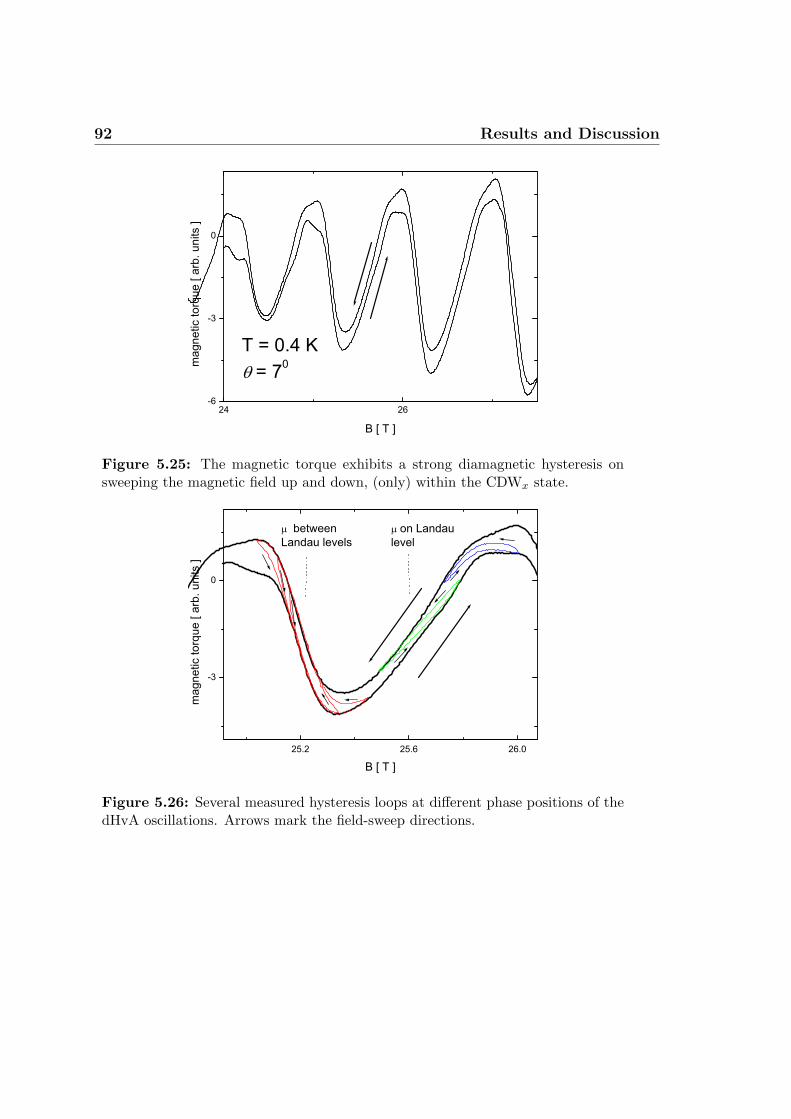
92 Results and Discussion
Figure 5.25: The magnetic torque exhibits a strong diamagnetic hysteresis onsweeping the magnetic field up and down, (only) within the CDWx state.
Figure 5.26: Several measured hysteresis loops at different phase positions of thedHvA oscillations. Arrows mark the field-sweep directions.
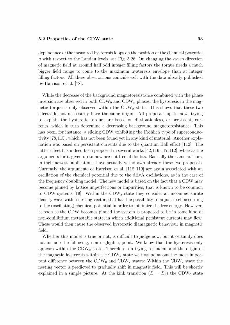
5.2 Properties of the CDW state 93
dependence of the measured hysteresis loops on the position of the chemical potential
µ with respect to the Landau levels, see Fig. 5.26: On changing the sweep direction
of magnetic field at around half odd integer filling factors the torque needs a much
bigger field range to come to the maximum hysteresis envelope than at integer
filling factors. All these observations coincide well with the data already published
by Harrison et al. [78].
While the decrease of the background magnetoresistance combined with the phase
inversion are observed in both CDW0 and CDWx phases, the hysteresis in the mag-
netic torque is only observed within the CDWx state. This shows that these two
effects do not necessarily have the same origin. All proposals up to now, trying
to explain the hysteretic torque, are based on dissipationless, or persistent, cur-
rents, which in turn determine a decreasing background magnetoresistance. This
has been, for instance, a sliding CDW exhibiting the Frohlich type of superconduc-
tivity [78,115], which has not been found yet in any kind of material. Another expla-
nation was based on persistent currents due to the quantum Hall effect [112]. The
latter effect has indeed been proposed in several works [42,116,117,112], whereas the
arguments for it given up to now are not free of doubts. Basically the same authors,
in their newest publications, have actually withdrawn already these two proposals.
Currently, the arguments of Harrison et al. [118, 119] are again associated with an
oscillation of the chemical potential due to the dHvA oscillations, as in the case of
the frequency doubling model. The new model is based on the fact that a CDW may
become pinned by lattice imperfections or impurities, that is known to be common
to CDW systems [19]. Within the CDWx state they consider an incommensurate
density wave with a nesting vector, that has the possibility to adjust itself according
to the (oscillating) chemical potential in order to minimize the free energy. However,
as soon as the CDW becomes pinned the system is proposed to be in some kind of
non-equilibrium metastable state, in which additional persistent currents may flow.
These would then cause the observed hysteretic diamagnetic behaviour in magnetic
field.
Whether this model is true or not, is difficult to judge now, but it certainly does
not include the following, non negligible, point. We know that the hysteresis only
appears within the CDWx state. Therefore, on trying to understand the origin of
the magnetic hysteresis within the CDWx state we first point out the most impor-
tant difference between the CDW0 and CDWx states: Within the CDWx state the
nesting vector is predicted to gradually shift in magnetic field. This will be shortly
explained in a simple picture. At the kink transition (B = Bk) the CDW0 state
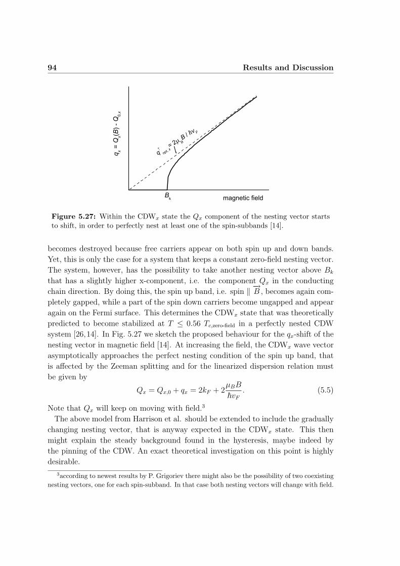
94 Results and Discussion
Figure 5.27: Within the CDWx state the Qx component of the nesting vector startsto shift, in order to perfectly nest at least one of the spin-subbands [14].
becomes destroyed because free carriers appear on both spin up and down bands.
Yet, this is only the case for a system that keeps a constant zero-field nesting vector.
The system, however, has the possibility to take another nesting vector above Bk
that has a slightly higher x-component, i.e. the component Qx in the conducting
chain direction. By doing this, the spin up band, i.e. spin ‖−→B , becomes again com-
pletely gapped, while a part of the spin down carriers become ungapped and appear
again on the Fermi surface. This determines the CDWx state that was theoretically
predicted to become stabilized at T ≤ 0.56 Tc,zero-field in a perfectly nested CDW
system [26,14]. In Fig. 5.27 we sketch the proposed behaviour for the qx-shift of the
nesting vector in magnetic field [14]. At increasing the field, the CDWx wave vector
asymptotically approaches the perfect nesting condition of the spin up band, that
is affected by the Zeeman splitting and for the linearized dispersion relation must
be given by
Qx = Qx,0 + qx = 2kF + 2µBB
~vF
. (5.5)
Note that Qx will keep on moving with field.3
The above model from Harrison et al. should be extended to include the gradually
changing nesting vector, that is anyway expected in the CDWx state. This then
might explain the steady background found in the hysteresis, maybe indeed by
the pinning of the CDW. An exact theoretical investigation on this point is highly
desirable.
3according to newest results by P. Grigoriev there might also be the possibility of two coexistingnesting vectors, one for each spin-subband. In that case both nesting vectors will change with field.
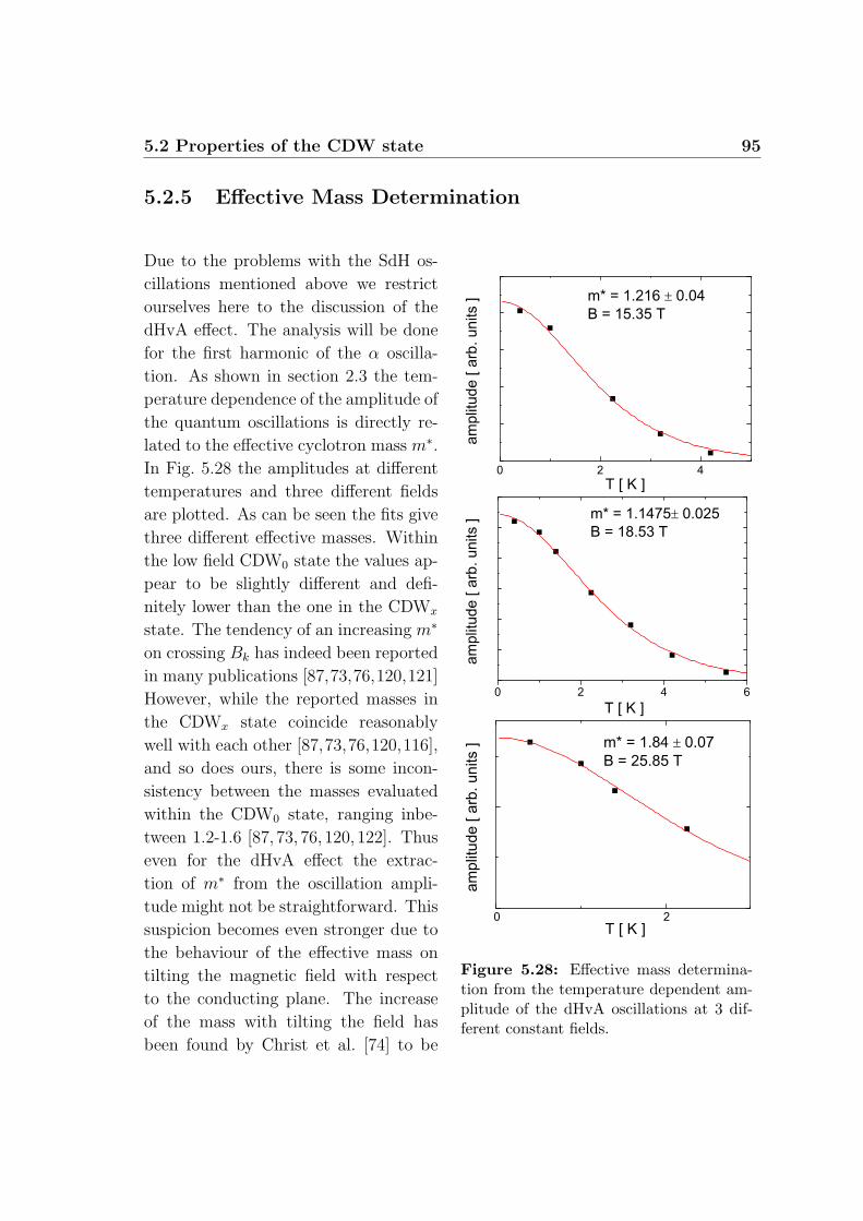
5.2 Properties of the CDW state 95
5.2.5 Effective Mass Determination
Figure 5.28: Effective mass determina-tion from the temperature dependent am-plitude of the dHvA oscillations at 3 dif-ferent constant fields.
Due to the problems with the SdH os-
cillations mentioned above we restrict
ourselves here to the discussion of the
dHvA effect. The analysis will be done
for the first harmonic of the α oscilla-
tion. As shown in section 2.3 the tem-
perature dependence of the amplitude of
the quantum oscillations is directly re-
lated to the effective cyclotron mass m∗.
In Fig. 5.28 the amplitudes at different
temperatures and three different fields
are plotted. As can be seen the fits give
three different effective masses. Within
the low field CDW0 state the values ap-
pear to be slightly different and defi-
nitely lower than the one in the CDWx
state. The tendency of an increasing m∗
on crossing Bk has indeed been reported
in many publications [87,73,76,120,121]
However, while the reported masses in
the CDWx state coincide reasonably
well with each other [87,73,76,120,116],
and so does ours, there is some incon-
sistency between the masses evaluated
within the CDW0 state, ranging inbe-
tween 1.2-1.6 [87, 73, 76, 120, 122]. Thus
even for the dHvA effect the extrac-
tion of m∗ from the oscillation ampli-
tude might not be straightforward. This
suspicion becomes even stronger due to
the behaviour of the effective mass on
tilting the magnetic field with respect
to the conducting plane. The increase
of the mass with tilting the field has
been found by Christ et al. [74] to be
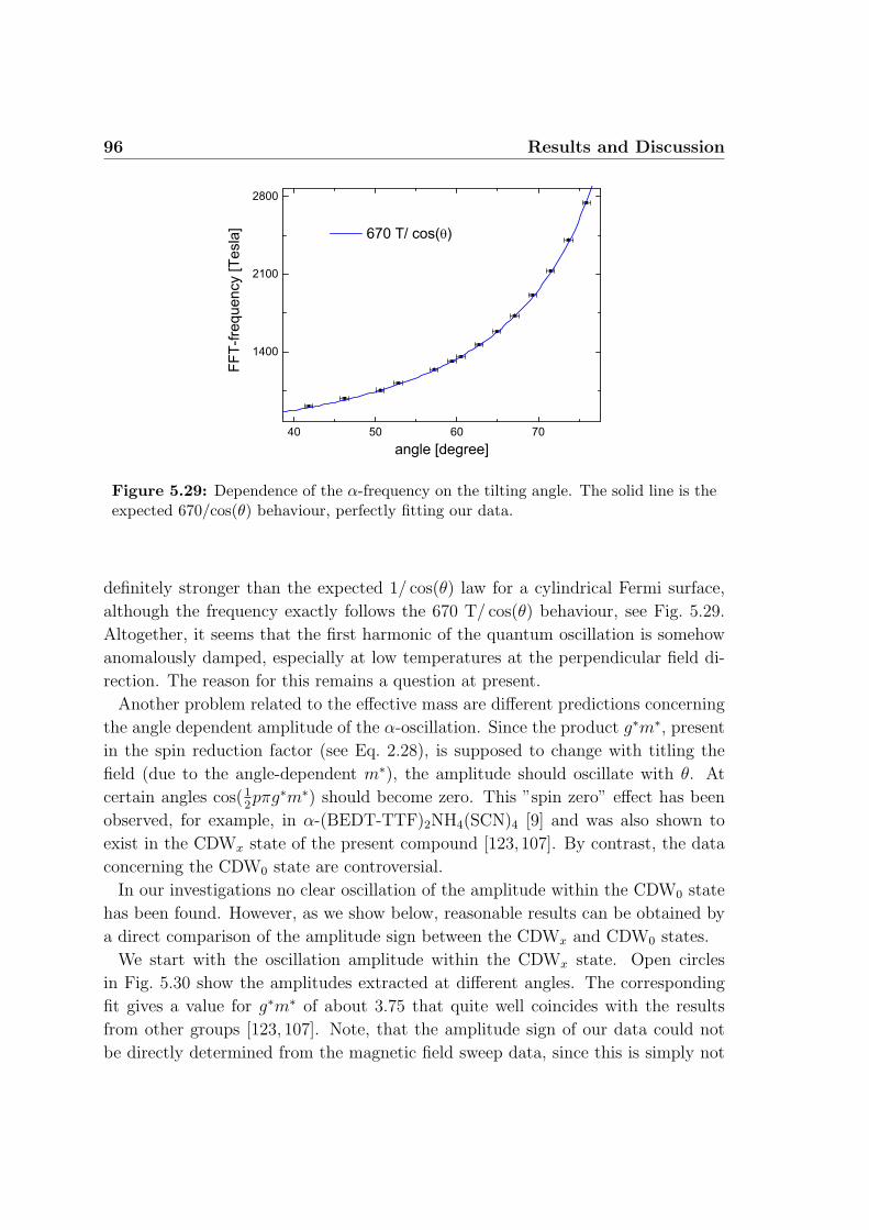
96 Results and Discussion
Figure 5.29: Dependence of the α-frequency on the tilting angle. The solid line is theexpected 670/cos(θ) behaviour, perfectly fitting our data.
definitely stronger than the expected 1/ cos(θ) law for a cylindrical Fermi surface,
although the frequency exactly follows the 670 T/ cos(θ) behaviour, see Fig. 5.29.
Altogether, it seems that the first harmonic of the quantum oscillation is somehow
anomalously damped, especially at low temperatures at the perpendicular field di-
rection. The reason for this remains a question at present.
Another problem related to the effective mass are different predictions concerning
the angle dependent amplitude of the α-oscillation. Since the product g∗m∗, present
in the spin reduction factor (see Eq. 2.28), is supposed to change with titling the
field (due to the angle-dependent m∗), the amplitude should oscillate with θ. At
certain angles cos(12pπg∗m∗) should become zero. This ”spin zero” effect has been
observed, for example, in α-(BEDT-TTF)2NH4(SCN)4 [9] and was also shown to
exist in the CDWx state of the present compound [123, 107]. By contrast, the data
concerning the CDW0 state are controversial.
In our investigations no clear oscillation of the amplitude within the CDW0 state
has been found. However, as we show below, reasonable results can be obtained by
a direct comparison of the amplitude sign between the CDWx and CDW0 states.
We start with the oscillation amplitude within the CDWx state. Open circles
in Fig. 5.30 show the amplitudes extracted at different angles. The corresponding
fit gives a value for g∗m∗ of about 3.75 that quite well coincides with the results
from other groups [123, 107]. Note, that the amplitude sign of our data could not
be directly determined from the magnetic field sweep data, since this is simply not
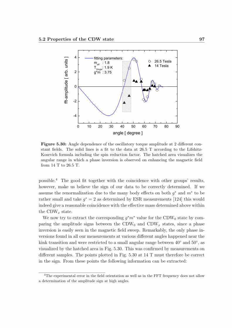
5.2 Properties of the CDW state 97
Figure 5.30: Angle dependence of the oscillatory torque amplitude at 2 different con-stant fields. The solid lines is a fit to the data at 26.5 T according to the Lifshitz-Kosevich formula including the spin reduction factor. The hatched area visualizes theangular range in which a phase inversion is observed on enhancing the magnetic fieldfrom 14 T to 26.5 T.
possible.4 The good fit together with the coincidence with other groups’ results,
however, make us believe the sign of our data to be correctly determined. If we
assume the renormalization due to the many body effects on both g∗ and m∗ to be
rather small and take g∗ = 2 as determined by ESR measurements [124] this would
indeed give a reasonable coincidence with the effective mass determined above within
the CDWx state.
We now try to extract the corresponding g∗m∗ value for the CDW0 state by com-
paring the amplitude signs between the CDW0 and CDWx states, since a phase
inversion is easily seen in the magnetic field sweep. Remarkably, the only phase in-
versions found in all our measurements at various different angles happened near the
kink transition and were restricted to a small angular range between 40 and 50, as
visualized by the hatched area in Fig. 5.30. This was confirmed by measurements on
different samples. The points plotted in Fig. 5.30 at 14 T must therefore be correct
in the sign. From these points the following information can be extracted:
4The experimental error in the field orientation as well as in the FFT frequency does not allowa determination of the amplitude sign at high angles.
98 Results and Discussion
1. The extracted points at 14 T definitely cannot be fitted by the standard
Lifshitz-Kosevich model over the whole angular range. This might explain
the inconsistency in the g∗m∗ values observed by different groups [123,107].
2. At lower angles, assuming g∗ ≈ 2 to be fulfilled, m∗ in the CDW0 state is
definitely lower than in the high field CDWx state. This coincides with the
observed enhancement of m∗ on crossing Bk.
3. In the high angle range, θ > 60, both masses above and below Bk must be
very close to each other. Otherwise we would have further changes in the sign
of the amplitude at sweeping the field, which, however, is not observed.
Summarizing, the effective mass at 14 T indeed seems to change, on tilting the
magnetic field, stronger than the expected 1/ cos(θ) behaviour. As we will show
later in this thesis (section 5.4), it is very likely that at a certain tilt angle there is
a phase transition that would actually explain the third point from above.
5.3 The Re-Entrant CDW State 99
5.3 The Re-Entrant CDW State
5.3.1 Stabilization of the CDW in Magnetic Field
The B-T phase diagrams presented in section 5.1, have shown that hydrostatic pres-
sure is a parameter that tunes the nesting conditions of the density wave remarkably
well. The critical pressure P0, at which the density wave transition temperature at
zero-field becomes 0 K, was estimated to be about 2.5 ± 0.1 kbar. Above P0 we
expect the CDW state only to become stabilized via the orbital effect of magnetic
field. This field-induced state corresponding to t′c > t′∗c we call re-entrant CDW
state. In this section we point out the changes seen in the magnetoresistance which
occur on crossing P0. In particular we give further experimental evidence that the
CDW is really suppressed at low fields and reappears at higher fields at P > P0. As
before the field is directed in the interlayer direction.
Fig. 5.31 shows magnetic field sweeps up to 15 T at the lowest possible temperature
of our experimental setup, for different pressures covering the whole pressure range
investigated within this work. The data presented in Fig. 5.31 are obtained on
the same sample and have been qualitatively reproduced on another one measured
at the same time. At P < 2.5 kbar we expect the density wave to exist at zero-
field. The decrease of the maximum in the semiclassical resistance with pressure
we attribute to a reduced breakdown gap on the reconstructed Fermi surface due
to the worsening of the nesting conditions. The carriers have a higher probability
to tunnel between the open and closed parts of the Fermi surface that causes the
magnetoresistance, dominated by the motion of the carriers along the open sheets,
to become reduced [85]. This then also explains the fact that the maximum of the
magnetoresistance at 1.5 kbar and 2 kbar is found at ≈ 7.5 T that is clearly below
the ambient pressure value of ≈ 11 T. However, we still consider the carriers to
mainly run on the Q1D sheets of the reconstructed Fermi surface thus providing a
rather strong magnetoresistance.
Remarkably, distinct changes occur in the field sweeps on crossing P0. What is
immediately recognized are rather slow oscillations of the background resistance
starting from P = 2.5 kbar. With pressure these oscillations move gradually to
higher fields as visualized by dashed lines in Fig. 5.31.
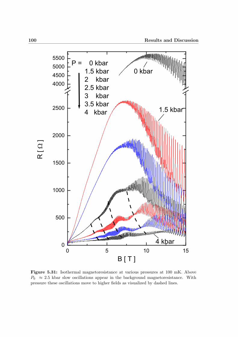
100 Results and Discussion
Figure 5.31: Isothermal magnetoresistance at various pressures at 100 mK. AboveP0 ≈ 2.5 kbar slow oscillations appear in the background magnetoresistance. Withpressure these oscillations move to higher fields as visualized by dashed lines.
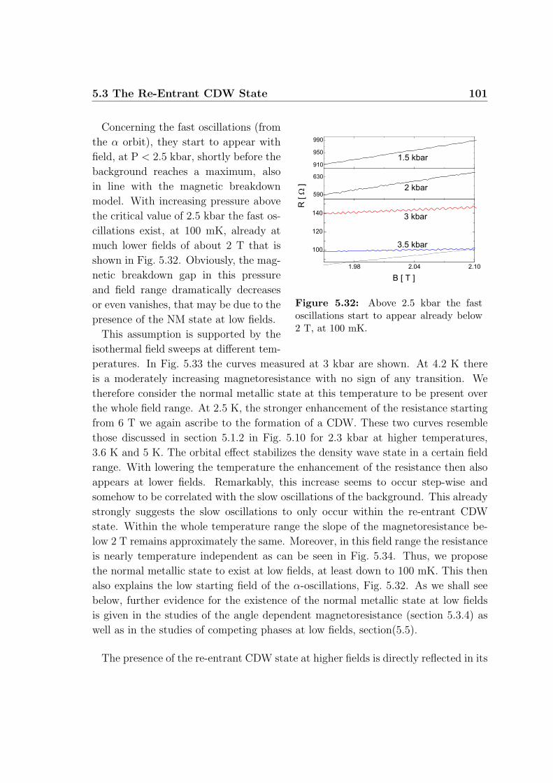
5.3 The Re-Entrant CDW State 101
Figure 5.32: Above 2.5 kbar the fastoscillations start to appear already below2 T, at 100 mK.
Concerning the fast oscillations (from
the α orbit), they start to appear with
field, at P < 2.5 kbar, shortly before the
background reaches a maximum, also
in line with the magnetic breakdown
model. With increasing pressure above
the critical value of 2.5 kbar the fast os-
cillations exist, at 100 mK, already at
much lower fields of about 2 T that is
shown in Fig. 5.32. Obviously, the mag-
netic breakdown gap in this pressure
and field range dramatically decreases
or even vanishes, that may be due to the
presence of the NM state at low fields.
This assumption is supported by the
isothermal field sweeps at different tem-
peratures. In Fig. 5.33 the curves measured at 3 kbar are shown. At 4.2 K there
is a moderately increasing magnetoresistance with no sign of any transition. We
therefore consider the normal metallic state at this temperature to be present over
the whole field range. At 2.5 K, the stronger enhancement of the resistance starting
from 6 T we again ascribe to the formation of a CDW. These two curves resemble
those discussed in section 5.1.2 in Fig. 5.10 for 2.3 kbar at higher temperatures,
3.6 K and 5 K. The orbital effect stabilizes the density wave state in a certain field
range. With lowering the temperature the enhancement of the resistance then also
appears at lower fields. Remarkably, this increase seems to occur step-wise and
somehow to be correlated with the slow oscillations of the background. This already
strongly suggests the slow oscillations to only occur within the re-entrant CDW
state. Within the whole temperature range the slope of the magnetoresistance be-
low 2 T remains approximately the same. Moreover, in this field range the resistance
is nearly temperature independent as can be seen in Fig. 5.34. Thus, we propose
the normal metallic state to exist at low fields, at least down to 100 mK. This then
also explains the low starting field of the α-oscillations, Fig. 5.32. As we shall see
below, further evidence for the existence of the normal metallic state at low fields
is given in the studies of the angle dependent magnetoresistance (section 5.3.4) as
well as in the studies of competing phases at low fields, section(5.5).
The presence of the re-entrant CDW state at higher fields is directly reflected in its
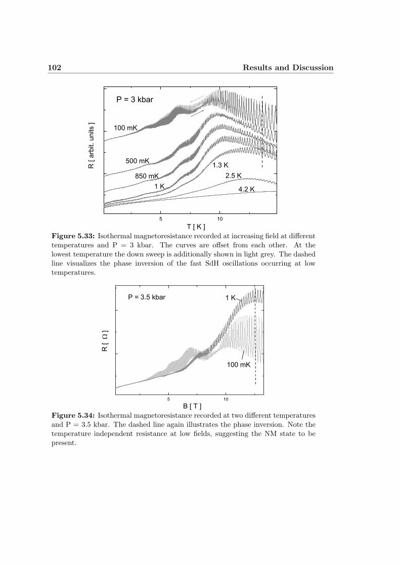
102 Results and Discussion
Figure 5.33: Isothermal magnetoresistance recorded at increasing field at differenttemperatures and P = 3 kbar. The curves are offset from each other. At thelowest temperature the down sweep is additionally shown in light grey. The dashedline visualizes the phase inversion of the fast SdH oscillations occurring at lowtemperatures.
Figure 5.34: Isothermal magnetoresistance recorded at two different temperaturesand P = 3.5 kbar. The dashed line again illustrates the phase inversion. Note thetemperature independent resistance at low fields, suggesting the NM state to bepresent.
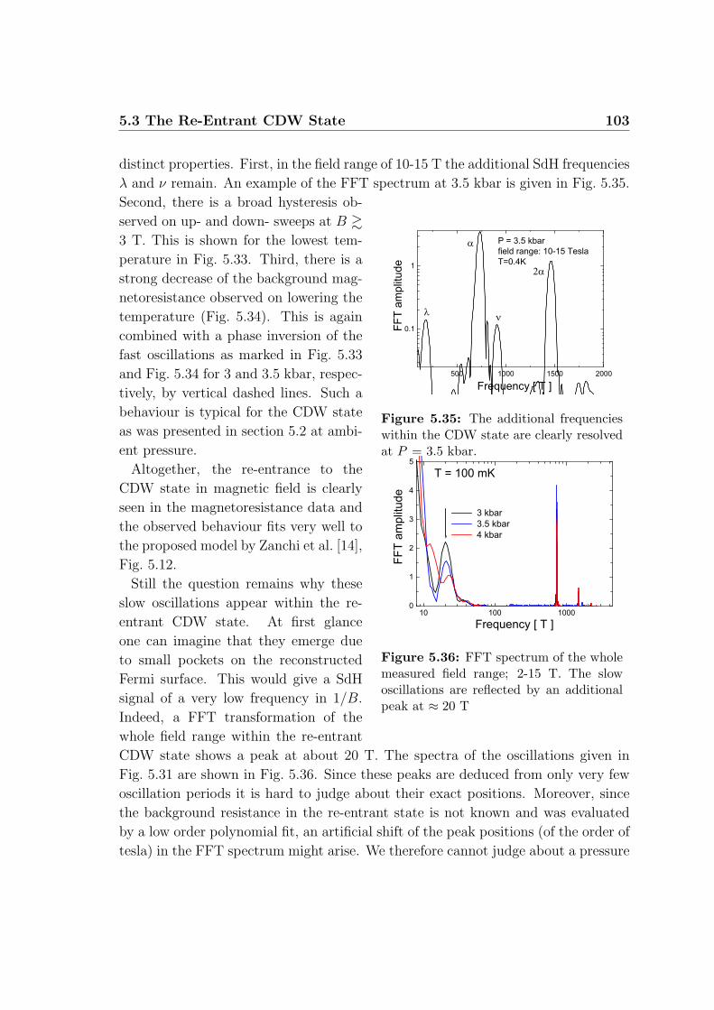
5.3 The Re-Entrant CDW State 103
distinct properties. First, in the field range of 10-15 T the additional SdH frequencies
λ and ν remain. An example of the FFT spectrum at 3.5 kbar is given in Fig. 5.35.
Figure 5.35: The additional frequencieswithin the CDW state are clearly resolvedat P = 3.5 kbar.
Figure 5.36: FFT spectrum of the wholemeasured field range; 2-15 T. The slowoscillations are reflected by an additionalpeak at ≈ 20 T
Second, there is a broad hysteresis ob-
served on up- and down- sweeps at B &3 T. This is shown for the lowest tem-
perature in Fig. 5.33. Third, there is a
strong decrease of the background mag-
netoresistance observed on lowering the
temperature (Fig. 5.34). This is again
combined with a phase inversion of the
fast oscillations as marked in Fig. 5.33
and Fig. 5.34 for 3 and 3.5 kbar, respec-
tively, by vertical dashed lines. Such a
behaviour is typical for the CDW state
as was presented in section 5.2 at ambi-
ent pressure.
Altogether, the re-entrance to the
CDW state in magnetic field is clearly
seen in the magnetoresistance data and
the observed behaviour fits very well to
the proposed model by Zanchi et al. [14],
Fig. 5.12.
Still the question remains why these
slow oscillations appear within the re-
entrant CDW state. At first glance
one can imagine that they emerge due
to small pockets on the reconstructed
Fermi surface. This would give a SdH
signal of a very low frequency in 1/B.
Indeed, a FFT transformation of the
whole field range within the re-entrant
CDW state shows a peak at about 20 T. The spectra of the oscillations given in
Fig. 5.31 are shown in Fig. 5.36. Since these peaks are deduced from only very few
oscillation periods it is hard to judge about their exact positions. Moreover, since
the background resistance in the re-entrant state is not known and was evaluated
by a low order polynomial fit, an artificial shift of the peak positions (of the order of
tesla) in the FFT spectrum might arise. We therefore cannot judge about a pressure
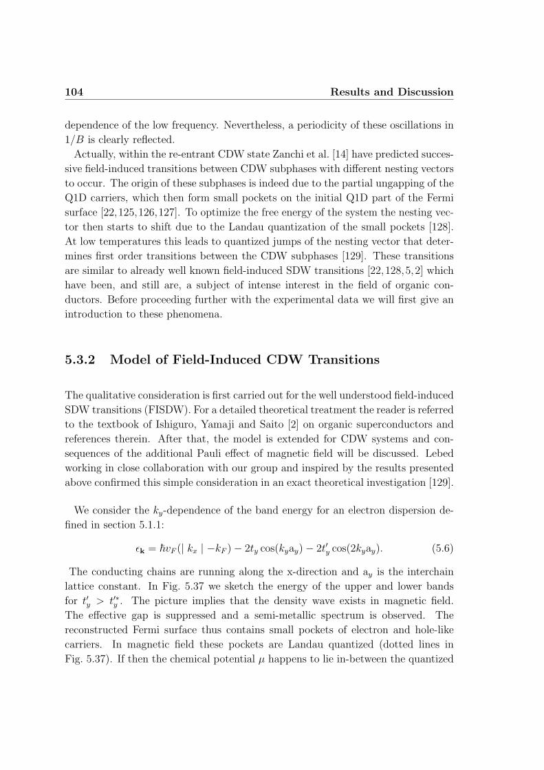
104 Results and Discussion
dependence of the low frequency. Nevertheless, a periodicity of these oscillations in
1/B is clearly reflected.
Actually, within the re-entrant CDW state Zanchi et al. [14] have predicted succes-
sive field-induced transitions between CDW subphases with different nesting vectors
to occur. The origin of these subphases is indeed due to the partial ungapping of the
Q1D carriers, which then form small pockets on the initial Q1D part of the Fermi
surface [22,125,126,127]. To optimize the free energy of the system the nesting vec-
tor then starts to shift due to the Landau quantization of the small pockets [128].
At low temperatures this leads to quantized jumps of the nesting vector that deter-
mines first order transitions between the CDW subphases [129]. These transitions
are similar to already well known field-induced SDW transitions [22,128,5,2] which
have been, and still are, a subject of intense interest in the field of organic con-
ductors. Before proceeding further with the experimental data we will first give an
introduction to these phenomena.
5.3.2 Model of Field-Induced CDW Transitions
The qualitative consideration is first carried out for the well understood field-induced
SDW transitions (FISDW). For a detailed theoretical treatment the reader is referred
to the textbook of Ishiguro, Yamaji and Saito [2] on organic superconductors and
references therein. After that, the model is extended for CDW systems and con-
sequences of the additional Pauli effect of magnetic field will be discussed. Lebed
working in close collaboration with our group and inspired by the results presented
above confirmed this simple consideration in an exact theoretical investigation [129].
We consider the ky-dependence of the band energy for an electron dispersion de-
fined in section 5.1.1:
εk = ~vF (| kx | −kF )− 2ty cos(kyay)− 2t′y cos(2kyay). (5.6)
The conducting chains are running along the x-direction and ay is the interchain
lattice constant. In Fig. 5.37 we sketch the energy of the upper and lower bands
for t′y > t′∗y . The picture implies that the density wave exists in magnetic field.
The effective gap is suppressed and a semi-metallic spectrum is observed. The
reconstructed Fermi surface thus contains small pockets of electron and hole-like
carriers. In magnetic field these pockets are Landau quantized (dotted lines in
Fig. 5.37). If then the chemical potential µ happens to lie in-between the quantized
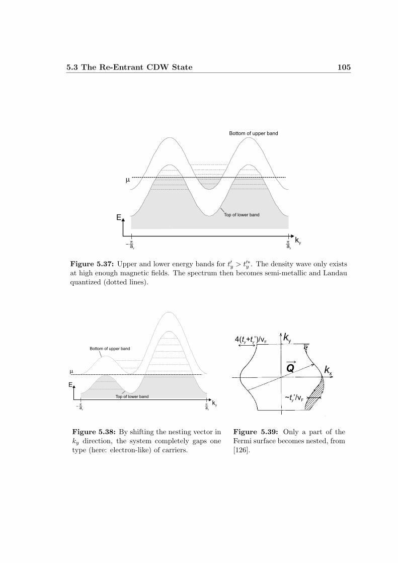
5.3 The Re-Entrant CDW State 105
m
Top of lower band
Bottom of upper band
E
kyp
ay
p
ay
Figure 5.37: Upper and lower energy bands for t′y > t′∗y . The density wave only existsat high enough magnetic fields. The spectrum then becomes semi-metallic and Landauquantized (dotted lines).
kyp
ay
m
E
p
ay
Bottom of upper band
Top of lower band
Figure 5.38: By shifting the nesting vector inky direction, the system completely gaps onetype (here: electron-like) of carriers.
ky
kx
~ ’/vty F
4( ’)/vt +ty y F
Q
Figure 5.39: Only a part of theFermi surface becomes nested, from[126].
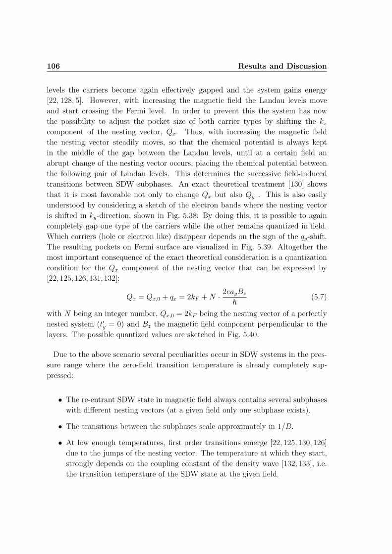
106 Results and Discussion
levels the carriers become again effectively gapped and the system gains energy
[22, 128, 5]. However, with increasing the magnetic field the Landau levels move
and start crossing the Fermi level. In order to prevent this the system has now
the possibility to adjust the pocket size of both carrier types by shifting the kx
component of the nesting vector, Qx. Thus, with increasing the magnetic field
the nesting vector steadily moves, so that the chemical potential is always kept
in the middle of the gap between the Landau levels, until at a certain field an
abrupt change of the nesting vector occurs, placing the chemical potential between
the following pair of Landau levels. This determines the successive field-induced
transitions between SDW subphases. An exact theoretical treatment [130] shows
that it is most favorable not only to change Qx but also Qy . This is also easily
understood by considering a sketch of the electron bands where the nesting vector
is shifted in ky-direction, shown in Fig. 5.38: By doing this, it is possible to again
completely gap one type of the carriers while the other remains quantized in field.
Which carriers (hole or electron like) disappear depends on the sign of the qy-shift.
The resulting pockets on Fermi surface are visualized in Fig. 5.39. Altogether the
most important consequence of the exact theoretical consideration is a quantization
condition for the Qx component of the nesting vector that can be expressed by
[22,125,126,131,132]:
Qx = Qx,0 + qx = 2kF + N · 2eayBz
~(5.7)
with N being an integer number, Qx,0 = 2kF being the nesting vector of a perfectly
nested system (t′y = 0) and Bz the magnetic field component perpendicular to the
layers. The possible quantized values are sketched in Fig. 5.40.
Due to the above scenario several peculiarities occur in SDW systems in the pres-
sure range where the zero-field transition temperature is already completely sup-
pressed:
• The re-entrant SDW state in magnetic field always contains several subphases
with different nesting vectors (at a given field only one subphase exists).
• The transitions between the subphases scale approximately in 1/B.
• At low enough temperatures, first order transitions emerge [22, 125, 130, 126]
due to the jumps of the nesting vector. The temperature at which they start,
strongly depends on the coupling constant of the density wave [132, 133], i.e.
the transition temperature of the SDW state at the given field.
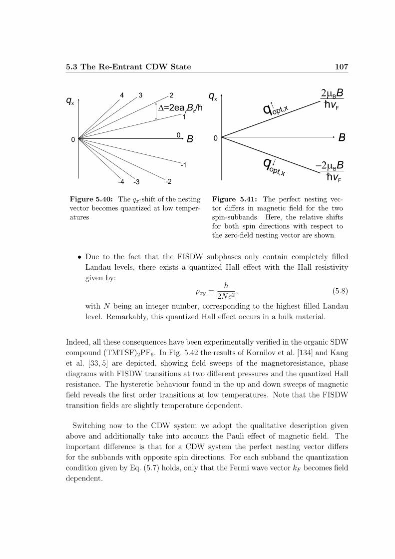
5.3 The Re-Entrant CDW State 107
qx
-3 -2
-1
1
234
0
-4
B
D=2ea /hy zB
0
Figure 5.40: The qx-shift of the nestingvector becomes quantized at low temper-atures
B
2mBBhvF
-2mBBhvF
B
qx
0
qopt,x
qopt,x
Figure 5.41: The perfect nesting vec-tor differs in magnetic field for the twospin-subbands. Here, the relative shiftsfor both spin directions with respect tothe zero-field nesting vector are shown.
• Due to the fact that the FISDW subphases only contain completely filled
Landau levels, there exists a quantized Hall effect with the Hall resistivity
given by:
ρxy =h
2Ne2, (5.8)
with N being an integer number, corresponding to the highest filled Landau
level. Remarkably, this quantized Hall effect occurs in a bulk material.
Indeed, all these consequences have been experimentally verified in the organic SDW
compound (TMTSF)2PF6. In Fig. 5.42 the results of Kornilov et al. [134] and Kang
et al. [33, 5] are depicted, showing field sweeps of the magnetoresistance, phase
diagrams with FISDW transitions at two different pressures and the quantized Hall
resistance. The hysteretic behaviour found in the up and down sweeps of magnetic
field reveals the first order transitions at low temperatures. Note that the FISDW
transition fields are slightly temperature dependent.
Switching now to the CDW system we adopt the qualitative description given
above and additionally take into account the Pauli effect of magnetic field. The
important difference is that for a CDW system the perfect nesting vector differs
for the subbands with opposite spin directions. For each subband the quantization
condition given by Eq. (5.7) holds, only that the Fermi wave vector kF becomes field
dependent.
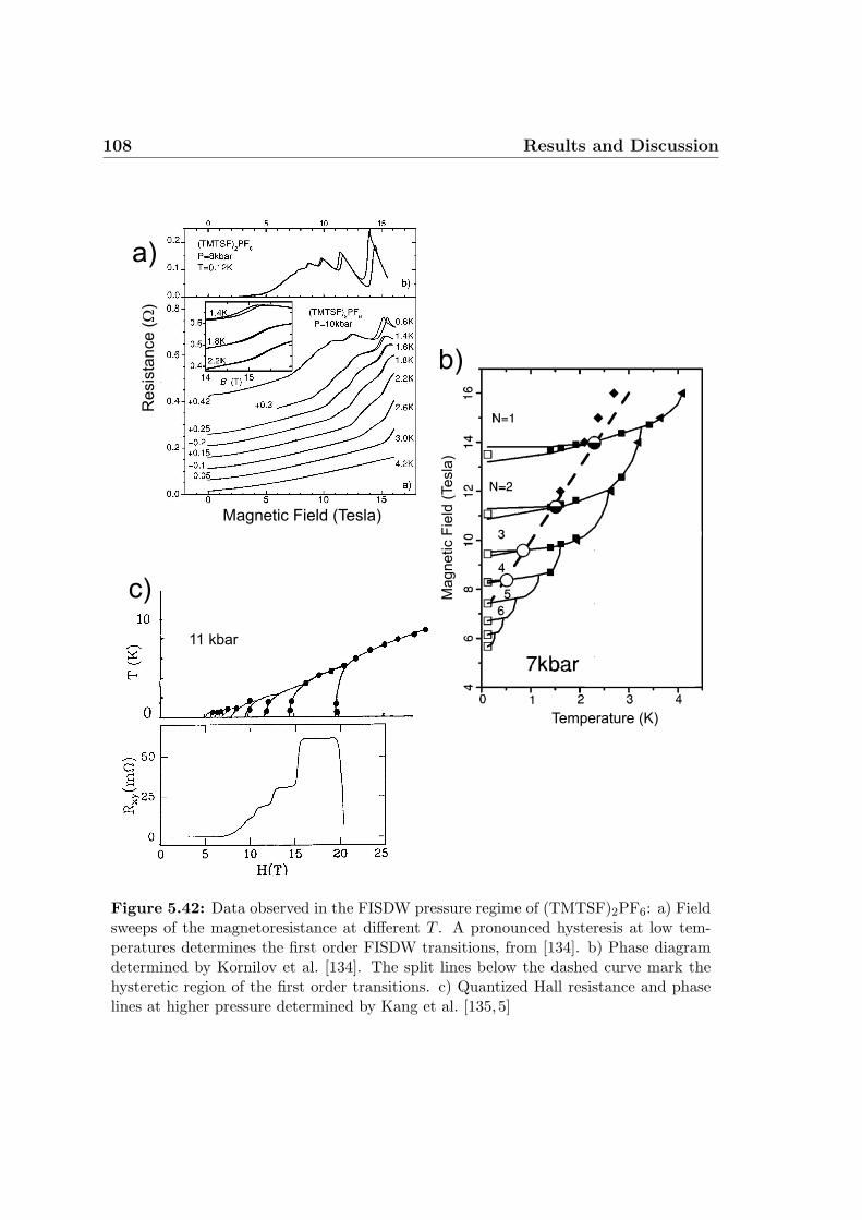
108 Results and Discussion
b)
Ma
gn
etic F
ield
(Te
sla
)
Temperature (K)
c)
11 kbar
Resis
tan
ce (
)W
a)
Magnetic Field (Tesla)
Figure 5.42: Data observed in the FISDW pressure regime of (TMTSF)2PF6: a) Fieldsweeps of the magnetoresistance at different T . A pronounced hysteresis at low tem-peratures determines the first order FISDW transitions, from [134]. b) Phase diagramdetermined by Kornilov et al. [134]. The split lines below the dashed curve mark thehysteretic region of the first order transitions. c) Quantized Hall resistance and phaselines at higher pressure determined by Kang et al. [135,5]
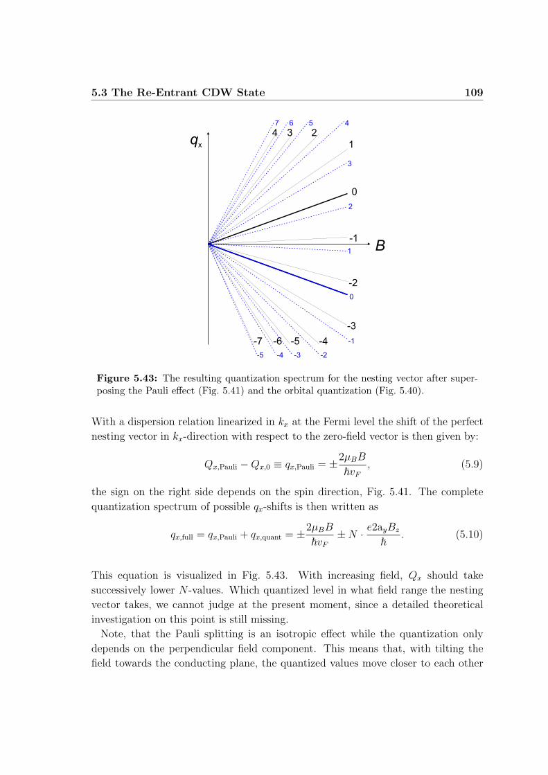
5.3 The Re-Entrant CDW State 109
1
-6
0
-1
-2
-3
-4-5
0
4 3 2
1
7
2
3
46 5
-4 -3 -2
-1-7
-5
qx
B
Figure 5.43: The resulting quantization spectrum for the nesting vector after super-posing the Pauli effect (Fig. 5.41) and the orbital quantization (Fig. 5.40).
With a dispersion relation linearized in kx at the Fermi level the shift of the perfect
nesting vector in kx-direction with respect to the zero-field vector is then given by:
Qx,Pauli −Qx,0 ≡ qx,Pauli = ±2µBB
~vF
, (5.9)
the sign on the right side depends on the spin direction, Fig. 5.41. The complete
quantization spectrum of possible qx-shifts is then written as
qx,full = qx,Pauli + qx,quant = ±2µBB
~vF
±N · e2ayBz
~. (5.10)
This equation is visualized in Fig. 5.43. With increasing field, Qx should take
successively lower N -values. Which quantized level in what field range the nesting
vector takes, we cannot judge at the present moment, since a detailed theoretical
investigation on this point is still missing.
Note, that the Pauli splitting is an isotropic effect while the quantization only
depends on the perpendicular field component. This means that, with tilting the
field towards the conducting plane, the quantized values move closer to each other
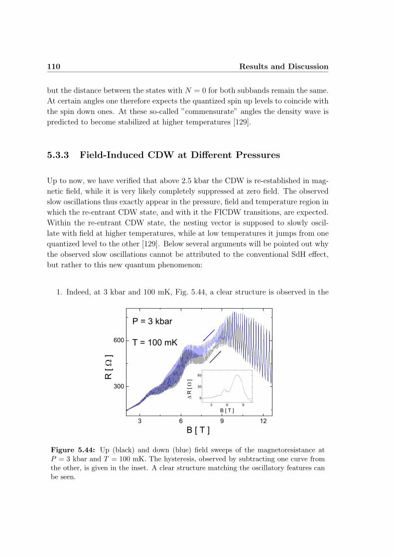
110 Results and Discussion
but the distance between the states with N = 0 for both subbands remain the same.
At certain angles one therefore expects the quantized spin up levels to coincide with
the spin down ones. At these so-called ”commensurate” angles the density wave is
predicted to become stabilized at higher temperatures [129].
5.3.3 Field-Induced CDW at Different Pressures
Up to now, we have verified that above 2.5 kbar the CDW is re-established in mag-
netic field, while it is very likely completely suppressed at zero field. The observed
slow oscillations thus exactly appear in the pressure, field and temperature region in
which the re-entrant CDW state, and with it the FICDW transitions, are expected.
Within the re-entrant CDW state, the nesting vector is supposed to slowly oscil-
late with field at higher temperatures, while at low temperatures it jumps from one
quantized level to the other [129]. Below several arguments will be pointed out why
the observed slow oscillations cannot be attributed to the conventional SdH effect,
but rather to this new quantum phenomenon:
1. Indeed, at 3 kbar and 100 mK, Fig. 5.44, a clear structure is observed in the
Figure 5.44: Up (black) and down (blue) field sweeps of the magnetoresistance atP = 3 kbar and T = 100 mK. The hysteresis, observed by subtracting one curve fromthe other, is given in the inset. A clear structure matching the oscillatory features canbe seen.
5.3 The Re-Entrant CDW State 111
hysteresis in the up and down field sweeps that correlates with the slow oscil-
lations. To determine the hysteresis, the fast oscillations were filtered out from
these curves. As can be seen in the inset of Fig. 5.44 the hysteresis exhibits
clear maxima at approximately the field positions where the background mag-
netoresistance has a maximum curvature with respect to magnetic field. This
observation we regard as the first sign for the expected first order transitions
between the subphases. Unfortunately, our cooling system did not allow us to
go to even lower temperature on ramping to such high magnetic fields, so that
this is the only clear hysteretic structure observed in our measurement at the
perpendicular field direction. Unlike the sharp hysteretic transitions seen at
the FISDW transitions, Fig. 5.42, the peaks in our compound are very broad.
Obviously, the first order transitions start to appear at much lower tempera-
ture (with respect to the re-entrant CDW transition temperature at a given
field) in comparison to the FISDW case. This, however, should be expected,
since in FICDW the quantized values of the nesting vector for different spin
directions at perpendicular magnetic field likely do not match each other. This
will directly lead to a lower coupling constant and, hence,to a lower transition
temperature of the re-entrant CDW as well as a lower starting temperature of
the first order transitions [129].
2. Another peculiarity of the slow oscillations is shown in Fig. 5.45. On lowering
the temperature it is obvious that the phase of the oscillations is temper-
ature dependent. To illustrate this, dashed lines are placed into Fig. 5.45
approximately following the maximum curvature of the slow oscillations. This
anomalous behaviour is certainly not expected for normal quantum oscillations
and to the moment we attribute this finding to the new quantum phenomenon
of FICDW transitions.
In analogy to the FISDW, we now determine B-T phase diagrams for the
present FICDW case. To extract transition points between different CDW
subphases from the background magnetoresistance the fast oscillations have
been filtered out as shown in Fig. 5.45. As a transition field we choose the
points of maximum curvature in the field sweeps, since (i) they coincide very
well with the observed peaks in the hysteresis (Fig. 5.44) and (ii) are rea-
sonable if one expects a change of the nesting vector to improve the nesting
conditions, and with it to enhance the magnetoresistance. We therefore as-
sume the real transition fields to behave in a similar manner as the extracted
points. Fig. 5.46 shows the observed phase diagrams in the re-entrant CDW
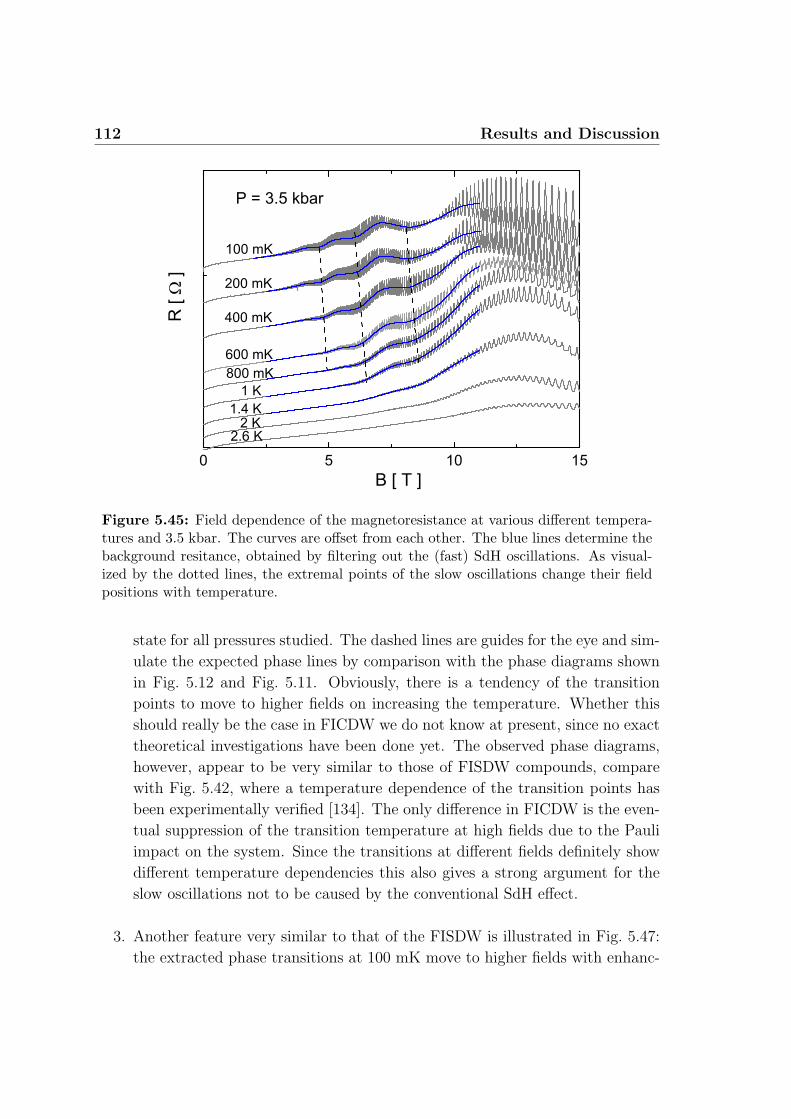
112 Results and Discussion
Figure 5.45: Field dependence of the magnetoresistance at various different tempera-tures and 3.5 kbar. The curves are offset from each other. The blue lines determine thebackground resitance, obtained by filtering out the (fast) SdH oscillations. As visual-ized by the dotted lines, the extremal points of the slow oscillations change their fieldpositions with temperature.
state for all pressures studied. The dashed lines are guides for the eye and sim-
ulate the expected phase lines by comparison with the phase diagrams shown
in Fig. 5.12 and Fig. 5.11. Obviously, there is a tendency of the transition
points to move to higher fields on increasing the temperature. Whether this
should really be the case in FICDW we do not know at present, since no exact
theoretical investigations have been done yet. The observed phase diagrams,
however, appear to be very similar to those of FISDW compounds, compare
with Fig. 5.42, where a temperature dependence of the transition points has
been experimentally verified [134]. The only difference in FICDW is the even-
tual suppression of the transition temperature at high fields due to the Pauli
impact on the system. Since the transitions at different fields definitely show
different temperature dependencies this also gives a strong argument for the
slow oscillations not to be caused by the conventional SdH effect.
3. Another feature very similar to that of the FISDW is illustrated in Fig. 5.47:
the extracted phase transitions at 100 mK move to higher fields with enhanc-
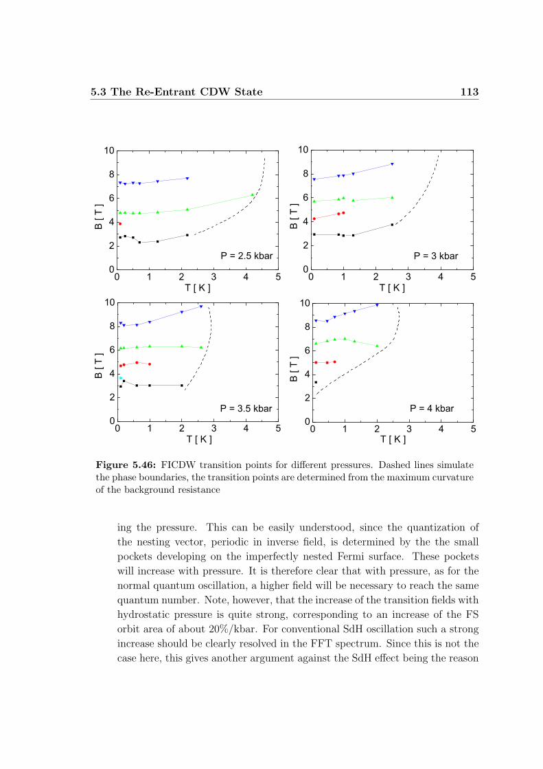
5.3 The Re-Entrant CDW State 113
Figure 5.46: FICDW transition points for different pressures. Dashed lines simulatethe phase boundaries, the transition points are determined from the maximum curvatureof the background resistance
ing the pressure. This can be easily understood, since the quantization of
the nesting vector, periodic in inverse field, is determined by the the small
pockets developing on the imperfectly nested Fermi surface. These pockets
will increase with pressure. It is therefore clear that with pressure, as for the
normal quantum oscillation, a higher field will be necessary to reach the same
quantum number. Note, however, that the increase of the transition fields with
hydrostatic pressure is quite strong, corresponding to an increase of the FS
orbit area of about 20%/kbar. For conventional SdH oscillation such a strong
increase should be clearly resolved in the FFT spectrum. Since this is not the
case here, this gives another argument against the SdH effect being the reason
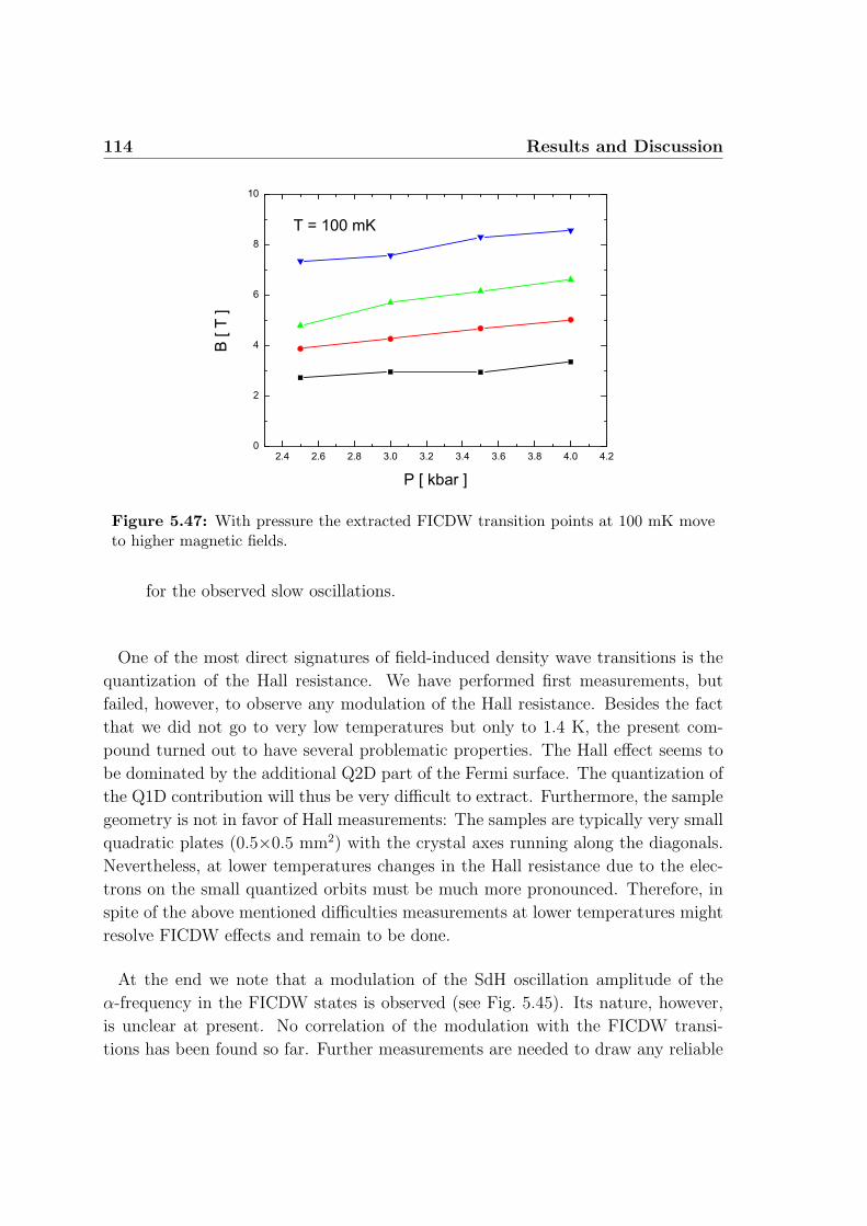
114 Results and Discussion
Figure 5.47: With pressure the extracted FICDW transition points at 100 mK moveto higher magnetic fields.
for the observed slow oscillations.
One of the most direct signatures of field-induced density wave transitions is the
quantization of the Hall resistance. We have performed first measurements, but
failed, however, to observe any modulation of the Hall resistance. Besides the fact
that we did not go to very low temperatures but only to 1.4 K, the present com-
pound turned out to have several problematic properties. The Hall effect seems to
be dominated by the additional Q2D part of the Fermi surface. The quantization of
the Q1D contribution will thus be very difficult to extract. Furthermore, the sample
geometry is not in favor of Hall measurements: The samples are typically very small
quadratic plates (0.5×0.5 mm2) with the crystal axes running along the diagonals.
Nevertheless, at lower temperatures changes in the Hall resistance due to the elec-
trons on the small quantized orbits must be much more pronounced. Therefore, in
spite of the above mentioned difficulties measurements at lower temperatures might
resolve FICDW effects and remain to be done.
At the end we note that a modulation of the SdH oscillation amplitude of the
α-frequency in the FICDW states is observed (see Fig. 5.45). Its nature, however,
is unclear at present. No correlation of the modulation with the FICDW transi-
tions has been found so far. Further measurements are needed to draw any reliable
5.3 The Re-Entrant CDW State 115
conclusions.
5.3.4 Angle Dependent Magnetoresistance
In view of the results, presented up to now within this section, there are two main
reasons for studying the angle dependent magnetoresistance.
The first one emerges due to the present transition from the NM state to the
re-entrant CDW state in magnetic field at P & P0. This transition might also
be reflected in AMRO measurements. At ambient pressure the AMROs in the
CDW state are known to strongly differ from the ones in the NM state: while the
former are typical of a Q1D electron system the latter show the Q2D behaviour
(see section 3.4). Since we have seen that within the re-entrant CDW state the
semiclassical magnetoresistance is still remarkably high over a wide field range, one
can expect signs of the 1D AMROs to occur.
The second reason concerns the field-induced density wave transitions in magnetic
field. As mentioned above the orbital quantization only depends on the magnetic
field component perpendicular to the layer, Bz. On the other hand the Pauli effect
is known to be isotropic. Hence, on tilting the field there must be certain ”commen-
surate” directions at which the quantized levels of the nesting vector for the spin up
and spin down bands match each other (the quantum numbers of the different bands
always being different). At such angles one thus expects optimal conditions for the
FICDW transitions. Indeed, Lebed predicted that at these commensurate angles
both the transition temperature of the re-entrant CDW at a given field and the
starting temperature of the first order transitions with field must become enhanced.
In addition, a ”peak-effect” can be expected in the AMRO at these commensurate
angles, since there the CDW is stabilized already at higher temperatures.
For these measurements a small pressure cell was mounted on the newly con-
structed two axes rotation insert, which allowed the sample to be cooled down to
0.4 K in a 3He cooling system. For continuous rotation at a reasonable speed, nec-
essary for AMRO measurements, the lowest possible temperature was 0.7 K. The
definition of the angles θ and ϕ of the sample position with respect to the field is
depicted in Fig. 5.48.
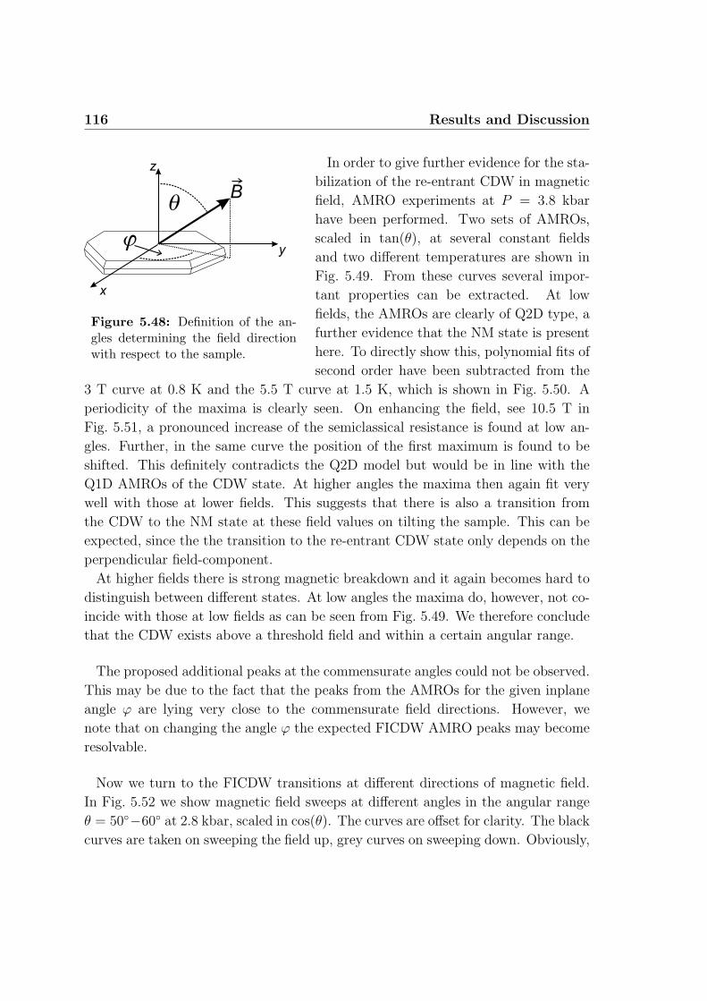
116 Results and Discussion
j
q
z
x
y
B
Figure 5.48: Definition of the an-gles determining the field directionwith respect to the sample.
In order to give further evidence for the sta-
bilization of the re-entrant CDW in magnetic
field, AMRO experiments at P = 3.8 kbar
have been performed. Two sets of AMROs,
scaled in tan(θ), at several constant fields
and two different temperatures are shown in
Fig. 5.49. From these curves several impor-
tant properties can be extracted. At low
fields, the AMROs are clearly of Q2D type, a
further evidence that the NM state is present
here. To directly show this, polynomial fits of
second order have been subtracted from the
3 T curve at 0.8 K and the 5.5 T curve at 1.5 K, which is shown in Fig. 5.50. A
periodicity of the maxima is clearly seen. On enhancing the field, see 10.5 T in
Fig. 5.51, a pronounced increase of the semiclassical resistance is found at low an-
gles. Further, in the same curve the position of the first maximum is found to be
shifted. This definitely contradicts the Q2D model but would be in line with the
Q1D AMROs of the CDW state. At higher angles the maxima then again fit very
well with those at lower fields. This suggests that there is also a transition from
the CDW to the NM state at these field values on tilting the sample. This can be
expected, since the the transition to the re-entrant CDW state only depends on the
perpendicular field-component.
At higher fields there is strong magnetic breakdown and it again becomes hard to
distinguish between different states. At low angles the maxima do, however, not co-
incide with those at low fields as can be seen from Fig. 5.49. We therefore conclude
that the CDW exists above a threshold field and within a certain angular range.
The proposed additional peaks at the commensurate angles could not be observed.
This may be due to the fact that the peaks from the AMROs for the given inplane
angle ϕ are lying very close to the commensurate field directions. However, we
note that on changing the angle ϕ the expected FICDW AMRO peaks may become
resolvable.
Now we turn to the FICDW transitions at different directions of magnetic field.
In Fig. 5.52 we show magnetic field sweeps at different angles in the angular range
θ = 50−60 at 2.8 kbar, scaled in cos(θ). The curves are offset for clarity. The black
curves are taken on sweeping the field up, grey curves on sweeping down. Obviously,
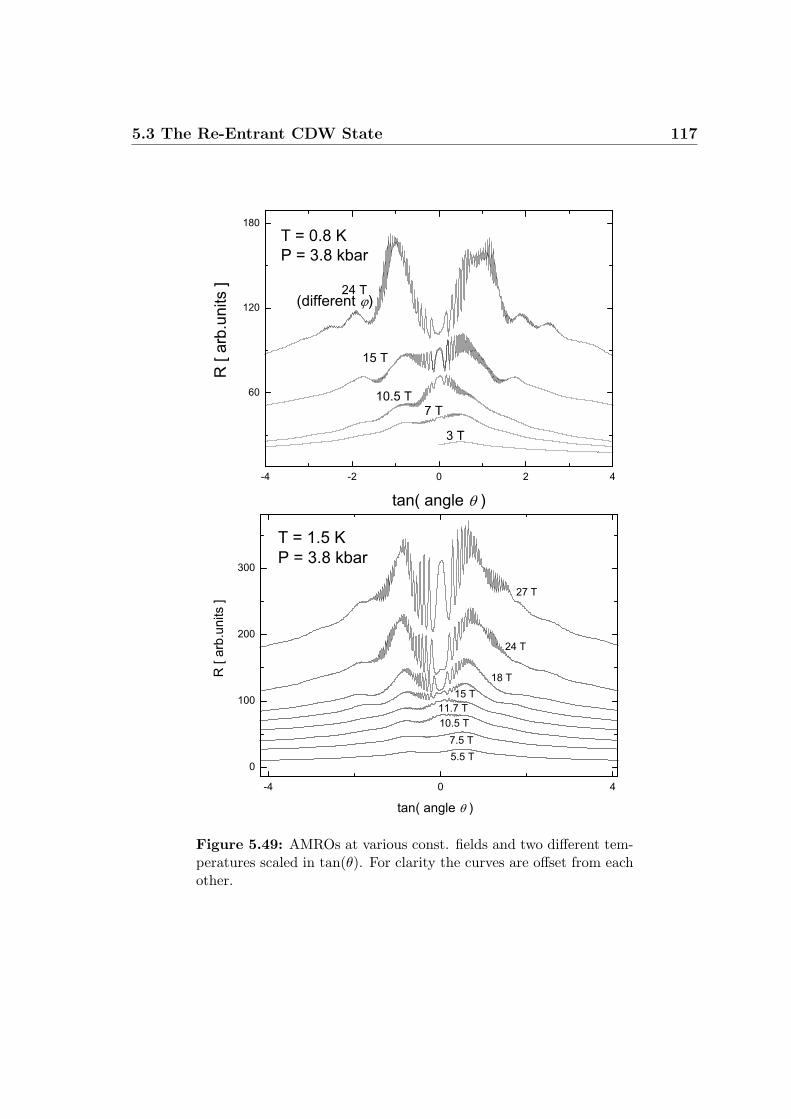
5.3 The Re-Entrant CDW State 117
Figure 5.49: AMROs at various const. fields and two different tem-peratures scaled in tan(θ). For clarity the curves are offset from eachother.
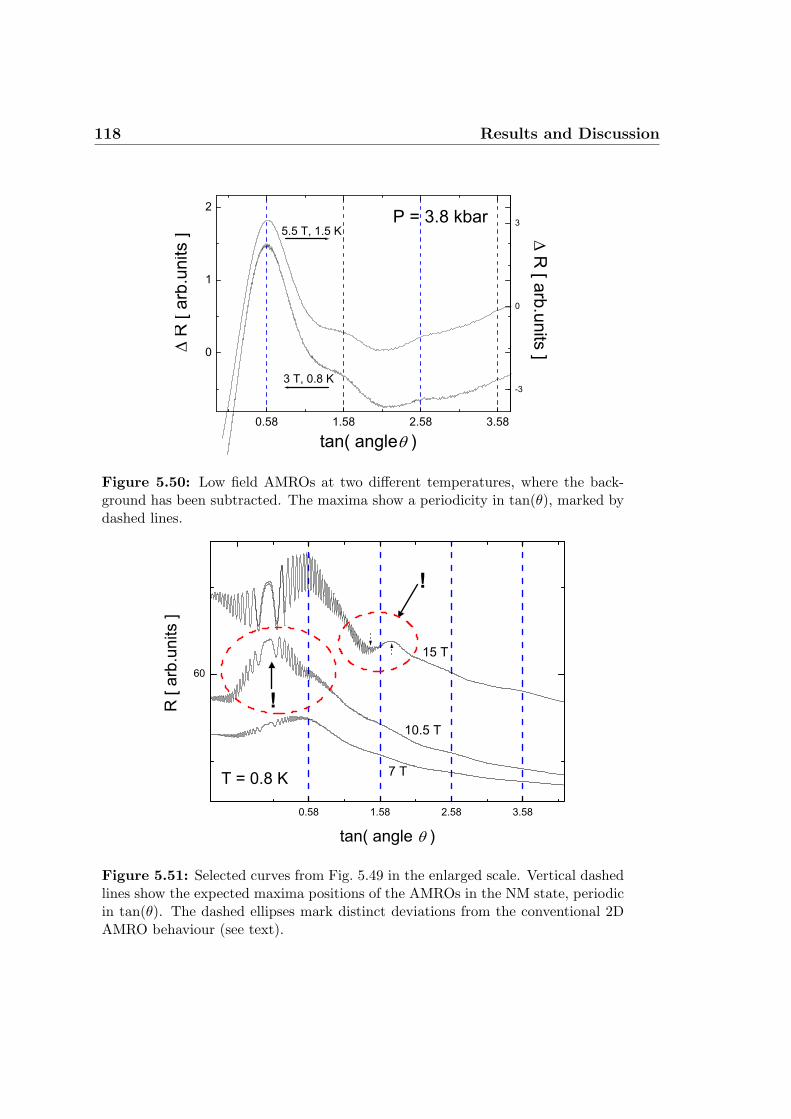
118 Results and Discussion
Figure 5.50: Low field AMROs at two different temperatures, where the back-ground has been subtracted. The maxima show a periodicity in tan(θ), marked bydashed lines.
Figure 5.51: Selected curves from Fig. 5.49 in the enlarged scale. Vertical dashedlines show the expected maxima positions of the AMROs in the NM state, periodicin tan(θ). The dashed ellipses mark distinct deviations from the conventional 2DAMRO behaviour (see text).
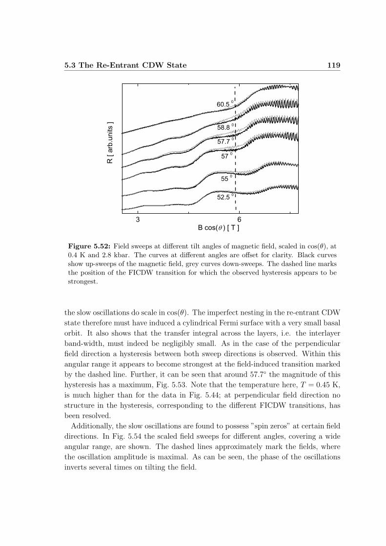
5.3 The Re-Entrant CDW State 119
Figure 5.52: Field sweeps at different tilt angles of magnetic field, scaled in cos(θ), at0.4 K and 2.8 kbar. The curves at different angles are offset for clarity. Black curvesshow up-sweeps of the magnetic field, grey curves down-sweeps. The dashed line marksthe position of the FICDW transition for which the observed hysteresis appears to bestrongest.
the slow oscillations do scale in cos(θ). The imperfect nesting in the re-entrant CDW
state therefore must have induced a cylindrical Fermi surface with a very small basal
orbit. It also shows that the transfer integral across the layers, i.e. the interlayer
band-width, must indeed be negligibly small. As in the case of the perpendicular
field direction a hysteresis between both sweep directions is observed. Within this
angular range it appears to become strongest at the field-induced transition marked
by the dashed line. Further, it can be seen that around 57.7 the magnitude of this
hysteresis has a maximum, Fig. 5.53. Note that the temperature here, T = 0.45 K,
is much higher than for the data in Fig. 5.44; at perpendicular field direction no
structure in the hysteresis, corresponding to the different FICDW transitions, has
been resolved.
Additionally, the slow oscillations are found to possess ”spin zeros” at certain field
directions. In Fig. 5.54 the scaled field sweeps for different angles, covering a wide
angular range, are shown. The dashed lines approximately mark the fields, where
the oscillation amplitude is maximal. As can be seen, the phase of the oscillations
inverts several times on tilting the field.
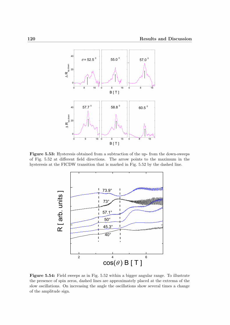
120 Results and Discussion
Figure 5.53: Hysteresis obtained from a subtraction of the up- from the down-sweepsof Fig. 5.52 at different field directions. The arrow points to the maximum in thehysteresis at the FICDW transition that is marked in Fig. 5.52 by the dashed line.
Figure 5.54: Field sweeps as in Fig. 5.52 within a bigger angular range. To illustratethe presence of spin zeros, dashed lines are approximately placed at the extrema of theslow oscillations. On increasing the angle the oscillations show several times a changeof the amplitude sign.
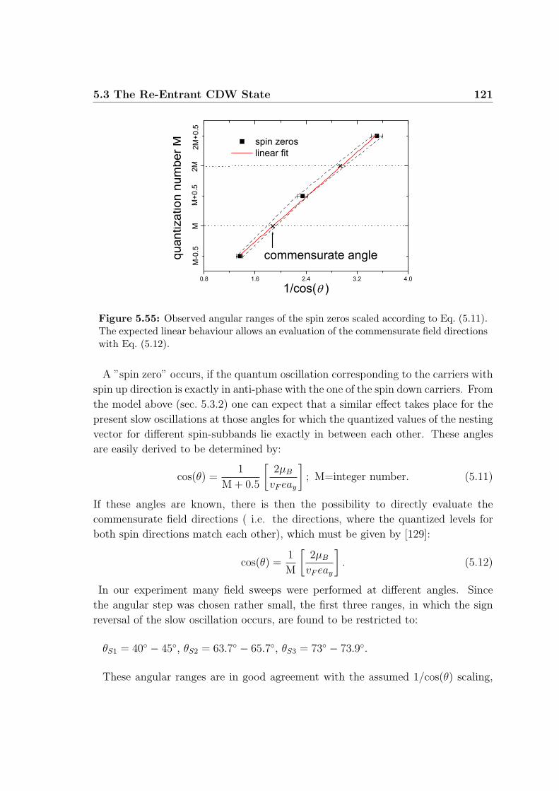
5.3 The Re-Entrant CDW State 121
Figure 5.55: Observed angular ranges of the spin zeros scaled according to Eq. (5.11).The expected linear behaviour allows an evaluation of the commensurate field directionswith Eq. (5.12).
A ”spin zero” occurs, if the quantum oscillation corresponding to the carriers with
spin up direction is exactly in anti-phase with the one of the spin down carriers. From
the model above (sec. 5.3.2) one can expect that a similar effect takes place for the
present slow oscillations at those angles for which the quantized values of the nesting
vector for different spin-subbands lie exactly in between each other. These angles
are easily derived to be determined by:
cos(θ) =1
M + 0.5
[2µB
vF eay
]; M=integer number. (5.11)
If these angles are known, there is then the possibility to directly evaluate the
commensurate field directions ( i.e. the directions, where the quantized levels for
both spin directions match each other), which must be given by [129]:
cos(θ) =1
M
[2µB
vF eay
]. (5.12)
In our experiment many field sweeps were performed at different angles. Since
the angular step was chosen rather small, the first three ranges, in which the sign
reversal of the slow oscillation occurs, are found to be restricted to:
θS1 = 40 − 45, θS2 = 63.7 − 65.7, θS3 = 73 − 73.9.
These angular ranges are in good agreement with the assumed 1/cos(θ) scaling,
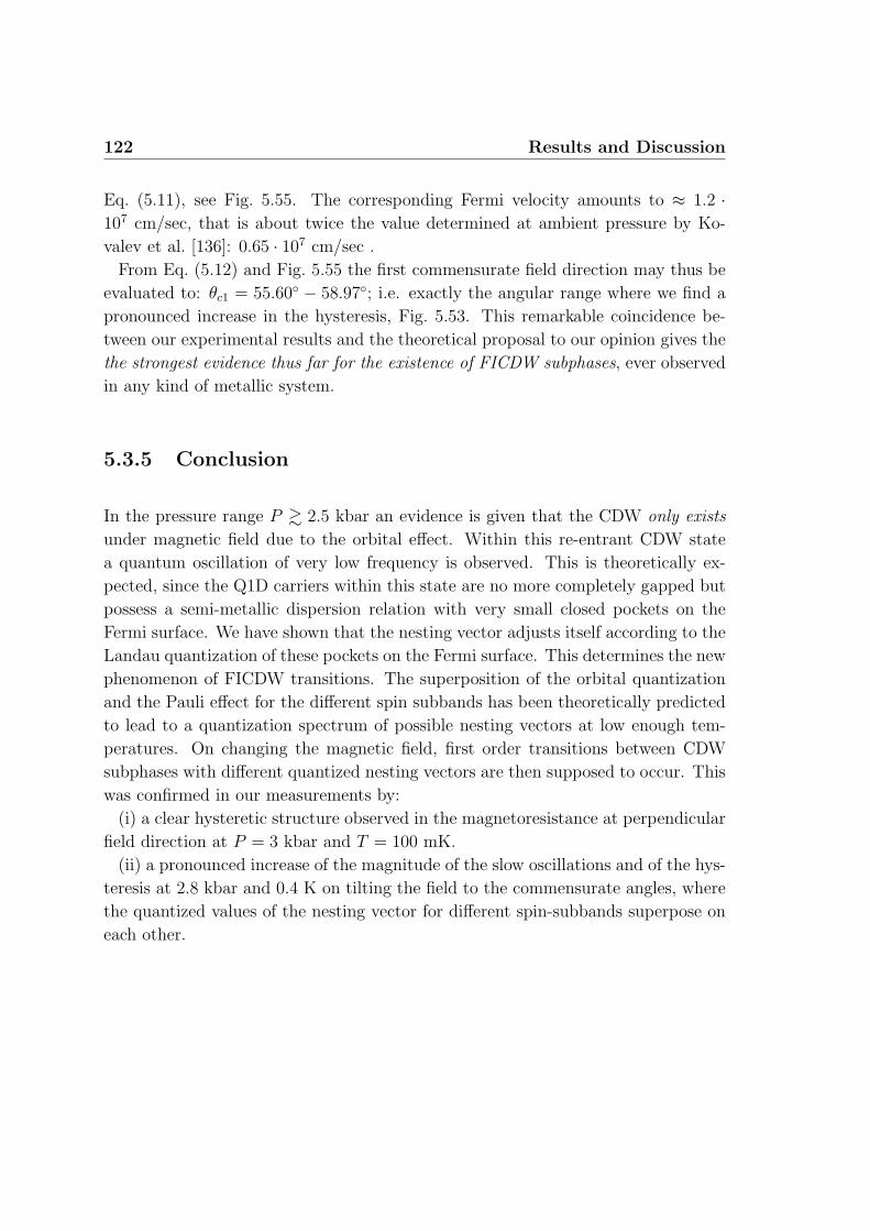
122 Results and Discussion
Eq. (5.11), see Fig. 5.55. The corresponding Fermi velocity amounts to ≈ 1.2 ·107 cm/sec, that is about twice the value determined at ambient pressure by Ko-
valev et al. [136]: 0.65 · 107 cm/sec .
From Eq. (5.12) and Fig. 5.55 the first commensurate field direction may thus be
evaluated to: θc1 = 55.60 − 58.97; i.e. exactly the angular range where we find a
pronounced increase in the hysteresis, Fig. 5.53. This remarkable coincidence be-
tween our experimental results and the theoretical proposal to our opinion gives the
the strongest evidence thus far for the existence of FICDW subphases, ever observed
in any kind of metallic system.
5.3.5 Conclusion
In the pressure range P & 2.5 kbar an evidence is given that the CDW only exists
under magnetic field due to the orbital effect. Within this re-entrant CDW state
a quantum oscillation of very low frequency is observed. This is theoretically ex-
pected, since the Q1D carriers within this state are no more completely gapped but
possess a semi-metallic dispersion relation with very small closed pockets on the
Fermi surface. We have shown that the nesting vector adjusts itself according to the
Landau quantization of these pockets on the Fermi surface. This determines the new
phenomenon of FICDW transitions. The superposition of the orbital quantization
and the Pauli effect for the different spin subbands has been theoretically predicted
to lead to a quantization spectrum of possible nesting vectors at low enough tem-
peratures. On changing the magnetic field, first order transitions between CDW
subphases with different quantized nesting vectors are then supposed to occur. This
was confirmed in our measurements by:
(i) a clear hysteretic structure observed in the magnetoresistance at perpendicular
field direction at P = 3 kbar and T = 100 mK.
(ii) a pronounced increase of the magnitude of the slow oscillations and of the hys-
teresis at 2.8 kbar and 0.4 K on tilting the field to the commensurate angles, where
the quantized values of the nesting vector for different spin-subbands superpose on
each other.
5.4 Field-Induced CDW Transitions at High Tilt Angles 123
5.4 Field-Induced CDW Transitions at High Tilt
Angles
5.4.1 Magnetic Torque and Magnetoresistance at Ambient
Pressure
So far the ambient pressure B-T phase diagram has been considered under a mag-
netic field applied approximately perpendicular to the highly conducting a-c plane.
We now investigate changes occurring at ambient pressure on tilting the field to-
wards the plane. Basically, one can expect orbital effects to become strongly reduced
at high tilt angles, since their strength depends solely on the field component per-
pendicular to the layers. If, for instance, the CDW state at ambient pressure is not
perfectly nested, a reduction of the orbital effect will change the B-T phase dia-
gram: The low field CDW state becomes suppressed, and therefore the CDWx state
stabilized, already at lower fields.5 The observed changes on tilting the sample are,
however, known to be far more complex. At high tilt angles the magnetic torque as
well as the interlayer magnetoresistance exhibit several anomalies in the isothermal
field sweeps at low temperatures.
Fig. 5.56 shows an example of the magnetic torque and interlayer resistance
recorded at increasing (solid lines) and decreasing (dashed lines) field sweeps, at
θ = 81.4. The data are consistent with previous reports [12, 79, 73]. Indeed, the
feature at about 12 T in Fig. 5.56 (as will be shown below) likely corresponds
to the kink transition, which is considerably shifted from the zero-angle value,
Bk(θ = 0) ≈ 24 T. Additionally, at this tilt angle several structures emerge in
the field sweeps of both measured quantities above Bk. These anomalies come along
with a pronounced hysteresis in the up- and down- field sweeps that suggests, as for
the kink transition at perpendicular field direction, these structures to emerge due
to first order transitions. They appear below 2 K, their magnitude and the strength
of the hysteresis increasing rapidly with further cooling. Note, that by no means
these features can be related to the quantum oscillations originating from the Q2D
band, since the latter are negligibly weak and have a much higher frequency at such
a high θ. The dHvA oscillations are actually seen in the torque data at B > 25 T,
Fig. 5.56a. Moreover, the new field-induced transitions are found not to be periodic
5In a former study of the ambient pressure B-T phase diagrams, at B ‖ a-c plane and B ⊥ a-cplane, a small orbital impact at the perpendicular field direction has indeed been proposed [12].
124 Results and Discussion
in 1/B.
-0.06
-0.04
-0.02
0.00
0.02
0.04
(a)
0.4 K
1.3 K
Torq
ue,arb
.units
0 5 10 15 20 25 300
100
200
300
400
500
600
(b)
0.4 K
1.3 K
Resi
stance
,O
hm
Magnetic field, Tesla
j
q
b’
a
c
B
q = 81.4°
Figure 5.56: Field dependent torque (a) and interlayer magnetoresistance (b) for twodifferent temperatures at θ = 81.4. Up-sweeps are solid, down-sweeps are dashed lines.The vertical lines demonstrate a correlation between the anomalous torque and resis-tance features. The inset once again shows the angles determining the field direction.
In order to clarify the origin of these anomalies, we have studied in detail how
they develop on changing θ from 40 to 90. The magnetic torque and the interlayer
resistance were always measured simultaneously. In Fig. 5.57 the field-dependent
torque recorded at different θ’s is shown. In order to enable a direct comparison
between the curves, each of them has been divided by sin(2θ).6 The corresponding
curves in the resistance are given in Fig. 5.58.
In the following we are going to analyze the torque data in detail. By and large the
6If the magnetic field is rotated in the plane perpendicular to the measured torque, the torqueintensity can be shown to reveal a sin(2θ)-behaviour [12].
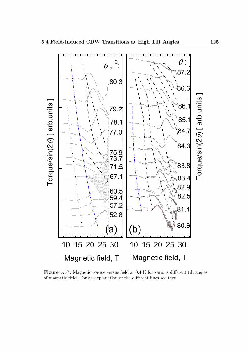
5.4 Field-Induced CDW Transitions at High Tilt Angles 125
Figure 5.57: Magnetic torque versus field at 0.4 K for various different tilt anglesof magnetic field. For an explanation of the different lines see text.
126 Results and Discussion
features in the magnetoresistance are found to correlate with those in the magnetic
torque (see e.g. Fig. 5.56), although at θ approaching 90 they become more smeared
and difficult to interpret in terms of phase transitions. The data represented by solid
lines in Fig. 5.57 have been taken at increasing B; additionally, down sweeps are
shown in the torque for 81 < θ < 84 (dashed lines) to illustrate the hysteresis.
The curves corresponding to θ < 81 have been obtained by filtering out the dHvA
oscillations from the measured signal. An example of the total signal, including the
oscillations, at θ = 67.1 is given by the grey dotted line in Fig. 5.57.
At relatively low angles, one can see a sharp kink transition which takes place at
≈ 22.5 T at 53. It gradually shifts down on tilting the field and saturates at ' 11 T
as θ approaches 90, as shown by the blue line. As Bk decreases below 20 T, the
transition becomes less pronounced, although it can still be detected up to θ ≈ 85.
Below Bk, a weak additional feature is observed up to 78 (dotted line in Fig. 5.57).
While its origin is not clear at present, it may be related to the hysteretic changes
of the magnetoresistance [109, 137] and magnetothermopower [138] observed in the
same field range earlier.
Starting from 65, new features emerge at the high-field side, moving to lower
fields with further increasing θ. Like the kink transition, they are rather sharp
and strongly hysteretic at high fields and gradually fade below 20 T. The structure
changes with increasing rate at θ → 90. At the same time the features become
less pronounced and could not be resolved above 88. While the observed behavior
is strongly suggestive of multiple phase transitions, at the moment it is difficult
to determine the exact location of each transition. However, taking into account
the character of changes in the magnetization and the hysteretic behavior, it is
reasonable, by analogy with Bk, to identify the transition points with local maxima
in the derivative (∂M/∂B)θ.
Such points are plotted in Fig. 5.59 in the form of a B − θ phase diagram. In
Fig. 5.60 the same data are replotted against 1/ cos(θ) in order to show the region
near 90 in more detail. The crosses represent Bk(θ), the empty circles correspond
to the weak feature below Bk, and the solid circles delineate the boundaries between
new subphases within the high-field CDWx state. There is a clear tendency for all
the transitions to shift to lower fields with increasing θ.
The increasingly strong angular dependence in the vicinity of θ = 90 and the
absence of the features at the exactly parallel orientation suggest that the orbital
effect, determined by the perpendicular component of magnetic field Bz = B cos(θ),
plays a crucial role. Further, since these multiple transitions happen to appear only
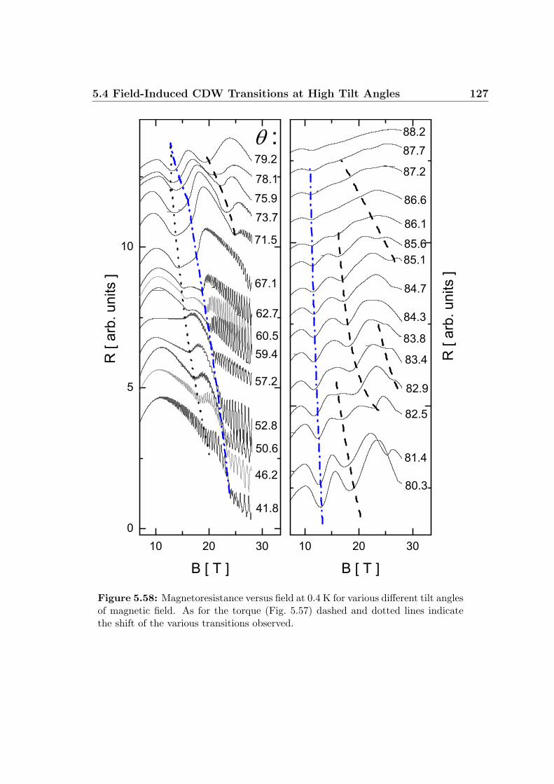
5.4 Field-Induced CDW Transitions at High Tilt Angles 127
Figure 5.58: Magnetoresistance versus field at 0.4 K for various different tilt anglesof magnetic field. As for the torque (Fig. 5.57) dashed and dotted lines indicatethe shift of the various transitions observed.
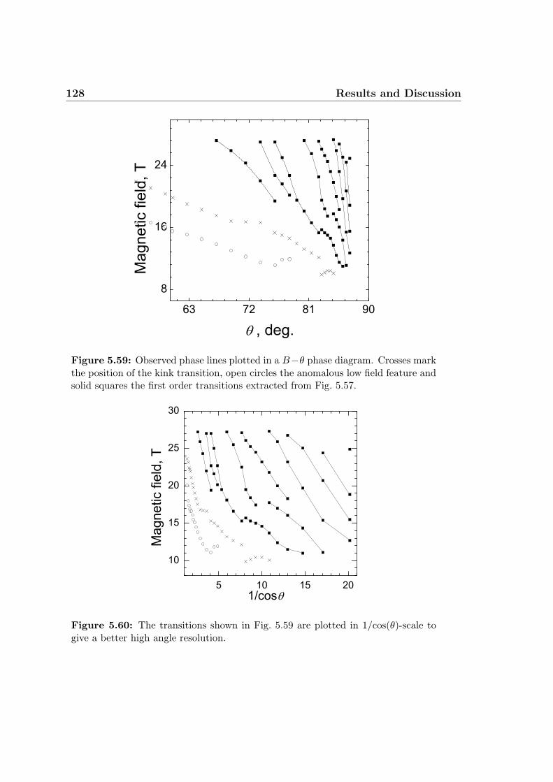
128 Results and Discussion
Figure 5.59: Observed phase lines plotted in a B−θ phase diagram. Crosses markthe position of the kink transition, open circles the anomalous low field feature andsolid squares the first order transitions extracted from Fig. 5.57.
Figure 5.60: The transitions shown in Fig. 5.59 are plotted in 1/cos(θ)-scale togive a better high angle resolution.
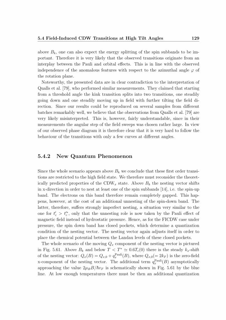
5.4 Field-Induced CDW Transitions at High Tilt Angles 129
above Bk, one can also expect the energy splitting of the spin subbands to be im-
portant. Therefore it is very likely that the observed transitions originate from an
interplay between the Pauli and orbital effects. This is in line with the observed
independence of the anomalous features with respect to the azimuthal angle ϕ of
the rotation plane.
Noteworthy, the presented data are in clear contradiction to the interpretation of
Qualls et al. [79], who performed similar measurements. They claimed that starting
from a threshold angle the kink transition splits into two transitions, one steadily
going down and one steadily moving up in field with further tilting the field di-
rection. Since our results could be reproduced on several samples from different
batches remarkably well, we believe that the observations from Qualls et al. [79] are
very likely misinterpreted. This is, however, fairly understandable, since in their
measurements the angular step of the field sweeps was chosen rather large. In view
of our observed phase diagram it is therefore clear that it is very hard to follow the
behaviour of the transitions with only a few curves at different angles.
5.4.2 New Quantum Phenomenon
Since the whole scenario appears above Bk we conclude that these first order transi-
tions are restricted to the high field state. We therefore must reconsider the theoret-
ically predicted properties of the CDWx state. Above Bk the nesting vector shifts
in x-direction in order to nest at least one of the spin subbands [14], i.e. the spin-up
band. The electrons on this band therefore remain completely gapped. This hap-
pens, however, at the cost of an additional unnesting of the spin-down band. The
latter, therefore, suffers strongly imperfect nesting, a situation very similar to the
one for t′c > t′∗c , only that the unnesting role is now taken by the Pauli effect of
magnetic field instead of hydrostatic pressure. Hence, as for the FICDW case under
pressure, the spin down band has closed pockets, which determine a quantization
condition of the nesting vector. The nesting vector again adjusts itself in order to
place the chemical potential between the Landau levels of these closed pockets.
The whole scenario of the moving Qx component of the nesting vector is pictured
in Fig. 5.61. Above Bk and below T < T ∗ ' 0.6Tc(0) there is the steady kx-shift
of the nesting vector: Qx(B) = Qx,0 + qPaulix (B), where Qx,0(= 2kF ) is the zero-field
x-component of the nesting vector. The additional term qPaulix (B) asymptotically
approaching the value 2µBB/~vF is schematically shown in Fig. 5.61 by the blue
line. At low enough temperatures there must be then an additional quantization
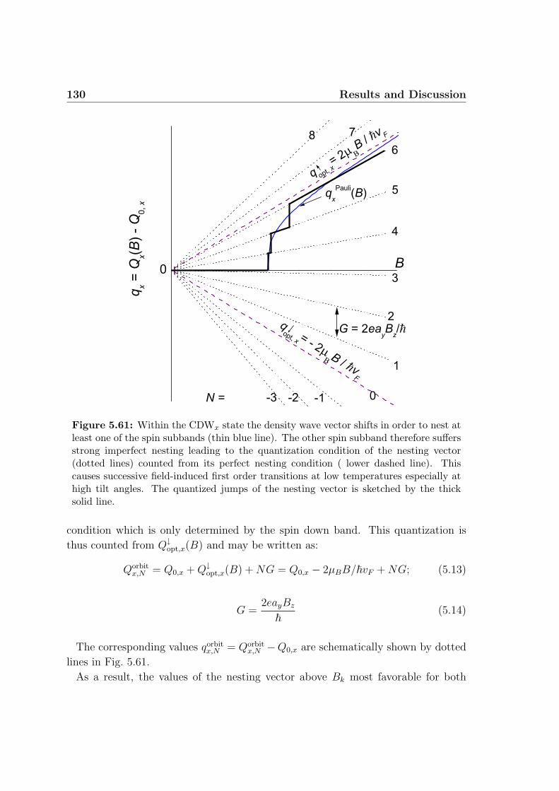
130 Results and Discussion
Figure 5.61: Within the CDWx state the density wave vector shifts in order to nest atleast one of the spin subbands (thin blue line). The other spin subband therefore suffersstrong imperfect nesting leading to the quantization condition of the nesting vector(dotted lines) counted from its perfect nesting condition ( lower dashed line). Thiscauses successive field-induced first order transitions at low temperatures especially athigh tilt angles. The quantized jumps of the nesting vector is sketched by the thicksolid line.
condition which is only determined by the spin down band. This quantization is
thus counted from Q↓opt,x(B) and may be written as:
Qorbitx,N = Q0,x + Q↓
opt,x(B) + NG = Q0,x − 2µBB/~vF + NG; (5.13)
G =2eayBz
~(5.14)
The corresponding values qorbitx,N = Qorbit
x,N −Q0,x are schematically shown by dotted
lines in Fig. 5.61.
As a result, the values of the nesting vector above Bk most favorable for both
5.4 Field-Induced CDW Transitions at High Tilt Angles 131
the spin-up and spin-down subbands should be determined by intersections of the
continuous curve qPaulix (B) with the straight lines qorbit
x,N , i.e. by the superposition of
the Pauli and quantum orbital effects. At fields close to these intersection points
we then expect the nesting vector to remain on the quantized levels. This means
that the system tries to keep both, spin up and down, type of carriers completely
gapped. Thus, with changing the field we obtain a series of first order transitions
between CDW subphases characterized by different quantized values of the nesting
vector as schematically shown by thick lines in Fig. 5.61. Remarkably, this model
implies an increase of the quantum number N with increasing B, in contrast to what
is usually observed in known orbital quantization phenomena.
Since the quantization condition is given by one spin subband while the other
one remains completely gapped, this also explains the occurrence of the first order
transitions at much higher temperatures than in the FICDW case under hydrostatic
pressure. In the latter both spin subbands contribute quantized levels. If the nesting
vector then takes a certain quantized value it may be favorable for one, but not for
the other spin band. The first order FICDW transitions are therefore predicted
only to appear at higher temperatures when both sets of quantized levels match
each other at certain ”commensurate” field directions (Eq. (5.12)).
From Fig. 5.61 it is clear that the proposed multiple transitions can only take
place if more than one quantum level intersect the qPaulix (B) curve, i.e. when
3G = 6eayBz/~ < 4µBB/~vF . (5.15)
This condition is obviously not satisfied at low θ where only one, kink transition is
observed. With increasing θ, the separation between the levels, G, proportional to
the perpendicular field component Bz decreases whereas the isotropic Pauli effect
remains unchanged. Starting from a threshold angle θ∗, the above condition becomes
fulfilled and a new transition emerges at a high field, shifting towards Bk at a further
increase of θ. In our experiment the first transition above Bk is found at θ ≈ 65.
This allows us to estimate the upper limit for the Fermi velocity in the 1D direction:
vF . 2µB/(3eay cos 65) ≈ 9× 106 cm
sec, (5.16)
which is in good agreement with the recently reported value vF = 6.5× 106 cm/sec
[136].
Thus, the proposed model explains not only the occurrence of multiple first-order
transitions above Bk, but also the threshold angle above which they start to appear
as well as the general tendency of them to shift towards Bk with further tilting the
field. Obviously, the sharpness of the transitions between the quantum orbital levels
132 Results and Discussion
should strongly depend on temperature and on the strength of the perpendicular
field component. This is consistent with the observed damping of the structure with
increasing temperature (Fig. 5.56) or at θ very close to 90 (Fig. 5.57).
There are, however, some inconsistencies between the experiment and the model
given above. The experimental phase diagram (Fig. 5.59) looks more complicated
than it would be expected within the present qualitative model: some phase lines
appear to be split, giving rise to additional subphases. This disagreement is, how-
ever, not surprising. On the one hand, we neglected the possibility of an additional
phase, CDWy (qx = 0; qy 6= 0), that may appear on tilting the magnetic field in a
certain angular and field range [14]. This has indeed been suggested by Qualls et
al. [79], but as already mentioned their determined B − θ phase diagram is very
likely incorrect. On the other hand, the orbital quantization effects may depend
on details of the anti-nesting term [139]. The latter is most likely more complex
than given by Eq. (5.6), according to band structure calculations [57,140]. This can
modify the high-field subphase structure. Further, according to newest theoretical
results from Grigoriev, under some circumstances there might exist a possibility of
two nesting vectors (one for each spin subband) spatially coexisting within the mod-
ulated CDWx(,y) state. While the physical nature of the field-induced transitions
remains the same, quantitative changes would be expected.
There are other open questions, such as the transition-like feature below Bk and
the considerable (although at a slower rate) decrease of Bk with increasing θ. Such
a strong decrease of the kink transition down to 11 T would imply a very strong
contribution from the orbital effect already at ambient pressure that can not be
expected from the phase diagram studies in section 5.1.
A development of a quantitative theory will certainly help to understand the entire
phase diagram of the present compound and to get a deeper insight into the interplay
of the Pauli and orbital effects in CDW systems.
5.4.3 Conclusion
Simultaneous measurements of the magnetic torque and magnetoresistance at dif-
ferent tilt angles of magnetic field at ambient pressure have been performed.
The already known anomalies in the magnetic torque as well as in the magnetore-
sistance occurring at ambient pressure at fields strongly inclined to the conducting
planes turn out to be a new kind of FICDW transitions. In contrast to the ones
5.4 Field-Induced CDW Transitions at High Tilt Angles 133
under hydrostatic pressure, it is now the Pauli effect of magnetic field which causes a
partial ungapping of the carriers on one of the spin-subbands. We propose a simple
model [141] in which the nesting vector within the modulated CDWx state steadily
moves in order to gap at least one of the spin-subbands, while the Landau quantiza-
tion of the partially ungapped band leads to quantized values of the nesting vector.
The superposition of both effects then determines the observed multiple phase tran-
sitions. Within this model the overall decrease of the transition fields with angle as
well as the threshold angle above which the multiple transitions start to appear, can
be understood very well.
134 Results and Discussion
5.5 Charge-Density Wave versus Superconductiv-
ity
5.5.1 Superconductivity under Hydrostatic Pressure
Within the family of organic metals α-(BEDT-TTF)2MHg(SCN)4 the compounds
with M = K, Tl, Rb have CDW ground states with slightly different transition
temperatures while the compound with M = NH4 happens to undergo a supercon-
ducting (SC) transition at ≈ 1 K [62, 63]. The absence of a density wave in the
latter salt is to the moment interpreted to be due to a higher interchain coupling
of the organic molecules within the layers [142], that strongly worsens the nesting
conditions of the open sheets of the FS. Moreover, it has been shown [143] that by
tuning the ratio of the lattice constants c/a with the aid of uniaxial strain a den-
sity wave can be even (i) induced in the NH4-compound and (ii) suppressed in the
K-compound, a SC state being stabilized at ≈ 1 K. From combined uniaxial strain
measurements and band structure calculations a major contribution to supercon-
ductivity has been proposed to come from the Q1D band [142]. As we have seen
in the previous sections a hydrostatic pressure also worsens the nesting conditions
in the K-salt, the CDW being completely suppressed in zero field at P & 2.5 kbar.
One therefore might expect a SC state also to appear under hydrostatic pressure.
Previous measurements under hydrostatic pressure by Brooks et al. [15] down to
50 mK however failed to observe any sign of superconductivity. It was only at am-
bient pressure, that the resistance decrease on lowering the temperature has been
found to significantly accelerate below 300 mK [144]. This acceleration by that time
was proposed to have a superconducting origin, due to its strong dependence on the
current level and weak magnetic field.
In order to clarify the presence of superconductivity at ambient pressure as well
as under hydrostatic pressure, detailed resistance measurements on three samples of
the M=K-compound were done down to the lowest possible temperature. For this
purpose, the Cu-Be pressure cell was mounted on a dilution refrigerator allowing
the sample to be cooled down to ≈ 20 mK. The current applied during the mea-
surement was kept ≤ 100 nA. Thus the resulting overheating of the sample during
the measurement could be estimated to be < 5 mK at 20 mK.
Surprisingly, we found superconductivity on all samples studied at such low tem-
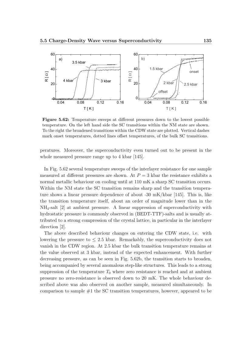
5.5 Charge-Density Wave versus Superconductivity 135
Figure 5.62: Temperature sweeps at different pressures down to the lowest possibletemperature. On the left hand side the SC transitions within the NM state are shown.To the right the broadened transitions within the CDW state are plotted. Vertical dashesmark onset temperatures, dotted lines offset temperatures, of the bulk SC transitions.
peratures. Moreover, the superconductivity even turned out to be present in the
whole measured pressure range up to 4 kbar [145].
In Fig. 5.62 several temperature sweeps of the interlayer resistance for one sample
measured at different pressures are shown. At P = 3 kbar the resistance exhibits a
normal metallic behaviour on cooling until at 110 mK a sharp SC transition occurs.
Within the NM state the SC transition remains sharp and the transition tempera-
ture shows a linear pressure dependence of about -30 mK/kbar [145]. This is, like
the transition temperature itself, about an order of magnitude lower than in the
NH4-salt [2] at ambient pressure. A linear suppression of superconductivity with
hydrostatic pressure is commonly observed in (BEDT-TTF)-salts and is usually at-
tributed to a strong compression of the crystal lattice, in particular in the interlayer
direction [2].
The above described behaviour changes on entering the CDW state, i.e. with
lowering the pressure to ≤ 2.5 kbar. Remarkably, the superconductivity does not
vanish in the CDW region. At 2.5 kbar the bulk transition temperature remains at
the value observed at 3 kbar, instead of the expected enhancement. With further
decreasing pressure, as can be seen in Fig. 5.62b, the transition starts to broaden,
being accompanied by several anomalous step-like structures. This leads to a strong
suppression of the temperature T0 where zero resistance is reached and at ambient
pressure no zero-resistance is observed down to 20 mK. The whole behaviour de-
scribed above was also observed on another sample, measured simultaneously. In
comparison to sample #1 the SC transition temperatures, however, appeared to be
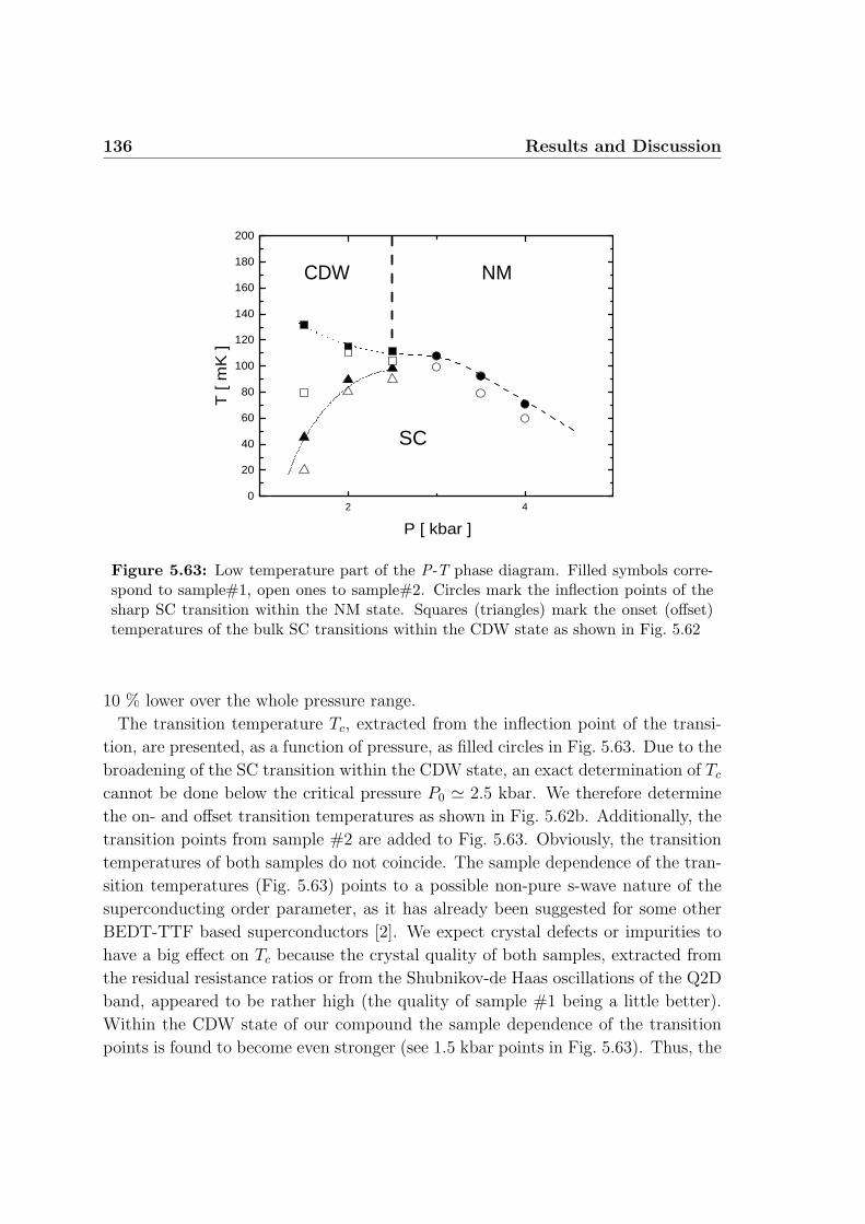
136 Results and Discussion
2 40
20
40
60
80
100
120
140
160
180
200
SC
NMCDW
T
[ mK
]
P [ kbar ]
Figure 5.63: Low temperature part of the P-T phase diagram. Filled symbols corre-spond to sample#1, open ones to sample#2. Circles mark the inflection points of thesharp SC transition within the NM state. Squares (triangles) mark the onset (offset)temperatures of the bulk SC transitions within the CDW state as shown in Fig. 5.62
10 % lower over the whole pressure range.
The transition temperature Tc, extracted from the inflection point of the transi-
tion, are presented, as a function of pressure, as filled circles in Fig. 5.63. Due to the
broadening of the SC transition within the CDW state, an exact determination of Tc
cannot be done below the critical pressure P0 ' 2.5 kbar. We therefore determine
the on- and offset transition temperatures as shown in Fig. 5.62b. Additionally, the
transition points from sample #2 are added to Fig. 5.63. Obviously, the transition
temperatures of both samples do not coincide. The sample dependence of the tran-
sition temperatures (Fig. 5.63) points to a possible non-pure s-wave nature of the
superconducting order parameter, as it has already been suggested for some other
BEDT-TTF based superconductors [2]. We expect crystal defects or impurities to
have a big effect on Tc because the crystal quality of both samples, extracted from
the residual resistance ratios or from the Shubnikov-de Haas oscillations of the Q2D
band, appeared to be rather high (the quality of sample #1 being a little better).
Within the CDW state of our compound the sample dependence of the transition
points is found to become even stronger (see 1.5 kbar points in Fig. 5.63). Thus, the
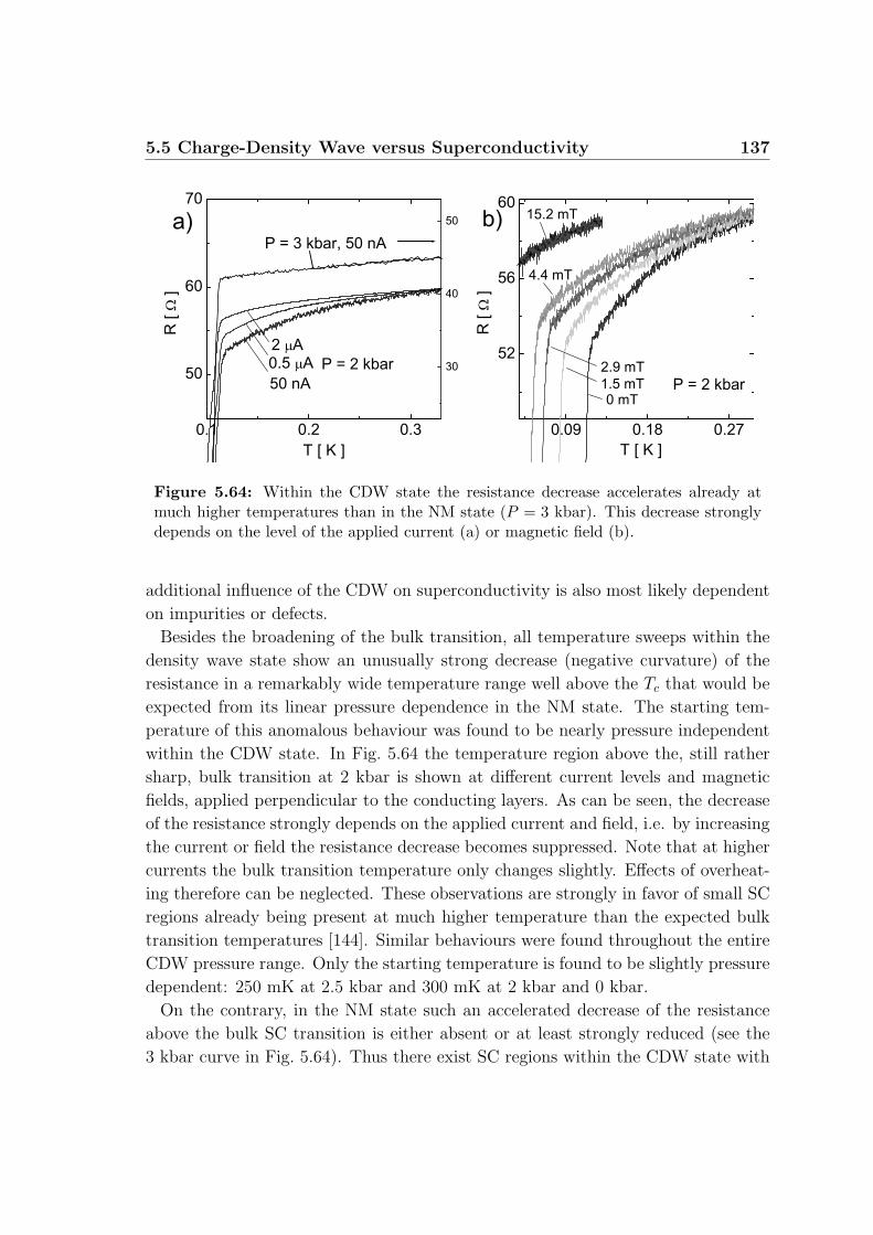
5.5 Charge-Density Wave versus Superconductivity 137
Figure 5.64: Within the CDW state the resistance decrease accelerates already atmuch higher temperatures than in the NM state (P = 3 kbar). This decrease stronglydepends on the level of the applied current (a) or magnetic field (b).
additional influence of the CDW on superconductivity is also most likely dependent
on impurities or defects.
Besides the broadening of the bulk transition, all temperature sweeps within the
density wave state show an unusually strong decrease (negative curvature) of the
resistance in a remarkably wide temperature range well above the Tc that would be
expected from its linear pressure dependence in the NM state. The starting tem-
perature of this anomalous behaviour was found to be nearly pressure independent
within the CDW state. In Fig. 5.64 the temperature region above the, still rather
sharp, bulk transition at 2 kbar is shown at different current levels and magnetic
fields, applied perpendicular to the conducting layers. As can be seen, the decrease
of the resistance strongly depends on the applied current and field, i.e. by increasing
the current or field the resistance decrease becomes suppressed. Note that at higher
currents the bulk transition temperature only changes slightly. Effects of overheat-
ing therefore can be neglected. These observations are strongly in favor of small SC
regions already being present at much higher temperature than the expected bulk
transition temperatures [144]. Similar behaviours were found throughout the entire
CDW pressure range. Only the starting temperature is found to be slightly pressure
dependent: 250 mK at 2.5 kbar and 300 mK at 2 kbar and 0 kbar.
On the contrary, in the NM state such an accelerated decrease of the resistance
above the bulk SC transition is either absent or at least strongly reduced (see the
3 kbar curve in Fig. 5.64). Thus there exist SC regions within the CDW state with
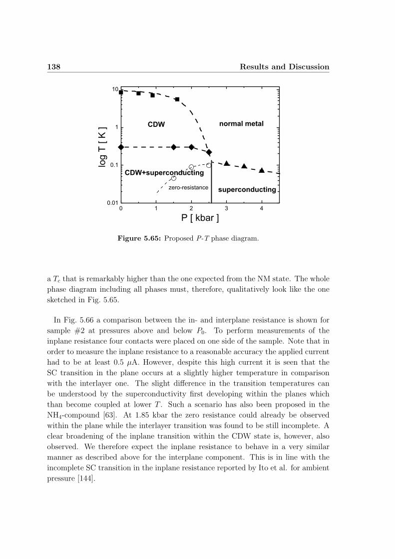
138 Results and Discussion
Figure 5.65: Proposed P-T phase diagram.
a Tc that is remarkably higher than the one expected from the NM state. The whole
phase diagram including all phases must, therefore, qualitatively look like the one
sketched in Fig. 5.65.
In Fig. 5.66 a comparison between the in- and interplane resistance is shown for
sample #2 at pressures above and below P0. To perform measurements of the
inplane resistance four contacts were placed on one side of the sample. Note that in
order to measure the inplane resistance to a reasonable accuracy the applied current
had to be at least 0.5 µA. However, despite this high current it is seen that the
SC transition in the plane occurs at a slightly higher temperature in comparison
with the interlayer one. The slight difference in the transition temperatures can
be understood by the superconductivity first developing within the planes which
than become coupled at lower T . Such a scenario has also been proposed in the
NH4-compound [63]. At 1.85 kbar the zero resistance could already be observed
within the plane while the interlayer transition was found to be still incomplete. A
clear broadening of the inplane transition within the CDW state is, however, also
observed. We therefore expect the inplane resistance to behave in a very similar
manner as described above for the interplane component. This is in line with the
incomplete SC transition in the inplane resistance reported by Ito et al. for ambient
pressure [144].
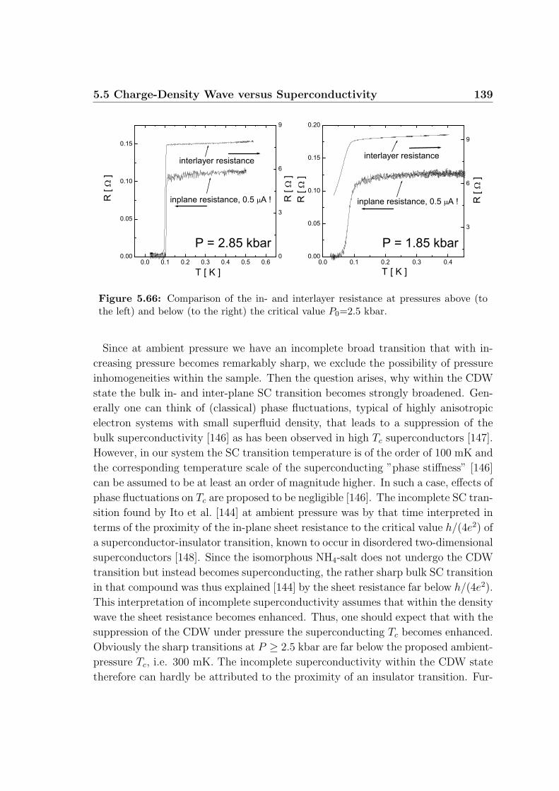
5.5 Charge-Density Wave versus Superconductivity 139
Figure 5.66: Comparison of the in- and interlayer resistance at pressures above (tothe left) and below (to the right) the critical value P0=2.5 kbar.
Since at ambient pressure we have an incomplete broad transition that with in-
creasing pressure becomes remarkably sharp, we exclude the possibility of pressure
inhomogeneities within the sample. Then the question arises, why within the CDW
state the bulk in- and inter-plane SC transition becomes strongly broadened. Gen-
erally one can think of (classical) phase fluctuations, typical of highly anisotropic
electron systems with small superfluid density, that leads to a suppression of the
bulk superconductivity [146] as has been observed in high Tc superconductors [147].
However, in our system the SC transition temperature is of the order of 100 mK and
the corresponding temperature scale of the superconducting ”phase stiffness” [146]
can be assumed to be at least an order of magnitude higher. In such a case, effects of
phase fluctuations on Tc are proposed to be negligible [146]. The incomplete SC tran-
sition found by Ito et al. [144] at ambient pressure was by that time interpreted in
terms of the proximity of the in-plane sheet resistance to the critical value h/(4e2) of
a superconductor-insulator transition, known to occur in disordered two-dimensional
superconductors [148]. Since the isomorphous NH4-salt does not undergo the CDW
transition but instead becomes superconducting, the rather sharp bulk SC transition
in that compound was thus explained [144] by the sheet resistance far below h/(4e2).
This interpretation of incomplete superconductivity assumes that within the density
wave the sheet resistance becomes enhanced. Thus, one should expect that with the
suppression of the CDW under pressure the superconducting Tc becomes enhanced.
Obviously the sharp transitions at P ≥ 2.5 kbar are far below the proposed ambient-
pressure Tc, i.e. 300 mK. The incomplete superconductivity within the CDW state
therefore can hardly be attributed to the proximity of an insulator transition. Fur-
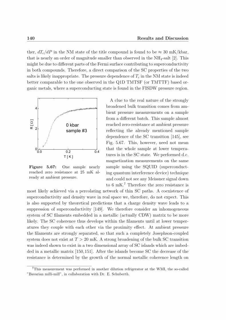
140 Results and Discussion
ther, dTc/dP in the NM state of the title compound is found to be ≈ 30 mK/kbar,
that is nearly an order of magnitude smaller than observed in the NH4-salt [2]. This
might be due to different parts of the Fermi surface contributing to superconductivity
in both compounds. Therefore, a direct comparison of the SC properties of the two
salts is likely inappropriate. The pressure dependence of Tc in the NM state is indeed
better comparable to the one observed in the Q1D TMTSF (or TMTTF) based or-
ganic metals, where a superconducting state is found in the FISDW pressure region.
Figure 5.67: One sample nearlyreached zero resistance at 25 mK al-ready at ambient pressure.
A clue to the real nature of the strongly
broadened bulk transition comes from am-
bient pressure measurements on a sample
from a different batch. This sample almost
reached zero-resistance at ambient pressure
reflecting the already mentioned sample
dependence of the SC transition [145], see
Fig. 5.67. This, however, need not mean
that the whole sample at lower tempera-
tures is in the SC state. We performed d.c.
magnetization measurements on the same
sample using the SQUID (superconduct-
ing quantum interference device) technique
and could not see any Meissner signal down
to 6 mK.7 Therefore the zero resistance is
most likely achieved via a percolating network of thin SC paths. A coexistence of
superconductivity and density wave in real space we, therefore, do not expect. This
is also supported by theoretical predictions that a charge density wave leads to a
suppression of superconductivity [149]. We therefore consider an inhomogeneous
system of SC filaments embedded in a metallic (actually CDW) matrix to be more
likely. The SC coherence thus develops within the filaments until at lower temper-
atures they couple with each other via the proximity effect. At ambient pressure
the filaments are strongly separated, so that such a completely Josephson-coupled
system does not exist at T > 20 mK. A strong broadening of the bulk SC transition
was indeed shown to exist in a two dimensional array of SC islands which are imbed-
ded in a metallic matrix [150,151]. After the islands become SC the decrease of the
resistance is determined by the growth of the normal metallic coherence length on
7This measurement was performed in another dilution refrigerator at the WMI, the so-called”Bavarian milli-mill”, in collaboration with Dr. E. Schuberth.

5.5 Charge-Density Wave versus Superconductivity 141
lowering the temperature, i.e. the proximity effect. The structures within the tran-
sitions observed in the title compound then can be explained by filaments which are
not all equidistant causing several (”bulk”-) transitions to occur. Under hydrostatic
pressure within the CDW state, we also know that small SC regions or filaments
must exist at higher temperature. Since we have no possibility at the moment to
study the magnetization under pressure, we cannot directly verify the absence of
the Meissner effect. However, as we shall see next, the filamentary nature of the
superconductivity under hydrostatic pressure is supported by measurements of the
SC transition in magnetic field.
5.5.2 Critical Magnetic Field
In Fig. 5.68 we show magnetic field sweeps, with the field directed perpendicular to
the planes, at different temperatures and two pressures above and below the critical
value P0. At zero field the bulk transition temperature at these two pressures can
be considered to be approximately the same (Fig. 5.62). At 3 kbar the transitions
remain sharp over the whole temperature range while at 2 kbar they become some-
what broadened at lower T . The critical fields Bp determined as shown in Fig. 5.68
are plotted in Fig. 5.70 for 3 different pressures. At P = 3 kbar the critical field
shows a nearly linear dependence on temperature that can be expected for coupled
SC planes in the 3D limit [147]. On entering the CDW state Bp at low temperatures
becomes dramatically enhanced, leading to a very strong positive curvature seen in
Figure 5.68: Field dependence of the interlayer resistance at various const. tempera-tures for pressures above and below P0=2.5 kbar.
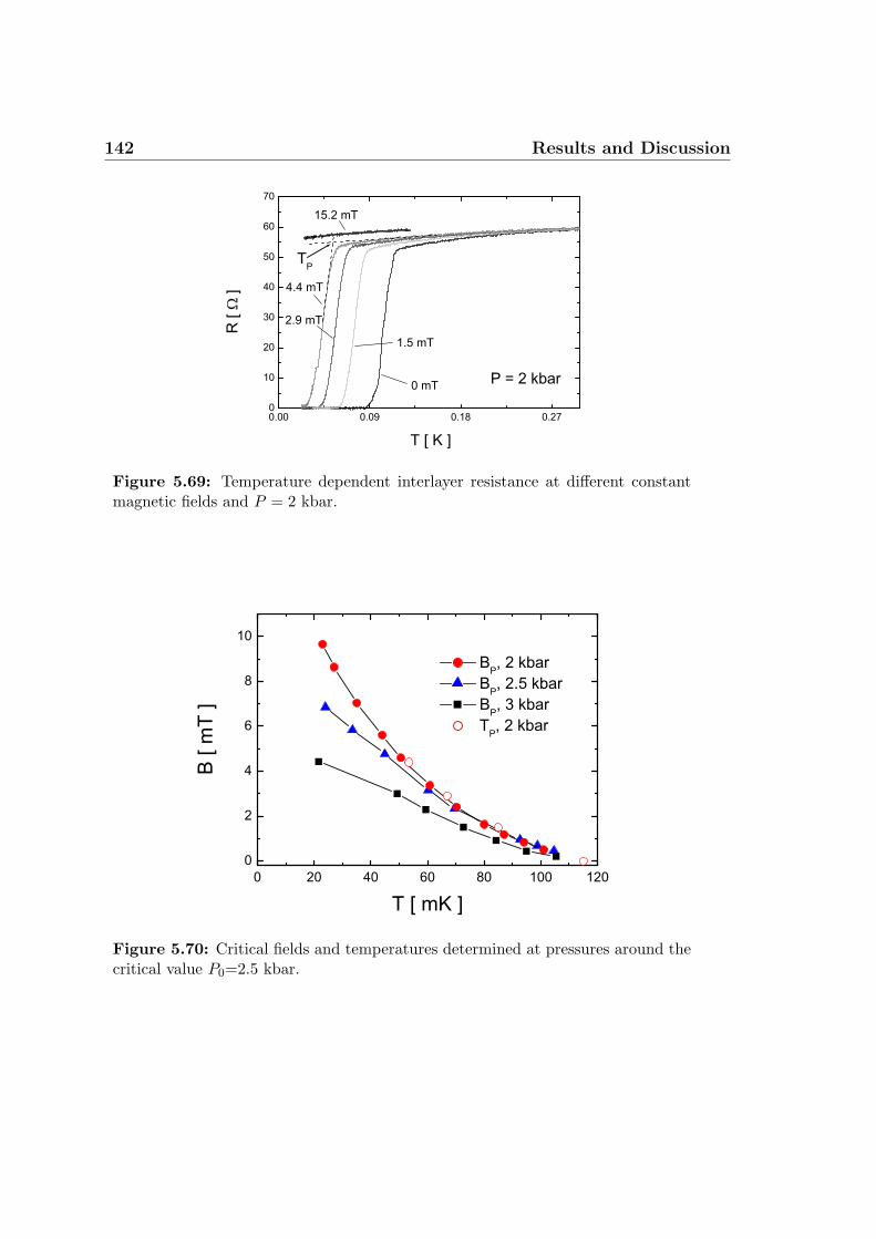
142 Results and Discussion
Figure 5.69: Temperature dependent interlayer resistance at different constantmagnetic fields and P = 2 kbar.
Figure 5.70: Critical fields and temperatures determined at pressures around thecritical value P0=2.5 kbar.
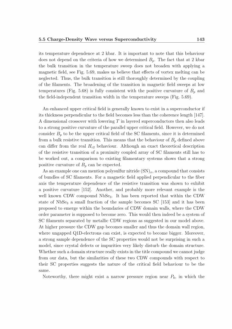
5.5 Charge-Density Wave versus Superconductivity 143
its temperature dependence at 2 kbar. It is important to note that this behaviour
does not depend on the criteria of how we determined Bp. The fact that at 2 kbar
the bulk transition in the temperature sweep does not broaden with applying a
magnetic field, see Fig. 5.69, makes us believe that effects of vortex melting can be
neglected. Thus, the bulk transition is still thoroughly determined by the coupling
of the filaments. The broadening of the transition in magnetic field sweeps at low
temperatures (Fig. 5.68) is fully consistent with the positive curvature of Bp and
the field-independent transition width in the temperature sweeps (Fig. 5.69).
An enhanced upper critical field is generally known to exist in a superconductor if
its thickness perpendicular to the field becomes less than the coherence length [147].
A dimensional crossover with lowering T in layered superconductors then also leads
to a strong positive curvature of the parallel upper critical field. However, we do not
consider Bp to be the upper critical field of the SC filaments, since it is determined
from a bulk resistive transition. This means that the behaviour of Bp defined above
can differ from the real Hc2 behaviour. Although an exact theoretical description
of the resistive transition of a proximity coupled array of SC filaments still has to
be worked out, a comparison to existing filamentary systems shows that a strong
positive curvature of Bp can be expected.
As an example one can mention polysulfur nitride (SN)x, a compound that consists
of bundles of SC filaments. For a magnetic field applied perpendicular to the fiber
axis the temperature dependence of the resistive transition was shown to exhibit
a positive curvature [152]. Another, and probably more relevant example is the
well known CDW compound NbSe3. It has been reported that within the CDW
state of NbSe3 a small fraction of the sample becomes SC [153] and it has been
proposed to emerge within the boundaries of CDW domain walls, where the CDW
order parameter is supposed to become zero. This would then indeed be a system of
SC filaments separated by metallic CDW regions as suggested in our model above.
At higher pressure the CDW gap becomes smaller and thus the domain wall region,
where ungapped Q1D-electrons can exist, is expected to become bigger. Moreover,
a strong sample dependence of the SC properties would not be surprising in such a
model, since crystal defects or impurities very likely disturb the domain structure.
Whether such a domain structure really exists in the title compound we cannot judge
from our data, but the similarities of these two CDW compounds with respect to
their SC properties suggests the nature of the critical field behaviour to be the
same.
Noteworthy, there might exist a narrow pressure region near P0, in which the
144 Results and Discussion
system becomes inhomogeneous, irrespective of any domain structure. Such an
inhomogeneous system at the phase boundary was even shown to enhance the SC
upper critical field in the spin density wave compound (TMTSF)2PF6, that would
also be expected in view of the above mentioned filamentary superconductors. This
might explain why at 2.5 kbar the transition, although still very sharp, occurs at a
lower T .
The biggest question at the moment is, why in the CDW state the superconduc-
tivity starts to appear at higher temperatures in comparison with that in the NM
state. If the superconductivity is indeed spatially restricted to the CDW domain
boundaries, one can understand, why the CDW does not completely suppress the
SC state in contradiction to what has been theoretically proposed [149]. This will,
however, not explain an enhanced SC onset temperature. In principle, in our model
above one would still expect the opposite effect, namely that the SC filament has
a reduced onset temperature due to the superconducting proximity effect. More
investigations on this topic are highly desirable.
5.5.3 Conclusion
The first direct evidence for superconductivity in α-(BEDT-TTF)2KHg(SCN)4 un-
der hydrostatic pressure is presented.
Superconductivity is found within the whole pressure range studied. Distinct dif-
ferences in the superconducting properties are observed between the CDW and the
NM state. The determined phase diagram therefore supports the above proposal of
2.5 kbar being the critical pressure P0. Within the CDW state the superconduct-
ing transitions broaden and additionally show an unusually strong decrease of the
resistance with cooling already in a higher temperature range. We associate this
finding with small superconducting filaments or regions existing in the CDW state
already at higher temperatures than expected from the NM state. This remark-
able and unexpected observation remains at present one of the biggest questions.
The broadening of the transitions as well as the finding of a pronounced positive
curvature of the critical magnetic field we explain by proximity coupled filamen-
tary superconductivity embedded in a CDW matrix. The idea of superconductivity
emerging within CDW domain boundaries is suggested.
Chapter 6
Summary
The low-temperature density-wave state existing within the organic metal α-(BEDT-
TTF)2KHg(SCN)4 below ≈ 8 K has been investigated by use of high static magnetic
fields up to 28 T and hydrostatic pressures up to 4 kbar. At ambient pressure com-
bined interlayer resistance and magnetic torque measurements have been performed,
while under pressure solely the resistance was studied.
The results presented in this thesis give further strong evidence for the already
proposed CDW nature of the low temperature state. Moreover, under certain exper-
imental conditions new kinds of CDW subphases with different density wave vectors
are most probably found to exist within different ranges of pressure and magnetic
field.
The main part of this work has been devoted to the response of a CDW system to
an applied magnetic field. Since the nesting instability arises from a very anisotropic
Q1D electron band an additional, orbital effect of the magnetic field is expected be-
sides the well-known Pauli paramagnetic one. While the former leads to an effective
one-dimensionalization of the electron motion, and consequently to a stabilization
of the density wave in magnetic field, the latter is known to suppress the CDW.
The starting point of the present investigations was the determination of the mag-
netic field-temperature (B-T ) phase diagram at different pressures with the magnetic
field directed perpendicular to the a-c planes.
Remarkably, the determined B-T phase diagrams at different pressures are found
to be extremely well described by a recent theoretical model of Zanchi et al. on the
CDW instability in Q1D electron systems at different nesting conditions. Hydro-
146 Summary
static pressure is thus found to cause a deterioration of the nesting conditions that
eventually leads to a complete suppression of the CDW at P0 ≈ 2.5 kbar at zero
magnetic field. One therefore has a perfect opportunity to determine and also tune
the nesting conditions of the present system via the applied pressure.
An important observation is, that on worsening the nesting conditions with pres-
sure the orbital effect becomes strongly enhanced and in a certain pressure and field
range exceeds the Pauli effect. This is directly reflected in an increase of the CDW
transition temperature with field.
At P > P0 we have even proven that the CDW can only exist in a magnetic field
due to the orbital effect. In this pressure region slow oscillations of the semiclassical
(background) magnetoresistance are found on sweeping the magnetic field. Several
arguments are given that these oscillations cannot be attributed to the SdH effect
but rather to the first observation of field-induced transitions between CDW sub-
phases with different nesting vectors. The latter effect can be considered as the
CDW-analogue of the well known field-induced spin density wave (FISDW) tran-
sitions observed in other organic compounds. They are theoretically expected at
P > P0 and basically arise due to the fact that part of the carriers of the quasi-one
dimensional electron system reappear as small pockets on the Fermi surface. Such
a semi-metallic electron spectrum is caused by strongly imperfect nesting.
A clear structure observed in the hysteresis between the data taken on increas-
ing and decreasing magnetic field is found to correlate with the slow background
oscillations. At certain commensurate field directions it already appears at higher
temperatures. To our opinion this gives the first solid argument for the existence of
first order transitions. The latter are indeed theoretically expected to occur due to
sudden jumps of the nesting vector between quantized values of the different CDW
subphases.
At fields strongly inclined to the conducting planes we have studied in detail the
already known anomalies in the magnetic torque as well as in the magnetoresistance
occurring at ambient pressure. These anomalies turn out to be a second kind of
field-induced CDW transitions. We propose a model, qualitatively well explaining
the data observed. Contrary to the field-induced transitions under hydrostatic pres-
sure, these new ones are now restricted to the modulated CDWx state existing at
magnetic fields above the paramagnetic limit of the low-field CDW0 state. In the
CDWx state the x-component of the nesting vector steadily increases with field in
order to completely gap one of the spin subbands. The carriers on the other sub-
147
band therefore become partially ungapped, a situation very similar to the strongly
imperfect nesting observed at P > P0. Thus, it is now the Pauli effect of magnetic
field which causes a partial ungapping of the carriers on one of the spin-subbands.
A simple model is derived including the steadily moving nesting vector and a quan-
tization condition arising due to the ungapped carriers. The superposition of both
effects then determines the observed multiple phase transitions. Within this model
the experimental observations can be qualitatively understood very well.
Besides studying the magnet field effects on the CDW state we have given the first
direct evidence for another, superconducting state under hydrostatic pressure. Sur-
prisingly, the superconductivity was found not only to exist in the pressure range,
where the CDW is already completely suppressed (at low magnetic fields), but also
within the CDW state. While above the critical pressure of 2.5 kbar there are argu-
ments for a bulk superconductivity, below 2.5 kbar there seems to be a coexistence
of the CDW and the superconducting states, which are spatially separated. The
superconductivity appears to become restricted to small superconducting regions or
filaments embedded in the CDW matrix. This would explain the absence of the
Meissner effect at ambient pressure, even when the interlayer resistance has already
vanished, as well as a strong increase of the critical magnetic field on lowering the
pressure below the critical value of 2.5 kbar. To the moment we suggest supercon-
ductivity to occur within CDW domain boundaries as has been proposed in another
CDW compound. A remarkable finding in the region of the coexisting CDW and
superconducting states is the dramatic increase of the superconducting onset tem-
perature, in comparison to that in the NM state. The reason for this unexpected
behaviour is at present not understood and needs further investigations.

148 Appendix
Appendix
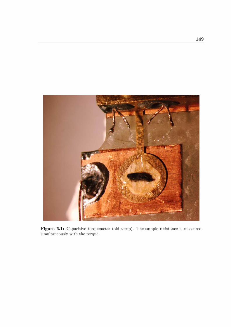
149
Figure 6.1: Capacitive torquemeter (old setup). The sample resistance is measuredsimultaneously with the torque.
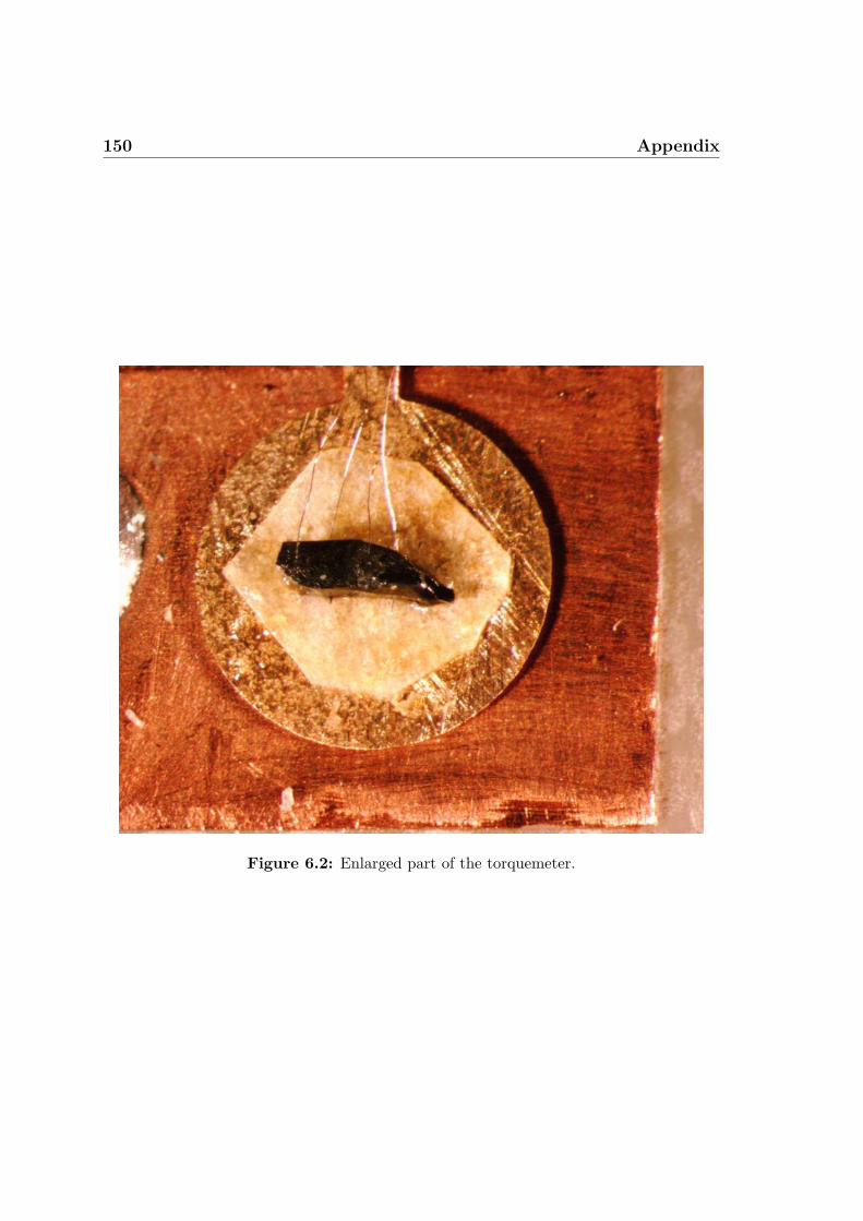
150 Appendix
Figure 6.2: Enlarged part of the torquemeter.
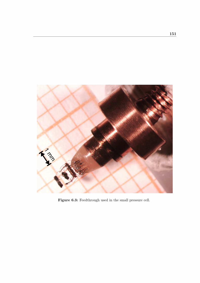
151
1m
m
Figure 6.3: Feedthrough used in the small pressure cell.
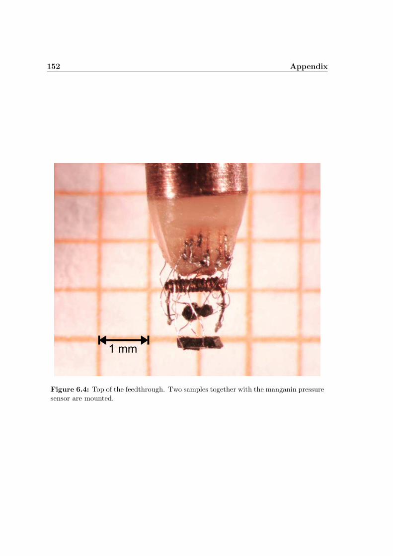
152 Appendix
1 mm
Figure 6.4: Top of the feedthrough. Two samples together with the manganin pressuresensor are mounted.
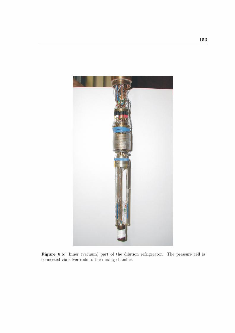
153
Figure 6.5: Inner (vacuum) part of the dilution refrigerator. The pressure cell isconnected via silver rods to the mixing chamber.

154 Bibliography
Bibliography
[1] W. A. Little. Phys. Rev., 134:A1416, 1964.
[2] T. Ishiguro, K. Yamaji, and G.Saito. Organic Superconductors, 2nd edition.
Springer-Verlag Berlin Heidelberg, 1998.
[3] D. Jerome. Science, 252:1509, 1991.
[4] D. Jerome. Solid State Commun., 92:89, 1994.
[5] P. M. Chaikin. J. Phys. I France, 6:1875, 1996.
[6] S. Uji, H. Shinagawa, T. Terashima, T. Yakabe, Y. Terai, M. Tokumoto,
A. Kobayashi, H. Tanaka, and H. Kobayashi. Nature, 410:908, 2001.
[7] S. Uji, T. Terashima, C. Terakura, T. Yakabe, Y. Terai, S. Yasuzuka,
Y. Ymanaka, M. Tokumoto, A. Kobayashi, F. Sakai, H. Tanaka, H. Kobayashi,
L. Balicas, and J. S. Brooks. J. Phys. Soc. Jpn., 72:369, 2003.
[8] J. Wosnitza. Studies of High-Temperature Superconductivity, 34:97, 2000.
edited by A. Narlikar (Nova Science Publishers, Huntington).
[9] J. Wosnitza. Fermi Surfaces of Low-Dimensional Organic Metals and Super-
conductors. Springer-Verlag Berlin Heidelberg, 1996.
[10] T. Osada, R. Yagi, A. Kawasumi, S. Kagoshima, N. Miura, M. Oshima, and
G. Saito. Phys. Rev. B, 41:5428(R), 1990.
[11] M. V. Kartsovnik, A. E. Kovalev, and N. D. Kushch. J. Phys. I France, 3:1187,
1993.
[12] P. Christ, W. Biberacher, M. V. Kartsovnik, E. Steep, E. Balthes, H. Weiss,
and H. Muller. JETP Lett., 71:303, 2000.
156 Bibliography
[13] R. H. McKenzie. cond-mat/9706235, unpublished, 1997.
[14] D. Zanchi, A. Bjelis, and G. Montambaux. Phys. Rev. B, 53:1240, 1996.
[15] J. Brooks, K. Chen, S. Klepper, S. Valfells, G. Athas, Y. Tanaka, T. Kinoshita,
M. Tokomoto, H. Anzai, and C. Agosta. Phys. Rev. B, 52:14457, 1995.
[16] N. Hanasaki, S. Kagoshima, N. Miura, and G. Saito. J. Phys. Soc. Jap.,
65:1010, 1996.
[17] J. Lindhard. K. Dan. Vidensk. Selsk. Mat.-Fys. Medd., 28:8, 1954.
[18] J. M. Ziman. Principles of the Theory of Solids. Cambridge University Press,
1964.
[19] G. Gruner. Density Waves in Solids. Addison Wesley, 1994.
[20] S. Kagoshima, H. Nagasawa, and T. Sambongi. Physics in One Dimension.
Springer Series in Solid-State Science 72, Springer Verlag Berlin Heidelberg
New York Paris Tokyo, 1988.
[21] D. Jerome and H. J. Schulz. Advances in Physics, 31(4):299, 1982.
[22] L. P. Gorkov and A. G. Lebed. J. Phys. (Paris) Lett., 45:L433, 1984.
[23] J. Solynom. Adv. Phys., 28:201, 1979.
[24] T. M. Rice. Physics in One Dimension. eds. J. Bernasconi and T. Schneider,
Springer-Verlag, 1981.
[25] S. Brown and G. Gruner. Spektrum der Wissenschaft, page 64, June 1994.
[26] W. Dieterich and P. Fulde. Z. Physik, 265:239, 1973.
[27] G. Sarma. J. Phys. Chem. Solids, 24:1029, 1963.
[28] A. I. Buzdin and V. V. Tugushev. JETP, 58:428, 1983.
[29] A. Bjelis, D. Zanchi, and G. Montambaux. J. Phys. IV France, 9:PR10–203,
1999.
[30] G. Montambaux. Phys. Rev. B, 38:4788, 1988.
[31] J. F. Kwak, J. E. Schirber, P. M. Chaikin, J. M. Williams, H.-H. Wang, and
L. Y. Chiang. Phys. Rev. Lett., 56:972, 1986.
157
[32] G. M. Danner, P. M. Chaikin, and S. T. Hannahs. Phys. Rev. B, 53:2727,
1996.
[33] W. Kang, S. T. Hannahs, and P. M. Chaikin. Phys. Rev. Lett., 70:3091, 1993.
[34] V. M. Yakovenko. Europhys. Lett., 3:1041, 1987.
[35] D. Schoenberg. Magnetic oscillations in metals. Cambridge University Press,
1984.
[36] L. Onsager. Phil. Mag., 43:1006, 1952.
[37] W. J. de Haas and P. M. van Alphen. Proc. Netherlands Roy. Acad. Sci.,
33:1106, 1930.
[38] R. B. Dingle. Proc. Roy. Soc., 211:517, 1952.
[39] L. W. Shubnikov and W. J. de Haas. Proc. Netherlands Roy. Acad. Sci.,
33:p.130 and 163, 1930.
[40] E. N. Adams and T. D. Holstein. J. Phys. Chem. Solids, 10:254, 1959.
[41] A. A. Abrikosov. Fundamentals of the Theory of Metals. Elsevier Sciense
Publishers B.V., 1988.
[42] N. Harisson, R. Bogaerts, P. H. P. Reinders, J. Singleton, S. J. Blundell, and
F. Herlach. Phys. Rev. B, 54:9977, 1996.
[43] M. A. Itskovsky and T. Maniv. Phys. Rev. B, 64:174421, 2001.
[44] M. V. Kartsovnik. Chem. Rev., 104:5737, 2004.
[45] E. I. Blount. Phys. Rev. Lett., 126:1636, 1962.
[46] T. Osada, S. Kagoshima, and N. Miura. Phys. Rev. B, 46:1812, 1992.
[47] M. J. Naughton, O. H. Chung, L. Y. Chiang, and J. S. Brooks. Mater. Res.
Soc. Symp. Proc., 173:257, 1990.
[48] T. Osada, A. Kawasumi, S. Kagoshima, N. Miura, and G. Saito. Phys. Rev.
Lett., 66:1525, 1991.
[49] T. Osada, A. Kawasumi, S. Kagoshima, N. Miura, and G. Saito. Physica C,
185-189:2697, 1991.
158 Bibliography
[50] M. J. Naughton, O. H. Chung, M. Chaparala, X. Bu, and P. Coppens. Phys.
Rev. Lett., 67:3712, 1991.
[51] K. Yamaji. J. Phys. Soc. Jpn., 58:1520, 1989.
[52] R. Yagi, Y. Iye, T. Osada, and S. Kagoshima. J. Phys. Soc. Jpn., 59:3069,
1990.
[53] V.G. Peschansky, J.A. Lopes, and T.G. Yao. J. Phys. I France, 1:1469, 1991.
[54] M. V. Kartsovnik, V. N. Laukhin, S. I. Pesotskii, I. F. Schegolev, and V. M.
Yakovenko. J. Phys. I France, 2:89, 1992.
[55] Y. Kurihara. J. Phys. Soc. Jpn., 61:975, 1992.
[56] A. B. Pippard. Magnetoresistance in Metals. Cambridge University Press,
1989.
[57] R. Rousseau, M.-L. Doublet, E. Canadell, R. P. Shibaeva, S. S. Khasanov,
L. P. Rozenberg, N. D. Kushch, and E. B. Yagubskii. J. Phys. I France,
6:1527, 1996.
[58] P. C. W. Leung, T. J. Emge, M. A. Beno, H. H. Wang, J. M. Williams,
V. Petricek, and P. Coppens. J. Am. Chem. Soc., 107:6184, 1985.
[59] H. Mori, S. Tanaka, M. Oshima, G. Saito, T. Mori, Y. Murayama, and
H. Iinokuchi. Bull. Chem. Soc. Jpn., 63:2183, 1991.
[60] H. Sato, H. Taniguchi, Y. Nakazawa, A. Kawamoto, K. Kato, and K. Kanoda.
Synth. Met., 70:915, 1995.
[61] J. Singleton. Rep. Prog. Phys., 63:1111, 2000.
[62] H. H. Wang, K. D. Carson, U. Geiser, W. K. Kwok, M. D. Vashon, J. E.
Thompson, N. F. Larsen, G. D. Mccabe, R. S. Hulscher, and J. M. Williams.
Physica C, 166:57, 1990.
[63] H. Taniguchi, H. Sato, Y. Nakazawa, and K. Kanoda. Phys. Rev. B,
53:8879(R), 1996.
[64] A. E. Kovalev, M. V. Kartsovnik, R. P. Shibaeva, L. P. Rozenberg, and I. F.
Schegolev. Solid State Commun., 89:575, 1994.
159
[65] J. S. Boebinger, G. Montambaux, M. L. Kaplan, R. C. Haddon, S. V. Chich-
ester, and L. Y. Chiang. Phys. Rev. Lett., 64:591, 1990.
[66] M. V. Kartsovnik and V. N. Laukhin. J. Phys. I France, 6:1753, 1996.
[67] Y. Iye, R. Yagi, N. Hanasaki, S. Kagoshima, H. Mori, H. Fujimoto, and
G. Saito. J. Phys. Soc. Jpn., 63:674, 1994.
[68] T. Sasaki and N. Toyota. Phys. Rev. B, 49:10120, 1994.
[69] T. Sasaki, H. Sato, and N. Toyota. Synth. Met., 41-43:2211, 1991.
[70] F. L. Pratt, T. Sasaki, and N. Toyota. Phys. Rev. Lett., 74:3892, 1995.
[71] R. Tsuchiya, T. Nakamura, T. Takahashi, T. Sasaki, and N. Toyota. Synth.
Met., 70:965, 1995.
[72] T. Miyagawa, A. Kawamoto, and K. Kanoda. Phys. Rev. B., 56:8487(R), 1997.
[73] P. Christ, W. Biberacher, H. Muller, K. Andres, E. Steep, and A. G. M.
Jansen. Synth. Metals, 70:823, 1996.
[74] P. Christ. Dissertation an der Fakultat fur Physik an der Technischen Univr-
sitat Munchen. 1998.
[75] A. Kovalev and H. Muller. Synth.Metals, 86, 1997.
[76] T. Sasaki, A. Lebed, and T. Fukase. Phys. Rev. B, 54:12969, 1996.
[77] M. V. Kartsovnik, W. Biberacher, E. Steep, P. Christ, K. Andres, A. G. M.
Jansen, and H. Muller. Synth. Metals, 86:1933, 1997.
[78] N. Harrison, L. Balicas, J. S. Brooks, and M. Tokumoto. Phys. Rev. B,
62:14212, 2000.
[79] J. S. Qualls, L. Balicas, J. S. Brooks, N. Harrison, L. K. Montgomery, and
M. Tokumoto. Phys. Rev. B, 62:10008, 2000.
[80] P. Fulde and R. A. Ferrell. Phys. Rev., 135:A550, 1964.
[81] A. I. Larkin and Y. N. Ovchinikov. Sov. Phys. JETP, 20:762, 1965.
[82] M. Basletic, B. Korin-Hamzic, M. V. Kartsovnik, and H. Muller. Synth. Met.,
120:1021, 2001.
160 Bibliography
[83] P. Foury-Leylekian, S. Ravy, J. P. Pouget, and Muller. Synth. Met., 137:1271,
2003.
[84] A. House, S. Blundell, M. M. Honold, J. Singleton, J. A. A. J. Perenboom,
W. Hayes, M. Kurmoo, and P. Day. J. Phys. Cond. Mat., 8:8829, 1996.
[85] R. H. McKenzie, G. J. Athas, J. S. Brooks, R. G. Clark, A. S. Dzurak,
R. Newbury, R. P. Starrett, A. Skougarevsky, M. Tokumoto, N. Kinoshita,
T. Kinoshita, and Y. Tanaka. Phys. Rev. B, 54:8289(R), 1996.
[86] L. I. Buravov, N. D. Kushch, V. N. Laukhin, A. G. Khomenko, E. B. Yagubskii,
M. V. Kartsovnik, A. E. Kovalev, L. P. Rozenberg, R. P. Shibaeva, M. A.
Tanatar, V. S. Yefanof, V. V. Dyakin, and V. A. Bondarenko. J. Phys. I
France, 4:441, 1994.
[87] P. Christ, W. Biberacher, H. Muller, and K. Andres. Solid State Commun.,
91:451, 1994.
[88] I. L. Spain and S. Segall. Cryogenics, 11:26, 1971.
[89] L. C. Towle. Appl. Phys. Lett., 10:317, 1967.
[90] S. Yamamoto. Bull. of the N.R.L.M., 24:25, 1972.
[91] H. Fujiwara, H. Kadomatsu, K. Thoma, and Rev. Sci. Instrum. Rev. Sci.
Instrum., 51:1345, 1980.
[92] D. Andres. Diploma thesis, TU Munchen, 2000.
[93] M. V. Kartsovnik, D. Andres, W. Biberacher, P. Christ, E. Steep, E. Balthes,
H. Weiss, H. Muller, and N. D. Kushch. Synth. Metals, 120:687, 2001.
[94] A. Schegolev, V. Laukhin, A. Khomenko, M. Kartsovnik, R. Shibaeva,
L. Rozenberg, and A. Kovalev. J. Phys. I France, 2:2123, 1992.
[95] Y. Hasegawa and H. Fukuyama. J. Phys. Soc. Jpn., 55:3978, 1986.
[96] K. Yamaji. J. Phys. Soc. Jpn., 51:2787, 1982.
[97] N. Biskup, S. Tomic, and D. Jerome. Phys. Rev. B, 51:17972, 1995.
[98] N. Biskup, J. A. A. J. Perenboom, J. S. Qualls, and J. S. Brooks. Solid State
Commun., 107:503, 1998.
161
[99] B. Hamzic, G. Creuzet, and C. Lenoir. J. Phys. F: Met.Phys., 17:2267, 1987.
[100] L. Forro, K. Biljakovic, J. R. Cooper, and K. Bechgaard. Phys. Rev. B,
29:2839, 1984.
[101] R. H. McKenzie, J. S. Qualls, S. Y. Han, and J. S. Brooks. Phys. Rev. B,
57:11854, 1998.
[102] R. V. Coleman, M. P. Everson, Hao-An Lu, , A. Johnson, and L. M. Falicov.
Phys. Rev. B, 41:460, 1990.
[103] D. Andres, M. V. Kartsovnik, W. Biberacher, H. Weiss, E. Balthes, H. Muller,
and N. Kushch. Phys. Rev. B, 64:161104(R), 2001.
[104] R. W. Stark and C. B. Friedberg. Phys. Rev. Lett., 26:556, 1971.
[105] S. Uji, H. Aoki, J. S. Brooks, A. S. Perel, G. J. Athas, S. J. Klepper, C. C.
Agosta, D. A. Howe, M. Tokumoto, N. Kinoshita, Y. Tanaka, and H. Anzai.
Solid State Commun., 88:683, 1993.
[106] A. House, C. J. Hawoth, J. M. Caulfield, S. Blundell, M. M. Honold, J. Sin-
gleton, W. Hayes, S. M. Hayden, P. Meeson, M. Springford, M. Kurmoo, and
P. Day. J. Phys. Cond. Mat., 8:10361, 1996.
[107] N. Harrison, N. Biskup, J. S. Brooks, L. Balicas, and M. Tokumoto. Phys.
Rev. B, 63:195102, 2001.
[108] G. J. Athas, J. S. Brooks, S. Valfells, S. J. Klepper, M. Tokumoto, N. Ki-
noshita, T. Kinoshita, and Y. Tanaka. Phys. Rev. B, 34:863, 1994.
[109] N. Harrison. Phys. Rev. Lett., 83:1395, 1999.
[110] P. Monceau. Solid State Commun., 24:331, 1977.
[111] C. E. Campos, P. S. Sandhu, J. S. Brooks, and T. Ziman. Phys. Rev. B,
53:12725, 1996.
[112] M. M. Honold, N. Harrison, J. Singleton, M.-S. Nam, S. J. Blundell, C. H.
Mielke, M.V. Kartsovnik, and N.D. Kushch. Phys. Rev. B, 59:10417(R), 1999.
[113] T. Sasaki and N. Toyota. Phys. Rev. B, 48:11457(R), 1993.
[114] E. M. Lifshitz and A. M. Kosevich. J. Phys. Chem. Solids, 4:1, 1956.
162 Bibliography
[115] N. Harrison, C. H. Mielke, J. Singleton, J. S. Brooks, and M. Tokumoto. J.
Phys.: Condens. Matter, 13:L389–L395, 2001.
[116] S. Hill, P.S. Sandhu, J.S. Qualls, J.S. Brooks, M. Tokumoto, N. Kinoshita,
T. Kinoshita, and Y. Tanaka. Phys. Rev. B, 55:4891(R), 1997.
[117] M. M. Honold, N. Harrison, J. Singleton, H. Yaguchi, C. H. Mielke, D. Rickel,
I. Deckers, P. H. P. Reinders, F. Herlach, M. Kurmoo, and P. Day. J. Phys.:
Condens. Matter, 9:L533, 1997.
[118] N. Harrison. Phys. Rev. R, 66:121101(R), 2002.
[119] N. Harrison, J. Singleton, A. Bangura, A. Ardavan, P. A. Goddard, R. D.
McDonald, and L. K. Montgomery. Phys. Rev. B, 69:165103, 2004.
[120] S. Uji, J.S. Brooks, M. Chaparala, L. Seger, T. Szabo, M. Tokumoto, N. Ki-
noshita, T. Kinoshita, Y. Tanaka, and H. Anzai. Solid State Commun.,
100:825, 1996.
[121] N. Harrison, A. House, I.Deckers, J. Caulfield, J. Singleton, F. Herlach,
W. Hayes, M. Kurmoo, and P. Day. Phys. Rev. B, 52:5584, 1996.
[122] A. House, W. Lubczynski, S. Blundell, J. Singleton, W. Hayes, M. Kurmoo,
and P. Day. J. Phys. Cond. Mat., 8:10377, 1996.
[123] T. Sasaki and T. Fukase. Phys. Rev. B, 59:13872, 1999.
[124] S. Kawamata, K. Okuda, I. Kakeyab, K. Kindo, T. Sasaki, and N. Toyotad.
Synth. Metals, 86:2015, 1997.
[125] K. Yamaji. J. Phys. Soc. Jpn., 53:2189, 1984.
[126] G. Montambaux, M. Heritier, and P. Lederer. Phys. Rev. Lett., 55:2078, 1985.
[127] A. G. Lebed. Pis’ma Zh. Eksp. Teor. Fiz., 43:137, 1986.
[128] K. Yamaji. J. Phys. Soc. Jpn., 56:1841, 1987.
[129] A. G. Lebed. Pis’ma Zh. Eksp. Teor. Fiz., 78:170, 2003.
[130] K. Yamaji. Synth. Met., 13:29, 1986.
[131] A. G. Lebed. Pis’ma Zh. Eksp. Teor. Fiz., 72:205, 2000.
163
[132] A. G. Lebed. Phys. Rev. Lett., 88:177001, 2002.
[133] K. Sengupta and N. Dupuis. cond-mat/0302142, unpublished, 2003.
[134] A. V. Kornilov, V. M. Pudalov, Y. Kitaoka, K. Ishida, T. Mito, J. S. Brooks,
J. S. Qualls, J. A. A. J. Perenboom, N. Tateiwa, and T. C. Kobayashi. Phys.
Rev. B, 65:060404(R), 2002.
[135] W. Kang. Thesis, Princeton University. 1993.
[136] A. E. Kovalev, S. Hill, and J. S. Qualls. Phys. Rev. B, 66:134513, 2002.
[137] C. Proust, A. Audouard, A. Kovalev, D. Vignolles, M. Kartsovnik,
L. Brossard, and N. Kushch. Phys. Rev. B, 62:2388, 2000.
[138] E. S. Choi, J. S. Brooks, and J. S. Qualls. Phys. Rev. B, 65:205119, 2002.
[139] D. Zanchi and G. Montambaux. Phys. Rev. Lett., 77:366, 1996.
[140] M. Gusmao and T. Ziman. Phys. Rev. B, 54:16663, 1996.
[141] D. Andres, M. Kartsovnik, P. D. Grigoriev, W. Biberacher, and H. Muller.
Phys. Rev. B, 68:201101(R), 2003.
[142] R. Kondo, S. Kagoshima, and M. Maesato. Phys. Rev. B, 67:134519, 2003.
[143] M. Maesato, Y. Kaga, R. Kondo, and S. Kagoshima. Phys. Rev. B., 64:155104,
2001.
[144] H. Ito, M. V. Kartsovnik, H. Ishimoto, K. Kono, H. Mori, N. D. Kushch,
G. Saito, T. Ishiguro, and S. Tanaka. Synth. Met., 70:899, 1995.
[145] D. Andres, M. V. Kartsovnik, W. Biberacher, K. Neumaier, and H. Muller. J.
Phys. IV France, 12:PR9–87, 2002.
[146] V. J. Emery and S. A. Kivelson. Nature, 374:434, 1995.
[147] M. Tinkham. Introduction to Superconductivity. McGraw-Hill International
editions, 1996.
[148] M. Fisher. Phys. Rev. Lett., 65:923, 1990.
[149] A. M. Gabovich, A. I. Voitenko, and M. Ausloos. Phys. Rep., 367:583, 2002.
164 Bibliography
[150] D. J. Resnick, J. C. Garland, J. T. Boyd, S. Shoemaker, and R. S. Newrock.
Phys. Rev. Lett., 47:1542, 1981.
[151] D. W. Abraham, C. J. Lobb, M. Tinkham, and T. M. Klapwijk. Phys. Rev.
B, 26:5268, 1982.
[152] L. J. Azevedo, W. G. Clark, G. Deutscher, R. L. Greene, G. B. Street, and
L. J. Suter. Solid State Commun., 19:197, 1976.
[153] A. Briggs, P. Monceau, M. Nunez-Regueiro, M. Ribault, and J. Richard. J.
Phys., 42:1453, 1981.
Publication List 165
Publication List
D. Andres, M. V. Kartsovnik, W. Biberacher, H. Weiss, E. Balthes, H. Muller, and
N. Kushch.
Phys. Rev. B, 64:161104(R), 2001.
D. Andres, M. Kartsovnik, P. D. Grigoriev, W. Biberacher, and H. Muller.
Phys. Rev. B, 68:201101(R), 2003.
D. Andres, M. V. Kartsovnik, W. Biberacher, K. Neumaier, and H. Muller.
J. Phys. IV France, 12:PR9–87, 2002.
D. Andres, M. V. Kartsovnik, W. Biberacher, T. Togonidze, H. Weiss, E. Balthes,
and N. Kushch.
Synth. Met., 120:841, 2001.
M. V. Kartsovnik, D. Andres, W. Biberacher, P. Christ, E. Steep, E. Balthes,
H. Weiss, H. Muller, and N. D. Kushch.
Synth. Met., 120:687, 2001.
M. V. Kartsovnik, D. Andres, W. Biberacher, P. D. Grigoriev, E. A. Schuberth, and
H. Muller.
J. Phys. IV France, 114:191, 2004.
M. V. Kartsovnik, D. Andres, P. D. Grigoriev, W. Biberacher, and H. Muller.
Physica B: Condensed Matter, 346-347:368, 2004.
A.E. Kovalev, M.V. Kartsovnik, D. Andres, A.G.M. Jansen, and N.D. Kushch.
Synth. Met., 133-134:131, 2003.
P. Christ, W. Biberacher, D. Andres, M. V. Kartsovnik, E. Balthes, H. Weiss, and
H. Muller.
Synth. Met., 120:1019, 2001.
W. Biberacher, P. Christ, M. V. Kartsovnik, D. Andres, and H. Muller.
J. Phys. IV France, 114:291, 2004.

166
Acknowledgements 167
AcknowledgementsOf course, this work could not have been done without the help of many people to
whom I would like to express my gratitude. In particular, I would like to thank...
• our organic metal team,
– Mark Kartsovnik, my academic advisor, for teaching me all the exper-
imental and physical know-how, without exception taking his time for
answering and discussing my questions and always motivating me for
new interesting tasks.
– Werner Biberacher, for all his contribution to this work, and especially
for his expertize in the magnetic torque experiments.
• Prof. Rudolf Gross, for accepting me as a PhD student.
• Pavel Grigoriev, a young theorist, always full of energy, for his theoretical ideas
and for the fruitful discussions.
• Karl Neumaier, for the experimental support on the dilution refrigerator and
for teaching me some experimental low temperature physics.
• Harald Muller and Natasha Kushch, for the synthesis of many high quality
samples.
• the WMI workshop, in particular Helmut Thies, for doing an outstanding job
on fabricating the new designed 2-axes rotator.
• the staff at the high field lab in Grenoble, for their experimental support.
• Joachim Geismann, for the technical expert advice on the Helium-pressure
station.
• Sergei Pesotskii, for his experimental contribution.
• Erwin Schuberth, for the joint SQUID measurement in the ”milli-mill”.
• Wolfgang Schmitt, for the photographic equipment.
• all the people at the WMI, for their readiness to help and for creating a nice
working atmosphere.
• my family