Effects of High Magnetic Fields and Hydrostatic Pressure on ...
Mixed Models for Longitudinal Ordinal and NominalData
Hedeker, D. (2008). Multilevel models for ordinal and nominal variables. In J.de Leeuw & E. Meijer (Eds.), Handbook of Multilevel Analysis. Springer, NewYork.
Hedeker, D. (2005). Generalized linear mixed models. In B. Everitt & D.Howell (Eds.), Encyclopedia of Statistics in Behavioral Science. Wiley.
Chapters 10 & 11 in Hedeker, D. & Gibbons, R.D. (2006). Longitudinal DataAnalysis. Wiley.
1
Why analyze as ordinal?
• Efficiency: Armstrong & Sloan (1989, Amer Jrn of Epid)report efficiency losses between 89% to 99% comparing anordinal to continuous outcome, depending on the number ofcategories and distribution within the ordinal categories.
• Bias: continuous model can yield correlated residuals andregressors when applied to ordinal outcomes, because thecontinuous model does not take into account the ceiling andfloor effects of the ordinal outcome. This can result in biasedestimates of regression coefficients and is most critical whenthe ordinal variables is highly skewed.
• Logic: continuous model can yield predicted values outside ofthe range of the ordinal variable.
2

Proportional Odds Model - McCullagh (1980)
log
P (Y ≤ c)
1 − P (Y ≤ c)
= γc − x′β
c = 1, . . . , C − 1 for the C categories of the ordinal outcome
x = vector of explanatory variables (plus the intercept)
γc = thresholds; reflect cumulative odds when x = 0 (for identification: γ1 = 0 or β0 = 0)
• positive association between x and Y is reflected by β > 0
• the effect of x is assumed to be the same for each cumulativeodds ratio
• odds that the response is greater than or equal to c (for fixedc) is multiplied by eβ for every unit change in x:
1 − P (Y ≤ c)
P (Y ≤ c)
= e−γc × (eβ)x
3

Ordinal Model for Dichotomous Response: same as itever was!
log
P (Y = 0)
1 − P (Y = 0)
= 0 − x′β
P (Y = 0)
1 − P (Y = 0)= exp(0 − x′β)
1 − P (Y = 0)
P (Y = 0)= [exp(0 − x′β)]
−1
1 − P (Y = 0)
P (Y = 0)= exp(x′β)
log
P (Y = 1)
1 − P (Y = 1)
= x′β
4
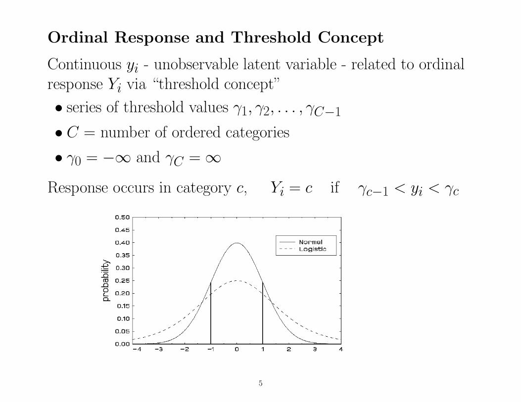
Ordinal Response and Threshold Concept
Continuous yi - unobservable latent variable - related to ordinalresponse Yi via “threshold concept”
• series of threshold values γ1, γ2, . . . , γC−1
• C = number of ordered categories
• γ0 = −∞ and γC = ∞
Response occurs in category c, Yi = c if γc−1 < yi < γc
5

The Threshold Concept in Practice
“How was your day?”(what is your level of satisfaction today?)
• Satisfaction may be continuous, but we sometimes emit anordinal response:
6
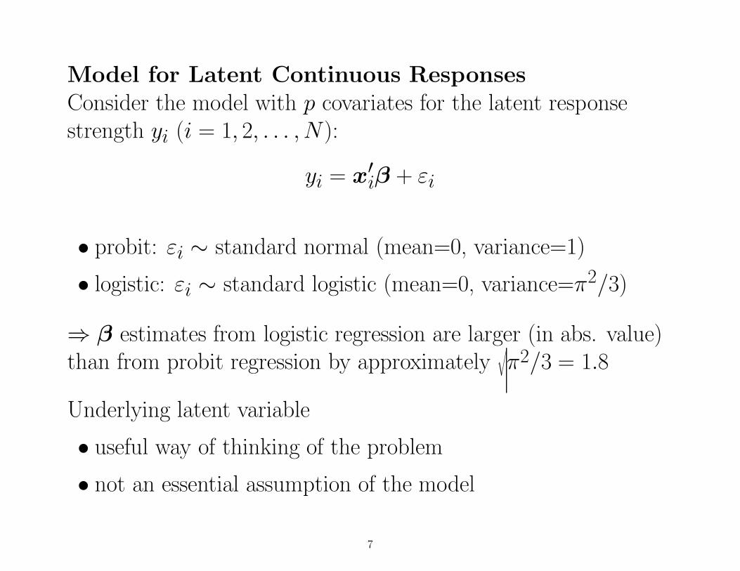
Model for Latent Continuous ResponsesConsider the model with p covariates for the latent responsestrength yi (i = 1, 2, . . . , N):
yi = x′iβ + εi
• probit: εi ∼ standard normal (mean=0, variance=1)
• logistic: εi ∼ standard logistic (mean=0, variance=π2/3)
⇒ β estimates from logistic regression are larger (in abs. value)than from probit regression by approximately
√
π2/3 = 1.8
Underlying latent variable
• useful way of thinking of the problem
• not an essential assumption of the model
7
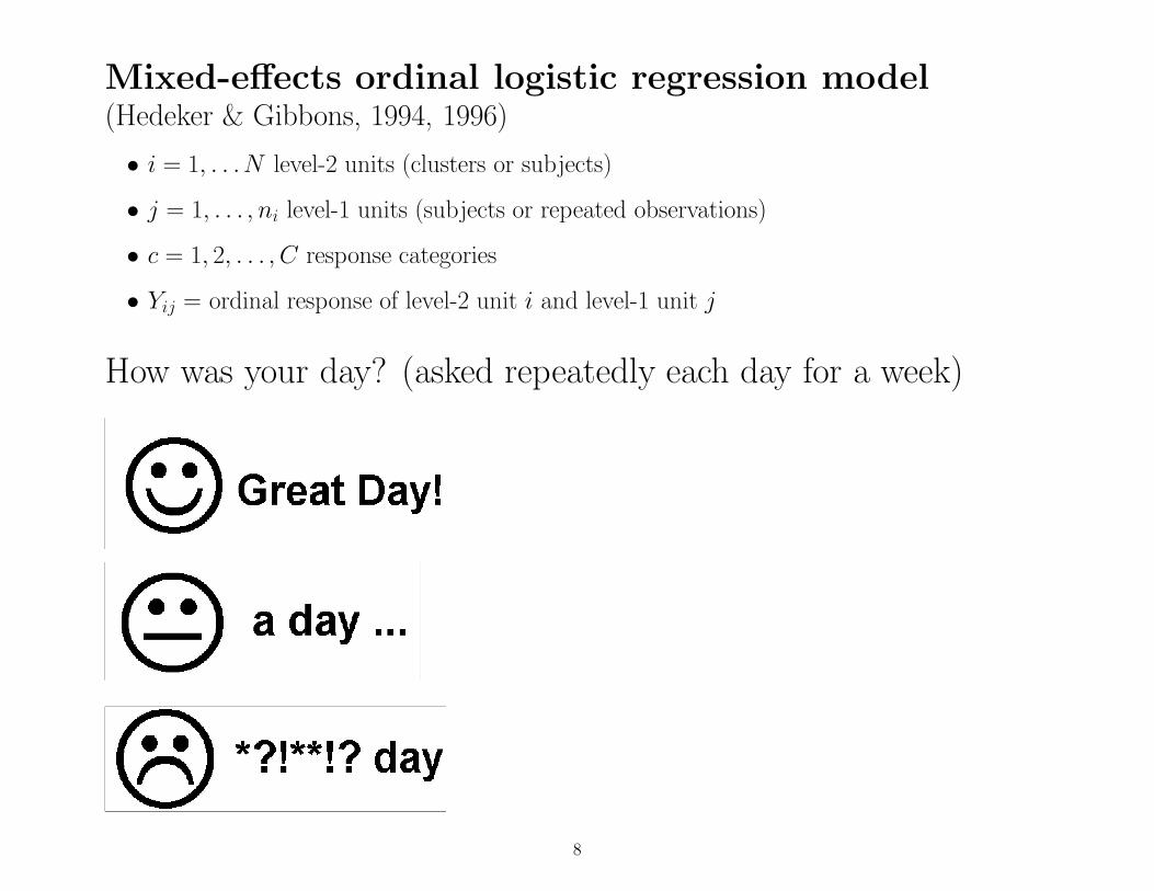
Mixed-effects ordinal logistic regression model(Hedeker & Gibbons, 1994, 1996)
• i = 1, . . .N level-2 units (clusters or subjects)
• j = 1, . . . , ni level-1 units (subjects or repeated observations)
• c = 1, 2, . . . , C response categories
• Yij = ordinal response of level-2 unit i and level-1 unit j
How was your day? (asked repeatedly each day for a week)
8
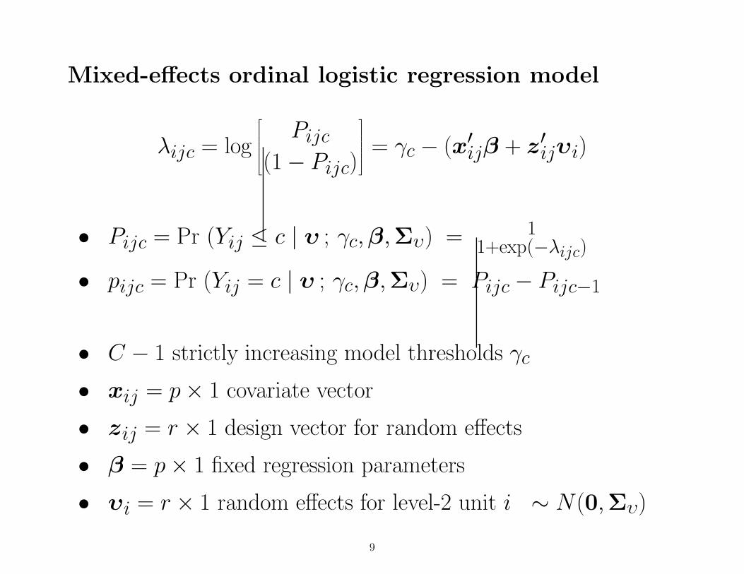
Mixed-effects ordinal logistic regression model
λijc = log
Pijc
(1 − Pijc)
= γc − (x′
ijβ + z′ijυi)
• Pijc = Pr (Yij ≤ c | υ ; γc,β,Συ) = 11+exp(−λijc)
• pijc = Pr (Yij = c | υ ; γc,β,Συ) = Pijc − Pijc−1
• C − 1 strictly increasing model thresholds γc
• xij = p × 1 covariate vector
• zij = r × 1 design vector for random effects
• β = p × 1 fixed regression parameters
• υi = r × 1 random effects for level-2 unit i ∼ N(0,Συ)
9
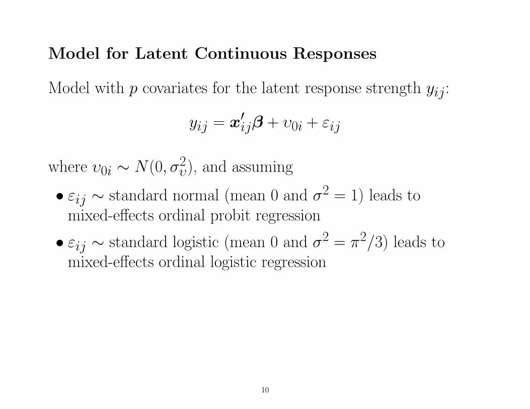
Model for Latent Continuous Responses
Model with p covariates for the latent response strength yij:
yij = x′ijβ + υ0i + εij
where υ0i ∼ N(0, σ2υ), and assuming
• εij ∼ standard normal (mean 0 and σ2 = 1) leads tomixed-effects ordinal probit regression
• εij ∼ standard logistic (mean 0 and σ2 = π2/3) leads tomixed-effects ordinal logistic regression
10
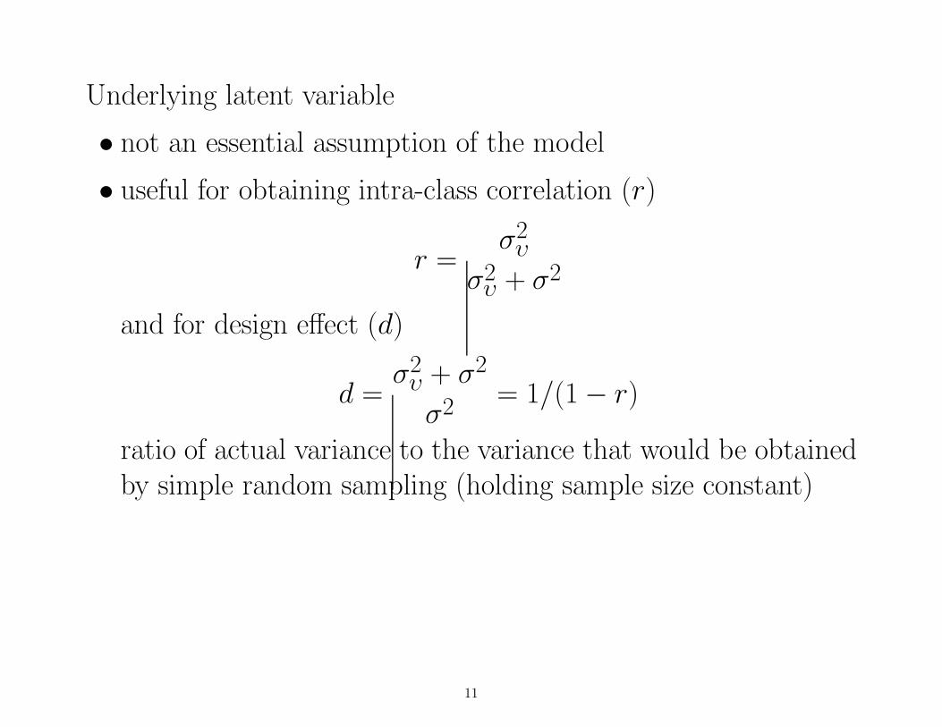
Underlying latent variable
• not an essential assumption of the model
• useful for obtaining intra-class correlation (r)
r =σ2υ
σ2υ + σ2
and for design effect (d)
d =σ2υ + σ2
σ2 = 1/(1 − r)
ratio of actual variance to the variance that would be obtainedby simple random sampling (holding sample size constant)
11
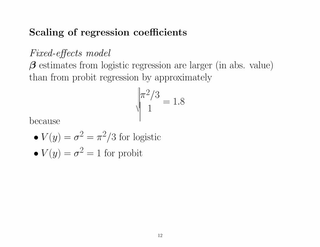
Scaling of regression coefficients
Fixed-effects modelβ estimates from logistic regression are larger (in abs. value)than from probit regression by approximately
√√√√√√√√π2/3
1= 1.8
because
• V (y) = σ2 = π2/3 for logistic
• V (y) = σ2 = 1 for probit
12
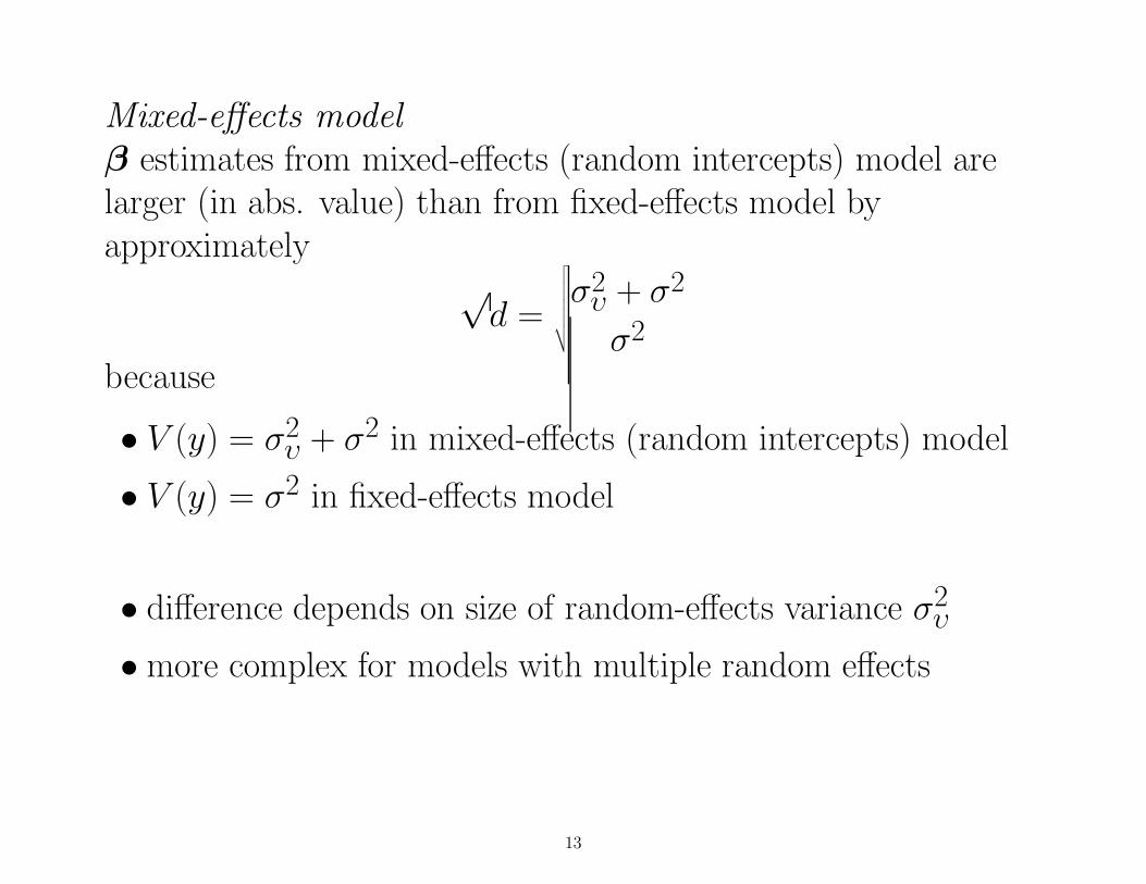
Mixed-effects modelβ estimates from mixed-effects (random intercepts) model arelarger (in abs. value) than from fixed-effects model byapproximately
√d =
√√√√√√√√σ2υ + σ2
σ2
because
• V (y) = σ2υ + σ2 in mixed-effects (random intercepts) model
• V (y) = σ2 in fixed-effects model
• difference depends on size of random-effects variance σ2υ
• more complex for models with multiple random effects
13
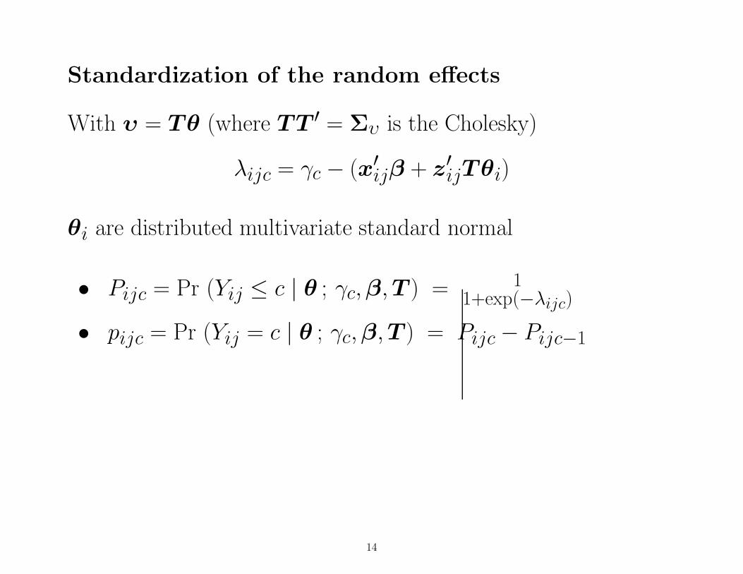
Standardization of the random effects
With υ = Tθ (where TT ′ = Συ is the Cholesky)
λijc = γc − (x′ijβ + z′ijTθi)
θi are distributed multivariate standard normal
• Pijc = Pr (Yij ≤ c | θ ; γc,β,T ) = 11+exp(−λijc)
• pijc = Pr (Yij = c | θ ; γc,β,T ) = Pijc − Pijc−1
14
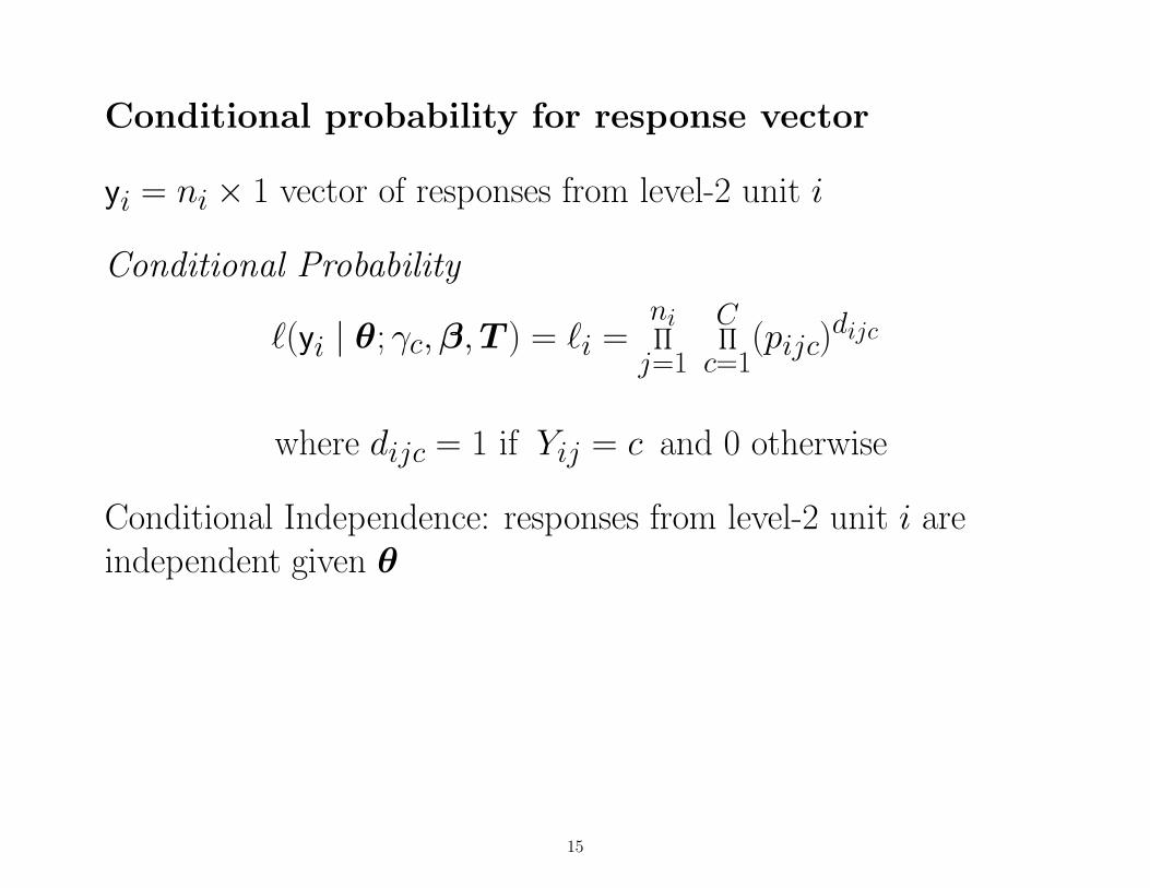
Conditional probability for response vector
yi = ni × 1 vector of responses from level-2 unit i
Conditional Probability
`(yi | θ; γc,β,T ) = `i =ni∏
j=1
C∏
c=1(pijc)
dijc
where dijc = 1 if Yij = c and 0 otherwise
Conditional Independence: responses from level-2 unit i areindependent given θ
15

Maximum (Marginal) Likelihood Estimation
Marginal Probability
h(yi) = hi =∫
θ `i g(θ) dθ
g(θ) = multivariate standard normal density
Maximize the marginal log-likelihood from N level-2 units
log L =N∑
ilog hi with respect to η = [ γc
... β ... T ]
Full-likelihood approach found in SAS PROC NLMIXED &GLIMMIX, STATA, SUPERMIX, MIXOR
16
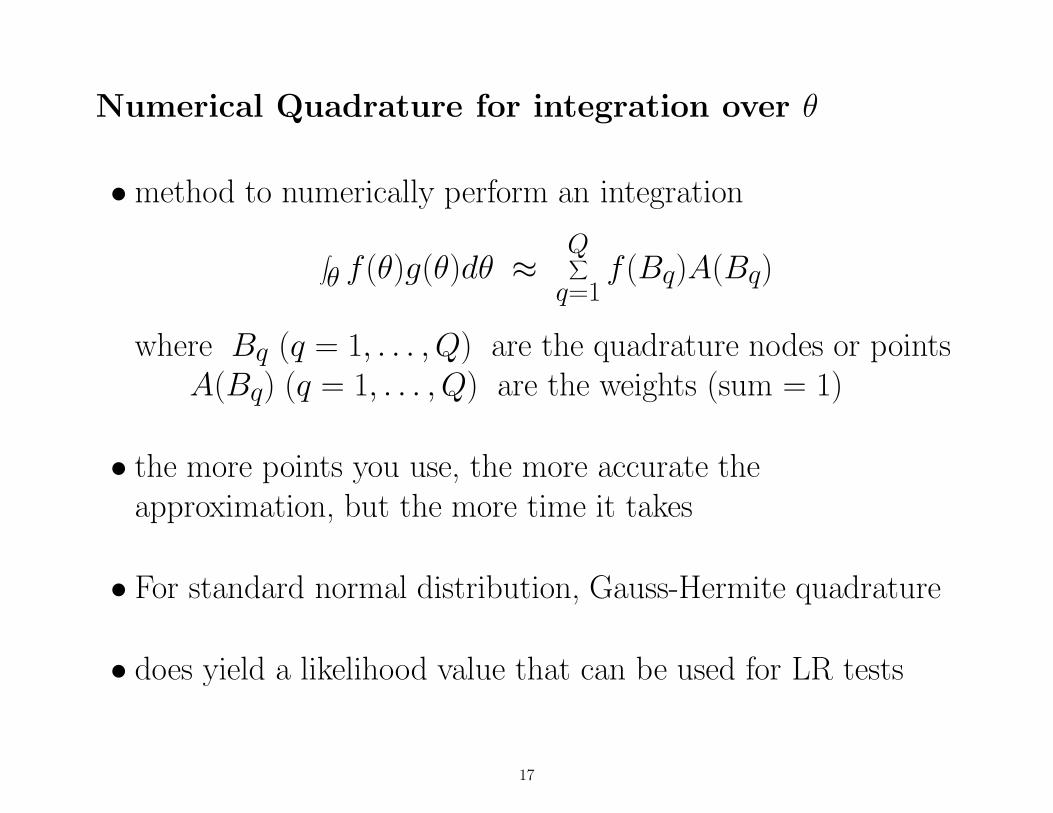
Numerical Quadrature for integration over θ
• method to numerically perform an integration
∫
θ f(θ)g(θ)dθ ≈Q∑
q=1f(Bq)A(Bq)
where Bq (q = 1, . . . , Q) are the quadrature nodes or pointsA(Bq) (q = 1, . . . , Q) are the weights (sum = 1)
• the more points you use, the more accurate theapproximation, but the more time it takes
• For standard normal distribution, Gauss-Hermite quadrature
• does yield a likelihood value that can be used for LR tests
17
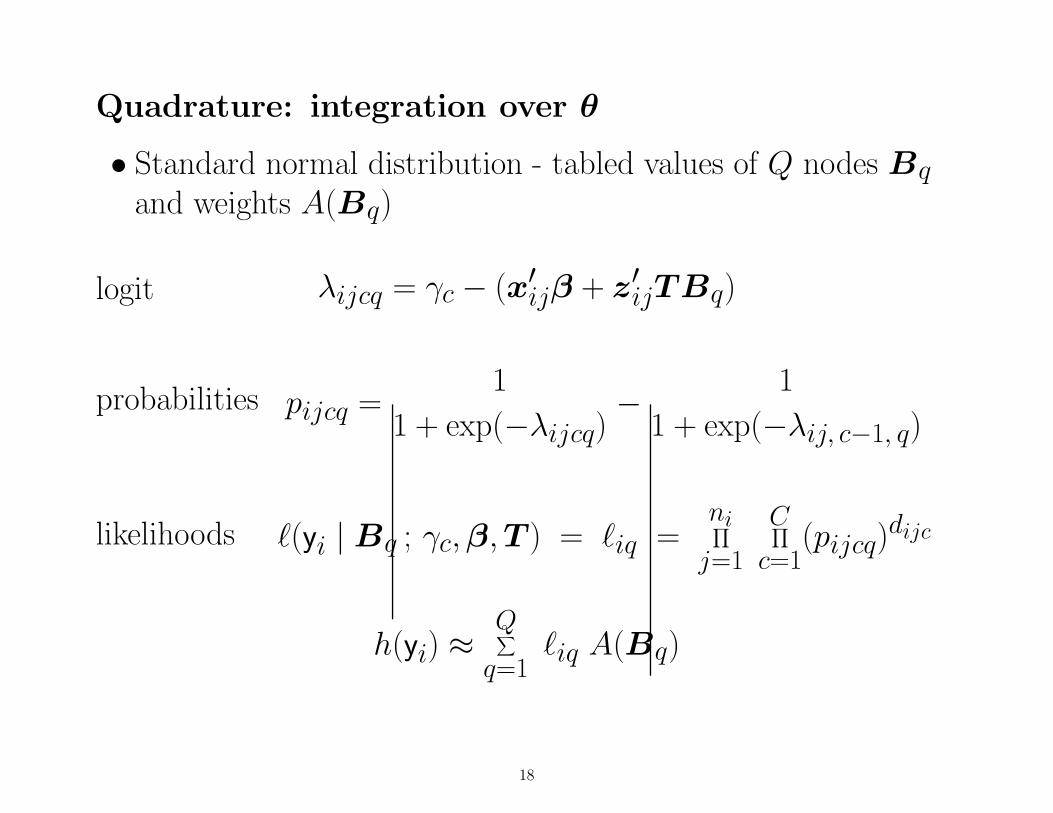
Quadrature: integration over θ
• Standard normal distribution - tabled values of Q nodes Bq
and weights A(Bq)
logit λijcq = γc − (x′ijβ + z′ijTBq)
probabilities pijcq =1
1 + exp(−λijcq)− 1
1 + exp(−λij, c−1, q)
likelihoods `(yi | Bq ; γc,β,T ) = `iq =ni∏
j=1
C∏
c=1(pijcq)
dijc
h(yi) ≈Q∑
q=1`iq A(Bq)
18

Empirical Bayes estimates (univariate case)
θi = E(θi | yi) =1
hi
∫
θ θi `i g(θ) dθ ≈ 1
hi
Q∑
q=1Bq `iq A(Bq)
The variance of this estimator is obtained as:
V (θi | yi) =1
hi
∫
θ (θi − θi)2 `i g(θ) dθ
≈ 1
hi
Q∑
q=1(Bq − θi)
2 `iq A(Bq)
At convergence, one more round of quadrature and the values of
• hi = h(yi) which vary by i units
• `iq = `(yi | Bq ; γc,β, συ) which vary by i units and quad pts
19
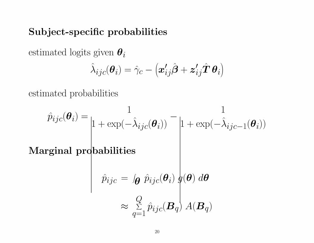
Subject-specific probabilities
estimated logits given θi
λijc(θi) = γc −x′
ijβ + z′ijT θi
estimated probabilities
pijc(θi) =1
1 + exp(−λijc(θi))− 1
1 + exp(−λijc−1(θi))
Marginal probabilities
pijc =∫
θ pijc(θi) g(θ) dθ
≈Q∑
q=1pijc(Bq) A(Bq)
20
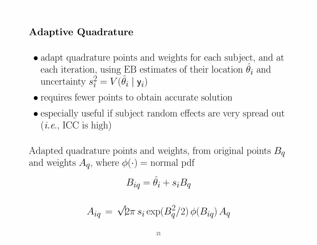
Adaptive Quadrature
• adapt quadrature points and weights for each subject, and ateach iteration, using EB estimates of their location θi anduncertainty s2
i = V (θi | yi)
• requires fewer points to obtain accurate solution
• especially useful if subject random effects are very spread out(i.e., ICC is high)
Adapted quadrature points and weights, from original points Bq
and weights Aq, where φ(·) = normal pdf
Biq = θi + siBq
Aiq =√
2π si exp(B2q/2) φ(Biq) Aq
21

Multiple Random Effects
• quadrature solution must integrate over each random effectdimension (r = number of random effects)
Bq = (Bq1, Bq2, . . . , Bqr) = r − dimension quad pt vector
A(Bq) =r∏
h=1A(Bqh) = product of univariate weights
• curse of dimensionality: Qr total points, where Q is thenumber of points per dimension (e.g., Q = 10 and r = 3 leadsto evaluation at 1000 points)
• adaptive quadrature especially useful here, since Q can belower
22
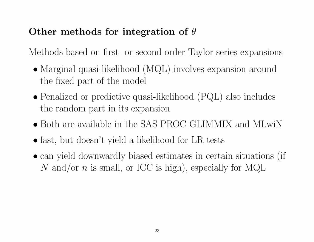
Other methods for integration of θ
Methods based on first- or second-order Taylor series expansions
• Marginal quasi-likelihood (MQL) involves expansion aroundthe fixed part of the model
• Penalized or predictive quasi-likelihood (PQL) also includesthe random part in its expansion
• Both are available in the SAS PROC GLIMMIX and MLwiN
• fast, but doesn’t yield a likelihood for LR tests
• can yield downwardly biased estimates in certain situations (ifN and/or n is small, or ICC is high), especially for MQL
23
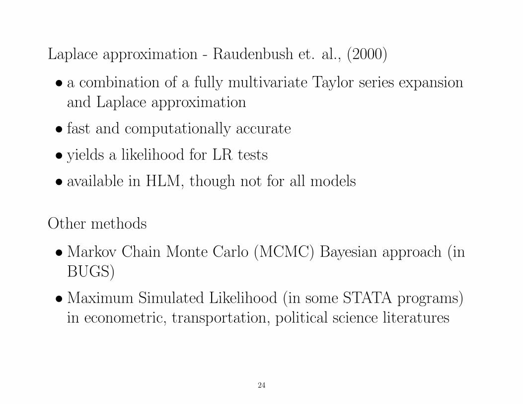
Laplace approximation - Raudenbush et. al., (2000)
• a combination of a fully multivariate Taylor series expansionand Laplace approximation
• fast and computationally accurate
• yields a likelihood for LR tests
• available in HLM, though not for all models
Other methods
• Markov Chain Monte Carlo (MCMC) Bayesian approach (inBUGS)
• Maximum Simulated Likelihood (in some STATA programs)in econometric, transportation, political science literatures
24

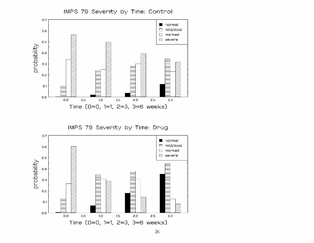
Treatment-Related Change Across Time
Data from the NIMH Schizophrenia collaborative study on treatment relatedchanges in overall severity. IMPS item 79, Severity of Illness, was scored as:
1 = normal or borderline mentally ill2 = mildly or moderately ill3 = markedly ill4 = severely or among the most extremely ill
The experimental design and corresponding sample sizes:
Sample size at WeekGroup 0 1 2 3 4 5 6 completersPLC (n=108) 107 105 5 87 2 2 70 65%DRUG (n=329) 327 321 9 287 9 7 265 81%Drug = Chlorpromazine, Fluphenazine, or Thioridazine
Main question of interest:
• Was there differential improvement for the drug groups relative to thecontrol group?
25
26
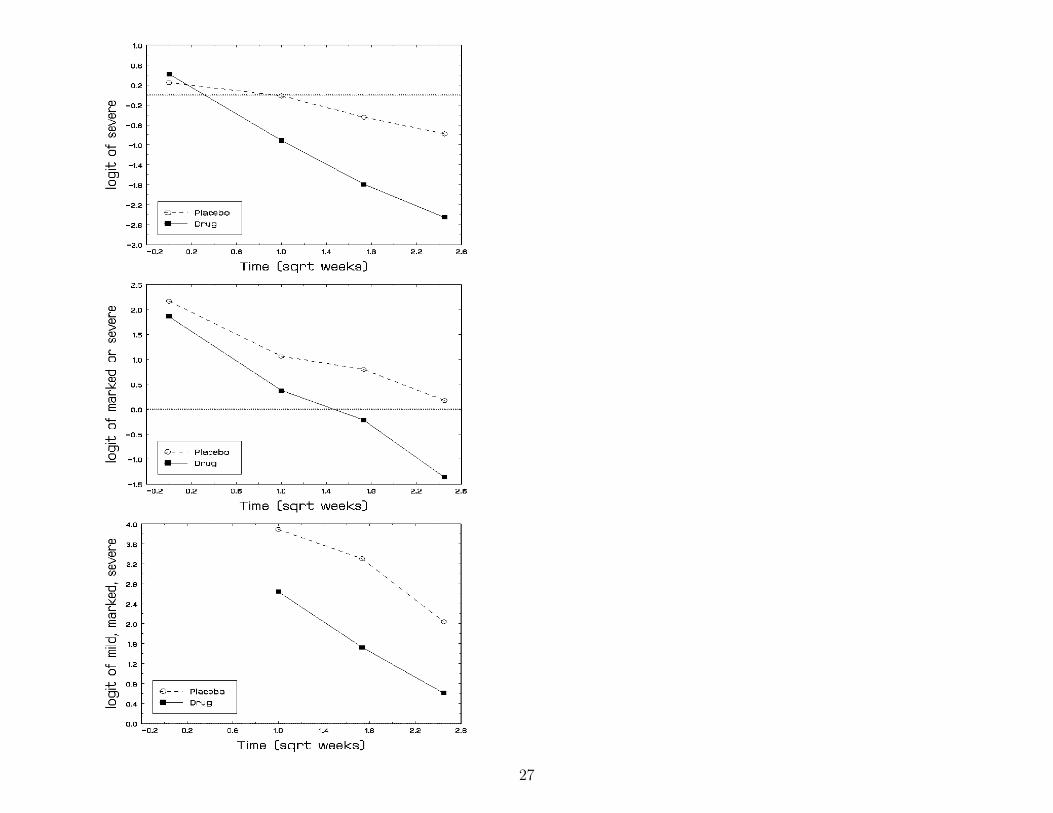
27

Within-Subjects / Between-Subjects components
Within-subjects model - level 1 (j = 1, . . . , ni obs)
λijc = γc − [b0i + b1i
√Weekj]
Between-subjects model - level 2 (i = 1, . . . , N subjects)
b0i = β0 + β2Grpi + υ0i
b1i = β1 + β3Grpi
υ0i ∼ NID(0, σ2υ)
28
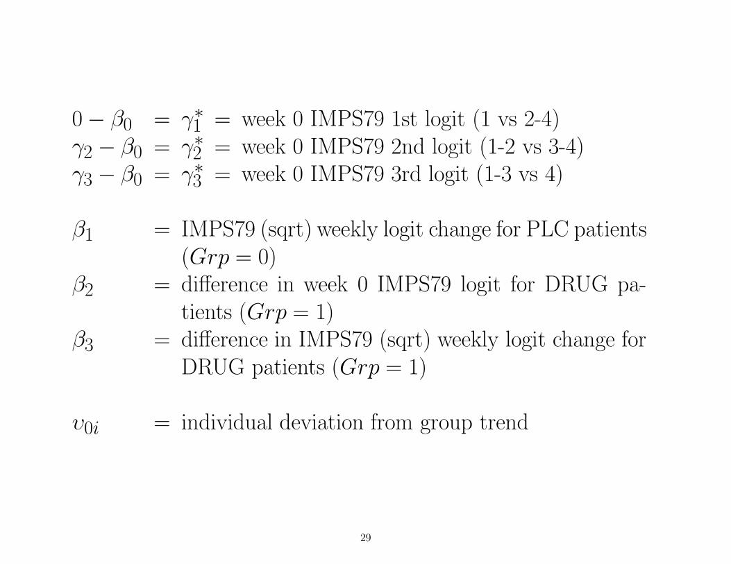
0 − β0 = γ∗1 = week 0 IMPS79 1st logit (1 vs 2-4)γ2 − β0 = γ∗2 = week 0 IMPS79 2nd logit (1-2 vs 3-4)γ3 − β0 = γ∗3 = week 0 IMPS79 3rd logit (1-3 vs 4)
β1 = IMPS79 (sqrt) weekly logit change for PLC patients(Grp = 0)
β2 = difference in week 0 IMPS79 logit for DRUG pa-tients (Grp = 1)
β3 = difference in IMPS79 (sqrt) weekly logit change forDRUG patients (Grp = 1)
υ0i = individual deviation from group trend
29
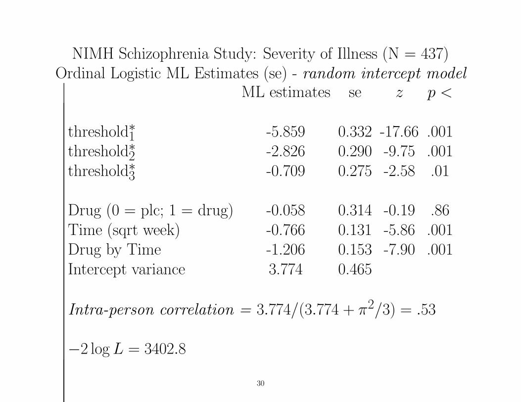
NIMH Schizophrenia Study: Severity of Illness (N = 437)Ordinal Logistic ML Estimates (se) - random intercept model
ML estimates se z p <
threshold∗1 -5.859 0.332 -17.66 .001threshold∗2 -2.826 0.290 -9.75 .001threshold∗3 -0.709 0.275 -2.58 .01
Drug (0 = plc; 1 = drug) -0.058 0.314 -0.19 .86Time (sqrt week) -0.766 0.131 -5.86 .001Drug by Time -1.206 0.153 -7.90 .001Intercept variance 3.774 0.465
Intra-person correlation = 3.774/(3.774 + π2/3) = .53
−2 log L = 3402.8
30

Within-Subjects / Between-Subjects components
Within-subjects model - level 1 (j = 1, . . . , ni obs)
logitcij = γc − [b0i + b1i
√Weekj]
Between-subjects model - level 2 (i = 1, . . . , N subjects)
b0i = β0 + β2Grpi + υ0i
b1i = β1 + β3Grpi + υ1i
υi ∼ NID(0,Σ)
31
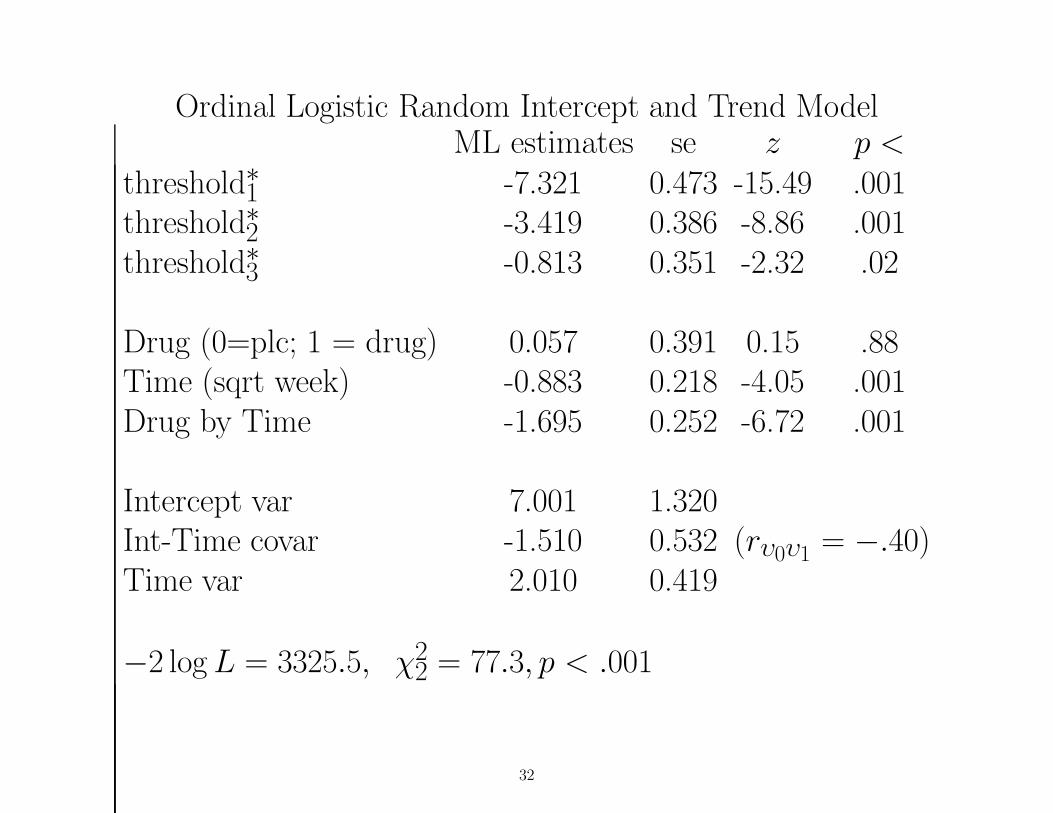
Ordinal Logistic Random Intercept and Trend ModelML estimates se z p <
threshold∗1 -7.321 0.473 -15.49 .001threshold∗2 -3.419 0.386 -8.86 .001threshold∗3 -0.813 0.351 -2.32 .02
Drug (0=plc; 1 = drug) 0.057 0.391 0.15 .88Time (sqrt week) -0.883 0.218 -4.05 .001Drug by Time -1.695 0.252 -6.72 .001
Intercept var 7.001 1.320Int-Time covar -1.510 0.532 (rυ0υ1 = −.40)Time var 2.010 0.419
−2 log L = 3325.5, χ22 = 77.3, p < .001
32
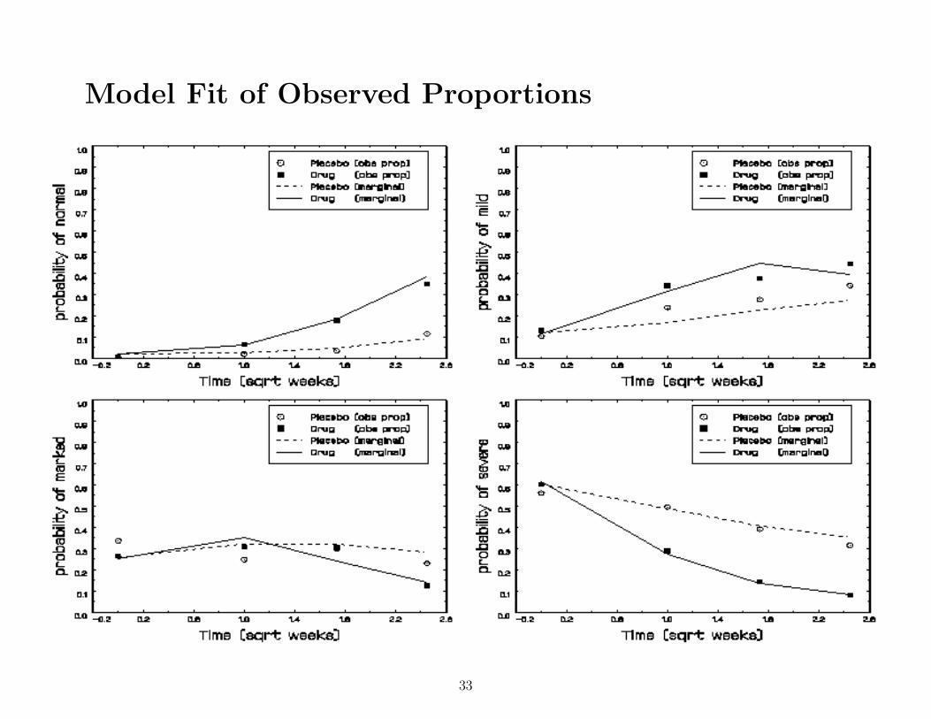
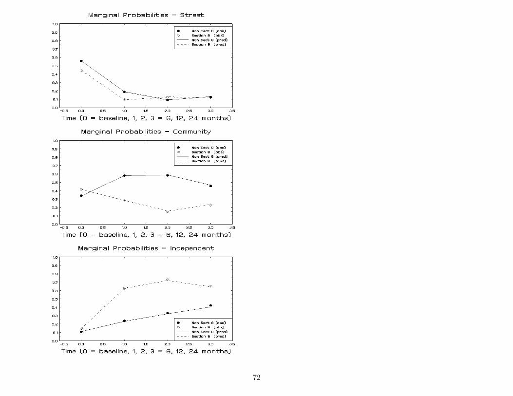
Model Fit of Observed Proportions
33
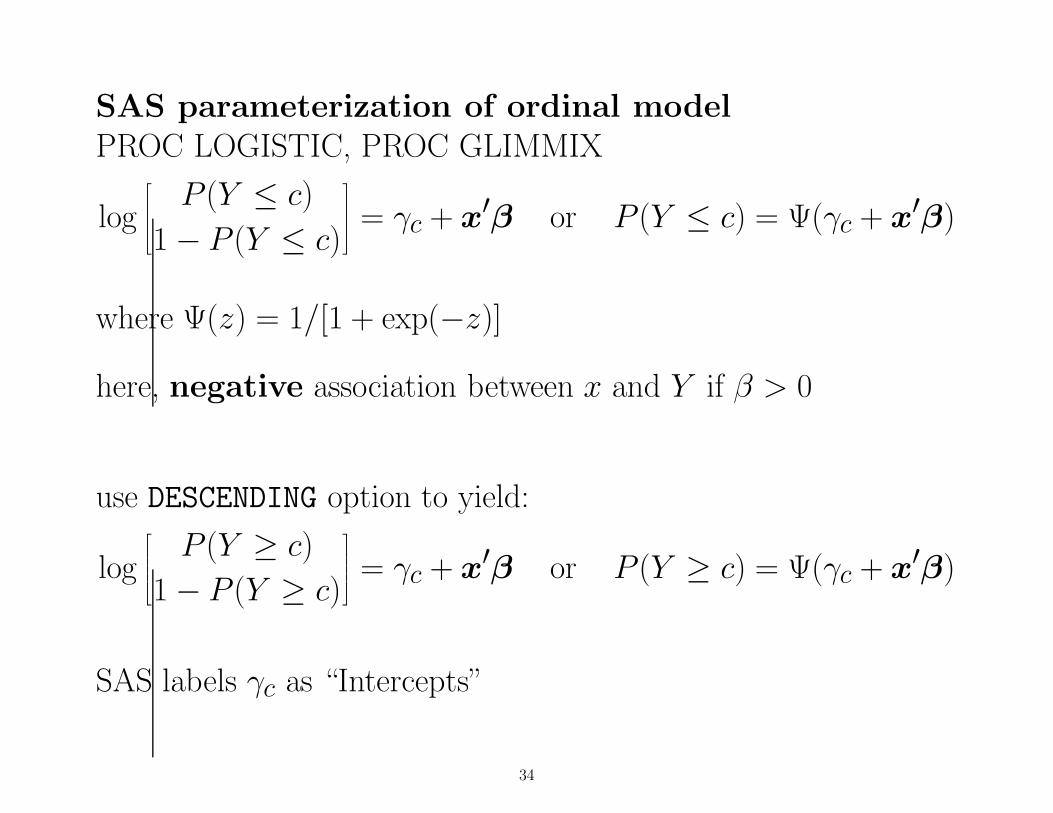
SAS parameterization of ordinal modelPROC LOGISTIC, PROC GLIMMIX
log
P (Y ≤ c)
1 − P (Y ≤ c)
= γc + x′β or P (Y ≤ c) = Ψ(γc + x′β)
where Ψ(z) = 1/[1 + exp(−z)]
here, negative association between x and Y if β > 0
use DESCENDING option to yield:
log
P (Y ≥ c)
1 − P (Y ≥ c)
= γc + x′β or P (Y ≥ c) = Ψ(γc + x′β)
SAS labels γc as “Intercepts”
34
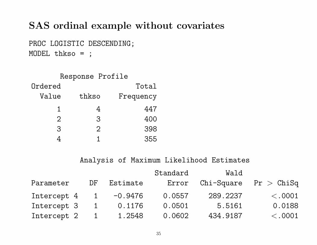
SAS ordinal example without covariates
PROC LOGISTIC DESCENDING;
MODEL thkso = ;
Response Profile
Ordered Total
Value thkso Frequency
1 4 447
2 3 400
3 2 398
4 1 355
Analysis of Maximum Likelihood Estimates
Standard Wald
Parameter DF Estimate Error Chi-Square Pr > ChiSq
Intercept 4 1 -0.9476 0.0557 289.2237 <.0001
Intercept 3 1 0.1176 0.0501 5.5161 0.0188
Intercept 2 1 1.2548 0.0602 434.9187 <.0001
35
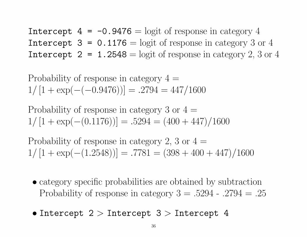
Intercept 4 = -0.9476 = logit of response in category 4Intercept 3 = 0.1176 = logit of response in category 3 or 4Intercept 2 = 1.2548 = logit of response in category 2, 3 or 4
Probability of response in category 4 =1/ [1 + exp(−(−0.9476))] = .2794 = 447/1600
Probability of response in category 3 or 4 =1/ [1 + exp(−(0.1176))] = .5294 = (400 + 447)/1600
Probability of response in category 2, 3 or 4 =1/ [1 + exp(−(1.2548))] = .7781 = (398 + 400 + 447)/1600
• category specific probabilities are obtained by subtractionProbability of response in category 3 = .5294 - .2794 = .25
• Intercept 2 > Intercept 3 > Intercept 4
36
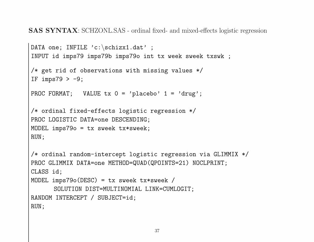
SAS SYNTAX: SCHZONL.SAS - ordinal fixed- and mixed-effects logistic regression
DATA one; INFILE ’c:\schizx1.dat’ ;
INPUT id imps79 imps79b imps79o int tx week sweek txswk ;
/* get rid of observations with missing values */
IF imps79 > -9;
PROC FORMAT; VALUE tx 0 = ’placebo’ 1 = ’drug’;
/* ordinal fixed-effects logistic regression */
PROC LOGISTIC DATA=one DESCENDING;
MODEL imps79o = tx sweek tx*sweek;
RUN;
/* ordinal random-intercept logistic regression via GLIMMIX */
PROC GLIMMIX DATA=one METHOD=QUAD(QPOINTS=21) NOCLPRINT;
CLASS id;
MODEL imps79o(DESC) = tx sweek tx*sweek /
SOLUTION DIST=MULTINOMIAL LINK=CUMLOGIT;
RANDOM INTERCEPT / SUBJECT=id;
RUN;
37
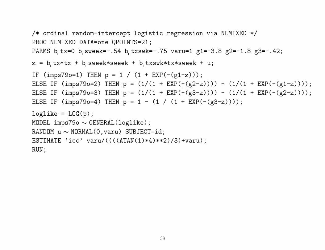
/* ordinal random-intercept logistic regression via NLMIXED */
PROC NLMIXED DATA=one QPOINTS=21;
PARMS b tx=0 b sweek=-.54 b txswk=-.75 varu=1 g1=-3.8 g2=-1.8 g3=-.42;
z = b tx*tx + b sweek*sweek + b txswk*tx*sweek + u;
IF (imps79o=1) THEN p = 1 / (1 + EXP(-(g1-z)));
ELSE IF (imps79o=2) THEN p = (1/(1 + EXP(-(g2-z)))) - (1/(1 + EXP(-(g1-z))));
ELSE IF (imps79o=3) THEN p = (1/(1 + EXP(-(g3-z)))) - (1/(1 + EXP(-(g2-z))));
ELSE IF (imps79o=4) THEN p = 1 - (1 / (1 + EXP(-(g3-z))));
loglike = LOG(p);
MODEL imps79o ∼ GENERAL(loglike);
RANDOM u ∼ NORMAL(0,varu) SUBJECT=id;
ESTIMATE ’icc’ varu/((((ATAN(1)*4)**2)/3)+varu);
RUN;
38
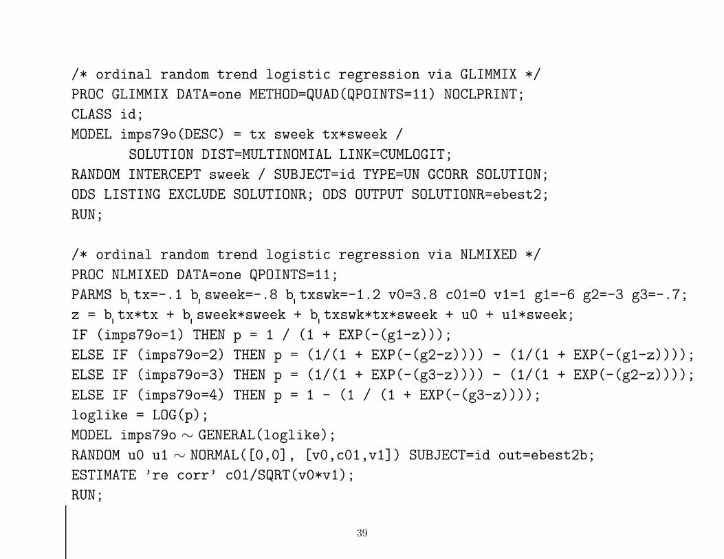
/* ordinal random trend logistic regression via GLIMMIX */
PROC GLIMMIX DATA=one METHOD=QUAD(QPOINTS=11) NOCLPRINT;
CLASS id;
MODEL imps79o(DESC) = tx sweek tx*sweek /
SOLUTION DIST=MULTINOMIAL LINK=CUMLOGIT;
RANDOM INTERCEPT sweek / SUBJECT=id TYPE=UN GCORR SOLUTION;
ODS LISTING EXCLUDE SOLUTIONR; ODS OUTPUT SOLUTIONR=ebest2;
RUN;
/* ordinal random trend logistic regression via NLMIXED */
PROC NLMIXED DATA=one QPOINTS=11;
PARMS b tx=-.1 b sweek=-.8 b txswk=-1.2 v0=3.8 c01=0 v1=1 g1=-6 g2=-3 g3=-.7;
z = b tx*tx + b sweek*sweek + b txswk*tx*sweek + u0 + u1*sweek;
IF (imps79o=1) THEN p = 1 / (1 + EXP(-(g1-z)));
ELSE IF (imps79o=2) THEN p = (1/(1 + EXP(-(g2-z)))) - (1/(1 + EXP(-(g1-z))));
ELSE IF (imps79o=3) THEN p = (1/(1 + EXP(-(g3-z)))) - (1/(1 + EXP(-(g2-z))));
ELSE IF (imps79o=4) THEN p = 1 - (1 / (1 + EXP(-(g3-z))));
loglike = LOG(p);
MODEL imps79o ∼ GENERAL(loglike);
RANDOM u0 u1 ∼ NORMAL([0,0], [v0,c01,v1]) SUBJECT=id out=ebest2b;
ESTIMATE ’re corr’ c01/SQRT(v0*v1);
RUN;
39

Model fit of observed marginal proportions
1. yi = Xi β
2. calculate “marginalization” vector
s =1
σ
Diag(V (yi))
1/2
• V (yi) = ZiΣZ′i + σ2Ii
• σ = 1 for probit and σ = π/√
3 for logistic
• Zi = design matrix for random effects
• for random-intercepts model Zi = 1i, and so,s =
√
σ2υ/σ2 + 1
40
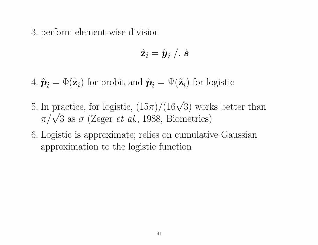
3. perform element-wise division
zi = yi /. s
4. pi = Φ(zi) for probit and pi = Ψ(zi) for logistic
5. In practice, for logistic, (15π)/(16√
3) works better thanπ/
√3 as σ (Zeger et al., 1988, Biometrics)
6. Logistic is approximate; relies on cumulative Gaussianapproximation to the logistic function
41
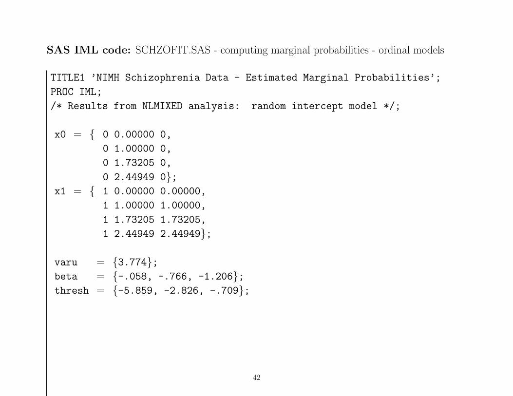
SAS IML code: SCHZOFIT.SAS - computing marginal probabilities - ordinal models
TITLE1 ’NIMH Schizophrenia Data - Estimated Marginal Probabilities’;
PROC IML;
/* Results from NLMIXED analysis: random intercept model */;
x0 = { 0 0.00000 0,
0 1.00000 0,
0 1.73205 0,
0 2.44949 0};x1 = { 1 0.00000 0.00000,
1 1.00000 1.00000,
1 1.73205 1.73205,
1 2.44949 2.44949};
varu = {3.774};beta = {-.058, -.766, -1.206};thresh = {-5.859, -2.826, -.709};
42

/* Approximate Marginalization Method */;
pi = ATAN(1)*4;
nt = 4;
ivec = J(nt,1,1);
zvec = J(nt,1,1);
evec = (15/16)**2 * (pi**2)/3 * ivec;
/* nt by nt matrix with evec on the diagonal and zeros elsewhere */;
emat = diag(evec);
/* variance-covariance matrix of underlying latent variable */;
vary = zvec * varu * T(zvec) + emat;
sdy = sqrt(vecdiag(vary) / vecdiag(emat));
43
za0 = (thresh[1] - x0*beta) / sdy ;
zb0 = (thresh[2] - x0*beta) / sdy;
zc0 = (thresh[3] - x0*beta) / sdy;
za1 = (thresh[1] - x1*beta) / sdy;
zb1 = (thresh[2] - x1*beta) / sdy;
zc1 = (thresh[3] - x1*beta) / sdy;
grp0a = 1 / ( 1 + EXP(- za0));
grp0b = 1 / ( 1 + EXP(- zb0));
grp0c = 1 / ( 1 + EXP(- zc0));
grp1a = 1 / ( 1 + EXP(- za1));
grp1b = 1 / ( 1 + EXP(- zb1));
grp1c = 1 / ( 1 + EXP(- zc1));
print ’Random intercept model’;
print ’Approximate Marginalization Method’;
print ’marginal prob for group 0 - catg 1’ grp0a [FORMAT=8.4];
print ’marginal prob for group 0 - catg 2’ (grp0b-grp0a) [FORMAT=8.4];
print ’marginal prob for group 0 - catg 3’ (grp0c-grp0b) [FORMAT=8.4];
print ’marginal prob for group 0 - catg 4’ (1-grp0c) [FORMAT=8.4];
print ’marginal prob for group 1 - catg 1’ grp1a [FORMAT=8.4];
print ’marginal prob for group 1 - catg 2’ (grp1b-grp1a) [FORMAT=8.4];
print ’marginal prob for group 1 - catg 3’ (grp1c-grp1b) [FORMAT=8.4];
print ’marginal prob for group 1 - catg 4’ (1-grp1c) [FORMAT=8.4];
44
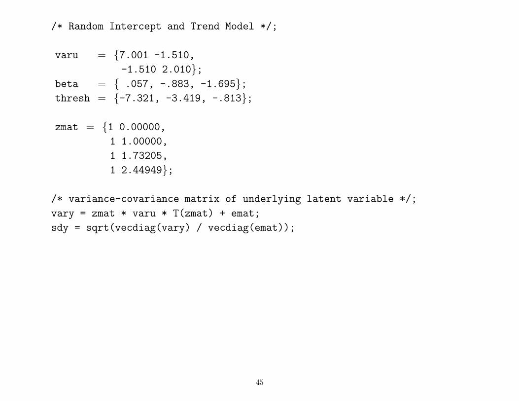
/* Random Intercept and Trend Model */;
varu = {7.001 -1.510,
-1.510 2.010};beta = { .057, -.883, -1.695};thresh = {-7.321, -3.419, -.813};
zmat = {1 0.00000,
1 1.00000,
1 1.73205,
1 2.44949};
/* variance-covariance matrix of underlying latent variable */;
vary = zmat * varu * T(zmat) + emat;
sdy = sqrt(vecdiag(vary) / vecdiag(emat));
45
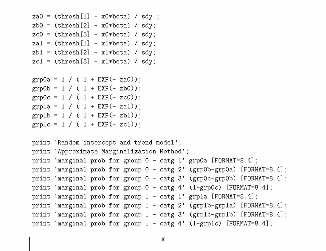
za0 = (thresh[1] - x0*beta) / sdy ;
zb0 = (thresh[2] - x0*beta) / sdy;
zc0 = (thresh[3] - x0*beta) / sdy;
za1 = (thresh[1] - x1*beta) / sdy;
zb1 = (thresh[2] - x1*beta) / sdy;
zc1 = (thresh[3] - x1*beta) / sdy;
grp0a = 1 / ( 1 + EXP(- za0));
grp0b = 1 / ( 1 + EXP(- zb0));
grp0c = 1 / ( 1 + EXP(- zc0));
grp1a = 1 / ( 1 + EXP(- za1));
grp1b = 1 / ( 1 + EXP(- zb1));
grp1c = 1 / ( 1 + EXP(- zc1));
print ’Random intercept and trend model’;
print ’Approximate Marginalization Method’;
print ’marginal prob for group 0 - catg 1’ grp0a [FORMAT=8.4];
print ’marginal prob for group 0 - catg 2’ (grp0b-grp0a) [FORMAT=8.4];
print ’marginal prob for group 0 - catg 3’ (grp0c-grp0b) [FORMAT=8.4];
print ’marginal prob for group 0 - catg 4’ (1-grp0c) [FORMAT=8.4];
print ’marginal prob for group 1 - catg 1’ grp1a [FORMAT=8.4];
print ’marginal prob for group 1 - catg 2’ (grp1b-grp1a) [FORMAT=8.4];
print ’marginal prob for group 1 - catg 3’ (grp1c-grp1b) [FORMAT=8.4];
print ’marginal prob for group 1 - catg 4’ (1-grp1c) [FORMAT=8.4];
46

Proportional and Non-proportional Odds
Proportional Odds model
log
P (Yij ≤ c)
1 − P (Yij ≤ c)
= γc −
[
x′ijβ + z′ijυi
]
with υi ∼ N(0,TT ′ = Σ)
= γc −[
x′ijβ + z′ijTθi
]
with θi ∼ N(0, I)
• relationship between the explanatory variables and thecumulative logits does not depend on c
• effects of x variables DO NOT vary across the C − 1cumulative logits
47
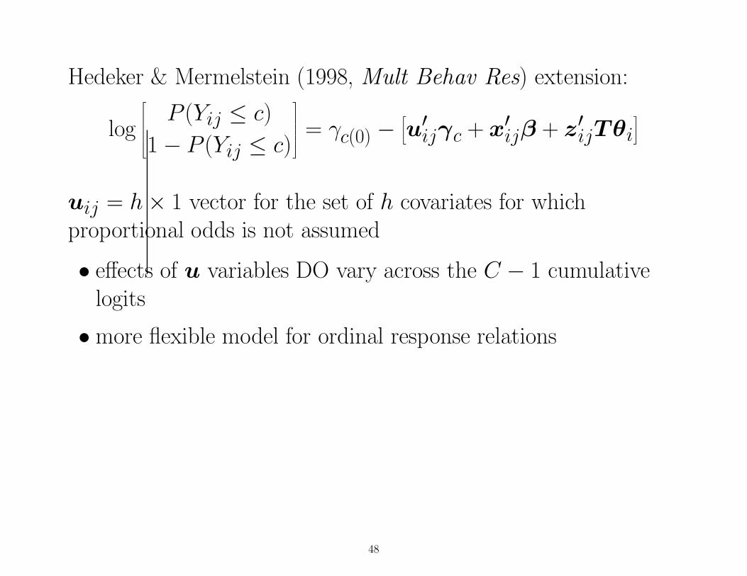
Hedeker & Mermelstein (1998, Mult Behav Res) extension:
log
P (Yij ≤ c)
1 − P (Yij ≤ c)
= γc(0) −
[
u′ijγc + x′
ijβ + z′ijTθi]
uij = h × 1 vector for the set of h covariates for whichproportional odds is not assumed
• effects of u variables DO vary across the C − 1 cumulativelogits
• more flexible model for ordinal response relations
48
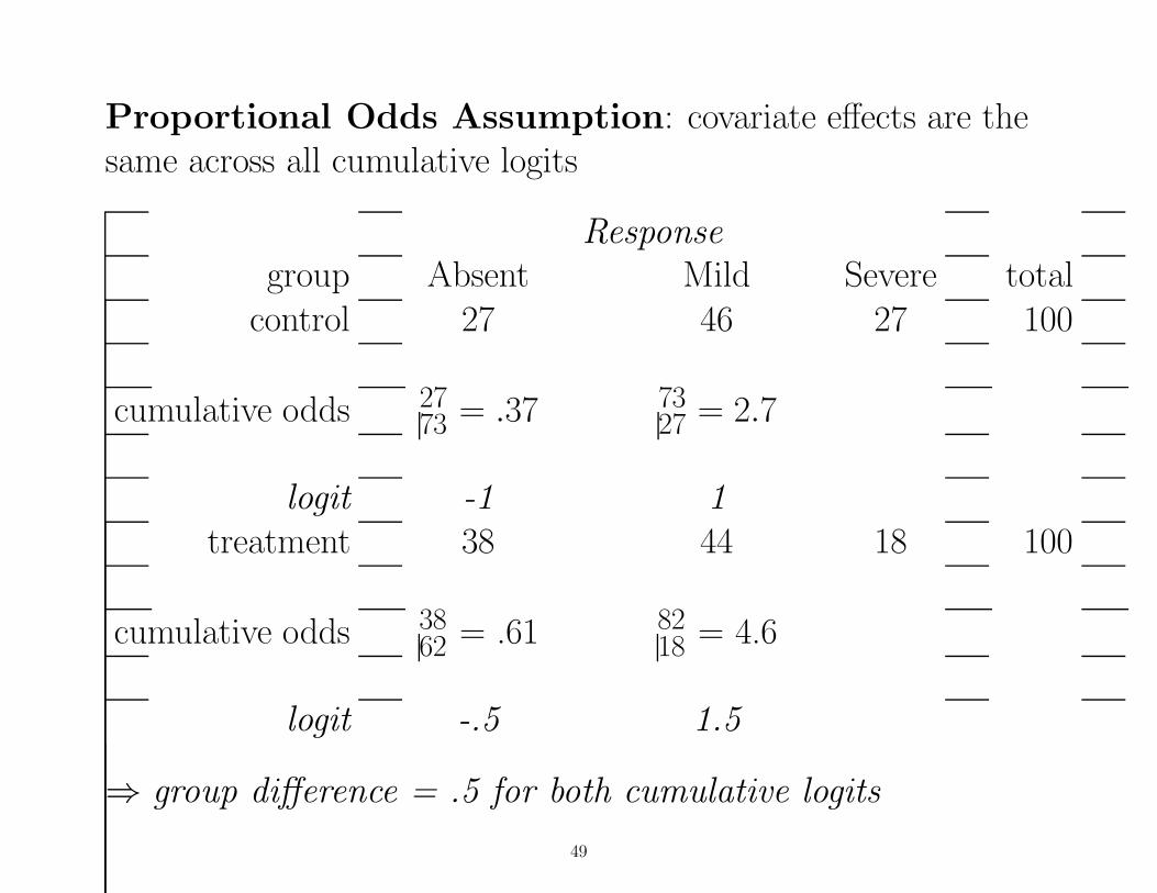
Proportional Odds Assumption: covariate effects are thesame across all cumulative logits
Responsegroup Absent Mild Severe total
control 27 46 27 100
cumulative odds 2773 = .37 73
27 = 2.7
logit -1 1treatment 38 44 18 100
cumulative odds 3862 = .61 82
18 = 4.6
logit -.5 1.5
⇒ group difference = .5 for both cumulative logits
49

log
P (Yij = 1)
P (Yij = 2 or 3)
= γ1 − xβ1
log
P (Yij = 1 or 2)
P (Yij = 3)
= γ2 − xβ1
γ1 = −1 , γ2 = 1 , β1 = −.5(covariate effect is same for both cumulative logits)
50
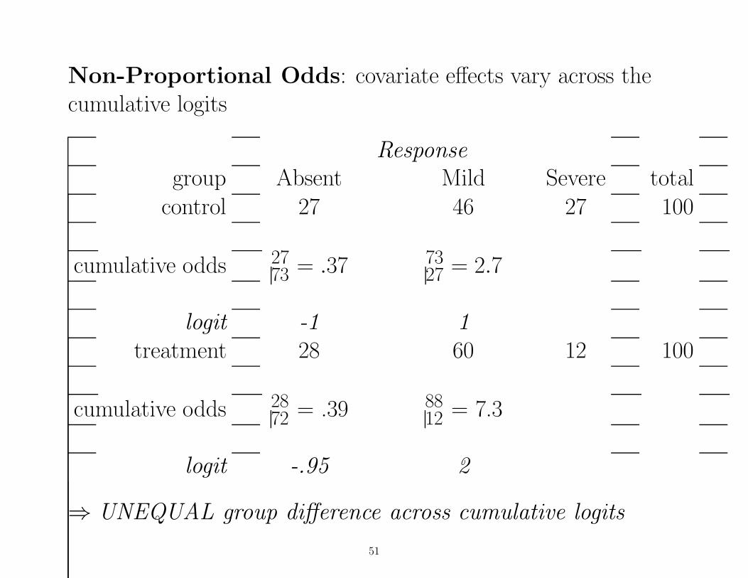
Non-Proportional Odds: covariate effects vary across thecumulative logits
Responsegroup Absent Mild Severe total
control 27 46 27 100
cumulative odds 2773 = .37 73
27 = 2.7
logit -1 1treatment 28 60 12 100
cumulative odds 2872 = .39 88
12 = 7.3
logit -.95 2
⇒ UNEQUAL group difference across cumulative logits
51
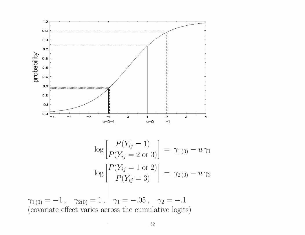
log
P (Yij = 1)
P (Yij = 2 or 3)
= γ1 (0) − u γ1
log
P (Yij = 1 or 2)
P (Yij = 3)
= γ2 (0) − u γ2
γ1 (0) = −1 , γ2(0) = 1 , γ1 = −.05 , γ2 = −.1(covariate effect varies across the cumulative logits)
52
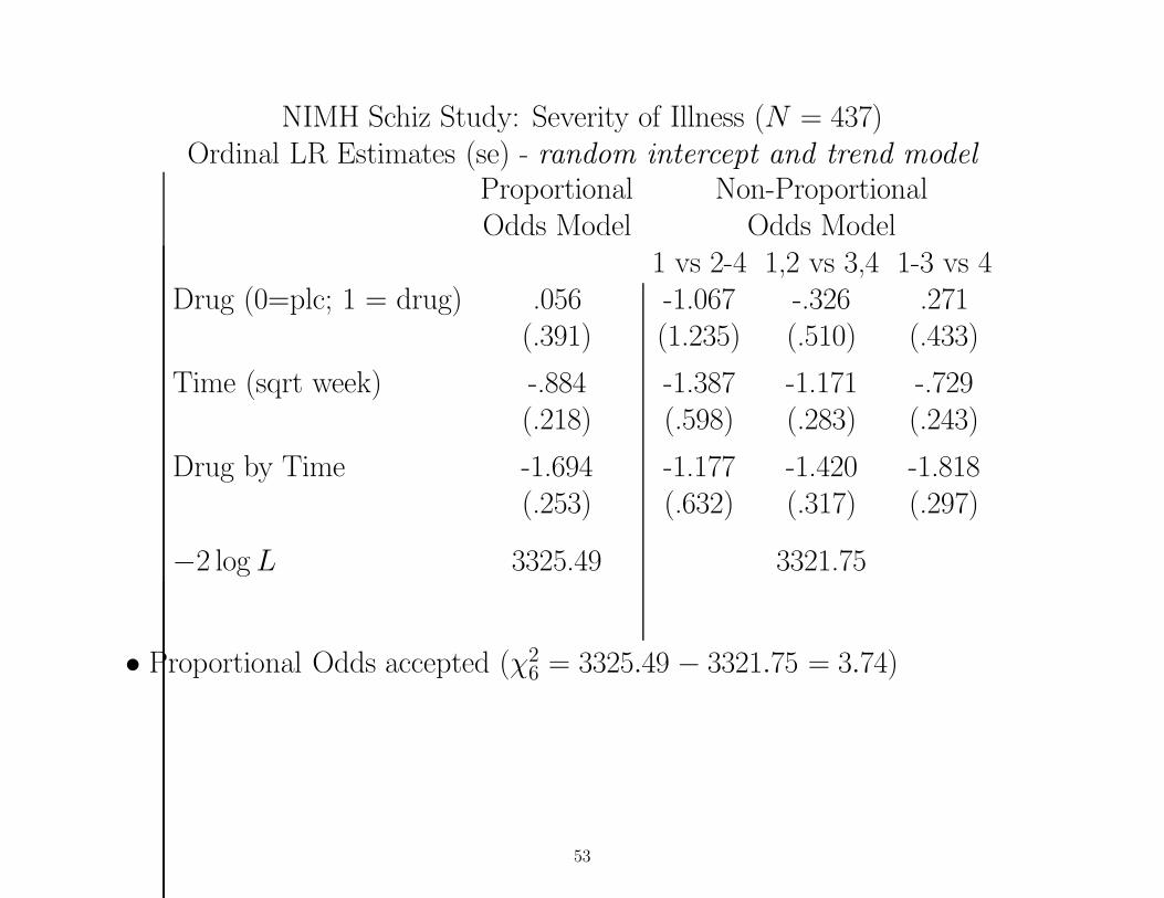
NIMH Schiz Study: Severity of Illness (N = 437)Ordinal LR Estimates (se) - random intercept and trend model
Proportional Non-ProportionalOdds Model Odds Model
1 vs 2-4 1,2 vs 3,4 1-3 vs 4Drug (0=plc; 1 = drug) .056 -1.067 -.326 .271
(.391) (1.235) (.510) (.433)
Time (sqrt week) -.884 -1.387 -1.171 -.729(.218) (.598) (.283) (.243)
Drug by Time -1.694 -1.177 -1.420 -1.818(.253) (.632) (.317) (.297)
−2 log L 3325.49 3321.75
• Proportional Odds accepted (χ26 = 3325.49 − 3321.75 = 3.74)
53

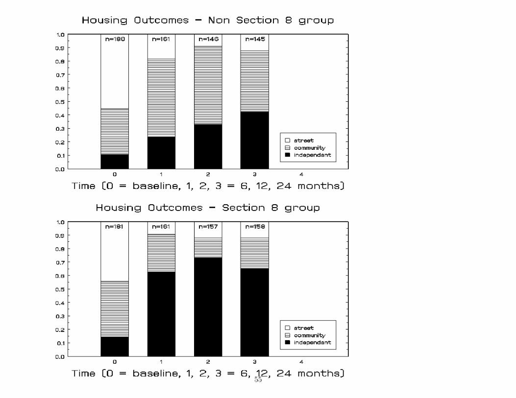
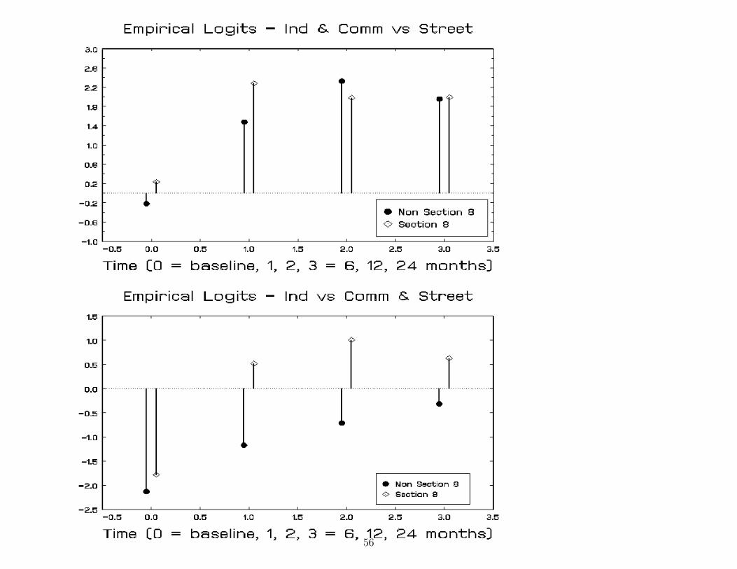
San Diego Homeless Research Project (Hough)
• 361 mentally ill subjects who were
– homeless or
– at very high risk of becoming homeless
• 2 conditions: HUD Section 8 rental certificates (yes/no)
• baseline and 6, 12, and 24 month follow-ups
• Categorical outcome: housing status
– streets / shelters (Y = 1)
– community / institutions (Y = 2)
– independent (Y = 3)
Question: Do Section 8 certificates influence housing statusacross time?
54
55
56
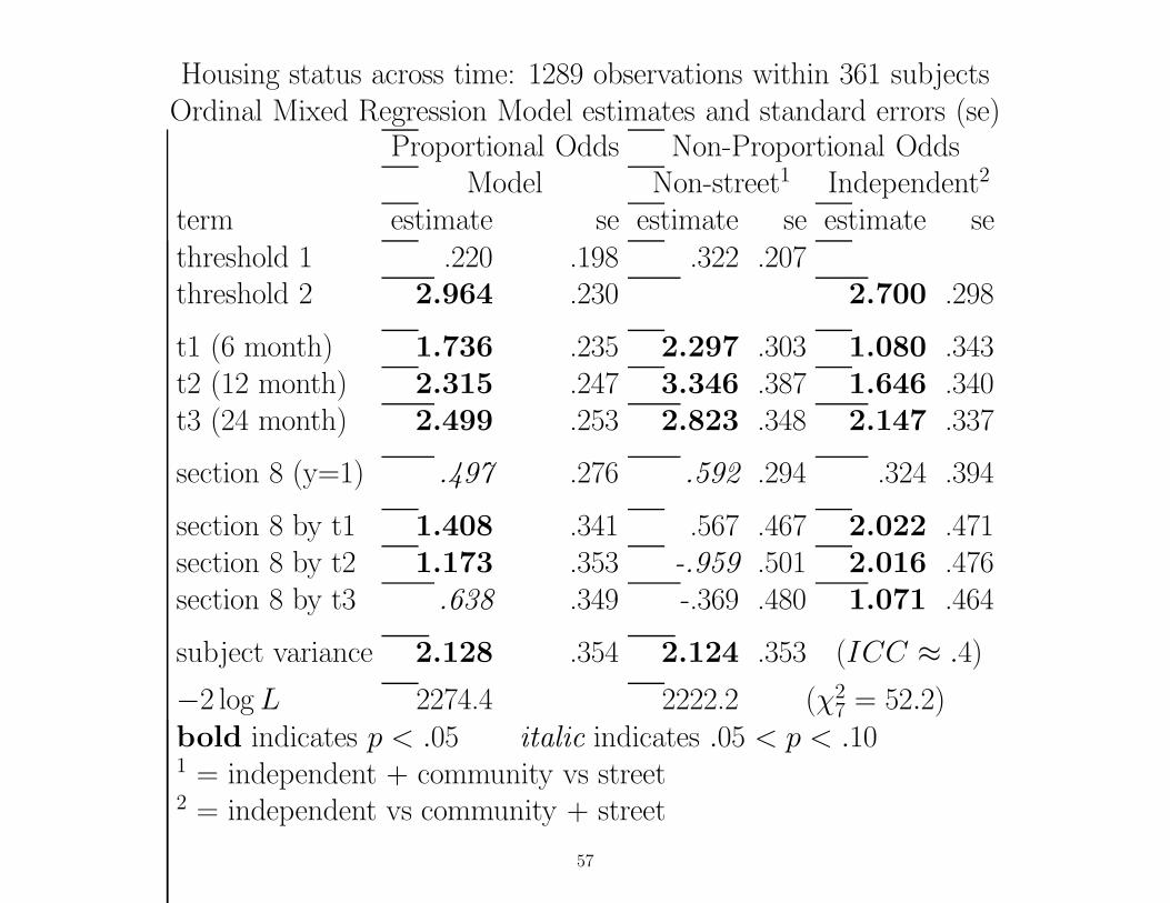
Housing status across time: 1289 observations within 361 subjectsOrdinal Mixed Regression Model estimates and standard errors (se)
Proportional Odds Non-Proportional OddsModel Non-street1 Independent2
term estimate se estimate se estimate sethreshold 1 .220 .198 .322 .207threshold 2 2.964 .230 2.700 .298
t1 (6 month) 1.736 .235 2.297 .303 1.080 .343t2 (12 month) 2.315 .247 3.346 .387 1.646 .340t3 (24 month) 2.499 .253 2.823 .348 2.147 .337
section 8 (y=1) .497 .276 .592 .294 .324 .394
section 8 by t1 1.408 .341 .567 .467 2.022 .471section 8 by t2 1.173 .353 -.959 .501 2.016 .476section 8 by t3 .638 .349 -.369 .480 1.071 .464
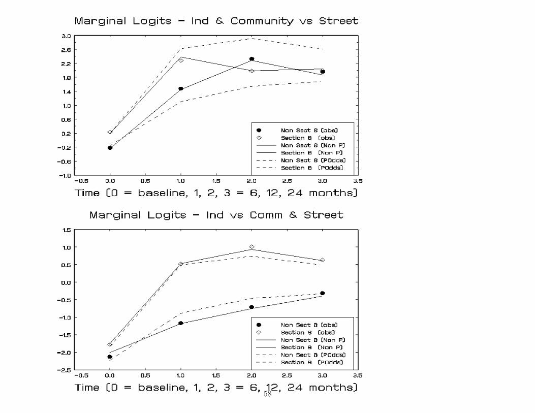
subject variance 2.128 .354 2.124 .353 (ICC ≈ .4)
−2 log L 2274.4 2222.2 (χ27 = 52.2)
bold indicates p < .05 italic indicates .05 < p < .101 = independent + community vs street2 = independent vs community + street
57
58
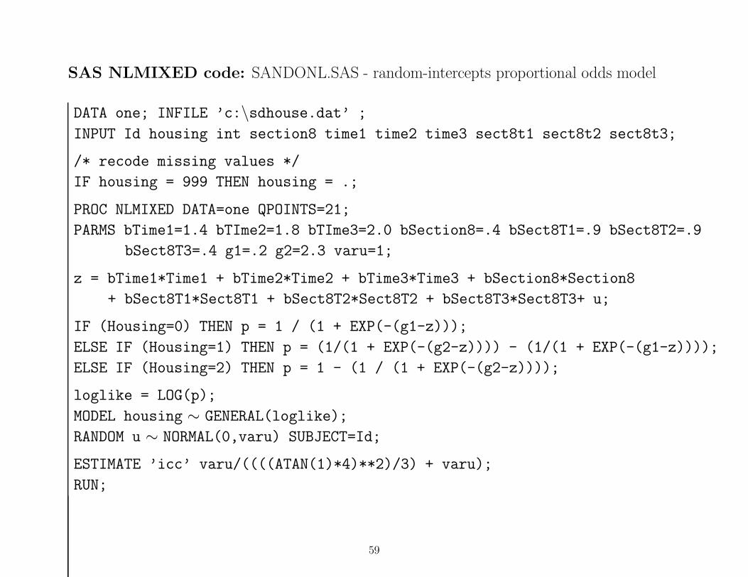
SAS NLMIXED code: SANDONL.SAS - random-intercepts proportional odds model
DATA one; INFILE ’c:\sdhouse.dat’ ;
INPUT Id housing int section8 time1 time2 time3 sect8t1 sect8t2 sect8t3;
/* recode missing values */
IF housing = 999 THEN housing = .;
PROC NLMIXED DATA=one QPOINTS=21;
PARMS bTime1=1.4 bTIme2=1.8 bTIme3=2.0 bSection8=.4 bSect8T1=.9 bSect8T2=.9
bSect8T3=.4 g1=.2 g2=2.3 varu=1;
z = bTime1*Time1 + bTime2*Time2 + bTime3*Time3 + bSection8*Section8
+ bSect8T1*Sect8T1 + bSect8T2*Sect8T2 + bSect8T3*Sect8T3+ u;
IF (Housing=0) THEN p = 1 / (1 + EXP(-(g1-z)));
ELSE IF (Housing=1) THEN p = (1/(1 + EXP(-(g2-z)))) - (1/(1 + EXP(-(g1-z))));
ELSE IF (Housing=2) THEN p = 1 - (1 / (1 + EXP(-(g2-z))));
loglike = LOG(p);
MODEL housing ∼ GENERAL(loglike);
RANDOM u ∼ NORMAL(0,varu) SUBJECT=Id;
ESTIMATE ’icc’ varu/((((ATAN(1)*4)**2)/3) + varu);
RUN;
59
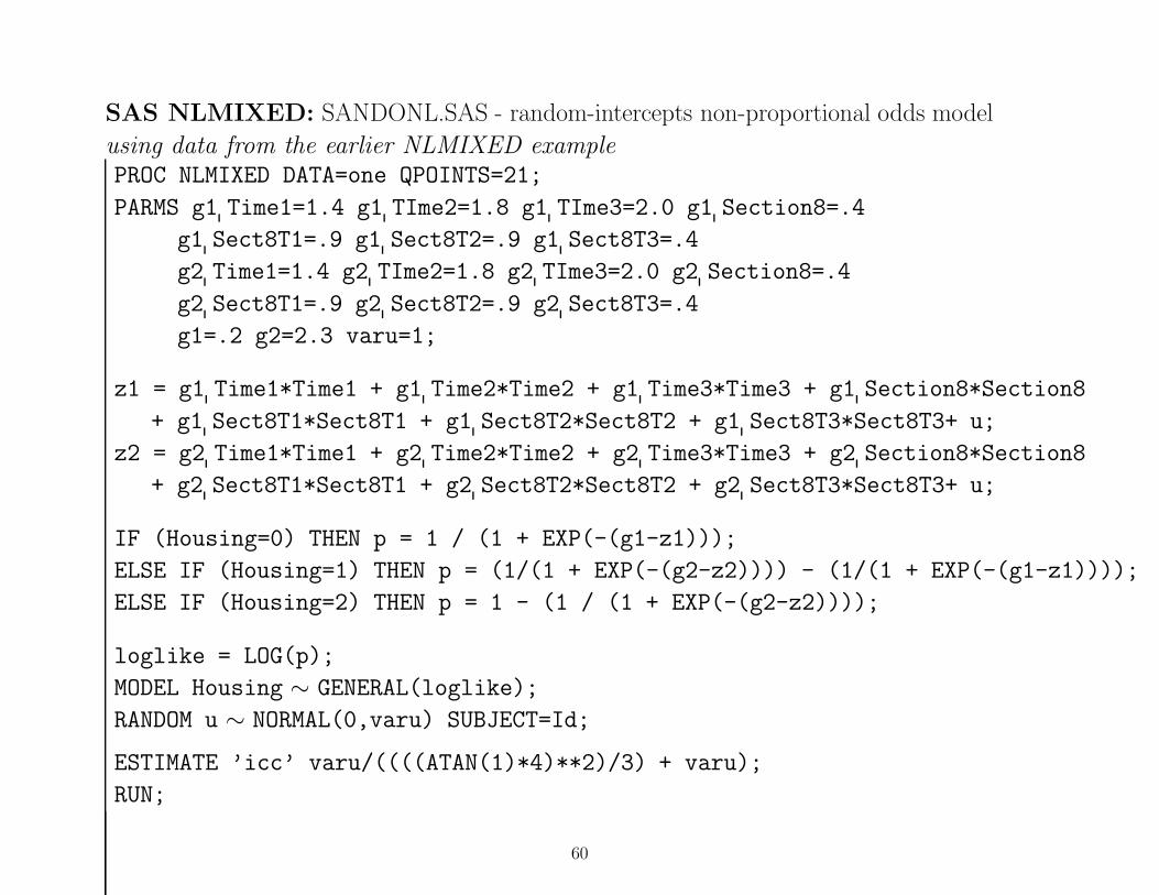
SAS NLMIXED: SANDONL.SAS - random-intercepts non-proportional odds model
using data from the earlier NLMIXED examplePROC NLMIXED DATA=one QPOINTS=21;
PARMS g1 Time1=1.4 g1 TIme2=1.8 g1 TIme3=2.0 g1 Section8=.4
g1 Sect8T1=.9 g1 Sect8T2=.9 g1 Sect8T3=.4
g2 Time1=1.4 g2 TIme2=1.8 g2 TIme3=2.0 g2 Section8=.4
g2 Sect8T1=.9 g2 Sect8T2=.9 g2 Sect8T3=.4
g1=.2 g2=2.3 varu=1;
z1 = g1 Time1*Time1 + g1 Time2*Time2 + g1 Time3*Time3 + g1 Section8*Section8
+ g1 Sect8T1*Sect8T1 + g1 Sect8T2*Sect8T2 + g1 Sect8T3*Sect8T3+ u;
z2 = g2 Time1*Time1 + g2 Time2*Time2 + g2 Time3*Time3 + g2 Section8*Section8
+ g2 Sect8T1*Sect8T1 + g2 Sect8T2*Sect8T2 + g2 Sect8T3*Sect8T3+ u;
IF (Housing=0) THEN p = 1 / (1 + EXP(-(g1-z1)));
ELSE IF (Housing=1) THEN p = (1/(1 + EXP(-(g2-z2)))) - (1/(1 + EXP(-(g1-z1))));
ELSE IF (Housing=2) THEN p = 1 - (1 / (1 + EXP(-(g2-z2))));
loglike = LOG(p);
MODEL Housing ∼ GENERAL(loglike);
RANDOM u ∼ NORMAL(0,varu) SUBJECT=Id;
ESTIMATE ’icc’ varu/((((ATAN(1)*4)**2)/3) + varu);
RUN;
60
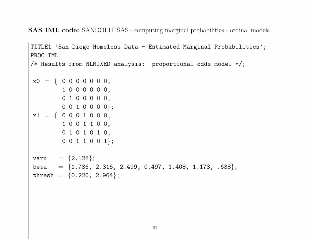
SAS IML code: SANDOFIT.SAS - computing marginal probabilities - ordinal models
TITLE1 ’San Diego Homeless Data - Estimated Marginal Probabilities’;
PROC IML;
/* Results from NLMIXED analysis: proportional odds model */;
x0 = { 0 0 0 0 0 0 0,
1 0 0 0 0 0 0,
0 1 0 0 0 0 0,
0 0 1 0 0 0 0};x1 = { 0 0 0 1 0 0 0,
1 0 0 1 1 0 0,
0 1 0 1 0 1 0,
0 0 1 1 0 0 1};
varu = {2.128};beta = {1.736, 2.315, 2.499, 0.497, 1.408, 1.173, .638};thresh = {0.220, 2.964};
61
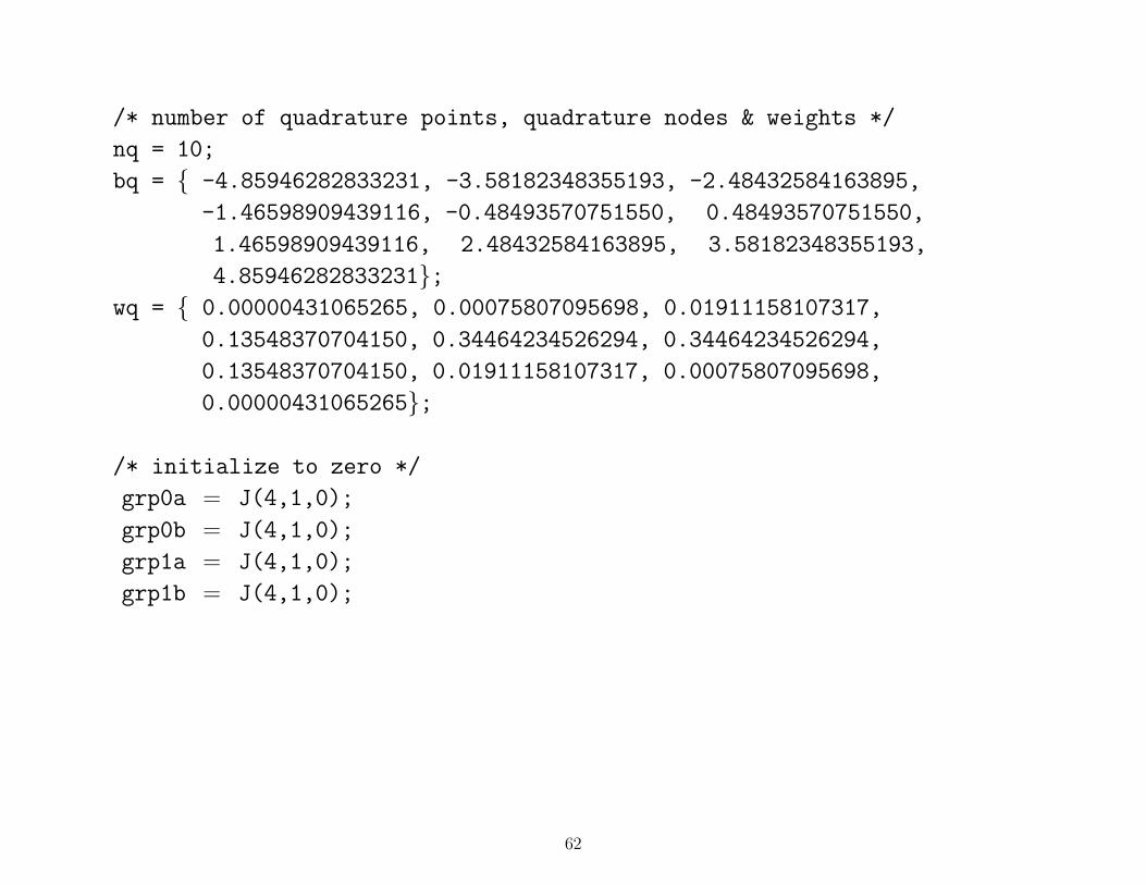
/* number of quadrature points, quadrature nodes & weights */
nq = 10;
bq = { -4.85946282833231, -3.58182348355193, -2.48432584163895,
-1.46598909439116, -0.48493570751550, 0.48493570751550,
1.46598909439116, 2.48432584163895, 3.58182348355193,
4.85946282833231};wq = { 0.00000431065265, 0.00075807095698, 0.01911158107317,
0.13548370704150, 0.34464234526294, 0.34464234526294,
0.13548370704150, 0.01911158107317, 0.00075807095698,
0.00000431065265};
/* initialize to zero */
grp0a = J(4,1,0);
grp0b = J(4,1,0);
grp1a = J(4,1,0);
grp1b = J(4,1,0);
62
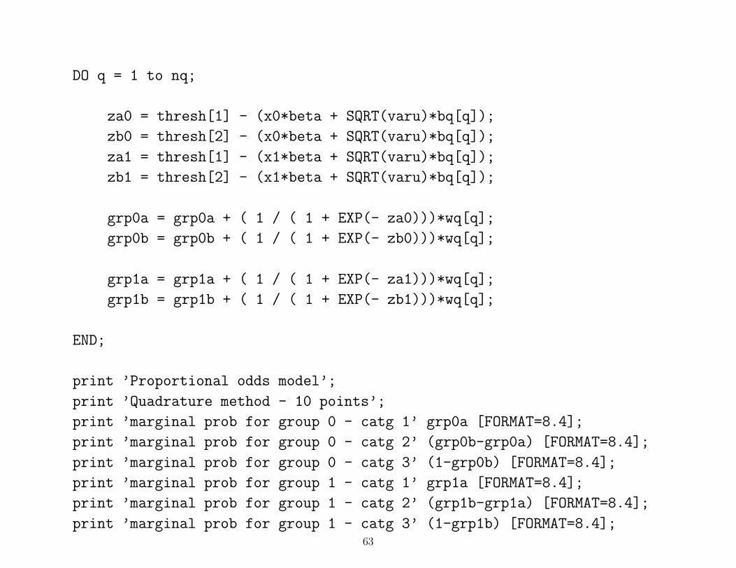
DO q = 1 to nq;
za0 = thresh[1] - (x0*beta + SQRT(varu)*bq[q]);
zb0 = thresh[2] - (x0*beta + SQRT(varu)*bq[q]);
za1 = thresh[1] - (x1*beta + SQRT(varu)*bq[q]);
zb1 = thresh[2] - (x1*beta + SQRT(varu)*bq[q]);
grp0a = grp0a + ( 1 / ( 1 + EXP(- za0)))*wq[q];
grp0b = grp0b + ( 1 / ( 1 + EXP(- zb0)))*wq[q];
grp1a = grp1a + ( 1 / ( 1 + EXP(- za1)))*wq[q];
grp1b = grp1b + ( 1 / ( 1 + EXP(- zb1)))*wq[q];
END;
print ’Proportional odds model’;
print ’Quadrature method - 10 points’;
print ’marginal prob for group 0 - catg 1’ grp0a [FORMAT=8.4];
print ’marginal prob for group 0 - catg 2’ (grp0b-grp0a) [FORMAT=8.4];
print ’marginal prob for group 0 - catg 3’ (1-grp0b) [FORMAT=8.4];
print ’marginal prob for group 1 - catg 1’ grp1a [FORMAT=8.4];
print ’marginal prob for group 1 - catg 2’ (grp1b-grp1a) [FORMAT=8.4];
print ’marginal prob for group 1 - catg 3’ (1-grp1b) [FORMAT=8.4];63
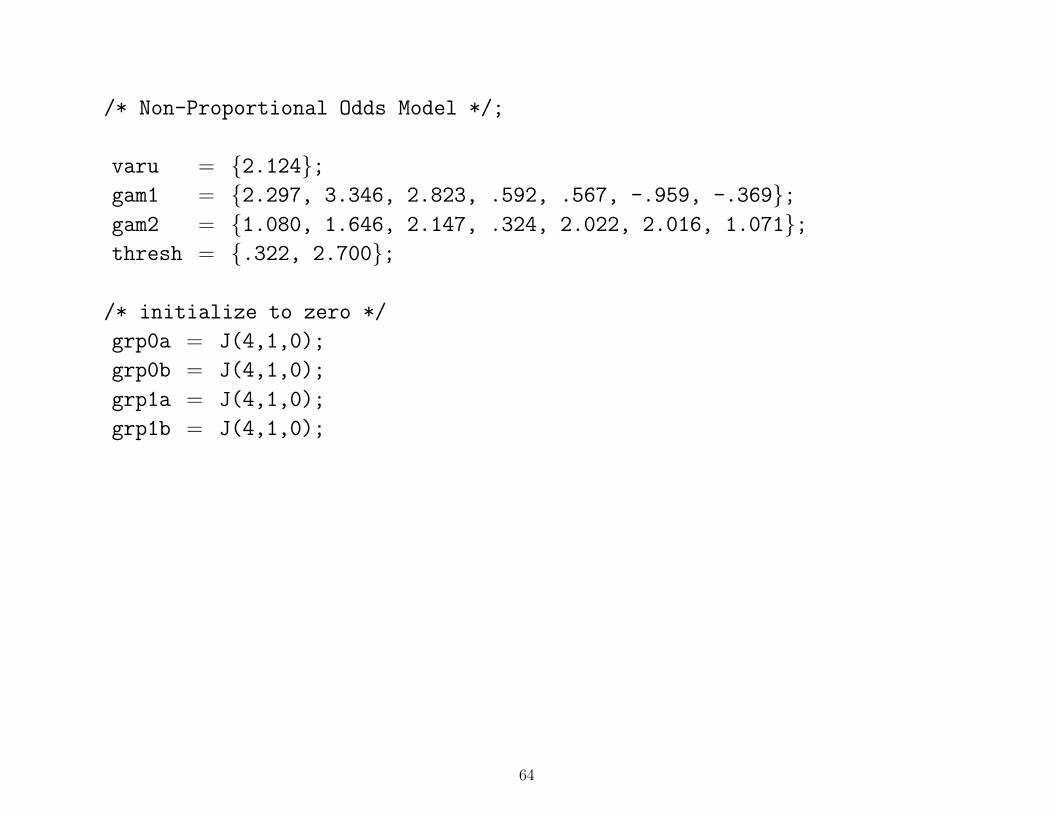
/* Non-Proportional Odds Model */;
varu = {2.124};gam1 = {2.297, 3.346, 2.823, .592, .567, -.959, -.369};gam2 = {1.080, 1.646, 2.147, .324, 2.022, 2.016, 1.071};thresh = {.322, 2.700};
/* initialize to zero */
grp0a = J(4,1,0);
grp0b = J(4,1,0);
grp1a = J(4,1,0);
grp1b = J(4,1,0);
64
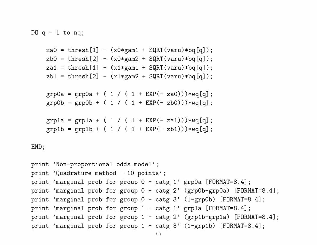
DO q = 1 to nq;
za0 = thresh[1] - (x0*gam1 + SQRT(varu)*bq[q]);
zb0 = thresh[2] - (x0*gam2 + SQRT(varu)*bq[q]);
za1 = thresh[1] - (x1*gam1 + SQRT(varu)*bq[q]);
zb1 = thresh[2] - (x1*gam2 + SQRT(varu)*bq[q]);
grp0a = grp0a + ( 1 / ( 1 + EXP(- za0)))*wq[q];
grp0b = grp0b + ( 1 / ( 1 + EXP(- zb0)))*wq[q];
grp1a = grp1a + ( 1 / ( 1 + EXP(- za1)))*wq[q];
grp1b = grp1b + ( 1 / ( 1 + EXP(- zb1)))*wq[q];
END;
print ’Non-proportional odds model’;
print ’Quadrature method - 10 points’;
print ’marginal prob for group 0 - catg 1’ grp0a [FORMAT=8.4];
print ’marginal prob for group 0 - catg 2’ (grp0b-grp0a) [FORMAT=8.4];
print ’marginal prob for group 0 - catg 3’ (1-grp0b) [FORMAT=8.4];
print ’marginal prob for group 1 - catg 1’ grp1a [FORMAT=8.4];
print ’marginal prob for group 1 - catg 2’ (grp1b-grp1a) [FORMAT=8.4];
print ’marginal prob for group 1 - catg 3’ (1-grp1b) [FORMAT=8.4];65
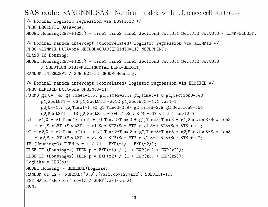
Mixed-effects Multinomial Logistic RegressionModel for Nominal Responses (Hedeker, 2003)
Yij = nominal response of level-2 unit i and level-1 unit j
logpijc
pij1= u′
ijγc + z′ijυic c = 2, 3, . . . C
• C − 1 contrasts to reference cell (c = 1)
• regression effects γc vary across contrasts
• (C − 1) × r random-effects ∼ N(0,Συ)
For example, with C = 3
contrast ordinal nominalc1 2 & 3 vs 1 2 vs 1c2 3 vs 1 & 2 3 vs 1
66

Model in terms of the category probabilities
pijc = Pr(Yij = c | υic) =exp(zijc)
1 + ∑Ch=2 exp(zijh)
for c = 2, 3, . . . , C
pij1 = Pr(Yij = 1 | υic) =1
1 + ∑Ch=2 exp(zijh)
where the multinomial logit zijc = u′ijγc + z′ijυic
67
68
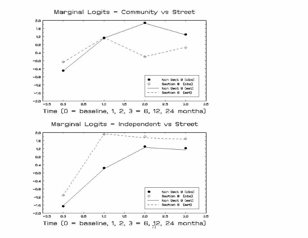
Housing status across time: 1289 observations within 361 subjectsNominal Mixed Regression Model estimates & standard errors (se)
Community vs Street Independent vs Streetterm estimate se estimate seintercept -.635 .198 -2.600 .353
t1 (6 month) 1.914 .299 2.332 .410t2 (12 month) 2.686 .373 3.677 .468t3 (24 month) 1.982 .342 3.735 .444
section 8 (y=1) .518 .276 .675 .445
section 8 by t1 -.639 .469 1.886 .591section 8 by t2 -2.499 .534 .556 .617section 8 by t3 -1.234 .491 .256 .589
subject variance 1.099 .325 3.249 .674
−2 log L 2214.35
bold indicates p < .05 italic indicates .05 < p < .10
69
Housing status across time: 1289 observations within 361 subjectsNominal Mixed Regression Model estimates & standard errors (se)
Community vs Street Independent vs Streetterm estimate se estimate seintercept -.622 .233 -2.600 .384
t1 (6 month) 2.374 .348 2.888 .454t2 (12 month) 3.345 .442 4.394 .530t3 (24 month) 2.589 .402 4.310 .496
section 8 (y=1) .652 .328 .831 .494
section 8 by t1 -.331 .523 1.969 .644section 8 by t2 -2.475 .590 .287 .677section 8 by t3 -1.160 .544 .202 .644
subject variance 2.702 .325 5.821 1.136covariance 2.884 .765 r = .73
−2 log L 2180.9 χ21 = 33.5
bold indicates p < .05 italic indicates .05 < p < .10
70
71
72
SAS code: SANDNNL.SAS - Nominal models with reference cell contrasts/* Nominal logistic regression via LOGISTIC */
PROC LOGISTIC DATA=one;
MODEL Housing(REF=FIRST) = Time1 Time2 Time3 Section8 Sect8T1 Sect8T2 Sect8T3 / LINK=GLOGIT;
/* Nominal random intercept (uncorrelated) logistic regression via GLIMMIX */
PROC GLIMMIX DATA=one METHOD=QUAD(QPOINTS=11) NOCLPRINT;
CLASS Id Housing;
MODEL Housing(REF=FIRST) = Time1 Time2 Time3 Section8 Sect8T1 Sect8T2 Sect8T3
/ SOLUTION DIST=MULTINOMIAL LINK=GLOGIT;
RANDOM INTERCEPT / SUBJECT=Id GROUP=Housing;
/* Nominal random intercept (correlated) logistic regression via NLMIXED */
PROC NLMIXED DATA=one QPOINTS=11;
PARMS g1 0=-.49 g1 Time1=1.63 g1 Time2=2.37 g1 Time3=1.8 g1 Section8=.43
g1 Sect8T1=-.46 g1 Sect8T2=-2.12 g1 Sect8T3=-1.1 var1=1
g2 0=-1.7 g2 Time1=1.90 g2 Time2=2.97 g2 Time3=2.9 g2 Section8=.54
g2 Sect8T1=1.13 g2 Sect8T2=-.04 g2 Sect8T3=-.07 var2=1 cov12=0;
z1 = g1 0 + g1 Time1*Time1 + g1 Time2*Time2 + g1 Time3*Time3 + g1 Section8*Section8
+ g1 Sect8T1*Sect8T1 + g1 Sect8T2*Sect8T2 + g1 Sect8T3*Sect8T3 + u1;
z2 = g2 0 + g2 Time1*Time1 + g2 Time2*Time2 + g2 Time3*Time3 + g2 Section8*Section8
+ g2 Sect8T1*Sect8T1 + g2 Sect8T2*Sect8T2 + g2 Sect8T3*Sect8T3 + u2;
IF (Housing=0) THEN p = 1 / (1 + EXP(z1) + EXP(z2));
ELSE IF (Housing=1) THEN p = EXP(z1) / (1 + EXP(z1) + EXP(z2));
ELSE IF (Housing=2) THEN p = EXP(z2) / (1 + EXP(z1) + EXP(z2));
LogLike = LOG(p);
MODEL Housing ∼ GENERAL(LogLike);
RANDOM u1 u2 ∼ NORMAL([0,0],[var1,cov12,var2]) SUBJECT=Id;
ESTIMATE ’RE corr’ cov12 / SQRT(var1*var2);
RUN;
73
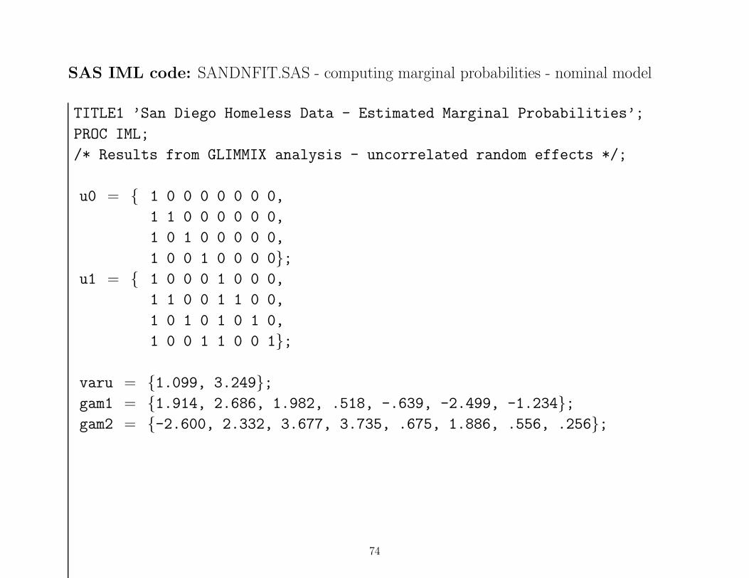
SAS IML code: SANDNFIT.SAS - computing marginal probabilities - nominal model
TITLE1 ’San Diego Homeless Data - Estimated Marginal Probabilities’;
PROC IML;
/* Results from GLIMMIX analysis - uncorrelated random effects */;
u0 = { 1 0 0 0 0 0 0 0,
1 1 0 0 0 0 0 0,
1 0 1 0 0 0 0 0,
1 0 0 1 0 0 0 0};u1 = { 1 0 0 0 1 0 0 0,
1 1 0 0 1 1 0 0,
1 0 1 0 1 0 1 0,
1 0 0 1 1 0 0 1};
varu = {1.099, 3.249};gam1 = {1.914, 2.686, 1.982, .518, -.639, -2.499, -1.234};gam2 = {-2.600, 2.332, 3.677, 3.735, .675, 1.886, .556, .256};
74
/* number of quadrature points, quadrature nodes & weights */
nq = 10;
bq = { -4.85946282833231, -3.58182348355193, -2.48432584163895,
-1.46598909439116, -0.48493570751550, 0.48493570751550,
1.46598909439116, 2.48432584163895, 3.58182348355193,
4.85946282833231};wq = { 0.00000431065265, 0.00075807095698, 0.01911158107317,
0.13548370704150, 0.34464234526294, 0.34464234526294,
0.13548370704150, 0.01911158107317, 0.00075807095698,
0.00000431065265};
/* initialize to zero */
grp0a = J(4,1,0); grp0b = J(4,1,0); grp0c = J(4,1,0);
grp1a = J(4,1,0); grp1b = J(4,1,0); grp1c = J(4,1,0);
75
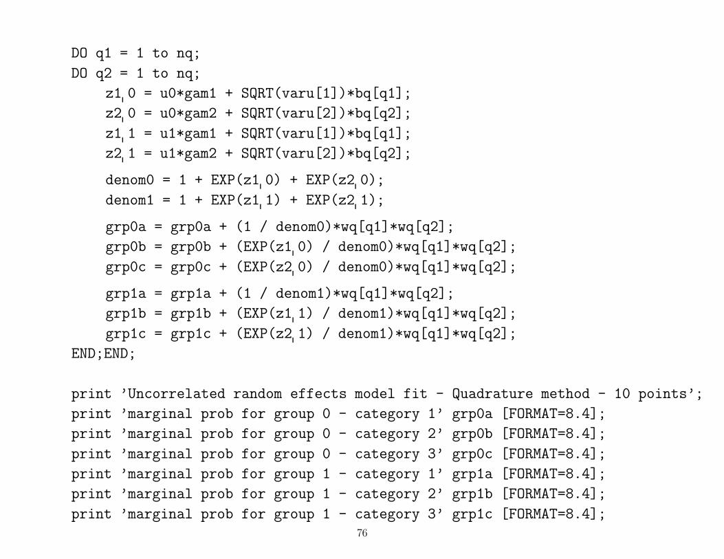
DO q1 = 1 to nq;
DO q2 = 1 to nq;
z1 0 = u0*gam1 + SQRT(varu[1])*bq[q1];
z2 0 = u0*gam2 + SQRT(varu[2])*bq[q2];
z1 1 = u1*gam1 + SQRT(varu[1])*bq[q1];
z2 1 = u1*gam2 + SQRT(varu[2])*bq[q2];
denom0 = 1 + EXP(z1 0) + EXP(z2 0);
denom1 = 1 + EXP(z1 1) + EXP(z2 1);
grp0a = grp0a + (1 / denom0)*wq[q1]*wq[q2];
grp0b = grp0b + (EXP(z1 0) / denom0)*wq[q1]*wq[q2];
grp0c = grp0c + (EXP(z2 0) / denom0)*wq[q1]*wq[q2];
grp1a = grp1a + (1 / denom1)*wq[q1]*wq[q2];
grp1b = grp1b + (EXP(z1 1) / denom1)*wq[q1]*wq[q2];
grp1c = grp1c + (EXP(z2 1) / denom1)*wq[q1]*wq[q2];
END;END;
print ’Uncorrelated random effects model fit - Quadrature method - 10 points’;
print ’marginal prob for group 0 - category 1’ grp0a [FORMAT=8.4];
print ’marginal prob for group 0 - category 2’ grp0b [FORMAT=8.4];
print ’marginal prob for group 0 - category 3’ grp0c [FORMAT=8.4];
print ’marginal prob for group 1 - category 1’ grp1a [FORMAT=8.4];
print ’marginal prob for group 1 - category 2’ grp1b [FORMAT=8.4];
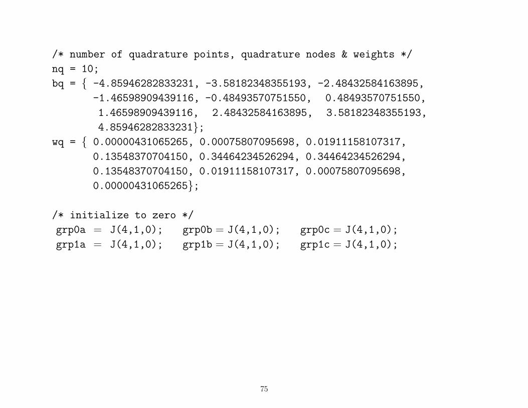
print ’marginal prob for group 1 - category 3’ grp1c [FORMAT=8.4];76
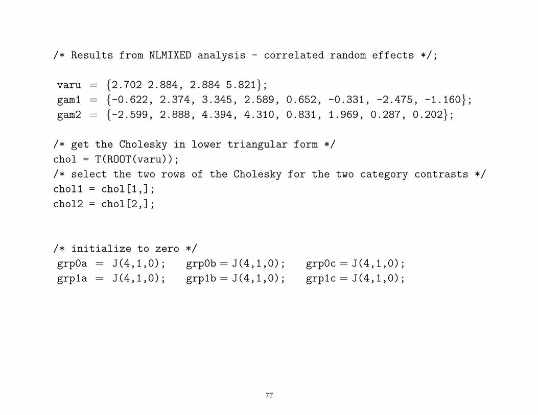
/* Results from NLMIXED analysis - correlated random effects */;
varu = {2.702 2.884, 2.884 5.821};gam1 = {-0.622, 2.374, 3.345, 2.589, 0.652, -0.331, -2.475, -1.160};gam2 = {-2.599, 2.888, 4.394, 4.310, 0.831, 1.969, 0.287, 0.202};
/* get the Cholesky in lower triangular form */
chol = T(ROOT(varu));
/* select the two rows of the Cholesky for the two category contrasts */
chol1 = chol[1,];
chol2 = chol[2,];
/* initialize to zero */
grp0a = J(4,1,0); grp0b = J(4,1,0); grp0c = J(4,1,0);
grp1a = J(4,1,0); grp1b = J(4,1,0); grp1c = J(4,1,0);
77
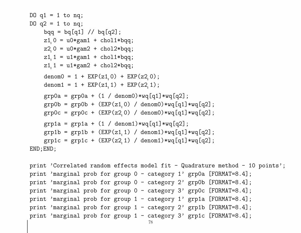
DO q1 = 1 to nq;
DO q2 = 1 to nq;
bqq = bq[q1] // bq[q2];
z1 0 = u0*gam1 + chol1*bqq;
z2 0 = u0*gam2 + chol2*bqq;
z1 1 = u1*gam1 + chol1*bqq;
z1 1 = u1*gam2 + chol2*bqq;
denom0 = 1 + EXP(z1 0) + EXP(z2 0);
denom1 = 1 + EXP(z1 1) + EXP(z2 1);
grp0a = grp0a + (1 / denom0)*wq[q1]*wq[q2];
grp0b = grp0b + (EXP(z1 0) / denom0)*wq[q1]*wq[q2];
grp0c = grp0c + (EXP(z2 0) / denom0)*wq[q1]*wq[q2];
grp1a = grp1a + (1 / denom1)*wq[q1]*wq[q2];
grp1b = grp1b + (EXP(z1 1) / denom1)*wq[q1]*wq[q2];
grp1c = grp1c + (EXP(z2 1) / denom1)*wq[q1]*wq[q2];
END;END;
print ’Correlated random effects model fit - Quadrature method - 10 points’;
print ’marginal prob for group 0 - category 1’ grp0a [FORMAT=8.4];
print ’marginal prob for group 0 - category 2’ grp0b [FORMAT=8.4];
print ’marginal prob for group 0 - category 3’ grp0c [FORMAT=8.4];
print ’marginal prob for group 1 - category 1’ grp1a [FORMAT=8.4];
print ’marginal prob for group 1 - category 2’ grp1b [FORMAT=8.4];
print ’marginal prob for group 1 - category 3’ grp1c [FORMAT=8.4];78
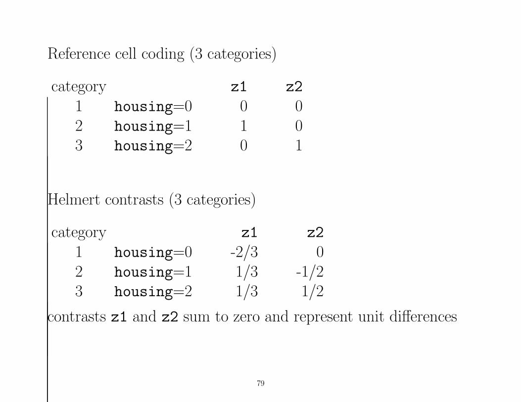
Reference cell coding (3 categories)
category z1 z2
1 housing=0 0 02 housing=1 1 03 housing=2 0 1
Helmert contrasts (3 categories)
category z1 z2
1 housing=0 -2/3 02 housing=1 1/3 -1/23 housing=2 1/3 1/2
contrasts z1 and z2 sum to zero and represent unit differences
79
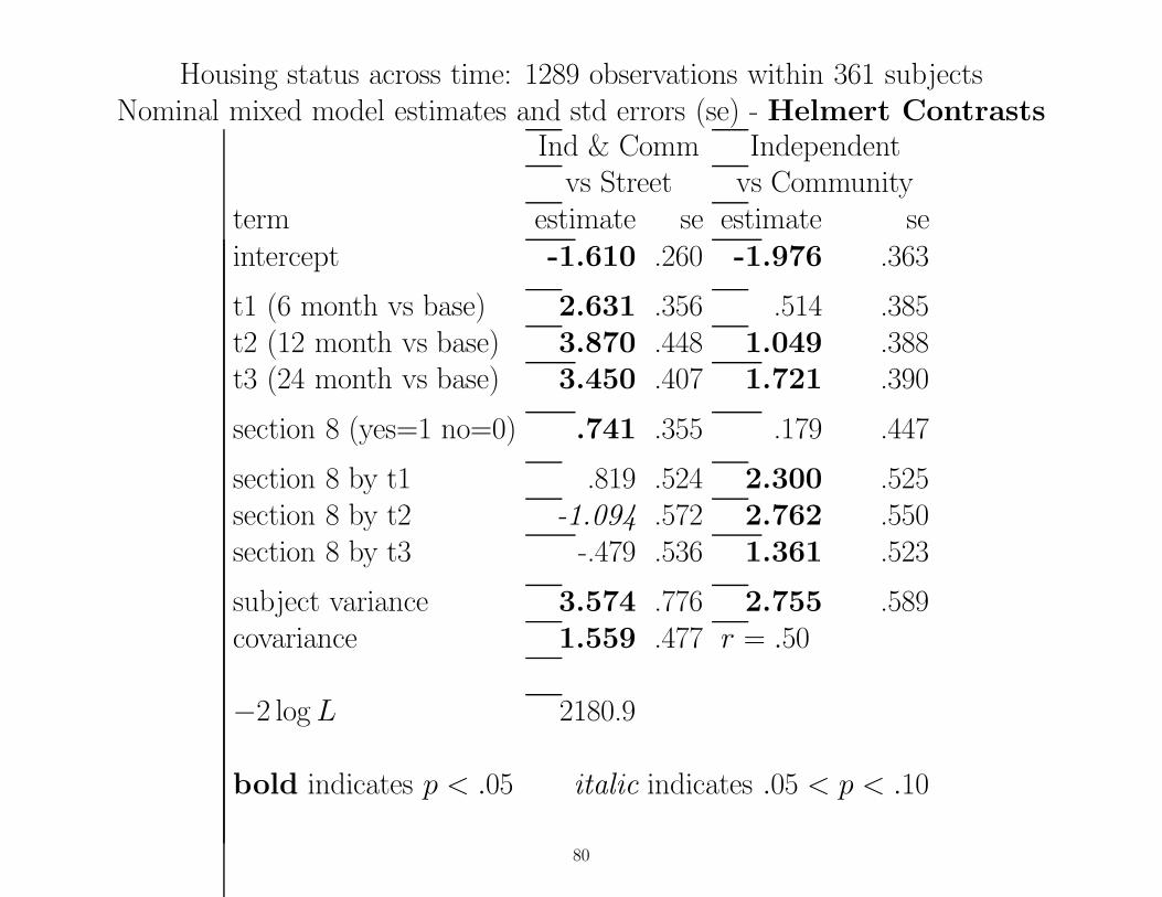
Housing status across time: 1289 observations within 361 subjectsNominal mixed model estimates and std errors (se) - Helmert Contrasts
Ind & Comm Independentvs Street vs Community
term estimate se estimate seintercept -1.610 .260 -1.976 .363
t1 (6 month vs base) 2.631 .356 .514 .385t2 (12 month vs base) 3.870 .448 1.049 .388t3 (24 month vs base) 3.450 .407 1.721 .390
section 8 (yes=1 no=0) .741 .355 .179 .447
section 8 by t1 .819 .524 2.300 .525section 8 by t2 -1.094 .572 2.762 .550section 8 by t3 -.479 .536 1.361 .523
subject variance 3.574 .776 2.755 .589covariance 1.559 .477 r = .50
−2 log L 2180.9
bold indicates p < .05 italic indicates .05 < p < .10
80
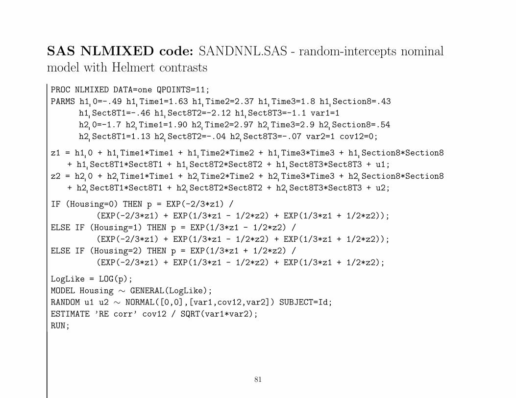
SAS NLMIXED code: SANDNNL.SAS - random-intercepts nominalmodel with Helmert contrasts
PROC NLMIXED DATA=one QPOINTS=11;
PARMS h1 0=-.49 h1 Time1=1.63 h1 Time2=2.37 h1 Time3=1.8 h1 Section8=.43
h1 Sect8T1=-.46 h1 Sect8T2=-2.12 h1 Sect8T3=-1.1 var1=1
h2 0=-1.7 h2 Time1=1.90 h2 Time2=2.97 h2 Time3=2.9 h2 Section8=.54
h2 Sect8T1=1.13 h2 Sect8T2=-.04 h2 Sect8T3=-.07 var2=1 cov12=0;
z1 = h1 0 + h1 Time1*Time1 + h1 Time2*Time2 + h1 Time3*Time3 + h1 Section8*Section8
+ h1 Sect8T1*Sect8T1 + h1 Sect8T2*Sect8T2 + h1 Sect8T3*Sect8T3 + u1;
z2 = h2 0 + h2 Time1*Time1 + h2 Time2*Time2 + h2 Time3*Time3 + h2 Section8*Section8
+ h2 Sect8T1*Sect8T1 + h2 Sect8T2*Sect8T2 + h2 Sect8T3*Sect8T3 + u2;
IF (Housing=0) THEN p = EXP(-2/3*z1) /
(EXP(-2/3*z1) + EXP(1/3*z1 - 1/2*z2) + EXP(1/3*z1 + 1/2*z2));
ELSE IF (Housing=1) THEN p = EXP(1/3*z1 - 1/2*z2) /
(EXP(-2/3*z1) + EXP(1/3*z1 - 1/2*z2) + EXP(1/3*z1 + 1/2*z2));
ELSE IF (Housing=2) THEN p = EXP(1/3*z1 + 1/2*z2) /
(EXP(-2/3*z1) + EXP(1/3*z1 - 1/2*z2) + EXP(1/3*z1 + 1/2*z2);
LogLike = LOG(p);
MODEL Housing ∼ GENERAL(LogLike);
RANDOM u1 u2 ∼ NORMAL([0,0],[var1,cov12,var2]) SUBJECT=Id;
ESTIMATE ’RE corr’ cov12 / SQRT(var1*var2);
RUN;
81

Summary
Models for longitudinal categorical data as developed as modelsfor continuous data
• Proportional odds models
• Non and partial proportional odds models
• Nominal models (with Reference-cell or Helmert contrasts)
• Scaling models (Hedeker, Berbaum, & Mermelstein, 2006;Hedeker, Demirtas, & Mermelstein, 2009)
Available software includes SAS PROCs GLIMMIX &NLMIXED, STATA, SuperMix, MIXOR, MIXNO, ...
82

SuperMix
• Free student and 15-day trial editionshttp://www.ssicentral.com/supermix/downloads.html
• Datasets and exampleshttp://www.ssicentral.com/supermix/examples.html
• Manual and documentation in PDF formhttp://www.ssicentral.com/supermix/resources.html
83