Econ 2840: Growth Regressions

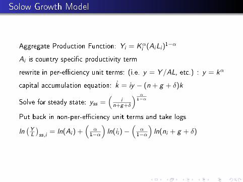
Solow Growth Model

Aggregate Production Function: Yi = Kαi (AiLi )

1−α

Ai is country speci�c productivity term

rewrite in per-e�ciency unit terms: (i.e. y = Y /AL, etc.) : y = kα

capital accumulation equation: k = iy − (n + g + δ)k

Solve for steady state: yss =(

in+g+δ

) α1−α

Put back in non-per-e�ciency unit terms and take logs

ln(YL

)ss,i

= ln(Ai ) +(

α1−α

)ln(ii ) −

(α

1−α

)ln(ni + g + δ)

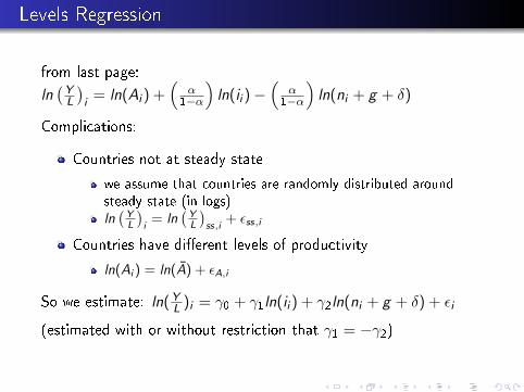
Levels Regression

from last page:

ln(YL

)i

= ln(Ai ) +(

α1−α

)ln(ii ) −

(α

1−α

)ln(ni + g + δ)

Complications:

Countries not at steady state

we assume that countries are randomly distributed aroundsteady state (in logs)ln(YL

)i

= ln(YL

)ss,i

+ εss,i

Countries have di�erent levels of productivity

ln(Ai ) = ln(A) + εA,i

So we estimate: ln(YL )i = γ0 + γ1ln(ii ) + γ2ln(ni + g + δ) + εi

(estimated with or without restriction that γ1 = −γ2)

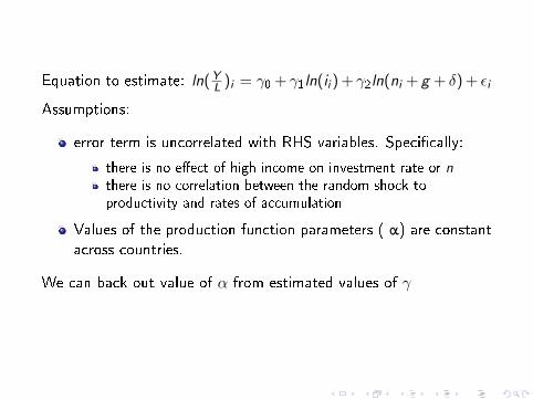
Equation to estimate: ln(YL )i = γ0 + γ1ln(ii ) + γ2ln(ni + g + δ) + εi

Assumptions:

error term is uncorrelated with RHS variables. Speci�cally:

there is no e�ect of high income on investment rate or nthere is no correlation between the random shock toproductivity and rates of accumulation

Values of the production function parameters ( α) are constantacross countries.

We can back out value of α from estimated values of γ

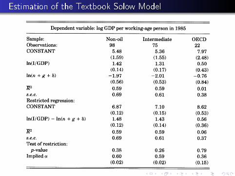
Estimation of the Textbook Solow Model

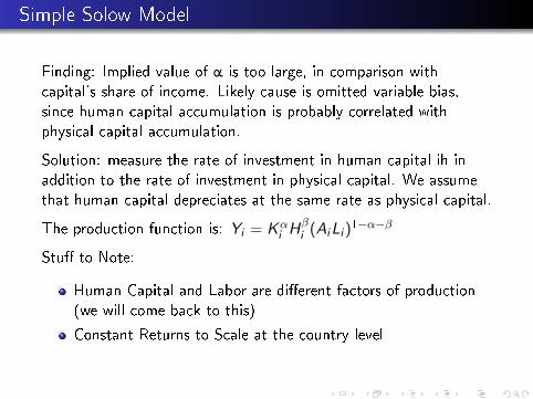
Simple Solow Model

Finding: Implied value of α is too large, in comparison withcapital's share of income. Likely cause is omitted variable bias,since human capital accumulation is probably correlated withphysical capital accumulation.

Solution: measure the rate of investment in human capital ih inaddition to the rate of investment in physical capital. We assumethat human capital depreciates at the same rate as physical capital.

The production function is: Yi = Kαi H

βi (AiLi )

1−α−β

Stu� to Note:

Human Capital and Labor are di�erent factors of production(we will come back to this)

Constant Returns to Scale at the country level

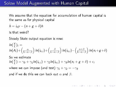
Solow Model Augmented with Human Capital

We assume that the equation for accumulation of human capital isthe same as for physical capital

h = ihy − (n + g + δ)h

Is that weird?

Steady State output equation is now:

ln(YL )i =

ln(Ai )+(

α1−α−β

)ln(ik,i )+

(β

1−α−β

)ln(ih,i )−

(α+β

1−α−β

)ln(ni+g+δ)

So we estimateln(YL ) = γ0 + γ1ln(ik,i ) + γ2ln(ih,i ) + γ3ln(ni + g + δ) + εi

where we can impose (and test) γ1 + γ2 = −γ3and if we do this we can back out α and β.

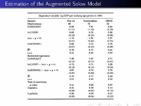
Estimation of the Augmented Solow Model

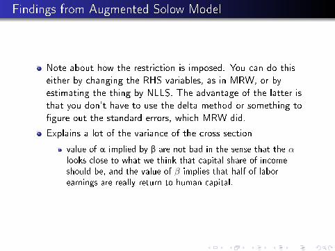
Findings from Augmented Solow Model

Note about how the restriction is imposed. You can do thiseither by changing the RHS variables, as in MRW, or byestimating the thing by NLLS. The advantage of the latter isthat you don't have to use the delta method or something to�gure out the standard errors, which MRW did.

Explains a lot of the variance of the cross section

value of α implied by β are not bad in the sense that the αlooks close to what we think that capital share of incomeshould be, and the value of β implies that half of laborearnings are really return to human capital.

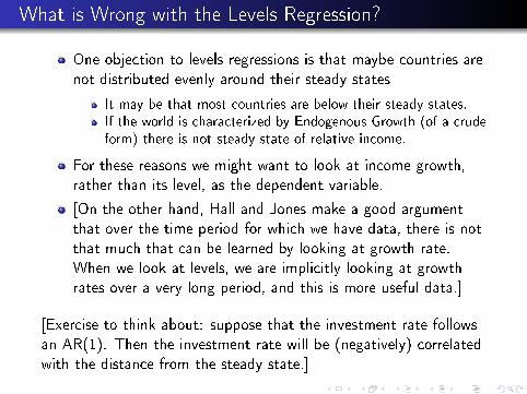
What is Wrong with the Levels Regression?

One objection to levels regressions is that maybe countries arenot distributed evenly around their steady states

It may be that most countries are below their steady states.If the world is characterized by Endogenous Growth (of a crudeform) there is not steady state of relative income.

For these reasons we might want to look at income growth,rather than its level, as the dependent variable.

[On the other hand, Hall and Jones make a good argumentthat over the time period for which we have data, there is notthat much that can be learned by looking at growth rate.When we look at levels, we are implicitly looking at growthrates over a very long period, and this is more useful data.]

[Exercise to think about: suppose that the investment rate followsan AR(1). Then the investment rate will be (negatively) correlatedwith the distance from the steady state.]

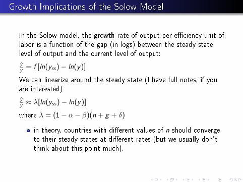
Growth Implications of the Solow Model

In the Solow model, the growth rate of output per e�ciency unit oflabor is a function of the gap (in logs) between the steady statelevel of output and the current level of output:

yy = f [ln(yss) − ln(y)]

We can linearize around the steady state (I have full notes, if youare interested)

yy ≈ λ[ln(yss) − ln(y)]

where λ = (1− α− β)(n + g + δ)

in theory, countries with di�erent values of n should convergeto their steady states at di�erent rates (but we usually don'tthink about this point much).

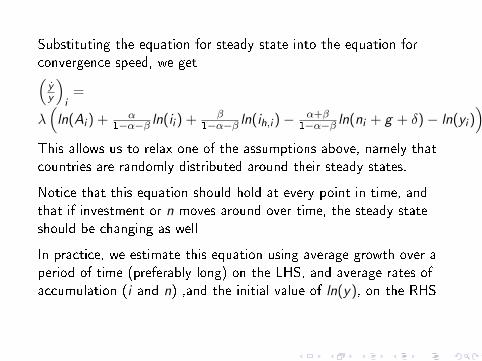
Substituting the equation for steady state into the equation forconvergence speed, we get(yy

)i

=

λ(ln(Ai ) + α

1−α−β ln(ii ) + β1−α−β ln(ih,i ) − α+β

1−α−β ln(ni + g + δ) − ln(yi ))

This allows us to relax one of the assumptions above, namely thatcountries are randomly distributed around their steady states.

Notice that this equation should hold at every point in time, andthat if investment or n moves around over time, the steady stateshould be changing as well

In practice, we estimate this equation using average growth over aperiod of time (preferably long) on the LHS, and average rates ofaccumulation (i and n) ,and the initial value of ln(y), on the RHS

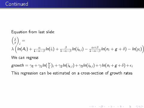
Continued

Equation from last slide:(yy

)i

=

λ(ln(Ai ) + α

1−α−β ln(ii ) + β1−α−β ln(ih,i ) − α+β

1−α−β ln(ni + g + δ) − ln(yi ))

We can regress

growth = γ0 +γ1ln(YL )i +γ2ln(ik,i )+γ3ln(ih,i )+γln(ni +g +δ)+εi

This regression can be estimated on a cross-section of growth rates

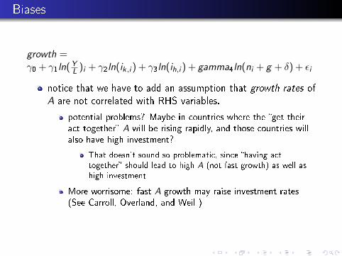
Biases

growth =γ0 + γ1ln(YL )i + γ2ln(ik,i ) + γ3ln(ih,i ) + gamma4ln(ni + g + δ) + εi

notice that we have to add an assumption that growth rates ofA are not correlated with RHS variables.

potential problems? Maybe in countries where the �get theiract together� A will be rising rapidly, and those countries willalso have high investment?

That doesn't sound so problematic, since �having acttogether� should lead to high A (not fast growth) as well ashigh investment

More worrisome: fast A growth may raise investment rates(See Carroll, Overland, and Weil )

Left Hand Side Variable

In the speci�cation I derived, the left hand side variable wasthe growth rate of output

Most cross-country regression work uses the average growth

rate of output (over some period) on the LHS

MRW used the change in the log of output on the LHS. Thismatters (a bit) because the model implies that growth shouldbe slowing down over time.

Result is that MRW can't just interpret the coe�cient oninitial income (γ1) as an estimate of −λ. Instead, they have todo an adjustment for the number of years in the period.

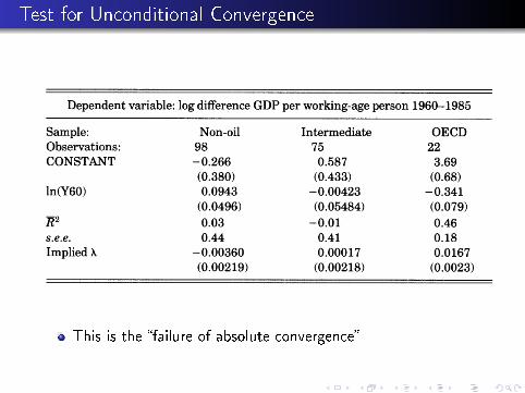
Test for Unconditional Convergence

This is the �failure of absolute convergence�

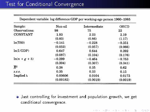
Test for Conditional Convergence

Just controlling for investment and population growth, we getconditional convergence.

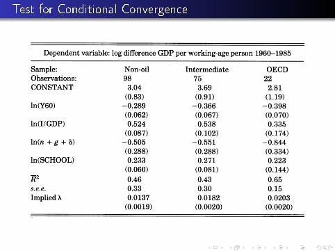
Test for Conditional Convergence

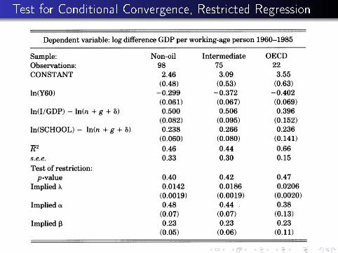
Test for Conditional Convergence, Restricted Regression

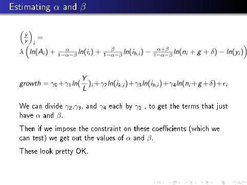
Estimating α and β

(yy

)i

=

λ(ln(Ai ) + α

1−α−β ln(ii ) + β1−α−β ln(ih,i ) − α+β

1−α−β ln(ni + g + δ) − ln(yi ))

growth = γ0+γ1ln(Y

L)i +γ2ln(ik,i )+γ3ln(ih,i )+γ4ln(ni +g +δ)+εi

We can divide γ2,γ3, and γ4 each by γ1 , to get the terms that justhave α and β.

Then if we impose the constraint on these coe�cients (which wecan test) we get out the values of α and β.

These look pretty OK.

Convergence

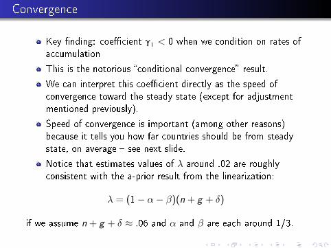
Key �nding: coe�cient γ1 < 0 when we condition on rates ofaccumulation

This is the notorious �conditional convergence� result.

We can interpret this coe�cient directly as the speed ofconvergence toward the steady state (except for adjustmentmentioned previously).

Speed of convergence is important (among other reasons)because it tells you how far countries should be from steadystate, on average � see next slide.

Notice that estimates values of λ around .02 are roughlyconsistent with the a-prior result from the linearization:

λ = (1− α− β)(n + g + δ)

if we assume n + g + δ ≈ .06 and α and β are each around 1/3.

Speed of Approach to Steady State

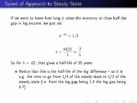
If we want to know how long it takes the economy to close half thegap in log income, we just set

e−λt = 1/2

t =ln(2)

λ≈ .7

λ

So for λ = .02, that gives a half-life of 35 years.

Notice that this is the half-life of the log di�erence � so it ise.g. the time to go from 1/4 of the steady state to 1/2 of thesteady state [i.e. from the log gap being 1.4 the log gap being0.7]

Adding Other Stu� to the RHS of Growth Regresions

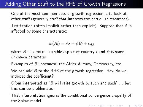
One of the most common uses of growth regression is to look atother stu� (generally stu� that interests the particular researcher)

Justi�cation (often implicit rather than explicit): Suppose that A isa�ected by some characteristic:

ln(Ai ) = A0 + ψBi + εA,i

where B is some measurable aspect of country i and ψ is someunknown parameter

Examples of B : openness, the Africa dummy, Democracy, etc.

We can add B to the RHS of the growth regression. How do weinterpet the coe�cient?

Often interpreted as �B will raise growth by such and such� ... butthis can be problematic

That interpretation ignores the conditional convergence property ofthe Solow model.

Adding Other Stu� to RHS of Growth Regressions

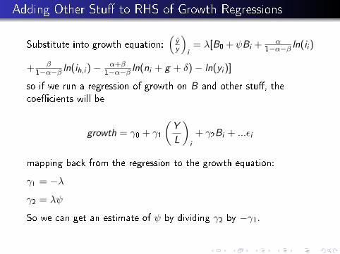
Substitute into growth equation:(yy

)i

= λ[B0 +ψBi + α1−α−β ln(ii )

+ β1−α−β ln(ih,i ) − α+β

1−α−β ln(ni + g + δ) − ln(yi )]

so if we run a regression of growth on B and other stu�, thecoe�cients will be

growth = γ0 + γ1

(Y

L

)i

+ γ2Bi + ...εi

mapping back from the regression to the growth equation:

γ1 = −λ

γ2 = λψ

So we can get an estimate of ψ by dividing γ2 by −γ1.

The right interpretation of the coe�cient on B is that �doing suchand such raises the steady state level of income by this amount,and that there is transitional growth toward this new steady state.Once in the new steady state, it does not a�ect growth.�

What if the �other stu�� a�ected something other thanproductivity, like investment, human capital accumulation, etc?

Then it shouldn't be on the RHS of the growth regression atall.

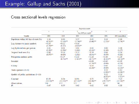
Example: Gallup and Sachs (2001)

Cross sectional levels regression

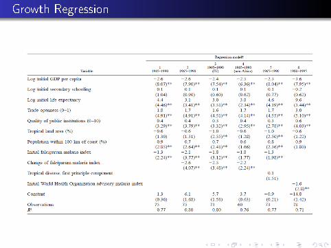
Growth Regression

Interpretation of Coe�cients

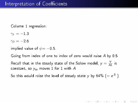
Column 1 regression:

γ1 = −1.3

γ2 = −2.6

implied value of ψ= −0.5.

Going from index of one to index of zero would raise A by 0.5

Recall that in the steady state of the Solow model, y = YAL is

constant, so yss moves 1 for 1 with A

So this would raise the level of steady state y by 64% (= e .5 )

Abuja Declaration

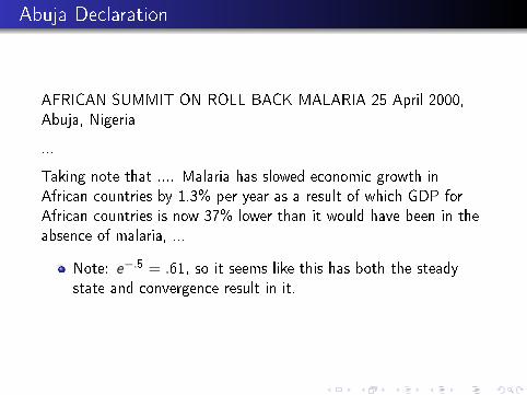
AFRICAN SUMMIT ON ROLL BACK MALARIA 25 April 2000,Abuja, Nigeria

...

Taking note that .... Malaria has slowed economic growth inAfrican countries by 1.3% per year as a result of which GDP forAfrican countries is now 37% lower than it would have been in theabsence of malaria, ...

Note: e−.5 = .61, so it seems like this has both the steadystate and convergence result in it.

General Problems with Regressions

I look at applications to growth regressions

we do identi�cation last

Problem #1: Omitted Variables

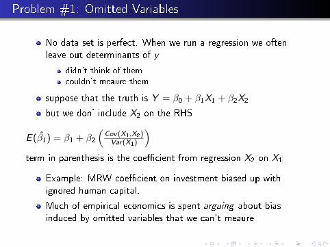
No data set is perfect. When we run a regression we oftenleave out determinants of y

didn't think of themcouldn't meaure them

suppose that the truth is Y = β0 + β1X1 + β2X2

but we don' include X2 on the RHS

E (β1) = β1 + β2

(Cov(X1,X2)Var(X1)

)term in parenthesis is the coe�cient from regression X2 on X1

Example: MRW coe�cient on investment biased up withignored human capital.

Much of empirical economics is spent arguing about biasinduced by omitted variables that we can't meaure

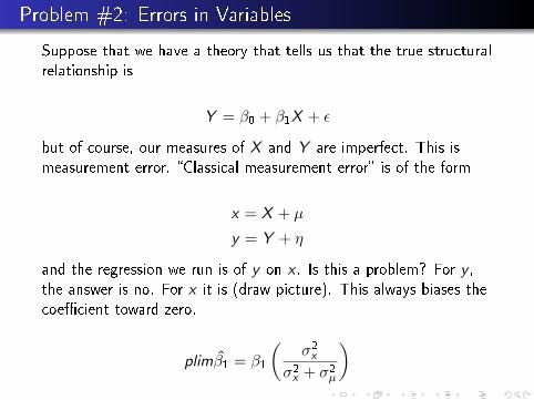
Problem #2: Errors in Variables

Suppose that we have a theory that tells us that the true structuralrelationship is

Y = β0 + β1X + ε

but of course, our measures of X and Y are imperfect. This ismeasurement error. �Classical measurement error� is of the form

x = X + µ

y = Y + η

and the regression we run is of y on x . Is this a problem? For y ,the answer is no. For x it is (draw picture). This always biases thecoe�cient toward zero.

plimβ1 = β1

(σ2x

σ2x + σ2µ

)

Bias in Other Coe�cients

Another problem comes when measurement error biases othercoe�cients. Take the case where the true relationship is

Y = β0 + β1X1 + β2X2 + ε

where β1 > 0 and corr(X1,X2) > 0

Suppose that X1 is measured with lots of error but X2 is not.

Then β2 will be biased upward. This is really just a case of omittedvariable bias, since the measurement error in X1is making it as ifthat variable was not included.

Classic example from outside of growth: regress income oneducation and race (dummy for black). Education is in years, butthis is a poor meaure of true education, since quality varies. Thecoe�cient on race is picking up both true race e�ect (holdingeducation constant) and correlation of race with unmeasurededucation quality (I guess that is not classical measurement error).

Example from growth literature: including the Africa dummy,quality of government, etc. on RHS of cross-country regression.

According to discussion above, if we already have investment,schooling, etc. on the RHS, then these things coming insigni�cantly is evidence that they a�ect productivity.

But all those things are measured poorly, so Africa dummy etc.could be picking up non-productivity e�ects.

Note: IV can �x bias from measurement error. You can eveninstrument for one noisy measure with another (if their errors areuncorrelated) to get rid of bias.

Problem #3: Spatial Issues

There are lots of reasons to think that neighboring countriesin�uence each other. How will that a�ect econometrics?

Consider two adjacent countries, i and j

yi = βXi + εi

yj = βXj + εj

Two possible issues:

correlation of the ε terms. This might occur if there were someunmeasured variable that enters the true model that we arenot including on the RHS, and if that variable had ageographic component

examples: climate, disease environment, natural resources,some aspect of history, etc.

Spatial Issues � continued

Either X or ε from a neighboring country a�ects outcomes in acountry. This is a spillover or externality e�ect

1 examples: schooling in one a�ects neighbor; quality ofinstitutions; political outcomes.

2 Much of thinking about endogenous growth stresses spilloversfrom investment that go from one �rm to another (so thesocial MPK is greater than the private). Natural to think thatthese spillovers go across countries as well.

Spatial Issues

The �rst problem is called �spatial correlation� (or sometimes�spatial autocorrelation�). Closely analagous to serialcorrelation in time series.

biases standard errors downward but does not bias coe�cients.can correct for spatial correlation if you have a �map� of whatis next to whatin the time domain this is easy (t is next to t − 1, etc.) but forspatial stu� it is a bit harder.

Spillovers are much harder to deal with.

You still need some kind of spatial mapyou also potentially have to deal with �re�ection� ininterpreting coe�cients

Chua: �Regional Spillovers and Economic Growth�

look at how neighbors's physical and human capital a�ectsown output

Production function is key innovation:

y = kαhβkεRhεR

where the R subscript denotes the regional average

note the unpleasant assumption that averages rather thantotals are what matter. Nothing in this model says that livingin a crowded neighborhood is better. But if you really believedin spillovers, it should be.

Implementation of regions: each country's �region� is theaverage of all countries it touches.

no adjustment for size of neighbors, i.e. Guatemala and USmatter equally for Mexicono adjustment for size relative to neighbors, i.e. region mattersjust as much for US as for Luxembourg

Chua, continued

Rest of the model is just like MRW

Chua goes through the algebra of the Solow model with hisproduction function

Steady state level of income is function of own and neighbors' ratesof investement (physical and human capital) and populationgrowth.

As in MRW, can run regressions in either levels or growth rates.

Note re�ection issue: a high value of Ai , ik , or ih raises k andh in a country, which raises output in neighboring countries,which raises k and h in those countries, which raises output incountry i .

it is not 100% clear to me that Chua dealt with this correctly(and the paper is not published).

Possible Interesting Things to Find

suppose externality were big: then you could have EndogenousGrowth even though coe�cients in individual countries do notjustify it.

could �nd that some kinds of investment have biggerexternalities that others (e.g. humans vs. machines).

maybe spillovers will allow for elimination of continentdummies. Maybe the common factor in Africa is being in abad neigborhood.

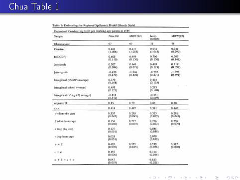
Chua Table 1

Table 1 Findings

regression in levels

Taken separately, only weak evidence of spillovers (one sig.coe�cient in non-oil sample)

but when you add spillover coe�cients, the sum is sign�cantlydi�erent than zero

[note: it might be interesting to calculate productivity usingdevelopment accounting and put the value of that for neighbors onthe RHS as well]

Table 4

This is the growth regression

adding regional variables largely eliminates the continentdummies.

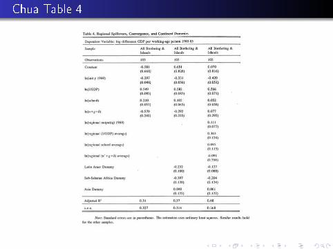
Chua Table 4

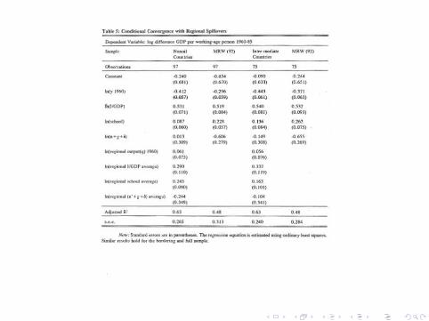
Table 5

Compares regional model to MRW

Regional model �ts better, but there are weird things withcoe�cients

estimates say that regional schooling matters more than own?!

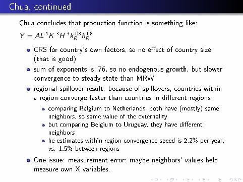
Chua, continued

Chua concludes that production function is something like:

Y = AL.4K .3H .3k .08R h.08R

CRS for country's own factors, so no e�ect of country size(that is good)

sum of exponents is .76, so no endogenous growth, but slowerconvergence to steady state than MRW

regional spillover result: because of spillovers, countries withina region converge faster than countries in di�erent regions

comparing Belgium to Netherlands, both have (mostly) sameneighbors, so same value of the externalitybut comparing Belgium to Uruguay, they have di�erentneighborshe estimates within region convergence speed is 2.2% per year,vs. 1.5% between regions

One issue: measurement error: maybe neighbors' values helpmeasure own X variables.

Problem #4: Outliers

A big drawback of cross-country empirical work is smallnumber of observations

If you are going to work with data like this, you must look tosee if a couple of in�uential observations are determining yourkey estimates.

In fact, you should do this all the time, but it is particularyimportant in cross-country and similar work.

What to do:

If you have one variable on the RHS, just make a scatterplotIf you have more than one RHS variable, see next page

Looking for Outliers

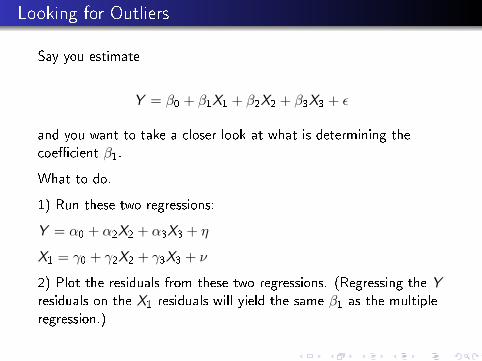
Say you estimate

Y = β0 + β1X1 + β2X2 + β3X3 + ε

and you want to take a closer look at what is determining thecoe�cient β1.

What to do.

1) Run these two regressions:

Y = α0 + α2X2 + α3X3 + η

X1 = γ0 + γ2X2 + γ3X3 + ν

2) Plot the residuals from these two regressions. (Regressing the Yresiduals on the X1 residuals will yield the same β1 as the multipleregression.)

What to do When You Find In�uential Outliers

Worry: do the in�uential observations share some commonfactor that, if you put it in the regression, would make theresult go away?

If yes, is it credible that this common factor would a�ect Ydirectly?

Also: do the outlier observations have a high value of X forthe same reason?

Application: East Asian Dragons

William Easterly, �Explaining Miracles: Growth RegressionsMeet the Gang of Four� (1995)

Intensive investigation of East Asian outliers in growthregression (Hong Kong, S. Korea, Singapore, Taiwan)

Goal is to understand if we should trust coe�cient oninvestment rate (and other inferences from regressions).

Worry: maybe there is a �Confucian ethic� that made themsave more also made them richer .

East Asian Dragons

Easterly says no:

Though they have geographical and cultural proximity, thereare other countries (Burma, Indonesia, Philippines, Vietnam)that could also fall into this category.ex-ante, no one thought of these countries as a group. Sogrouping them now may be observer bias.

also funny stories about how World Bank thought that S.Korea was bound to fail while Philippines and sub SaharanAfrica were likely to succeed, etc.

My view: subsequent fast growth of China + Putterman andWeil results say that maybe there is something in common.

Problem #5: Robustness

Lots of people write papers along the following lines:

1 I have a theory that X should matter for the level (or growthrate) of output

2 I put X on the RHS of a growth regression

3 X comes in signi�cant

4 publish paper

Levine and Renelt worry about this approach. Problem is thatputting other people's X variables on the right hand side mightmake mine insigni�cant.

They implement �extreme bounds analysis,� orginally developed byLeamer.

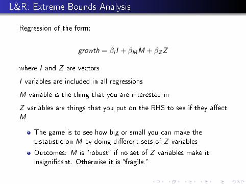
L&R: Extreme Bounds Analysis

Regression of the form:

growth = βi I + βMM + βZZ

where I and Z are vectors

I variables are included in all regressions

M variable is the thing that you are interested in

Z variables are things that you put on the RHS to see if they a�ectM

The game is to see how big or small you can make thet-statistic on M by doing di�erent sets of Z variables

Outcomes: M is �robust� if no set of Z variables make itinsigni�cant. Otherwise it is �fragile.�

Ground Rules for EBA

The set of potential Z variables is all the stu� that otherpeople have put on the RHS of growth regressions

they had about 50

They use up to three at a time

Z variables are grouped by conceptual classes (e.g. monetary,�scal, etc.). They do not include Z variables from the sameclass as the M variable being tested.

They try all possible combinations

I Variables

Table 1 does sensitivity results for the variables that willbecome the I variables.

initial income, investment, population growth, secondaryschool enrollment

three out of four are robust (not population growth)

Table lists the combinations of Z variables that give highestand lowest t-stats.

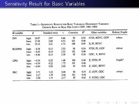
Sensitivity Result for Basic Variables

L&R Main Results

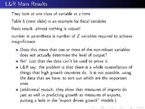
They look at one class of variable at a time

Table 6 (next slide) is an example for �scal variables

Basic result: almost nothing is robust!

number in parenthesis is number of Z variables required to achieveinsigni�cance

Does this mean that one or more of the non-robust variablesdoes not actually determine the level of output?

No! Just that the data can't be used to prove it.

L&R say: the problem is that there is a whole constellation ofthings that high growth countries do. It is not possible, usingthe data that we have, to sort out which are the importantones.

(additional reusult: they show that measures of imports dojust as well in predicting growth as measures of exports,putting a hole in the �export driven growth� models.)

The L&R Vision

There should be a standard set of Z variables

People writing papers would report robustness w.r.t. those Zvariables for every regression

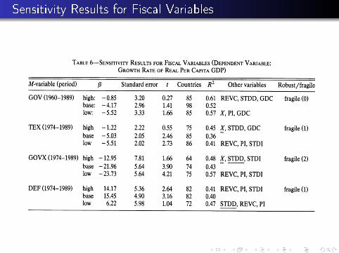
Sensitivity Results for Fiscal Variables

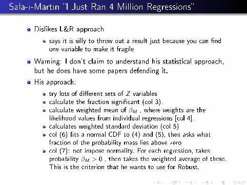
Sala-i-Martin �I Just Ran 4 Million Regressions�

Dislikes L&R approach

says it is silly to throw out a result just because you can �ndone variable to make it fragile

Warning: I don't claim to understand his statistical approach,but he does have some papers defending it.

His approach:

try lots of di�erent sets of Z variablescalculate the fraction signi�cant (col 3).calculate weighted mean of βM , where weights are thelikelihood values from individual regressions [col 4].calculates weighted standard deviation (col 5)col (6) �ts a normal CDF to (4) and (5), then asks whatfraction of the probability mass lies above zerocol (7): not impose normality. For each regression, takesprobability βM > 0 , then takes the weighted average of these.This is the criterion that he wants to use for Robust.

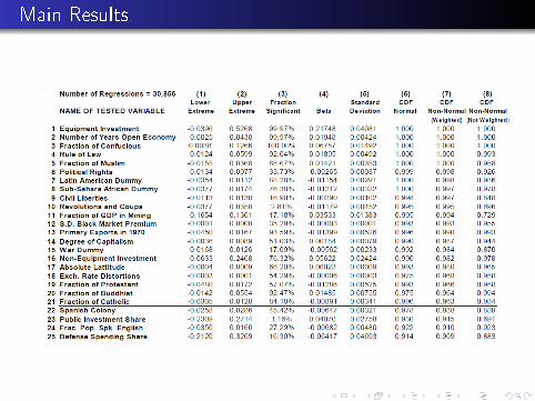
Main Results

Robustness Continued

Sala-i-Martin �nds many regressors are robust in his sense.

one problem: procedure is dependent on list of regressors used.Adding junk to this list raises the probability of robustness.

The Sad Conclusion of Robustness

The L&R procedure was not adopted

possibly because there was not agreed-upon list of z variablespossibly because it was too destructive of published results

The Sala-i-Martin proposal never went anywhere

What we actually do:

z variables added by intuition, insistence of referees, desire tocite friends, etc.very easy to maniupulateunsatisfactory

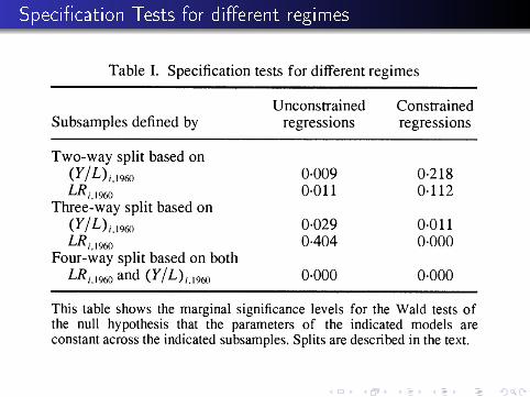
Speci�cation Tests for di�erent regimes

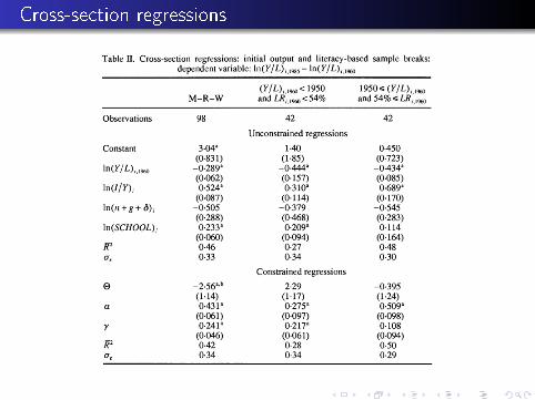
Cross-section regressions

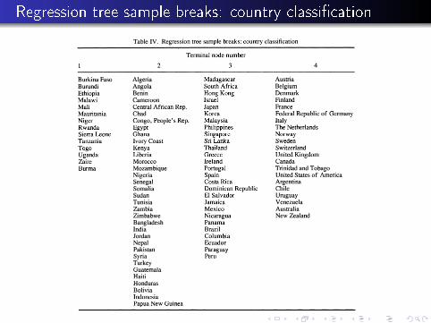
Regression tree sample breaks: country classi�cation

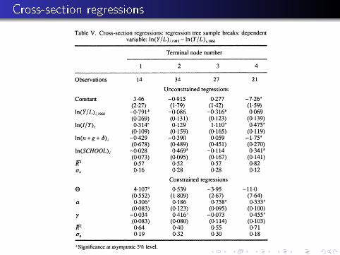
Cross-section regressions

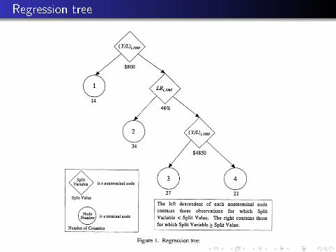
Regression tree