USING MATRIX ALGEBRA TO UNDERSTAND POPULATION

GROWTH RATE

GEOFF SMITH AND LEWIS D. LUDWIG

Abstract. This module introduces students to the use of matrix algebra inpopulation ecology. In particular, it examines the construction of population

projection matrices from life table graphs, how the population projection ma-

trix can be used to determine population growth rates λ, and how manipulat-ing the population projection matrix can be used to determine which aspects

of the population projection matrix are most responsible for driving λ. This

module will allow students to gain a better understanding of 1) the underlyingmatrix algebra of population projection matrices, 2) the linkages between vi-

tal rates (e.g., survivorship, fecundity) and λ, 3) relationships between stableage distributions and λ, and 4) the use of life table response experiments to

determine the importance of each vital rate for determining λ.

1. Overview

This module is designed for two populations of students. One target group isstudents in an introductory finite mathematics course and the other populationis students in an upper-level course in ecology [2]. Completion of the modulerequires no prior knowledge of matrix algebra, nor does it assume prior knowledgeof population growth models or life tables. Thus, this module is appropriate foreither a finite mathematics or ecology course.

To make the module as accessible as possible, the module includes a MicrosoftExcel R© spreadsheet that allows students to explore the computation of λ and sta-ble age distributions, as well as to conduct life table response experiments: Age-BasedEx.xlsx, StableAgeDistribution.xlsx.

2. Introduction: Life Tables

For population ecologists and conservation biologists one of the most importantparameters to understanding population dynamics is the population growth rate.A population growth rate is determined by the birth or fecundity rate, the number ofbabies born in a given time, and death or mortality rate, the number of individualsdying in a given time.

While it might appear fairly easy to find the fecundity rate and mortality rateof a population, the population ecologists job of understanding the dynamics of a

Key words and phrases. population growth rate, life table, life graph, fecundity, survivorship,stable age distribution, matrix, eigenvector.

This work was supported by National Science Foundation (9952806).

1

2 GEOFF SMITH AND LEWIS D. LUDWIG

population is made difficult by the fact that both the birth rate and the death ratefor an individual can change over the course of its life, and this change can haveimplications for how fast a population grows.

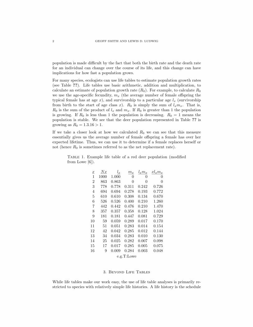
For many species, ecologists can use life tables to estimate population growth rates(see Table ??). Life tables use basic arithmetic, addition and multiplication, tocalculate an estimate of population growth rate (R0). For example, to calculate R0

we use the age-specific fecundity, mx (the average number of female offspring thetypical female has at age x), and survivorship to a particular age lx (survivorshipfrom birth to the start of age class x). R0 is simply the sum of lxmx. That is,R0 is the sum of the product of lx and mx. If R0 is greater than 1 the populationis growing. If R0 is less than 1 the population is decreasing. R0 = 1 means thepopulation is stable. We see that the deer population represented in Table ?? isgrowing as R0 = 1.3.16 > 1.

If we take a closer look at how we calculated R0 we can see that this measureessentially gives us the average number of female offspring a female has over herexpected lifetime. Thus, we can use it to determine if a female replaces herself ornot (hence R0 is sometimes referred to as the net replacement rate).

Table 1. Example life table of a red deer population (modifiedfrom Lowe [6]).

x Nx lx mx lxmx xlxmx

1 1000 1.000 0 0 02 863 0.863 0 0 03 778 0.778 0.311 0.242 0.7264 694 0.694 0.278 0.193 0.7725 610 0.610 0.308 0.134 0.6706 526 0.526 0.400 0.210 1.2607 442 0.442 0.476 0.210 1.4708 357 0.357 0.358 0.128 1.0249 181 0.181 0.447 0.081 0.729

10 59 0.059 0.289 0.017 0.17011 51 0.051 0.283 0.014 0.15412 42 0.042 0.285 0.012 0.14413 34 0.034 0.283 0.010 0.13014 25 0.025 0.282 0.007 0.09815 17 0.017 0.285 0.005 0.07516 9 0.009 0.284 0.003 0.048

e.g.T:Lowe

3. Beyond Life Tables

While life tables make our work easy, the use of life table analyses is primarily re-stricted to species with relatively simple life histories. A life history is the schedule

USING MATRIX ALGEBRA TO UNDERSTAND POPULATION GROWTH RATE 3

Seed Age 1

TransitionProbability

Fecundity

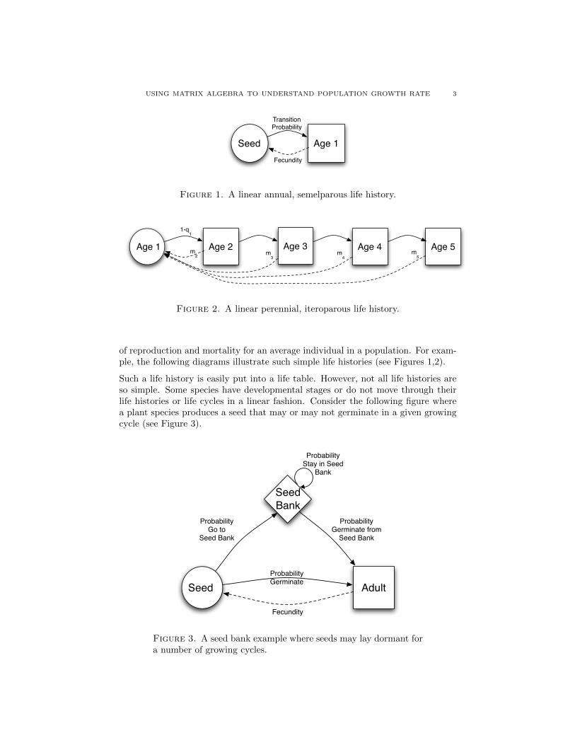
Figure 1. A linear annual, semelparous life history.

Age 1 Age 2

1-q1

Age 3 Age 4 Age 5m2 m

3m4

m5

Figure 2. A linear perennial, iteroparous life history.

of reproduction and mortality for an average individual in a population. For exam-ple, the following diagrams illustrate such simple life histories (see Figures 1,2).

Such a life history is easily put into a life table. However, not all life histories areso simple. Some species have developmental stages or do not move through theirlife histories or life cycles in a linear fashion. Consider the following figure wherea plant species produces a seed that may or may not germinate in a given growingcycle (see Figure 3).

Seed Adult

Fecundity

ProbabilityGerminate

Seed Bank

ProbabilityStay in Seed

Bank

ProbabilityGerminate from

Seed Bank

ProbabilityGo to

Seed Bank

Figure 3. A seed bank example where seeds may lay dormant fora number of growing cycles.

4 GEOFF SMITH AND LEWIS D. LUDWIG

Another interesting example is the stage-based life cycle where individuals aregrouped according to the stage of their life cycle as opposed to age. For exam-ple, consider Figure 4 which represents the life cycle of frogs. An individual isplaced in a stage and has a certain probability of remaining in that stage and acertain probability of moving to the next stage. It should be noted that an individ-ual can only move one stage at a time and that sequence of developmental stagesis not reversible.

Egg Large AdultTadpole Juvenile Small

Adult

Figure 4. Frogs demonstrate a stage-based life cycle.

Similarly, there is a size-based life cycle, where an individual is in a particular sizeclass and has a certain probability of moving to the next size class or remaining inthe current size class. We assume no individual can move more than one size classper growing cycle. Certain species of fish are a natural example of this life cycle.

4. The Power of Linear Algebra

While certain life histories are conducive to using life tables to estimate populationgrowth rates, as we have seen in Section 3, many are not. Fortunately, we can usematrix or linear algebra to examine population growth in such species. We can alsouse matrix algebra to figure out what aspects of the life history are most influentialon the population growth rate, which is particularly useful for trying to conservespecies and populations.

4.1. Example: The Matrix Model.

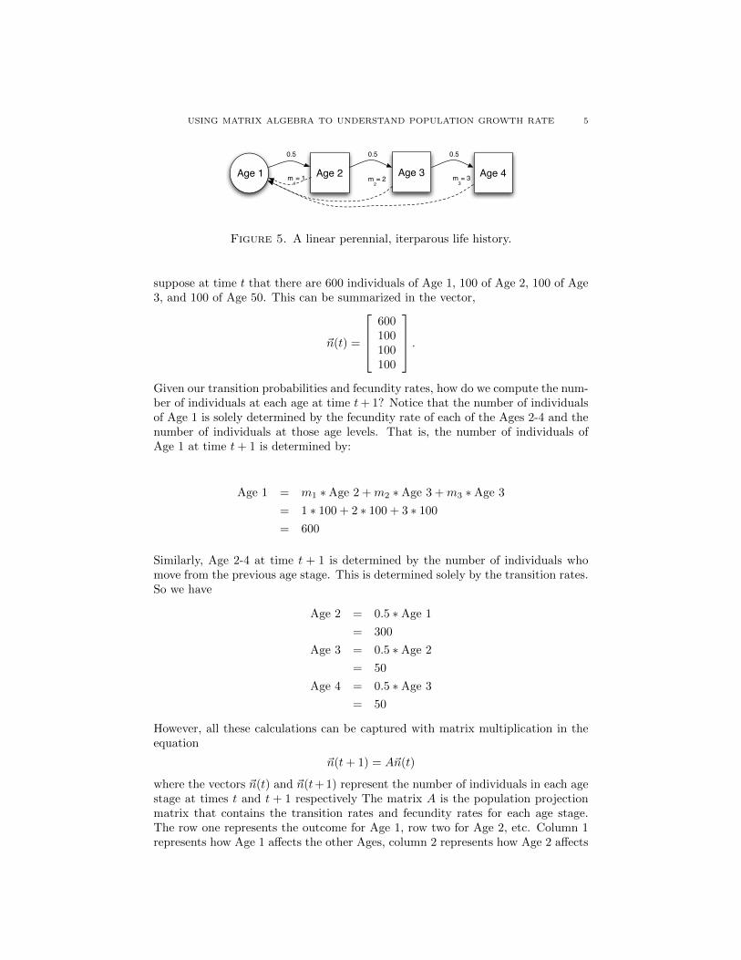
To see how matrix algebra can be used in population models, we consider thefollowing example. Suppose we have a population that models a linear perennial,iteroparous life history (i.e., an individual lives more than one year and reproducesmore than once) with four ages, Age 1-4. The probability of an individual movingfrom Age 1 to Age 2, Age 2 to Age 3, or Age 3 to Age 4 is each 0.5. We also havethe following age-specific fecundity rates: m1 = 1, m2 = 2, and m3 = 3. This lifecycle is modeled in Figure 7.

This figure is more than a useful pictorial description of the life cycle. We cancapture this information using matrix algebra. Let ~n(t) represent the vector thatcontains the number of individuals in each life stage, Age 1-4. For our example,

USING MATRIX ALGEBRA TO UNDERSTAND POPULATION GROWTH RATE 5

Age 1 Age 2

0.5

Age 3 Age 4m1= 1

0.5 0.5

m2= 2 m

3= 3

Figure 5. A linear perennial, iterparous life history.

suppose at time t that there are 600 individuals of Age 1, 100 of Age 2, 100 of Age3, and 100 of Age 50. This can be summarized in the vector,

~n(t) =

600100100100

.Given our transition probabilities and fecundity rates, how do we compute the num-ber of individuals at each age at time t+ 1? Notice that the number of individualsof Age 1 is solely determined by the fecundity rate of each of the Ages 2-4 and thenumber of individuals at those age levels. That is, the number of individuals ofAge 1 at time t+ 1 is determined by:

Age 1 = m1 ∗ Age 2 +m2 ∗ Age 3 +m3 ∗ Age 3

= 1 ∗ 100 + 2 ∗ 100 + 3 ∗ 100

= 600

Similarly, Age 2-4 at time t + 1 is determined by the number of individuals whomove from the previous age stage. This is determined solely by the transition rates.So we have

Age 2 = 0.5 ∗ Age 1

= 300

Age 3 = 0.5 ∗ Age 2

= 50

Age 4 = 0.5 ∗ Age 3

= 50

However, all these calculations can be captured with matrix multiplication in theequation

~n(t+ 1) = A~n(t)

where the vectors ~n(t) and ~n(t+ 1) represent the number of individuals in each agestage at times t and t + 1 respectively The matrix A is the population projectionmatrix that contains the transition rates and fecundity rates for each age stage.The row one represents the outcome for Age 1, row two for Age 2, etc. Column 1represents how Age 1 affects the other Ages, column 2 represents how Age 2 affects

6 GEOFF SMITH AND LEWIS D. LUDWIG

the other Ages, etc. For example, if we allow t = 0, we have the following.

~n(1) = A~n(0)

=

0 1 2 3

0.5 0 0 00 0.5 0 00 0 0.5 0

600100100100

=

6003005050

Question 1. How would we use ~n(1) to compute ~n(2), that is the population ofeach stage at time 2?

As you can see, the calculations to project population sizes into the future are rela-tively simple, if tedious, using basic matrix algebra. Using a computer to do thesemultiple iterations will be much faster and much less tedious. Before we try this,let’s first get some more practice with creating population projection matrices andlife cycle graphs.

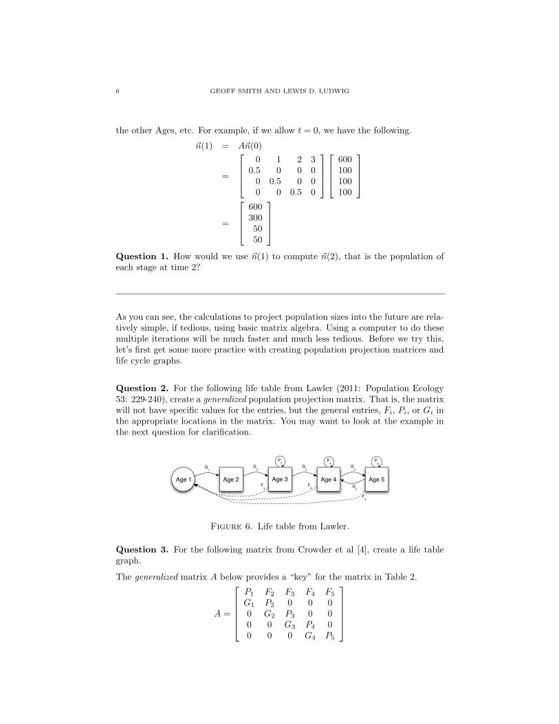
Question 2. For the following life table from Lawler (2011: Population Ecology53: 229-240), create a generalized population projection matrix. That is, the matrixwill not have specific values for the entries, but the general entries, Fi, Pi, or Gi inthe appropriate locations in the matrix. You may want to look at the example inthe next question for clarification.

Age 1 Age 2 Age 3 Age 4 Age 5F

3F

4

F5

G1

G2

G3

G4

G5

P3

P4

P5

Figure 6. Life table from Lawler.

Question 3. For the following matrix from Crowder et al [4], create a life tablegraph.

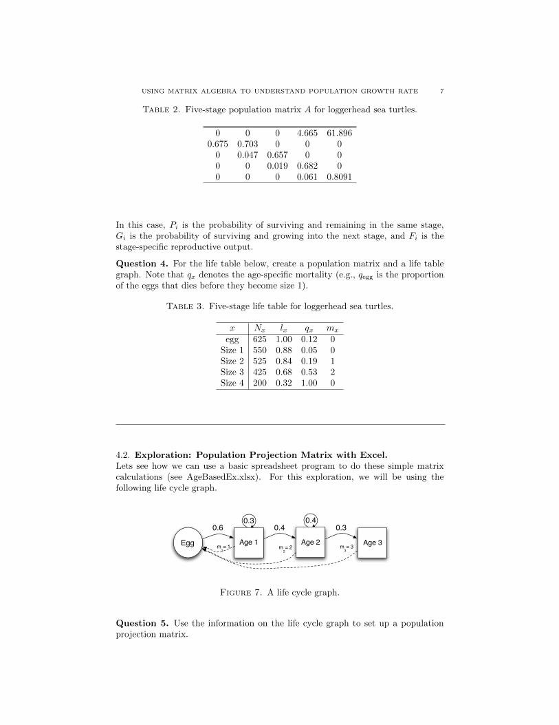
The generalized matrix A below provides a “key” for the matrix in Table 2.

A =

P1 F2 F3 F4 F5

G1 P2 0 0 00 G2 P3 0 00 0 G3 P4 00 0 0 G4 P5

USING MATRIX ALGEBRA TO UNDERSTAND POPULATION GROWTH RATE 7

Table 2. Five-stage population matrix A for loggerhead sea turtles.

0 0 0 4.665 61.8960.675 0.703 0 0 0

0 0.047 0.657 0 00 0 0.019 0.682 00 0 0 0.061 0.8091

In this case, Pi is the probability of surviving and remaining in the same stage,Gi is the probability of surviving and growing into the next stage, and Fi is thestage-specific reproductive output.

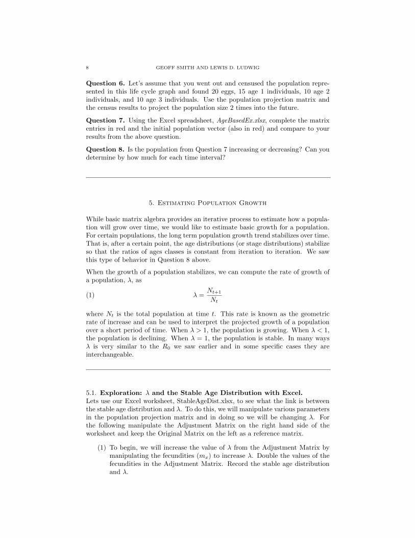
Question 4. For the life table below, create a population matrix and a life tablegraph. Note that qx denotes the age-specific mortality (e.g., qegg is the proportionof the eggs that dies before they become size 1).

Table 3. Five-stage life table for loggerhead sea turtles.

x Nx lx qx mx

egg 625 1.00 0.12 0Size 1 550 0.88 0.05 0Size 2 525 0.84 0.19 1Size 3 425 0.68 0.53 2Size 4 200 0.32 1.00 0

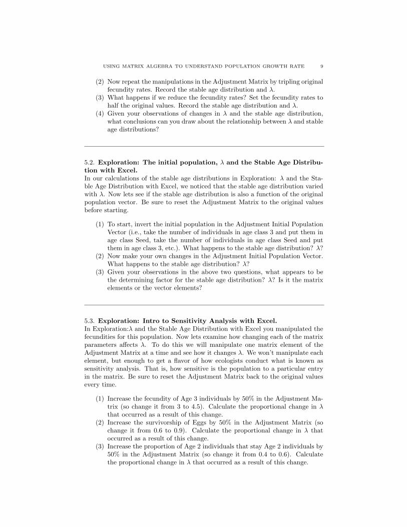
4.2. Exploration: Population Projection Matrix with Excel.Lets see how we can use a basic spreadsheet program to do these simple matrixcalculations (see AgeBasedEx.xlsx). For this exploration, we will be using thefollowing life cycle graph.

Egg Age 1 Age 2

0.6 0.4 0.30.3 0.4

Age 3 m1= 1 m

2= 2 m

3= 3

Figure 7. A life cycle graph.

Question 5. Use the information on the life cycle graph to set up a populationprojection matrix.

8 GEOFF SMITH AND LEWIS D. LUDWIG

Question 6. Let’s assume that you went out and censused the population repre-sented in this life cycle graph and found 20 eggs, 15 age 1 individuals, 10 age 2individuals, and 10 age 3 individuals. Use the population projection matrix andthe census results to project the population size 2 times into the future.

Question 7. Using the Excel spreadsheet, AgeBasedEx.xlsx, complete the matrixentries in red and the initial population vector (also in red) and compare to yourresults from the above question.

Question 8. Is the population from Question 7 increasing or decreasing? Can youdetermine by how much for each time interval?

5. Estimating Population Growth

While basic matrix algebra provides an iterative process to estimate how a popula-tion will grow over time, we would like to estimate basic growth for a population.For certain populations, the long term population growth trend stabilizes over time.That is, after a certain point, the age distributions (or stage distributions) stabilizeso that the ratios of ages classes is constant from iteration to iteration. We sawthis type of behavior in Question 8 above.

When the growth of a population stabilizes, we can compute the rate of growth ofa population, λ, as

(1) λ =Nt+1

Nt

where Nt is the total population at time t. This rate is known as the geometricrate of increase and can be used to interpret the projected growth of a populationover a short period of time. When λ > 1, the population is growing. When λ < 1,the population is declining. When λ = 1, the population is stable. In many waysλ is very similar to the R0 we saw earlier and in some specific cases they areinterchangeable.

5.1. Exploration: λ and the Stable Age Distribution with Excel.Lets use our Excel worksheet, StableAgeDist.xlsx, to see what the link is betweenthe stable age distribution and λ. To do this, we will manipulate various parametersin the population projection matrix and in doing so we will be changing λ. Forthe following manipulate the Adjustment Matrix on the right hand side of theworksheet and keep the Original Matrix on the left as a reference matrix.

(1) To begin, we will increase the value of λ from the Adjustment Matrix bymanipulating the fecundities (mx) to increase λ. Double the values of thefecundities in the Adjustment Matrix. Record the stable age distributionand λ.

USING MATRIX ALGEBRA TO UNDERSTAND POPULATION GROWTH RATE 9

(2) Now repeat the manipulations in the Adjustment Matrix by tripling originalfecundity rates. Record the stable age distribution and λ.

(3) What happens if we reduce the fecundity rates? Set the fecundity rates tohalf the original values. Record the stable age distribution and λ.

(4) Given your observations of changes in λ and the stable age distribution,what conclusions can you draw about the relationship between λ and stableage distributions?

5.2. Exploration: The initial population, λ and the Stable Age Distribu-tion with Excel.In our calculations of the stable age distributions in Exploration: λ and the Sta-ble Age Distribution with Excel, we noticed that the stable age distribution variedwith λ. Now lets see if the stable age distribution is also a function of the originalpopulation vector. Be sure to reset the Adjustment Matrix to the original valuesbefore starting.

(1) To start, invert the initial population in the Adjustment Initial PopulationVector (i.e., take the number of individuals in age class 3 and put them inage class Seed, take the number of individuals in age class Seed and putthem in age class 3, etc.). What happens to the stable age distribution? λ?

(2) Now make your own changes in the Adjustment Initial Population Vector.What happens to the stable age distribution? λ?

(3) Given your observations in the above two questions, what appears to bethe determining factor for the stable age distribution? λ? Is it the matrixelements or the vector elements?

5.3. Exploration: Intro to Sensitivity Analysis with Excel.In Exploration:λ and the Stable Age Distribution with Excel you manipulated thefecundities for this population. Now lets examine how changing each of the matrixparameters affects λ. To do this we will manipulate one matrix element of theAdjustment Matrix at a time and see how it changes λ. We won’t manipulate eachelement, but enough to get a flavor of how ecologists conduct what is known assensitivity analysis. That is, how sensitive is the population to a particular entryin the matrix. Be sure to reset the Adjustment Matrix back to the original valuesevery time.

(1) Increase the fecundity of Age 3 individuals by 50% in the Adjustment Ma-trix (so change it from 3 to 4.5). Calculate the proportional change in λthat occurred as a result of this change.

(2) Increase the survivorship of Eggs by 50% in the Adjustment Matrix (sochange it from 0.6 to 0.9). Calculate the proportional change in λ thatoccurred as a result of this change.

(3) Increase the proportion of Age 2 individuals that stay Age 2 individuals by50% in the Adjustment Matrix (so change it from 0.4 to 0.6). Calculatethe proportional change in λ that occurred as a result of this change.

10 GEOFF SMITH AND LEWIS D. LUDWIG

(4) Which element had the greatest impact on λ? How did you come to thatconclusion?

One issue with using Equation 1 to compute λ is that it can only be done oncea stable age distribution has been reached. In other words, we would have toiteratively find the age distributions until the ratios of the age, or stage, classes isconstant from iteration to iteration.

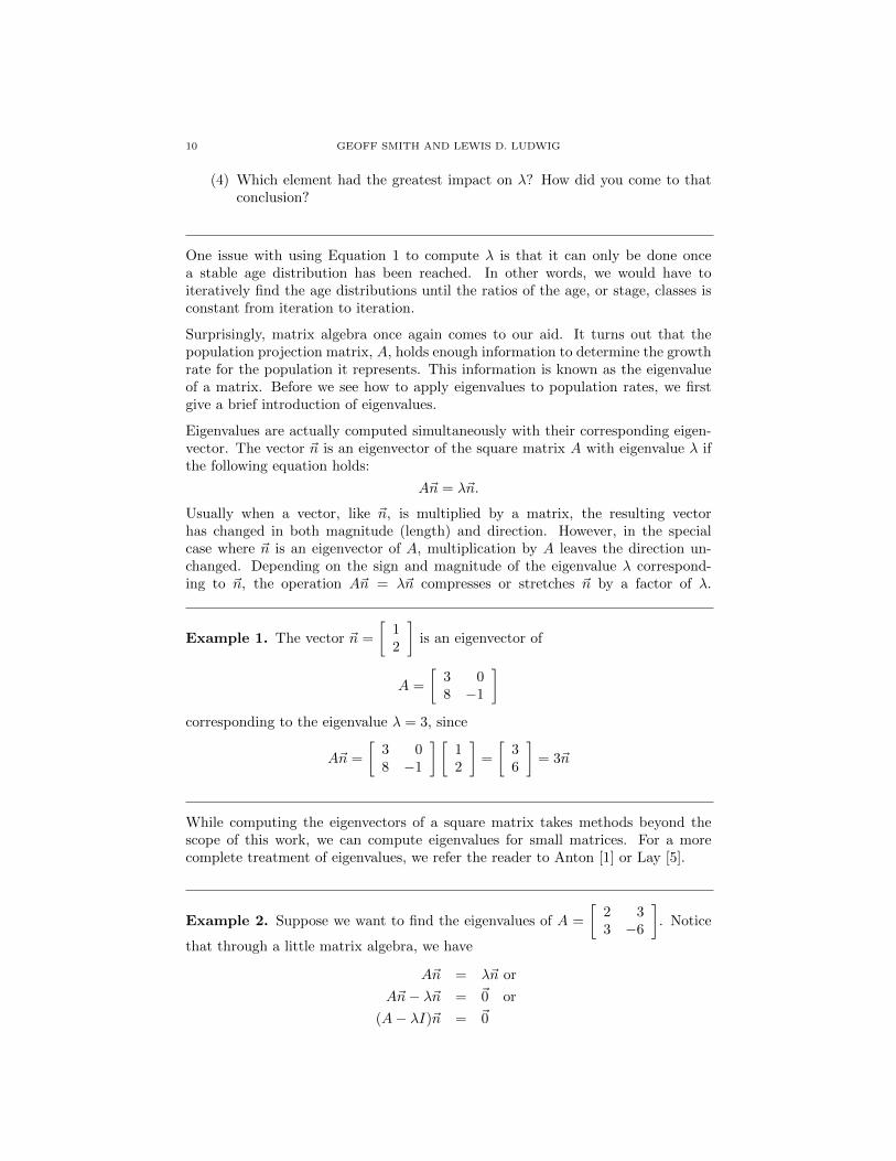
Surprisingly, matrix algebra once again comes to our aid. It turns out that thepopulation projection matrix, A, holds enough information to determine the growthrate for the population it represents. This information is known as the eigenvalueof a matrix. Before we see how to apply eigenvalues to population rates, we firstgive a brief introduction of eigenvalues.

Eigenvalues are actually computed simultaneously with their corresponding eigen-vector. The vector ~n is an eigenvector of the square matrix A with eigenvalue λ ifthe following equation holds:

A~n = λ~n.

Usually when a vector, like ~n, is multiplied by a matrix, the resulting vectorhas changed in both magnitude (length) and direction. However, in the specialcase where ~n is an eigenvector of A, multiplication by A leaves the direction un-changed. Depending on the sign and magnitude of the eigenvalue λ correspond-ing to ~n, the operation A~n = λ~n compresses or stretches ~n by a factor of λ.

Example 1. The vector ~n =

[12

]is an eigenvector of

A =

[3 08 −1

]corresponding to the eigenvalue λ = 3, since

A~n =

[3 08 −1

] [12

]=

[36

]= 3~n

While computing the eigenvectors of a square matrix takes methods beyond thescope of this work, we can compute eigenvalues for small matrices. For a morecomplete treatment of eigenvalues, we refer the reader to Anton [1] or Lay [5].

Example 2. Suppose we want to find the eigenvalues of A =

[2 33 −6

]. Notice

that through a little matrix algebra, we have

A~n = λ~n or

A~n− λ~n = ~0 or

(A− λI)~n = ~0

USING MATRIX ALGEBRA TO UNDERSTAND POPULATION GROWTH RATE 11

Since the eigenvector ~n must be nonzero and (A − λI)~n = ~0, by the InvertibleMatrix1 Theorem, we need (A − λI) to be non-invertible. Otherwise, if (A − λI)was invertible, then we would have ~n = 0. For our example, we now have

A− λI =

[2 33 −6

]−[λ 00 λ

]=

[2 − λ 3

3 −6 − λ

].

We have seen that a matrix is not invertible if its determinant is zero. We want tofind λ such that the determinant of (A − λI) is zero. So the eigenvalues of A arethe solutions of the equation

det(A− λI) = det

[2 − λ 3

3 −6 − λ

]= 0.

Recall that

det

[a bc d

]= ad− bc.

So

det(A− λI) = (2 − λ)(−6 − λ) − (3)(3)

= −12 + 6λ− 2λ+ λ2 − 9

= λ2 + 4λ− 21

= (λ− 3)(λ+ 7).

If det(A− λI) = 0, then λ = 3 or λ = −7. So the eigenvalues of A are 3 and -7.

While finding the eigenvalues for a 2 × 2 matrix reduces to solving a quadraticequation, as the size of the matrix increase, so does the degree of the accompanyingpolynomial (known as the characteristic polynomial). So to find the eigenvalues of a4× 4 matrix, we would have to solve a fourth degree polynomial, i.e., a polynomialwith λ4 terms. In general, this is a very difficult task. Luckily, we can turn totechnology for help.

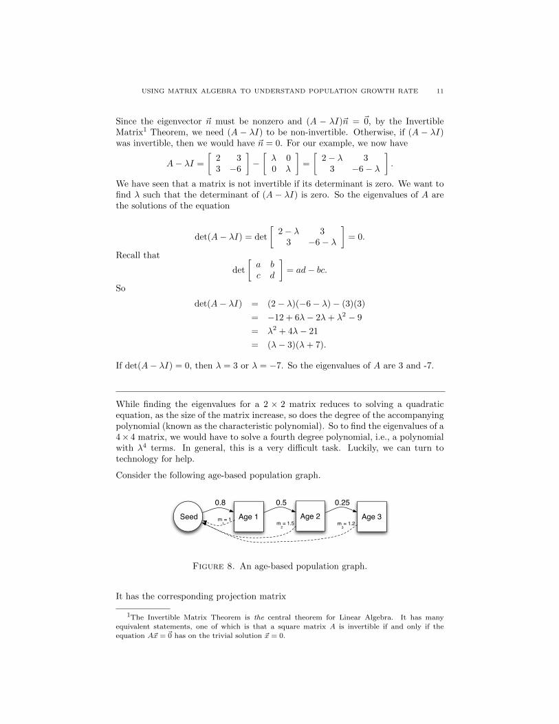
Consider the following age-based population graph.

Seed Age 1

0.8

Age 2 Age 3

0.5 0.25

m1= 1

m2= 1.5 m

3= 1.2

Figure 8. An age-based population graph.

It has the corresponding projection matrix

1The Invertible Matrix Theorem is the central theorem for Linear Algebra. It has many

equivalent statements, one of which is that a square matrix A is invertible if and only if the

equation A~x = ~0 has on the trivial solution ~x = 0.

12 GEOFF SMITH AND LEWIS D. LUDWIG

A =

0 1 1.5 1.2

0.8 0 0 00 0.5 0 00 0 0.25 0

To consider the long term behavior of this population, would could iterate An~n(0)until the age distributions stabilize. Instead, we will compute the eigenvalues ofthis matrix. Since this is a 4 × 4 matrix, we can have up to four eigenvalues. Tocompute this we use the web-based program WolframAlpha R© to find the eigenvaluesare approximately 1.18, -0.31, -0.43+0.36i, and -0.43-0.36i, please see Figure 9. Sowhich value determines the population growth? Also, notice that some of the valuesare imaginary? First, imaginary solutions come with the territory. Even simplequadratic equations such as x2 + 4 = 0 have imaginary solutions. With regard towhich of the four values we use, we choose the one with the largest magnitude,which in this case is λ = 1.18. The eigenvalue with the largest magnitude is knownas the dominant eigenvalue. For those interested in why the dominant eigenvalueis the one that determines the rate of growth in the population, we refer to you toCaswell [3].

Figure 9. Using WolframAlpha to compute eigenvalues.

References

[1] Anton, Howard and Rorres, Chris 2010. Elementary Linear Algebra, Tenth Edition. John

Wiley and Sons, Inc., Hoboken, NJ.[2] Cain, M.L., W.D. Bowman, and S.D. Hacker. 2011. Ecology, 2nd Edition. Sinauer Associates,

Sunderland, MA.[3] Caswell, Hal, 2001. Matrix Population Models: Construction, Analysis, and Interpretation,

Second Edition. Sinauer Associates, Inc., Suderland, MA.

[4] Crowder, Larry B., Deborah T. Crouse, Selina S. Heppell, and Thomas H. Martin. Predictingthe Impact of Turtle Excluder Devices on Loggerhead Sea Turtle Populations. 1994 EcologicalApplications 4:437445.

USING MATRIX ALGEBRA TO UNDERSTAND POPULATION GROWTH RATE 13

[5] Lay, David 2011. Linear Algebra and Its Applications, Fourth Edition. AddisonWesley, Boston,

MA.

[6] Lowe, V.P.W., Population dynamics of the red deer (Cervus elaphus L.) on Rhum, 1969Journal of Animal Ecology 38: 425-457.

2011, Department of Biology and Department of Mathematics and Computer Science,

Denison University, Granville, OH 43023 smithg@denison.edu, ludwigl@denison.edu