Combinatorics of Triangulations and the Chern-Simons Invariant for Hyperbolic 3-Manifolds

Hyperbolic volume, Mahler measure, and homologygrowth
Thang Le
School of MathematicsGeorgia Institute of Technology
Columbia University, June 2009
Outline
1 Homology Growth and volume
2 Torsion and Determinant
3 L2-Torsion
4 Approximation by finite groups

Outline
1 Homology Growth and volume
2 Torsion and Determinant
3 L2-Torsion
4 Approximation by finite groups

Finite covering of knot complement
K is a knot in S3, X = S3 \ K , π = π1(X ).
π is residually finite: ∃ a nested sequence of normal subgroups
π = G0 ⊃ G1 ⊃ G2 . . .
[π : Gk ] < ∞, ∩kGk = {1}.
If [π : G] < ∞, let XG = G-covering of X
X brG = branched G-covering of S3
Want: Asymptotics of H1(X brGk
, Z) as k →∞
.
Finite covering of knot complement
K is a knot in S3, X = S3 \ K , π = π1(X ).
π is residually finite: ∃ a nested sequence of normal subgroups
π = G0 ⊃ G1 ⊃ G2 . . .
[π : Gk ] < ∞, ∩kGk = {1}.
If [π : G] < ∞, let XG = G-covering of X
X brG = branched G-covering of S3
Want: Asymptotics of H1(X brGk
, Z) as k →∞.

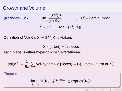
Growth and Volume
(Kazhdan-Luck) limk→∞
b1(X brGk
)
[π : Gk ]= 0 (= L2 − Betti number).
t(K , G) := |TorH1(XbrG , Z)|.
Definition of Vol(K ): X = S3 \ K is Haken.
X \ (t tori) = tpieces
each piece is either hyperbolic or Seifert-fibered.
Vol(K ) :=1
6π
∑Vol(hyperbolic pieces) = C(Gromov norm of X ).
Theorem
lim supk→∞
t(K , Gk )1/[π:Gk ] ≤ exp(Vol(K )).
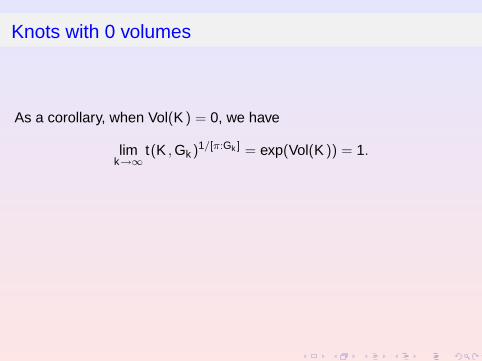
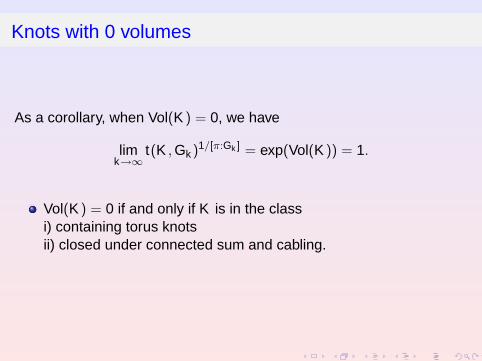
Knots with 0 volumes
As a corollary, when Vol(K ) = 0, we have
limk→∞
t(K , Gk )1/[π:Gk ] = exp(Vol(K )) = 1.
Vol(K ) = 0 if and only if K is in the classi) containing torus knotsii) closed under connected sum and cabling.
Knots with 0 volumes
As a corollary, when Vol(K ) = 0, we have
limk→∞
t(K , Gk )1/[π:Gk ] = exp(Vol(K )) = 1.
Vol(K ) = 0 if and only if K is in the classi) containing torus knotsii) closed under connected sum and cabling.
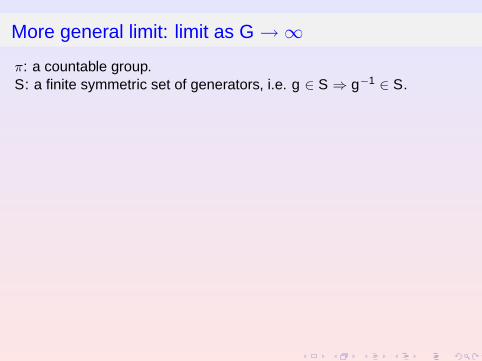
More general limit: limit as G →∞
π: a countable group.S: a finite symmetric set of generators, i.e. g ∈ S ⇒ g−1 ∈ S.
The length of x ∈ π:
`S(x) = smallest length of words representing x
S′: another symmetric set of generators. Then ∃k1, k2 > 0 s.t.
∀x ∈ π, k1`S(x) < `S′(x) < k2`S(x).
(`S and `S′ are quasi-isometric.)
It follows that
limn→∞
`S(xn) = ∞⇐⇒ limn→∞
`S′(xn) = ∞.

More general limit
For a subgroup G ⊂ π, let
diamS(G) = min{`S(g), g ∈ G \ {1}}.
f : a function defined on a set of finite index normal subgroups of π.
limdiamG→∞
f (G) = L
means there is S such that
limdiamSG→∞
f (G) = L.
Similarly, we can define
lim supdiamG→∞
f (G).
Remark: If limk→∞ diamG = ∞ then ∩Gk = {1} (co-final).
Homology Growth and Volume
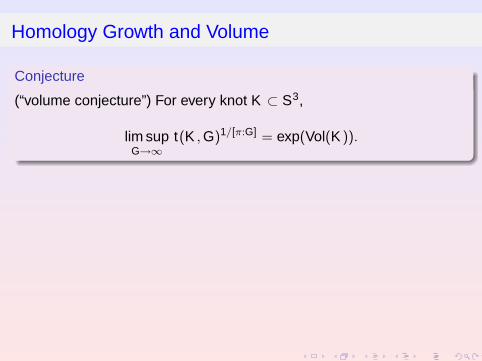
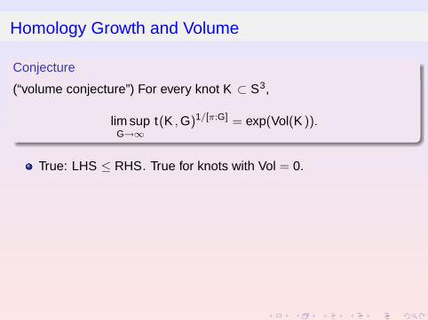
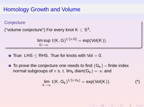
Conjecture
(“volume conjecture”) For every knot K ⊂ S3,
lim supG→∞
t(K , G)1/[π:G] = exp(Vol(K )).
True: LHS ≤ RHS. True for knots with Vol = 0.
To prove the conjecture one needs to find {Gk} – finite indexnormal subgroups of π s. t. limk diam(Gk ) = ∞ and
limk→∞
t(K , Gk )1/[π:Gk ] = exp(Vol(K )). (*)
It is unlikely that for any sequence Gk of normal subgroups s.t.lim diamGk = ∞ one has (*). Which {Gk} should we choose?
Homology Growth and Volume
Conjecture
(“volume conjecture”) For every knot K ⊂ S3,
lim supG→∞
t(K , G)1/[π:G] = exp(Vol(K )).
True: LHS ≤ RHS. True for knots with Vol = 0.
To prove the conjecture one needs to find {Gk} – finite indexnormal subgroups of π s. t. limk diam(Gk ) = ∞ and
limk→∞
t(K , Gk )1/[π:Gk ] = exp(Vol(K )). (*)
It is unlikely that for any sequence Gk of normal subgroups s.t.lim diamGk = ∞ one has (*). Which {Gk} should we choose?

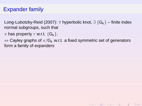
Expander family
Long-Lubotzky-Reid (2007): ∀ hyperbolic knot, ∃ {Gk} – finite indexnormal subgroups, such that
π has property τ w.r.t. {Gk}.
⇔ Cayley graphs of π/Gk w.r.t. a fixed symmetric set of generatorsform a family of expanders
⇔ the least non-zero eigenvalue of the Laplacian of the Cayley graphsof π/Gk is ≥ a fixed ε > 0.
Based on deep results of Bourgain-Gamburg (2007) on expandersfrom SL(2, p).
Conjecture
(*) holds for the Long-Lubotzky-Reid sequence {Gk}.
Justification: to follow.
Expander family
Long-Lubotzky-Reid (2007): ∀ hyperbolic knot, ∃ {Gk} – finite indexnormal subgroups, such that
π has property τ w.r.t. {Gk}.⇔ Cayley graphs of π/Gk w.r.t. a fixed symmetric set of generatorsform a family of expanders
⇔ the least non-zero eigenvalue of the Laplacian of the Cayley graphsof π/Gk is ≥ a fixed ε > 0.
Based on deep results of Bourgain-Gamburg (2007) on expandersfrom SL(2, p).
Conjecture
(*) holds for the Long-Lubotzky-Reid sequence {Gk}.
Justification: to follow.
Outline
1 Homology Growth and volume
2 Torsion and Determinant
3 L2-Torsion
4 Approximation by finite groups
Reidemeister Torsion
C: Chain complex of finite dimensional C-modules (vector spaces).
0 → Cn∂n→ Cn−1
∂n−1→ . . . C1∂1→ C0 → 0.
Suppose C is acyclic and based. Then the torsion τ(C) is defined.
ci : base of Ci . Each ∂i is given by a matrix.
Simplest case: C is 0 → C1∂1→ C0 → 0.
τ(C) = det ∂1.
0 → C2∂2→ C1
∂1→ C0 → 0.
τ(C) =
[∂2(c2)∂
−1c0
c1
]Here [a/b] is the determinant of the change matrix from b to a.

Torsion of chain of Hilbert spaces
C: complex of finite dimensional Hilbert spaces over C; acyclic.Choose orthonormal base ci for each Ci , define τ(C, c).
Change of base: τ(C) := |τ(C, c)| is well-defined.
C: complex of Hilbert spaces over C[π]. Want to define τ(C).
0 → Cn∂n→ Cn−1
∂n−1→ . . . C1∂1→ C0 → 0.
More specifically,
Ci = Z[π]ni , free Z[π]−module, or Ci = `2(π)ni
∂i ∈ Mat(ni × ni−1, Z[π]), acting on the right.
Need to define what is the determinant of a matrixA ∈ Mat(m × n, Z[π]).

Trace on C[π]
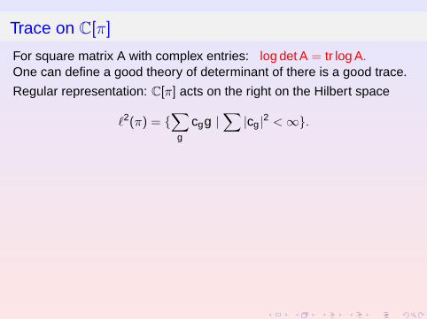
For square matrix A with complex entries: log det A = tr log A.One can define a good theory of determinant of there is a good trace.
Regular representation: C[π] acts on the right on the Hilbert space
`2(π) = {∑
g
cgg |∑
|cg |2 < ∞}.
Remark. If π = π1(S3 \ K ), K is not a torus knot, then the regularrepresentation is of type II1.
Adjoint operator: x =∑
cgg ∈ C[π], then x∗ =∑
cgg−1.
Similarly to the finite group case, define ∀g ∈ π,
tr(g) = δg,1
∀x ∈ C[π], tr(x) = 〈x , 1〉 = coeff. of 1 in x .
Trace on C[π]
For square matrix A with complex entries: log det A = tr log A.One can define a good theory of determinant of there is a good trace.
Regular representation: C[π] acts on the right on the Hilbert space
`2(π) = {∑
g
cgg |∑
|cg |2 < ∞}.
Remark. If π = π1(S3 \ K ), K is not a torus knot, then the regularrepresentation is of type II1.
Adjoint operator: x =∑
cgg ∈ C[π], then x∗ =∑
cgg−1.
Similarly to the finite group case, define ∀g ∈ π,
tr(g) = δg,1
∀x ∈ C[π], tr(x) = 〈x , 1〉 = coeff. of 1 in x .
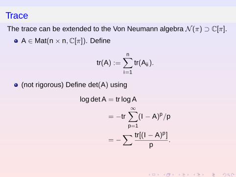
TraceThe trace can be extended to the Von Neumann algebra N (π) ⊃ C[π].
A ∈ Mat(n × n, C[π]). Define
tr(A) :=n∑
i=1
tr(Aii).
(not rigorous) Define det(A) using
log det A = tr log A
= −tr∞∑
p=1
(I − A)p/p
= −∑ tr[(I − A)p]
p.
Convergence of the RHS?

TraceThe trace can be extended to the Von Neumann algebra N (π) ⊃ C[π].
A ∈ Mat(n × n, C[π]). Define
tr(A) :=n∑
i=1
tr(Aii).
(not rigorous) Define det(A) using
log det A = tr log A
= −tr∞∑
p=1
(I − A)p/p
= −∑ tr[(I − A)p]
p.
Convergence of the RHS?
TraceThe trace can be extended to the Von Neumann algebra N (π) ⊃ C[π].
A ∈ Mat(n × n, C[π]). Define
tr(A) :=n∑
i=1
tr(Aii).
(not rigorous) Define det(A) using
log det A = tr log A
= −tr∞∑
p=1
(I − A)p/p
= −∑ tr[(I − A)p]
p.
Convergence of the RHS?

TraceThe trace can be extended to the Von Neumann algebra N (π) ⊃ C[π].
A ∈ Mat(n × n, C[π]). Define
tr(A) :=n∑
i=1
tr(Aii).
(not rigorous) Define det(A) using
log det A = tr log A
= −tr∞∑
p=1
(I − A)p/p
= −∑ tr[(I − A)p]
p.
Convergence of the RHS?
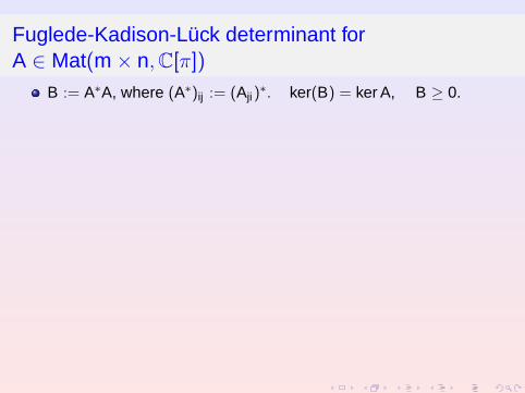
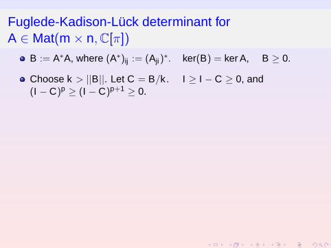
Fuglede-Kadison-Luck determinant forA ∈ Mat(m × n, C[π])
B := A∗A, where (A∗)ij := (Aji)∗. ker(B) = ker A, B ≥ 0.
Choose k > ||B||. Let C = B/k . I ≥ I − C ≥ 0, and(I − C)p ≥ (I − C)p+1 ≥ 0.
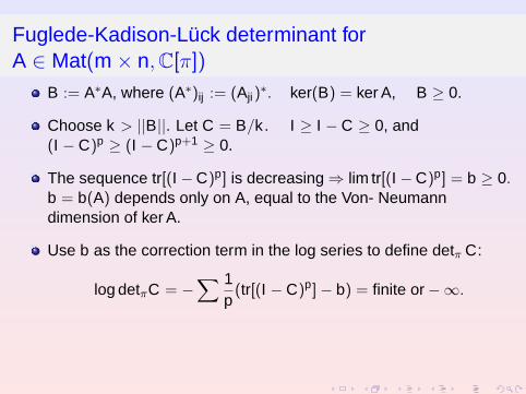
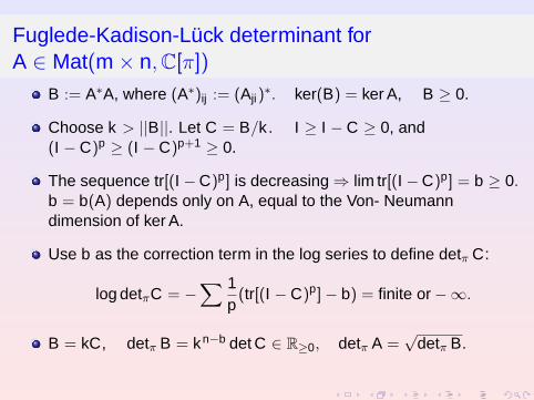
The sequence tr[(I −C)p] is decreasing ⇒ lim tr[(I −C)p] = b ≥ 0.b = b(A) depends only on A, equal to the Von- Neumanndimension of ker A.
Use b as the correction term in the log series to define detπ C:
log detπC = −∑ 1
p(tr[(I − C)p]− b) = finite or−∞.
B = kC, detπ B = kn−b det C ∈ R≥0, detπ A =√
detπ B.
Most interesting case: A is injective (b = 0), m = n, but not invertible.
Fuglede-Kadison-Luck determinant forA ∈ Mat(m × n, C[π])
B := A∗A, where (A∗)ij := (Aji)∗. ker(B) = ker A, B ≥ 0.
Choose k > ||B||. Let C = B/k . I ≥ I − C ≥ 0, and(I − C)p ≥ (I − C)p+1 ≥ 0.
The sequence tr[(I −C)p] is decreasing ⇒ lim tr[(I −C)p] = b ≥ 0.b = b(A) depends only on A, equal to the Von- Neumanndimension of ker A.
Use b as the correction term in the log series to define detπ C:
log detπC = −∑ 1
p(tr[(I − C)p]− b) = finite or−∞.
B = kC, detπ B = kn−b det C ∈ R≥0, detπ A =√
detπ B.
Most interesting case: A is injective (b = 0), m = n, but not invertible.

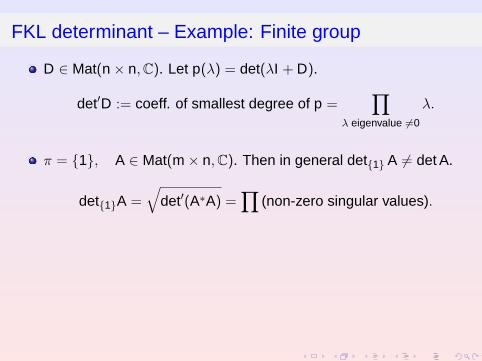
FKL determinant – Example: Finite group
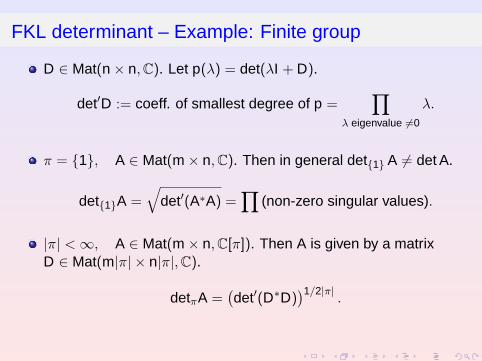
D ∈ Mat(n × n, C). Let p(λ) = det(λI + D).
det′D := coeff. of smallest degree of p =∏
λ eigenvalue 6=0
λ.
π = {1}, A ∈ Mat(m × n, C). Then in general det{1} A 6= det A.
det{1}A =√
det′(A∗A) =∏
(non-zero singular values).
|π| < ∞, A ∈ Mat(m × n, C[π]). Then A is given by a matrixD ∈ Mat(m|π| × n|π|, C).
detπA =(det′(D∗D)
)1/2|π|.
FKL determinant – Example: Finite group
D ∈ Mat(n × n, C). Let p(λ) = det(λI + D).
det′D := coeff. of smallest degree of p =∏
λ eigenvalue 6=0
λ.
π = {1}, A ∈ Mat(m × n, C). Then in general det{1} A 6= det A.
det{1}A =√
det′(A∗A) =∏
(non-zero singular values).
|π| < ∞, A ∈ Mat(m × n, C[π]). Then A is given by a matrixD ∈ Mat(m|π| × n|π|, C).
detπA =(det′(D∗D)
)1/2|π|.
FKL determinant– Example: π = Zµ
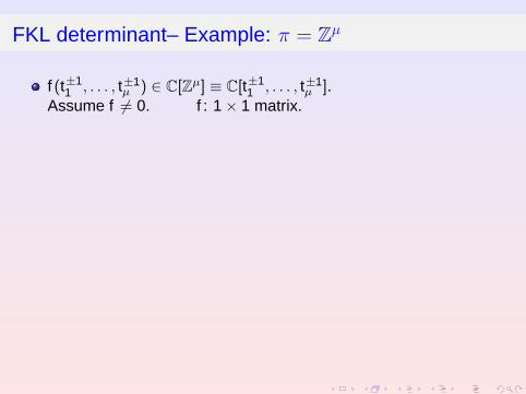
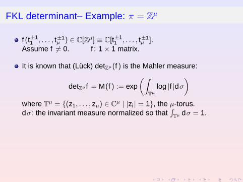
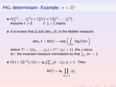
f (t±11 , . . . , t±1
µ ) ∈ C[Zµ] ≡ C[t±11 , . . . , t±1
µ ].Assume f 6= 0. f : 1× 1 matrix.
It is known that (Luck) detZµ(f ) is the Mahler measure:
detZµ f = M(f ) := exp(∫
Tµ
log |f |dσ
)where Tµ = {(z1, . . . , zµ) ∈ Cµ | |zi | = 1}, the µ-torus.dσ: the invariant measure normalized so that
∫Tµ dσ = 1.
f (t) ∈ Z[t±1], f (t) = a0∏n
j=1(t − zj), zj ∈ C. Then
M(f ) = a0
∏|zj |>1
|zj |.
FKL determinant– Example: π = Zµ
f (t±11 , . . . , t±1
µ ) ∈ C[Zµ] ≡ C[t±11 , . . . , t±1
µ ].Assume f 6= 0. f : 1× 1 matrix.
It is known that (Luck) detZµ(f ) is the Mahler measure:
detZµ f = M(f ) := exp(∫
Tµ
log |f |dσ
)where Tµ = {(z1, . . . , zµ) ∈ Cµ | |zi | = 1}, the µ-torus.dσ: the invariant measure normalized so that
∫Tµ dσ = 1.
f (t) ∈ Z[t±1], f (t) = a0∏n
j=1(t − zj), zj ∈ C. Then
M(f ) = a0
∏|zj |>1
|zj |.
Outline
1 Homology Growth and volume
2 Torsion and Determinant
3 L2-Torsion
4 Approximation by finite groups
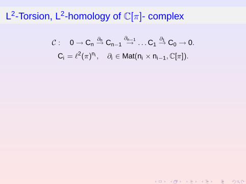
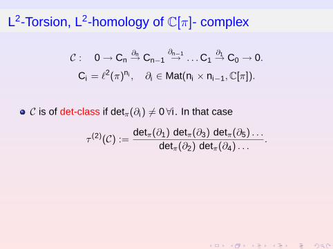
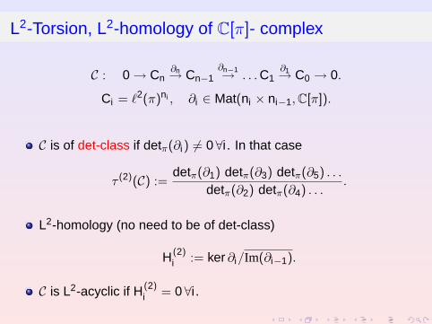
L2-Torsion, L2-homology of C[π]- complex
C : 0 → Cn∂n→ Cn−1
∂n−1→ . . . C1∂1→ C0 → 0.
Ci = `2(π)ni , ∂i ∈ Mat(ni × ni−1, C[π]).
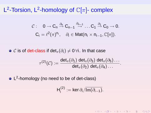
C is of det-class if detπ(∂i) 6= 0∀i . In that case
τ (2)(C) :=detπ(∂1) detπ(∂3) detπ(∂5) . . .
detπ(∂2) detπ(∂4) . . ..
L2-homology (no need to be of det-class)
H(2)i := ker ∂i/Im(∂i−1).
C is L2-acyclic if H(2)i = 0∀i .
L2-Torsion, L2-homology of C[π]- complex
C : 0 → Cn∂n→ Cn−1
∂n−1→ . . . C1∂1→ C0 → 0.
Ci = `2(π)ni , ∂i ∈ Mat(ni × ni−1, C[π]).
C is of det-class if detπ(∂i) 6= 0∀i . In that case
τ (2)(C) :=detπ(∂1) detπ(∂3) detπ(∂5) . . .
detπ(∂2) detπ(∂4) . . ..
L2-homology (no need to be of det-class)
H(2)i := ker ∂i/Im(∂i−1).
C is L2-acyclic if H(2)i = 0∀i .
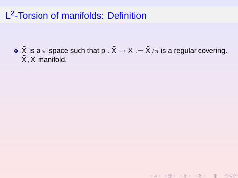
L2-Torsion of manifolds: Definition
X is a π-space such that p : X → X := X/π is a regular covering.X , X manifold.
Finite triangulation of X : C(X ) becomes a complex of freeZ[π]-modules.If C(X ) is of det-class, then L2-torsion, denoted by τ (2)(X ), can bedefined. Depends on the triangulation.
If C(X ) is acyclic and of det-class for one triangulation, then it isacyclic and of det-class for any other triangulation, and τ (2)(X ) ofthe two triangulations are the same: we can define τ (2)(X ).
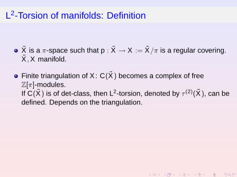
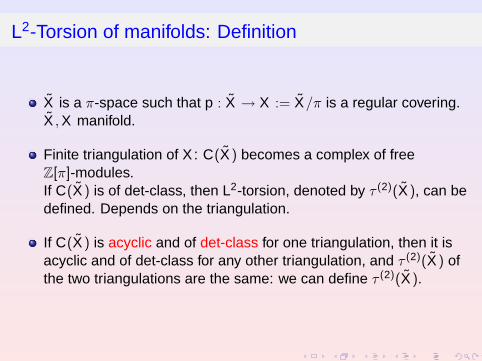
L2-Torsion of knots: universal covering
K a knot in S3. X = S3 − K , X : universal covering.π = π1(X ). Then X is a π-space with quotient X .
C(X ) is acyclic and is of det-class.
τ (2)(K ) := τ (2)(X ).
Theorem (Luck-Schick)
log τ (2)(K ) = −Vol(K ).
based on results of Burghelea-Friedlander-Kappeler-McDonald,Lott, and Mathai.
L2-Torsion of knots: computing using knot group
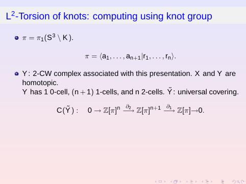
π = π1(S3 \ K ).
π = 〈a1, . . . , an+1|r1, . . . , rn〉.
Y : 2-CW complex associated with this presentation. X and Y arehomotopic.Y has 1 0-cell, (n +1) 1-cells, and n 2-cells. Y : universal covering.
C(Y ) : 0 → Z[π]n∂2−→ Z[π]n+1 ∂1−→ Z[π]→0.
∂1 =
a1 − 1a2 − 1
...an+1 − 1
, ∂2 =
(∂ri
∂aj
)∈ Mat(n × (n + 1), Z[π])
L2-Torsion of knots: computing using knot group
π = π1(S3 \ K ).
π = 〈a1, . . . , an+1|r1, . . . , rn〉.
Y : 2-CW complex associated with this presentation. X and Y arehomotopic.Y has 1 0-cell, (n +1) 1-cells, and n 2-cells. Y : universal covering.
C(Y ) : 0 → Z[π]n∂2−→ Z[π]n+1 ∂1−→ Z[π]→0.
∂1 =
a1 − 1a2 − 1
...an+1 − 1
, ∂2 =
(∂ri
∂aj
)∈ Mat(n × (n + 1), Z[π])
L2-Torsion of knots: computing using knot group
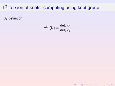
By definition
τ (2)(K ) =detπ ∂1
detπ ∂2
Let
∂′2 :=
(∂ri
∂aj
)n
i,j=1
∈ Mat(n × n, Z[π]).
Luck showed that
τ (2)(K ) =1
detπ ∂′2
It follows thatlog detπ(∂′2) = Vol(K ).

L2-Torsion of knots: computing using knot group
By definition
τ (2)(K ) =detπ ∂1
detπ ∂2
Let
∂′2 :=
(∂ri
∂aj
)n
i,j=1
∈ Mat(n × n, Z[π]).
Luck showed that
τ (2)(K ) =1
detπ ∂′2
It follows thatlog detπ(∂′2) = Vol(K ).

L2-Torsion of knots: computing using knot group
By definition
τ (2)(K ) =detπ ∂1
detπ ∂2
Let
∂′2 :=
(∂ri
∂aj
)n
i,j=1
∈ Mat(n × n, Z[π]).
Luck showed that
τ (2)(K ) =1
detπ ∂′2
It follows thatlog detπ(∂′2) = Vol(K ).
L2-Torsion of knots: Figure 8 knot
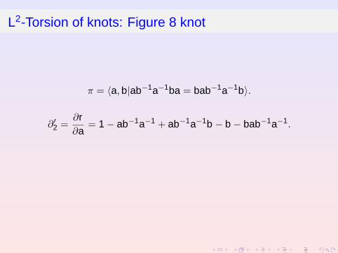
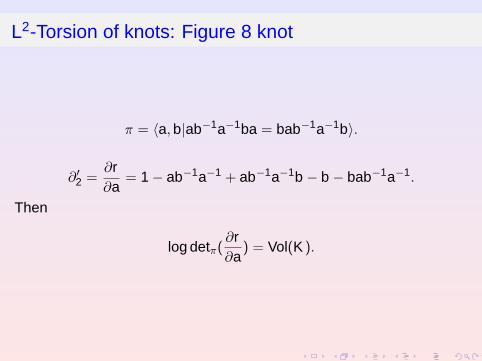
π = 〈a, b|ab−1a−1ba = bab−1a−1b〉.
∂′2 =∂r∂a
= 1− ab−1a−1 + ab−1a−1b − b − bab−1a−1.
Then
log detπ(∂r∂a
) = Vol(K ).
L2-Torsion of knots: Figure 8 knot
π = 〈a, b|ab−1a−1ba = bab−1a−1b〉.
∂′2 =∂r∂a
= 1− ab−1a−1 + ab−1a−1b − b − bab−1a−1.
Then
log detπ(∂r∂a
) = Vol(K ).

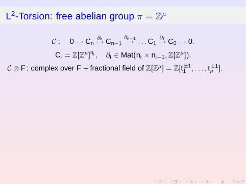
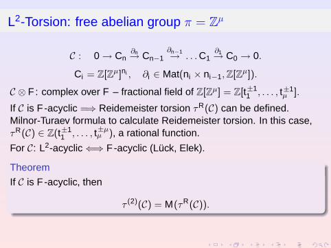
L2-Torsion: free abelian group π = Zµ
C : 0 → Cn∂n→ Cn−1
∂n−1→ . . . C1∂1→ C0 → 0.
Ci = Z[Zµ]ni , ∂i ∈ Mat(ni × ni−1, Z[Zµ]).
C ⊗ F : complex over F – fractional field of Z[Zµ] = Z[t±11 , . . . , t±1
µ ].
If C is F -acyclic =⇒ Reidemeister torsion τR(C) can be defined.Milnor-Turaev formula to calculate Reidemeister torsion. In this case,τR(C) ∈ Z(t±1
1 , . . . , t±µµ ), a rational function.
For C: L2-acyclic ⇐⇒ F -acyclic (Luck, Elek).
Theorem
If C is F -acyclic, then
τ (2)(C) = M(τR(C)).
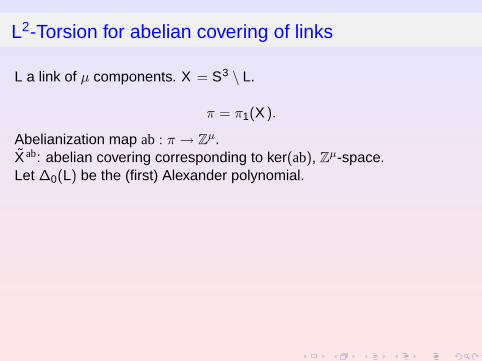
L2-Torsion for abelian covering of links
L a link of µ components. X = S3 \ L.
π = π1(X ).
Abelianization map ab : π → Zµ.X ab: abelian covering corresponding to ker(ab), Zµ-space.Let ∆0(L) be the (first) Alexander polynomial.
Proposition
C(X ab) is of det-class. C(X ab) is acyclic if and only if ∆0(L) 6= 0. If∆0(L) 6= 0
τ (2)(X ab) =1
M(∆0(L)).
If µ = 1, then ∆0 6= 0 always.

Outline
1 Homology Growth and volume
2 Torsion and Determinant
3 L2-Torsion
4 Approximation by finite groups
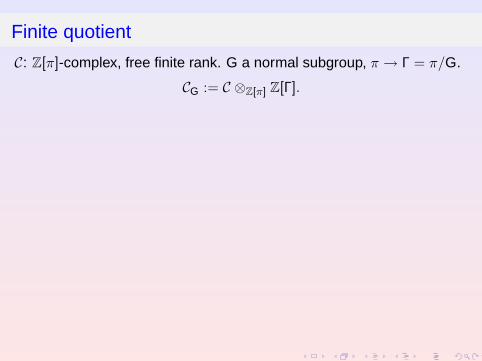
Finite quotient
C: Z[π]-complex, free finite rank. G a normal subgroup, π → Γ = π/G.
CG := C ⊗Z[π] Z[Γ].
If Γ is finite, then CG is a Z-complex of free finite rank Z-modules.
CG may not be acyclic even when C is. But the Betti numbers of CG are“small” compared to [π : G].
If CG is acyclic, then τR(CG) = t(C, G) (Milnor-Turaev formula),where
t(C, G) :=|TorH0(CG, Z)| |TorH2(CG, Z)| . . .|TorH1(CG, Z)| |TorH3(CG, Z)|
.
In general, limdiamG→∞
trπ/G(x) = trπ(x).
Question When
limdiamG→∞
t(C, G)1/[π:G] = τ (2)C?

Full result for π = Z
Theorem
π = Z. Gk = kZ ⊂ Z.
limk→∞
t(C, Gk )1/k = τ (2)C.
Proof of theorem used a special case, a result of Luck (Riley,Gonzalez-Acuna, and Short) based on Gelfond-Baker theory ofdiophantine approximation): f ∈ Q[Z], then
detZf = limn→∞
detZ/k (fZ/k )
and a result relating detZk to |Tor|.

Partial result π = Zµ
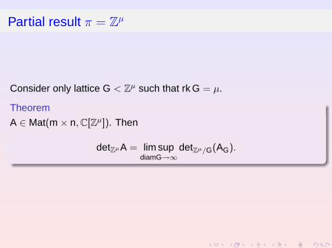
Consider only lattice G < Zµ such that rk G = µ.
Theorem
A ∈ Mat(m × n, C[Zµ]). Then
detZµA = lim supdiamG→∞
detZµ/G(AG).
Partial result π = Zµ
Consider only lattice G < Zµ such that rk G = µ.
Theorem
A ∈ Mat(m × n, C[Zµ]). Then
detZµA = lim supdiamG→∞
detZµ/G(AG).
Application: Link case
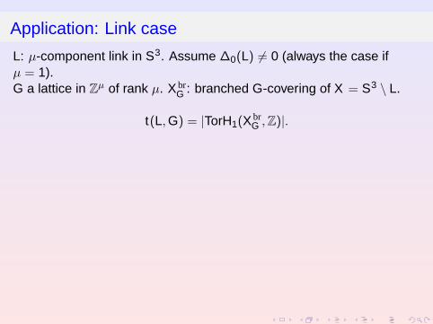
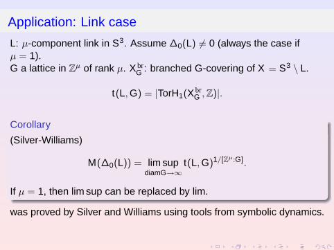
L: µ-component link in S3. Assume ∆0(L) 6= 0 (always the case ifµ = 1).G a lattice in Zµ of rank µ. X br
G : branched G-covering of X = S3 \ L.
t(L, G) = |TorH1(XbrG , Z)|.
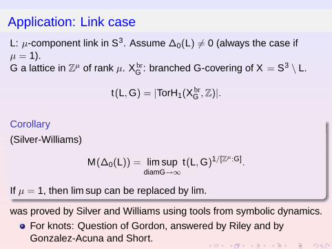
Corollary
(Silver-Williams)
M(∆0(L)) = lim supdiamG→∞
t(L, G)1/[Zµ:G].
If µ = 1, then lim sup can be replaced by lim.
was proved by Silver and Williams using tools from symbolic dynamics.
For knots: Question of Gordon, answered by Riley and byGonzalez-Acuna and Short.
Application: Link case
L: µ-component link in S3. Assume ∆0(L) 6= 0 (always the case ifµ = 1).G a lattice in Zµ of rank µ. X br
G : branched G-covering of X = S3 \ L.
t(L, G) = |TorH1(XbrG , Z)|.
Corollary
(Silver-Williams)
M(∆0(L)) = lim supdiamG→∞
t(L, G)1/[Zµ:G].
If µ = 1, then lim sup can be replaced by lim.
was proved by Silver and Williams using tools from symbolic dynamics.
For knots: Question of Gordon, answered by Riley and byGonzalez-Acuna and Short.

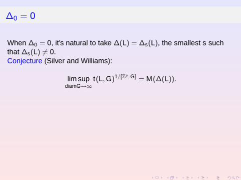
∆0 = 0
When ∆0 = 0, it’s natural to take ∆(L) = ∆s(L), the smallest s suchthat ∆s(L) 6= 0.
Conjecture (Silver and Williams):
lim supdiamG→∞
t(L, G)1/[Zµ:G] = M(∆(L)).
Proposition
lim supdiamG→∞
t(L, G)1/[Zµ:G] ≥ M(∆(L)).
Used a theorem of Schinzel-Bombieri-Zannier (2000) on co-primenessof specializations of multivariable polynomials.
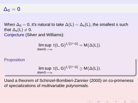
∆0 = 0
When ∆0 = 0, it’s natural to take ∆(L) = ∆s(L), the smallest s suchthat ∆s(L) 6= 0.Conjecture (Silver and Williams):
lim supdiamG→∞
t(L, G)1/[Zµ:G] = M(∆(L)).
Proposition
lim supdiamG→∞
t(L, G)1/[Zµ:G] ≥ M(∆(L)).
Used a theorem of Schinzel-Bombieri-Zannier (2000) on co-primenessof specializations of multivariable polynomials.
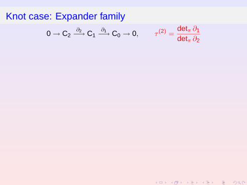
Knot case: Expander family
0 → C2∂2−→ C1
∂1−→ C0 → 0, τ (2) =detπ ∂1
detπ ∂2
One can prove the volume conjecture
exp(Vol(K )) = lim supdiamG→∞
t(K , G)1/[π:G]
if one can approximate both detπ ∂1, detπ ∂2 by finite quotients.
A convergence criterion of Luck: For A ∈ Mat(m× n, Z[π]), B = A∗A , ifthe eigenvalues of the BG near 0 “behaves well”, then
detπA = limG→∞
detπ/G AG.
For expander family, requirements of Luck criterion are satisfiedtrivially for A = ∂1:∂1 can be approximated by finite quotients (from expander family).
Same for ∂2? Yes =⇒ ‘volume conjecture” for hyperbolic knots.

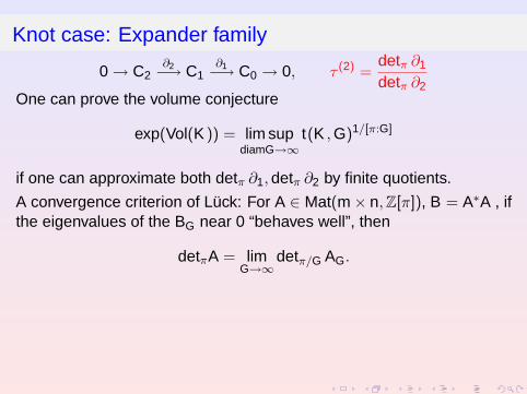
Knot case: Expander family
0 → C2∂2−→ C1
∂1−→ C0 → 0, τ (2) =detπ ∂1
detπ ∂2One can prove the volume conjecture
exp(Vol(K )) = lim supdiamG→∞
t(K , G)1/[π:G]
if one can approximate both detπ ∂1, detπ ∂2 by finite quotients.
A convergence criterion of Luck: For A ∈ Mat(m× n, Z[π]), B = A∗A , ifthe eigenvalues of the BG near 0 “behaves well”, then
detπA = limG→∞
detπ/G AG.
For expander family, requirements of Luck criterion are satisfiedtrivially for A = ∂1:∂1 can be approximated by finite quotients (from expander family).
Same for ∂2? Yes =⇒ ‘volume conjecture” for hyperbolic knots.

THANK YOU!