Topological abelian groups and equivariant homology

Marcelo A. Aguilar & Carlos Prieto∗

Instituto de Matematicas, UNAM, 04510 Mexico, D.F., Mexico

Email: marcelo@math.unam.mx, cprieto@math.unam.mx

Abstract We prove an equivariant version of the Dold-Thom theorem bygiving an explicit isomorphism between Bredon-Illman homology HG

∗(X ;L)

and equivariant homotopical homology π∗(FG(X,L)), where G is a finite

group and L is a G-module. We use the homotopical definition to obtainseveral properties of this theory and we do some calculations.

AMS Classification 55N91; 55P91,14F43

Keywords Equivariant homology, equivariant homotopy, coefficient sys-tems

0 Introduction

The presentation of homology using the Dold-Thom construction has been veryuseful in algebraic geometry. Lawson homology (see [14, 15, 9, 10]) was definedusing this approach. In this paper we study the Dold-Thom-McCord theorem(see [19]) in the equivariant case.

Let G be a finite group. If L is a G-module, then one can define a coefficientsystem L on the category of canonical orbits of G by L(G/H) = LH , where LH

is the subgroup of fixed points of L under H ⊂ G. One then has an ordinaryequivariant homology theory HG

∗ (−;L), called Bredon-Illman homology, whoseassociated coefficient system is precisely L. Let X be a (pointed) G-space andlet F (X,L) be the topological abelian group generated by the points of X , withcoefficients in L. Consider the subgroup FG(X,L) of equivariant elements, thatis, the elements

∑lxx in F (X,L) such that lgx = g · lx . Then one can associate

to X the homotopy groups πq(FG(X,L)), and one has that, if X is a G-

CW-complex, then HGq (X;L) is isomorphic to πq(F

G(X,L)). When G is the

trivial group, HG∗ (−;L) is singular homology and this statement is the classical

Dold-Thom theorem [7], which was extended to the equivariant case by Lima-Filho [16] (when L = Z with trivial G-action) and by dos Santos [21] (when

∗Corresponding author, Phone: ++5255-56224489, Fax ++5255-56160348. This au-thor was partially supported by PAPIIT grant IN110902 and by CONACYT grant43724.

1

L is any G-module). Both the original result and its equivariant generalizationwere proved by showing that the homotopical definition satisfies the axioms ofan ordinary or an equivariant homology theory, and then using a uniquenesstheorem for homology theories.

In this paper, we prove the equivariant Dold-Thom theorem by giving an explicitisomorphism HG

q (X;L) −→ πq(FG(X,L)) for all q and any X of the homotopy

type of a G-CW-complex (Theorem 1.2). This isomorphism is constructed inSection 2 in two steps as follows. Let F (S∗(X), L) be the (reduced) singularchain complex of X with coefficients in the G-module L. Since X is a G-space,we have an action of G on the singular simplexes of X , which we denote byσ 7→ g · σ . Let FG(S∗(X), L) be the subcomplex of equivariant chains, that is,chains

∑lσσ such that lg·σ = g · lσ . Using the theory of simplicial sets, we give

an isomorphism between the homology of this chain complex H∗(FG(S∗(X), L))

and π∗(FG(X,L)). Then we show that both the chain complex F G(S∗(X), L)

and Illman’s chain complex (see Section 2), which defines HG∗ (X;L) have the

same universal property (Propositions 2.10 and 2.11) so that they are canon-ically isomorphic. For a different approach to the nonequivariant Dold-Thomtheorem due to Friedlander and Mazur see [11].

In Section 1, we state the main theorem and prove that the theory HG∗ (X;L) =

π∗(FG(X,L)) is additive. In Section 3 we study the theory HG

∗ (X;L) in the gen-eral context of equivariant homology theories and coefficient systems. To eachequivariant homology theory hG∗ (−) one can associate the G-module hG0 (G).We show (Theorem 3.5) that there is an isomorphism between the group of nat-ural transformations Nat(hG∗ ,H

G∗ (−;L)) , and the group of G-homomorphisms

HomG(hG0 (G), L). We also show an analogous result for the classical equivarianthomology theory of Eilenberg and Steenrod.

Finally, in Section 4 we show that there is some interesting information inthe groups HG

0 (X;L), and using the transfer for ramified covering maps, wecalculate HZ2

q (X;L) for some Z2 -spaces X .

In this paper we shall work in the category of compactly generated weak Haus-

dorff spaces (see e.g. [18]).

1 Equivariant McCord’s topological groups

and equivariant homology

In [19], for a pointed topological space X and an abelian group L, McCordintroduced topological groups F (X,L) consisting of functions u : X −→ L

2

such that u(∗) = 0 and u(x) = 0 for all but a finite number of elements x ∈ X(see [1] for further details). If G is a finite group that acts continuously on Xleaving the base point fixed, and additively on L (on the left), then F (X,L)has a natural (left) action of G given by defining (g · u)(x) = gu(g−1x). Thisturns F (X,L) into a topological Z[G]-module.

Definition 1.1 Let G be a finite group, X a pointed G-space, and L a Z[G]-module. Define

FG(X,L) = {u ∈ F (X,L) | u(gx) = gu(x) for all x ∈ X, g ∈ G} .

In other words, FG(X,L) consists of the functions u ∈ F (X,L) that are G-functions, and coincides with the subspace F (X,L)G of fixed points under theG-action on F (X,L) given above.

Given a Z[G]-module L, there is a covariant coefficient system L called thesystem of invariants of L, which is given by taking the fixed point subgroupsLH of L under all subgroups H ⊂ G (see 3.2 3 below).

If X is a pointed G-space, then we denote by Sq(X) the set of singular q -simplexes in X , which has an obvious G-action. We may define a chain complexby taking as q -chains the elements of FG(Sq(X), L) (here Sq(X) is taken withthe discrete topology; see next section). The boundary operator is given asthe restriction of the boundary operator of the singular chain complex of X .We show below (Theorem 2.9) that this chain complex is naturally isomorphicto Illman’s chain complex [13], which defines the Bredon-Illman equivarianthomology of X with coefficients in L, HG

q (X;L).

The main theorem of the paper is the following.

Theorem 1.2 Let X be a pointed G-space of the same homotopy type of a

G-CW-complex. Then there is an isomorphism HGq (X;L) −→ πq(F

G(X,L))given by sending a homology class [u] represented by a cycle u =

∑lσσ all

of whose faces are zero, to the map u : (∆q, ∆q) −→ (FG(X,L), ∗) such that

u(t) =∑lσσ(t).

In particular, when G is the trivial group and L = Z, this will give a new proofof the classical Dold-Thom theorem, since SP∞X ≈ F (X,N) ' F (X,Z).

Definition 1.3 Define the (reduced) equivariant homology theory HG∗ with

coefficients in the coefficient system L by

HGq (X;L) = πq(F

G(X,L)) .

3

As usual, HGq (X;L) = HG

q (X+;L), where X+ = X t {∗} has the obviousextended action.

We devote the next section to the proof of Theorem 1.2. Meanwhile, we makesome further considerations on our equivariant homology groups.

We shall now prove that our equivariant homology theory HG∗ is additive. To

prove that, we need the following concept. Let Xα , α ∈ Λ, be a family ofpointed G-spaces and let L be a Z[G]-module. Then we have (algebraically)the direct sum F =

⊕α∈Λ F

G(Xα, L). In order to furnish it with a convenienttopology, take

F n = {(uα) ∈ F | #{α ∈ Λ | uα 6= 0} ≤ n} .

Then obviously F n ⊂ F n+1 , and⋃n F

n = F . For each n, there is a surjection∐

α1,...,αn∈Λ

(Xα1 × L) × · · · × (Xαn × L) � F n .

Furnish F n with the identification topology and F with the topology of theunion of the F ns. One clearly has the following.

Lemma 1.4 There is an isomorphism of topological groups⊕

α∈Λ

FG(Xα, L) ∼= FG(∨

α∈Λ

Xα, L))

induced by the inclusions Xα ↪→∨Xα .

Proof: The inverse is given by the restrictions F G(∨Xα, L) −→ FG(Xα, L),

u 7→ u|Xα .

Since obviously πq(⊕

α FG(Xα, L)) ∼=

⊕α πq(F

G(Xα, L)), as a consequence,we have the next.

Theorem 1.5 There is an isomorphism HGq (∨αXα;L) ∼=

⊕α HG

q (Xα;L).

A more general case is as follows.

Definition 1.6 A G-space X is said to be G-0-connected (or G-path con-

nected), if given any two points x, y ∈ X , then there exists a G-path (σ, g) :x 'G y , that is, an element g ∈ G and an ordinary path σ from x to gy . Therelation 'G is clearly an equivalence relation, and the equivalence classes arecalled the G-path components of X (see [20]).

4

Assume that a G-space X is locally 0-connected, then, since every G-pathcomponent Xα of X is a topological sum of ordinary path components, there isa decomposition X =

∐αXα . Given that (

∐αXα)

+ =∨αX

+α , a consequence

of the additivity (1.4) is the following.

Corollary 1.7 Let X be a locally 0-connected G-space. There is an isomor-

phism HGq (X;L) ∼=

⊕α HG

q (Xα;L), where the G-spaces Xα denote the G-path

components of X .

2 Proof of the main theorem

In this section we prove Theorem 1.2. We use the techniques of simplicial setsfor this. As already mentioned, in particular, this will provide a new proof ofthe classical Dold-Thom theorem [7].

We denote by ∆ the category whose objects are the sets n = {0, 1, 2, . . . , n}and whose morphisms f ∈ ∆(m,n) are monotonic functions f : m −→ n.Recall that a simplicial set is a contravariant functor K : ∆ −→ Set; we denotethe set K(n) simply by Kn . Let ∆[q] be the simplicial set ∆[q]n = ∆(−, q).We write |K| for the geometrical realization given by

|K| =⊔

n

(Kn × ∆n)/∼ ,

where ∆n = {(t0, t1, . . . , tn) ∈ Rn+1 | ti ≥ 0, i = 0, 1, 2, . . . , n, t0 + t1 + · · · +tn = 1} is the standard n-simplex, and the equivalence relation is given by(fK(σ), t) ∼ (σ, f#(t)), σ ∈ Kn , t ∈ ∆m . Here f# denotes the map affinelyinduced by f in the standard simplices. Denote the elements of |K| by [σ, t],σ ∈ Kn and t ∈ ∆n .

We say that a simplicial set K is pointed, if it is provided with a morphism(natural transformation) ∆[0] −→ K . This means that each set Kn has a basepoint and that for each f : m −→ n, the induced function fK : Kn −→ Km isbase-point preserving.

Definition 2.1 Given a pointed simplicial set K and an abelian group L, wedefine the simplicial abelian group F (K,L) by F (K,L)n = F (Kn, L) (as men-tioned in Section 1, where Kn has the discrete topology). The homomorphisminduced by f : m −→ n is fK∗ : F (Kn, L) −→ F (Km, L).

The proof of the following uses results of Milnor (see [17]).

5

Lemma 2.2 The geometric realization |F (K,L)| is an abelian topological

group such that [v, t] + [v′, t] = [v + v′, t].

Proof: Consider the projections pi : F (K,L)×F (K,L) −→ F (K,L), i = 1, 2,and the induced maps |pi| : |F (K,L) × F (K,L)| −→ |F (K,L)|, and defineη : |F (K,L) × F (K,L)| −→ |F (K,L)| × |F (K,L)| by

η[(v, v′), t] = (|p1|[(v, v′), t], |p2|[(v, v

′), t])

= ([p1(v, v′), t], [p2(v, v

′), t])

= ([v, t], [v′, t]) .

By [17, 14.3], η is a homeomorphism. The group structure + in |F (K,L)| isthen given by the diagram

|F (K,L)| × |F (K,L)|η−1

//

+ **UUUUUUUUUUUUUUUU|F (K,L) × F (K,L)|

|µ|��

|F (K,L)| ,

where µ : F (K,L)×F (K,L) −→ F (K,L) is the simplicial group structure.

Proposition 2.3 The topological groups F (|K|, L)| and |F (K,L)| are natu-

rally isomorphic.

Proof: Takeϕ : F (|K|, L) −→ |F (K,L)|

given by

ϕ(u) =∑

[σ,t]∈|K|

[u[σ, t]σ, t] ,

where u : |K| −→ L, σ ∈ Kn , and t ∈ ∆n (thus u[σ, t]σ ∈ F (Kn, L)). UsingLemma 2.2 one shows that ϕ is a homomorphism. Thus we only need to checkthat ϕ|Fk(|K|,L) is continuous. Consider the diagram

(L× |K|)k //______

��

|F (K,L)|k

sum

��Fk(|K|, L)

ϕ|Fk(|K|,L)

// |F (K,L)| ,

where the map on the top is the product of the maps given by the next diagram.

L× (⊔n(Kn × ∆n) //___

��

⊔n(F (Kn, L) × ∆n

��L× |K| // F (|K|, L) ,

6

where the top map is given by (l, σ, t) 7→ (lσ, t).

To see that ϕ is an isomorphism of topological groups, we define its inverseψ : |F (K,L)| −→ F (|K|, L) as follows. Take v ∈ F (Kn, L); then ψ[v, t] =∑

σ∈Knv(σ[σ, t]. To see that ψ is well defined, take v =

∑ri=1 liσi ; then fK∗ (v) =∑r

i=1 lifK(σi). Thus

ψ[fK∗ (v), t] =

r∑

i=1

[fK(σi), t] =

r∑

i=1

[σi, f#(t)] = ψ[v, f#(t)] .

To see that ψ is continuous, consider the diagram⊔n(F (Kn, L) × ∆n //___

��

SP∞F (|K|, L)

sum

��|F (K,L)|

ψ// F (|K|, L) ,

where the top arrow given by (∑

i li, σi), t) 7→ 〈l1[σ1, t], . . . 〉 is obviously con-tinuous.

Moreover, ψ is a homomorphism. Namely, given [v, t], [v ′, t′] ∈ |F (K,L)|, byLemma 2.2, there exist unique elements, w,w′, t′′ such that [v, t] = [w, t′′],[v′, t′] = [w′, t′′]. Thus

ψ([v, t] + [v′, t′] = ψ([w, t′′] + [w′, t′′])

= ψ[w + w′, t′′]

=∑

σ

(w +w′)(σ)[σ, t′′]

= ψ[w, t′′] + ψ[w′, t′′] = ψ[v, t] + ψ[v′, t′] .

In generators, we have that ψϕ(l[σ, t]) = ψ[lσ, t] = l[σ, t], thus ψ◦ϕ is the iden-tity. On the other hand, ϕψ[v, t] = ϕ(

∑σ∈Kn

v(σ[σ, t]) =∑

σ∈Kn[v(σ)σ, t] =

[∑

σ∈Knv(σ)σ, t] = [v, t], where the next to the last equality follows by Lemma

2.2.

Definition 2.4 Let G be a finite group. A (pointed) G-simplicial set is a(pointed) simplicial set K such that G acts on each Kn and the action of everyg ∈ G determines a (pointed) isomorphism of K . In other words, it is a functorK : ∆ −→ G-Set∗ .

Given a pointed G-simplicial set K and a Z[G]-module L, then F (K,L) inher-its an action of G, as also do |K|, F (|K|, L), and |F (K,L)|. By the naturalityof the isomorphism of Proposition 2.3 we obtain the following.

7

Corollary 2.5 Let K be a G-simplicial set. Then the topological groups

F (|K|, L) and |F (K,L)| are G-isomorphic.

Let K be a G-simplicial set and H ⊂ G be a subgroup. Define KH as thesimplicial set such that (KH)n = (Kn)

H (write this set as KHn ). Then KH

is a simplicial subset of K and one easily verifies that |KH | = |K|H and|FH(K,L)| = |F (K,L)|H . Thus we have the following.

Corollary 2.6 Let K be a G-simplicial set. Then the topological groups

FH(|K|, L), |F (K,L)|H , and |FH(K,L)| are isomorphic.

Let A be a simplicial abelian group. Recall that the q -homotopy group of A isdefined by

πq(A) = Hq(N(A), ∂) ,

where N(A)q = Aq ∩ ker d0 ∩ · · · ∩ ker dq−1 and ∂q = (−1)qdq ; here di is theith face operator of A. On the other hand, A can be seen as a chain complex,with ∂ : Aq −→ Aq−1 given by

∑qi=0(−1)idi .

We have the following result (cf. [17, 22.1]).

Proposition 2.7 The canonical inclusion of chain complexes N(A) ↪→ A in-

duces an isomorphism in homology.

Proof: The chain complex A is filtered by chain complexes Ap , where

Apq = {u ∈ Aq | di(u) = 0, 0 ≤ i < min{q, p}} .

The canonical inclusion ip : Ap+1 ↪→ A

p is a chain homotopy equivalence withinverse rp : A

p −→ Ap+1 given by rp(u) = u − spdp(u), where sp is the pth

degeneracy operator of A. Obviously, rp◦ ip = 1Ap+1 ; conversely, ip ◦rp is chainhomotopic to 1Ap via the chain homotopy hp : A

pq −→ A

pq+1 given by

hp(u) =

{0 if q < p

(−1)psp(u) if q ≥ p .

Let G be a finite group and X a pointed G-space and let S(X) denote thesingular simplicial set given for each q by

Sq(X) = {σ : ∆q −→ X | σ is a map} .

8

Then, in fact, S(X) is a pointed simplicial G-set with the usual simplicialstructure. On the other hand, let T

Gq (X) be the G-singular set given by

TGq (X) = {T : ∆q ×G/H −→ X | T is an equivariant map and H ⊂ G} ,

q ∈ N (here ∆q has trivial G-action).

Let L be a Z[G]-module. Define F (TGq (X), L) = {v : TGq (X)+ −→ L | v ∈

F (TGq (X)+, L), v(T ) ∈ LH if T : ∆q×G/H −→ X}. One easily sees that these

groups are exactly Illman’s groups CGq (X;L) ([13, Def. 3.3]). As Illman does, wemay declare that the generator lT is related to l′T ′ if there exists a G-functionα : G/H −→ G/H ′ such that the following diagram commutes

∆q ×G/H

T %%JJJJJJJJJJ

id×α // ∆q ×G/H ′

T ′yyssssssssss

X

and l′ = α∗(l) ∈ LH′

(see 3.2 3. below). Divide the group F (TGq (X), L) bythe subgroup generated by the differences lT − l′T ′ where either lT is relatedto l′T ′ or l′T ′ is related to lT , as well as by all elements lT such that T :∆q×G/H −→ X is constant with value the base point x0 , to obtain the groupF ′(TGq (X), L). The following is clear.

Proposition 2.8 The simplicial group FG(S(X), L) and the graded group

F ′(TG(X), L) are chain complexes.

In fact, the chain complex F ′(TG(X), L) is identical to Illman’s chain complexSG(X,x0;L) (cf. [13, p. 15]). Then we have the following.

Theorem 2.9 The chain complexes F ′(TG(X), L) and FG(S(X), L) are iso-

morphic.

The proof of this theorem requires some preparation.

Let S be a pointed G-set with G-fixed base point σ0 . For each σ ∈ S , let µσ :LGσ −→ FG(S,L) be given by µσ(l) =

∑ni=1(gil)(giσ), where {[g1], . . . [gn]} =

G/Gσ . Then µσ0 = 0 and µσ = µgσ ◦ λg , where λg(l) = gl .

We have the following universal property of FG(S,L).

9

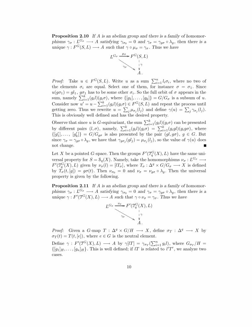
Proposition 2.10 If A is an abelian group and there is a family of homomor-

phisms γσ : LGσ −→ A satisfying γσ0 = 0 and γσ = γgσ ◦ λg , then there is a

unique γ : FG(S,L) −→ A such that γ ◦ µσ = γσ . Thus we have

LGσµσ //

γσ%%JJJJJJJJJJ

FG(S,L)

γ

����

�

A .

Proof: Take u ∈ FG(S,L). Write u as a sum∑n

i=1 liσi , where no two ofthe elements σi are equal. Select one of them, for instance σ = σ1 . Sinceu(gσ1) = gl1 , gσ1 has to be some other σi . So the full orbit of σ appears in thesum, namely

∑ki=1(gil)(giσ), where {[g1], . . . , [gk]} = G/Gσ is a subsum of u.

Consider now u′ = u−∑k

i=1(gil)(giσ) ∈ FG(S,L) and repeat the process untilgetting zero. Thus we rewrite u =

∑j µσj

(lj) and define γ(u) =∑

j γσj(lj).

This is obviously well defined and has the desired property.

Observe that since u is G-equivariant, the sum∑k

i=1(gil)(giσ) can be presented

by different pairs (l, σ), namely,∑k

i=1(gil)(giσ) =∑k

i=1(gigl)(gigσ), where{[g′1], . . . , [g′k]} = G/Ggσ is also presented by the pair (gl, gσ), g ∈ G. Butsince γσ = γgσ ◦ λg , we have that γgσj

(glj) = µσj(lj), so the value of γ(u) does

not change.

Let X be a pointed G-space. Then the groups F ′(TGq (X), L) have the same uni-

versal property for S = Sq(X). Namely, take the homomorphisms νσ : LGσ −→F ′(TGq (X), L) given by νσ(l) = [lTσ], where Tσ : ∆q ×G/Gσ −→ X is definedby Tσ(t, [g]) = gσ(t). Then νσ0 = 0 and νσ = νgσ ◦ λg . Then the universalproperty is given by the following.

Proposition 2.11 If A is an abelian group and there is a family of homomor-

phisms γσ : LGσ −→ A satisfying γσ0 = 0 and γσ = γgσ ◦ λg , then there is a

unique γ : F ′(TG(X), L) −→ A such that γ ◦ νσ = γσ . Thus we have

LGσνσ //

γσ&&MMMMMMMMMMMM

F ′(TGq (X), L)

γ

����

�

A .

Proof: Given a G-map T : ∆q × G/H −→ X , define σT : ∆q −→ X byσT (t) = T (t, [e]), where e ∈ G is the neutral element.

Define γ : F ′(TG(X), L) −→ A by γ[lT ] = γσT(∑n

i=1 gil), where GσT/H =

{[g1]H , . . . , [gn]H}. This is well defined; if lT is related to l′T ′ , we analyze twocases.

10

We assume first that H ⊂ H ′ and that α : G/H −→ G/H ′ is the quotientmap. Then T ′ ◦ (id×α) = T , thus T (t, [g]H) = T ′(t, [g]H′), and l′ = α∗(l) =∑r

j=1 h′jl , where H ′/H = {[h′1]H , . . . , [h

′r]H}. Notice that therefore σT ′ = σT ,

so that we have H ⊂ H ′ ⊂ GσT. Let GσT

/H ′ = {[g′1]H′ , . . . , [g′m]H′}. Therefore,GσT

/H = g′1(H′/H) ∪ · · · ∪ g′m(H ′/H). Hence

γ[lT ] = γσT

r∑

j=1

(g′1h′jl) + · · · +

r∑

j=1

(g′mh′jl)

On the other hand,

γ[l′T ′] = γσT

(m∑

i=1

(g′il′)

),

but l′ =∑r

i=1 h′il . Thus γ[lT ] = γ[l′T ′].

Now assume that H ′ = g−10 Hg0 and α = ρg0 : G/H −→ G/H ′ is given by

right translation with g0 . Then α∗ : LH −→ LH′

is given by left translationwith g−1

0 , namely α∗(l) = g−10 l . Hence l′ = g−1

0 l and σT ′ = g−10 σT . Moreover,

GσT ′ = g−10 GσT

g0 . Thus, if GσT/H = {[g1]H , . . . , [gn]H}, then GσT ′ /H

′ =

{[g−10 g1g0]H′ , . . . , [g−1

0 gng0]H′}, and so

γ[l′T ′] = γσT ′

(n∑

i=1

g−10 gig0l

′

)= γg−1

0 σT

(n∑

i=1

g−10 gil

)

= γσTg0

(n∑

i=1

g−10 gil

)= γσT

(n∑

i=1

gil

)= γ[lT ] .

Obviously, γ has the desired properties.

Proof of Theorem 2.9: The isomorphism F ′(TGq (X), L) −→ FG(Sq(X), L) in theprevious corollary, as provided by the universal property, is given by

[lT ] 7−→

n∑

i=1

(gil)(giσT ) ,

where T : ∆q × G/H −→ X , l ∈ LH , and G/H = {[g1]H , . . . , [gn]H}. Oneeasily verifies that this is a chain map.

The following proposition is a generalization to the equivariant case of a theoremof Milnor (see [17, 16.6]).

11

Proposition 2.12 Let X be a pointed G-space of the same homotopy type

of a G-CW-complex. Then ρ : |S(X)| −→ X given by ρ[σ, t] = σ(t) is a G-

homotopy equivalence.

Proof: Let H ⊂ G be any subgroup. Note first, as already mentioned before,that the identity induces a homeomorphism |KH | ≈ |K|H for any simplicial G-set K . On the other hand, one also has a canonical isomorphism of simplicialsets S(XH ) ∼= S(X)H . We have that Milnor’s map ρ : |S(X)| −→ X , beingnatural, is a G-map. On the other hand, again by the naturality, it restricts toρH : |S(XH )| −→ XH , which by a theorem of Milnor is a homotopy equivalence.Therefore, one has the following commutative triangle

|S(X)|HρH

// XH

|S(XH)|

≈

OO

ρH

;;vvvvvvvvv

where the vertical arrow is a homeomorphism, as mentioned above. Hence, ρH

is a homotopy equivalence for every H ⊂ G. By a result of Bredon [4, II(5.5)],then ρ is a G-homotopy equivalence.

Proof of Theorem 1.2: We shall give an isomorphism

HG(X;L) ∼= Hq(FG(Sq(X), L)) −→ πq(F

G(X,L)) = HGq (X;L) .

Here the left-hand side is the Bredon-Illman (reduced) homology of X , and thefirst isomorphism follows from the natural isomorphism of Theorem 2.9.

To construct the arrow, we shall give several isomorphisms as depicted in thefollowing diagram, where H ⊂ G is any subgroup.

Hq(FH(S(X), L)) oo i∗

∼=

����

�πq(F

H(S(X), L))Ψ∼=

// πq(S(|FH (S(X), L)|))

Φ∼=��

πq(FH(X,L)) oo

∼=ρ∗

πq(FH(|S(X)|, L)) oo

∼=

ψ∗πq(|F

H(S(X), L)|)

By Proposition 2.7, i∗ is an isomorphism. In particular, this shows that everycycle in HG(X;L) is represented by a chain u, all of whose faces are zero. Weshall call this a special chain.

The homomorphism Ψ, which is given by Ψ(u)[t] = [u, t], where u is a specialq -chain and t ∈ ∆q , is an isomorphism, as follows from [17, 16.6].

12

In order to define Φ, we must express Ψ(u) as a map γ : (∆[q], ∆[q]) −→(S|FH (S(X), L)|, ∗). By the Yoneda lemma, γ is the unique map such thatγ(δq) = Ψ(u), where δq = id : q −→ q . The homomorphism Φ, defined byΦ[γ][f, s] = γ(f)(s), for f ∈ ∆[q]n and s ∈ ∆n , is given by the adjunctionbetween the realization functor and the singular complex functor (see [17, 16.1]).

That ψ∗ is an isomorphism follows from Proposition 2.3. Finally, the homomor-phism ρ∗ is an isomorphism by 2.12.

Chasing along this diagram and using the homeomorphism |∆[q]| −→ ∆q givenby [f, t] 7→ f#(t), one obtains that the isomorphism maps a homology class[u] ∈ Hq(F

H(S(X), L)) represented by a special chain u =∑

σ lσσ , to the mapu : (∆q, ∆q) −→ (FH(X,L), ∗) given by u(t) =

∑lσσ(t).

3 Equivariant homology and other coefficient systems

In this section we recall the general concept of a (covariant) coefficient systemfor a group G and give explicit examples of ordinary equivariant homologytheories with particular systems as coefficients.

Definition 3.1 Let G be a finite group. A covariant coefficient system forG, M , is a covariant functor from the category of homogeneous sets G/H ,H a subgroup of G, and G-functions α : G/H −→ G/K , to the category ofabelian groups. We denote the induced homomorphisms by α∗ : M(G/H) −→M(G/K). There is, of course, a category CoeffsysG of covariant coefficientsystems for G.

Examples 3.2 Let L be a Z[G]-module. We have the following associatedcovariant coefficient systems.

1. To start with, consider the constant coefficient system, denoted again byL, with value the group L given by L(G/H) = L for all H ⊂ G and forα : G/H −→ G/K , H ⊂ K ⊂ G, by α∗ = 1L . This is realized by thetheory

hGq (X;L) = Hq(X/G;L) ,

where the second term is singular homology with coefficients in L.

2. Another useful example is the following. Let L be given by definingL(G/H) = LH , the quotient of L by the subgroup generated by theelements of the form l − h · l , l ∈ L, h ∈ H , and for a : G/H −→ G/K ,a∗ : LH −→ LK is the quotient homomorphism. We call it the system of

13

coinvariants of L. If, in particular, L has trivial action, then this coeffi-cient system coincides with the constant system given in 1. The coefficientsystem L is realized by a theory constructed by Eilenberg and Steenrod[8] (see also [6]) as follows. Consider the usual singular complex S∗(X)on which G acts (here G acts on X on the right). Take the complexS∗(X) ⊗Z[G] L. Define the classical ordinary equivariant homology theory

by

HGq (X;L) = Hq(S∗(X) ⊗Z[G] L) .

If X = G/H , then HGq (G/H;L) = 0 if q > 0 and H

G0 (G/H;L) =

S0(G/H) ⊗Z[G] L = Z[G/H] ⊗Z[G] L ∼= LH .

3. The other example that we consider is L, that we call the system ofinvariants of L.† It is defined as follows. Take L(G/H) = LH = {l ∈L | h · l = l for all h ∈ H}. For H ⊂ K ⊂ G and α : G/H −→ G/Kthe quotient function, take α∗(l) =

∑k∈[K/H] kl , where [K/H] denotes a

set of representatives in K of the cosets of H in K . For any equivariantmap α : G/H −→ G/K one has that H ⊂ aK = aKa−1 for some a ∈ G,and so α is the composite of the quotient map G/H −→ G/aK and theobvious bijection G/aK ≈ G/K . Hence we define a∗ : LH −→ LK asthe composite of LH −→ L

aK given by l 7→∑

k∈[aK/H] kl followed by

the isomorphism LaK −→ LK given by l 7→ a−1l . As shown in the main

theorem, our theory

HGq (X;L) = πq(F

G(X,L))

realizes L. Observe that if L has trivial G-action, then L defines thesemiconstant coefficient system, namely, L(G/H) = L for all H ⊂ G andfor α : G/H −→ G/K , define α∗ : L −→ L by α∗(l) = (|K|/|H|)l .

As shown in [12], the system of invariants is right adjoint to the forgetful func-tor from the category of coefficient systems to the category of Z[G]-modules.Similarly, one can show that the system of coinvariants is left adjoint to thesame forgetful functor. One has the following.

Proposition 3.3 There are natural bijections

CoeffsysG(L,M) ∼= HomG(L,M(G)) ,

CoeffsysG(M,L) ∼= HomG(M(G), L) .

†Notice that the system of invariants of L is denoted by L in [16] and [21].

14

As shown by Illman [13], given any (covariant) coefficient system, there is anordinary equivariant homology theory HG

∗ (−;M) with M as coefficients. More-over, given any natural transformation µ : M −→ N of coefficient systems,there is an extension of it to a natural transformation µ : HG

∗ (−;M) −→HG

∗ (−;N) of (ordinary) homology theories. On the other hand, Willson [22]constructs for any equivariant homology theory hG a (natural) spectral se-quence such that E2

p q∼= HG

p (X;hGq (·)), where hGq (·) is the coefficient system

given by G/H 7→ hGq (G/H), that converges to hGp+q(X). Clearly, if hG is or-

dinary, then this spectral sequence collapses. This shows that if µ : hG −→ kG

is a natural transformation of ordinary homology theories such that it inducesthe zero transformation in coefficients hG(·) −→ kG(·), then µ itself has to bezero. We thus have the following.

Proposition 3.4 There is an isomorphism between natural transformations of

coefficient systems and natural transformations of ordinary homology theories.

More precisely, we have

CoeffsysG(M,N) ∼= Nat(HG∗ (−;M),HG

∗ (−;N)) .

By this and the adjunction result 3.3 above, we have the following.

Theorem 3.5 There are isomorphisms

HomZ[G](L, hG0 (G)) ∼= Nat(HG

∗ (−;L), hG∗ ) ,

HomZ[G](hG0 (G), L) ∼= Nat(hG∗ ,H

G∗ (−;L)) ,

where hG∗ represents any ordinary equivariant homology theory, HG∗ (−;L) the

classical equivariant homology theory, and HG∗ (−;L) the homology theory that

we defined in 1.3.

4 Some computations of the equivariant homology groups

HG∗ (−; L)

In this section, we compute some equivariant homology groups, especially indimension 0, for the theory defined in 1.3.

Theorem 4.1 Let X be a 0-connected space with a free G-action, and let Lbe a Z[G]-module. Then

HG0 (X;L) ∼= LG ,

15

where LG = L/〈l−g · l〉 is the quotient of L divided by the subgroup generated

by the elements l − g · l , l ∈ L, g ∈ G.

Proof: First observe that if the G-action on L is trivial, then the transfer of

p : X −→ X/G yields an isomorphism tp : F (X/G+, L)∼=

−→ FG(X+, L) (see[2, Thm. 6.2]), that implies the result.

For the general case, let {xi} be a set of representatives in X of the orbits (inX/G), and define

εG : FG(X+, L) −→ LG by εG(u) =∑

i

u(xi) ,

where l ∈ LG denotes the class of l ∈ L. One easily verifies that εG is inde-pendent of the choice of the representatives xi . We shall show below that εG

is continuous, but for the time being, we assume it is.

Let α : L −→ FG(X+, L) be given by α(l) = lx0 , where

lx0(x) =

{g · l if x = gx0,

0 if x /∈ orbit(x0),

and x0 is one of the representatives of the orbits taken above. We then have acommutative diagram

L

��

α // FG(X+, L)

��LG α

//___ π0(FG(X+, L)) .

Namely, if we take h ∈ G, we have to prove that both lx0 and (hl)x0 lie

in the same path component of FG(X+, L). Clearly, (hl)x0 = ˜l(h−1x0). Letσ : I −→ X be a path from x0 to h−1x0 , and define σ : I −→ FG(X+, L) by

σ(t) = lσ(t). Then σ(0) = lx0 , and σ(1) = ˜l(h−1x0) = (hl)x0 .

In order to prove that σ is continuous, note first that lx =∑

g∈G(g · l)(gx),where

(lx)(x′) =

{l if x′ = x,

0 if x′ 6= x,

and t 7→ (g · l)(gσ(t)) is continuous because the action of G on X is continuous.Thus, σ is continuous and α is well defined.

Consider εGα(l) = εG[lx0] = l . Thus εG ◦ α = 1LGand hence α is injective.

16

To see that α is also surjective, take any u ∈ FG(X+, L) and call li = u(xi) for

each representative xi of the orbits in X . Then u =∑

i lixi and hence {lxi}, l ∈L, is a set of generators of FG(X+, L). Since α is obviously a homomorphism,

it is enough to show that every generator [lxi] of π0(FG(X+, L)) is in the image

of α. Let now σ : I −→ X be a path from x0 to xi , then σ(t) = lσ(t) is a path

from α(l) = lx0 to lxi .

To finish the proof we have to show that εG is indeed continuous. Let π : L −→LG be the quotient homomorphism and call q = p∗|FG(X+,L) : FG(X+, L) −→

F (X/G+, L). Take u ∈ FG(X+, L); then

(π∗q(u))[x] = π

∑

x′∈p−1[x]

u(x′)

= π

∑

g∈G

u(gx)

= π

∑

g∈G

g · u(x)

=∑

g∈G

π (g · u(x))

= |G|u(x),

hence the image of π∗ ◦ q lies in F (X/G+, |G|LG) where one can divide by|G|. Call γ∗ : F (X/G+, |G|LG) −→ F (X/G+, LG) the homomorphism given bydividing the values of the elements by |G|. Then εG is the composite

FG(X+, L)γ∗◦π∗◦q // F (X/G+, LG)

ε // LG ,

where ε : F (X/G+, LG) −→ LG is the augmentation given by

ε(v) =∑

x∈X/G

v(x) .

Since all maps in the composite are continuous, so is εG too.

Theorem 4.2 Let X be a G-0-connected G-space with a single orbit type

and let L have trivial G-action. Then HG0 (X;L) ∼= L.

Proof: The result follows from the same arguments of 4.1, but, on the onehand, since L has trivial G-action, G-paths are good enough, and on the other,instead of dividing by the order of G, we divide by the order of any orbit.

17

As a consequence of 1.7 and 4.2, we have the next result.

Corollary 4.3 Let X be a locally path-connected G-space and let Xα , α ∈ Λ,

be the G-path components of X such that each G-path component has a single

orbit type. Then

HG0 (X;L) ∼=

⊕

α∈Λ

Lα , Lα = L ∀α .

Remark 4.4 Call πG0 (Y ) the set of G-path connected components of the G-space Y . There is a canonical function πG0 (Y ) −→ π0(Y/G) which is obviouslysurjective. It is also injective. To see this one has to apply the Covering Homo-topy Theorem for orbit maps q : Y −→ Y/G of Palais (see [5, II.7.3]). Namely,let x and y be two points in Y such that q(x) and q(y) are connected in Y/Gby a path ω . Taking X = G in Palais’ theorem (in Bredon’s notation), thenω can be seen as a homotopy F ′ : X/G × I −→ Y/G. Taking f : X −→ Y tobe given by f(g) = gx, we have an equivariant map, so that the assumptionsof the theorem are fulfilled (then f ′ : X/G −→ Y/G chooses q(x)). Thus thereexists an equivariant homotopy F : X × I −→ Y starting at F and coveringF ′ , that is, by restricting F to {e}×I we have a path ω in Y starting at x andcovering ω . Hence, qω(1) = ω(1) = q(y), and so ω(1) = gy for some g ∈ G.This means that x and y are in the same G-path component of Y .

By the previous remark, it is the trivial G-homology theory hG∗ given byhG∗ (X;L) = H∗(X/G;L), the one that has the property that if X is locally 0-connected, then hG0 (X;L) ∼= ⊕πG

0 (X)L, L some abelian group with no G-action.That is, the trivial zero-G-homology groups measure the G-path-connectedness.In what follows we analyze the groups HG

0 (X;L) in some special cases.

Let X be a G-space with (at least) one fixed point x0 . The inclusion i : S0 ↪→X+ that sends one point to + and the other to x0 is an equivariant embeddingwhose image is a retract with the obvious retraction r : X+ −→ S0 . Thuswe have that r∗ : FG(X+, L) −→ F (S0, L) = L is a split epimorphism. ThusFG(X+, L) ∼= L× ker r∗ . Thus we have the following.

Proposition 4.5 Let X be a G-space with a fixed point x0 under the G-

action, and let L have a trivial G-action. Then HG0 (X;L) ∼= L × π0(ker r∗).

18

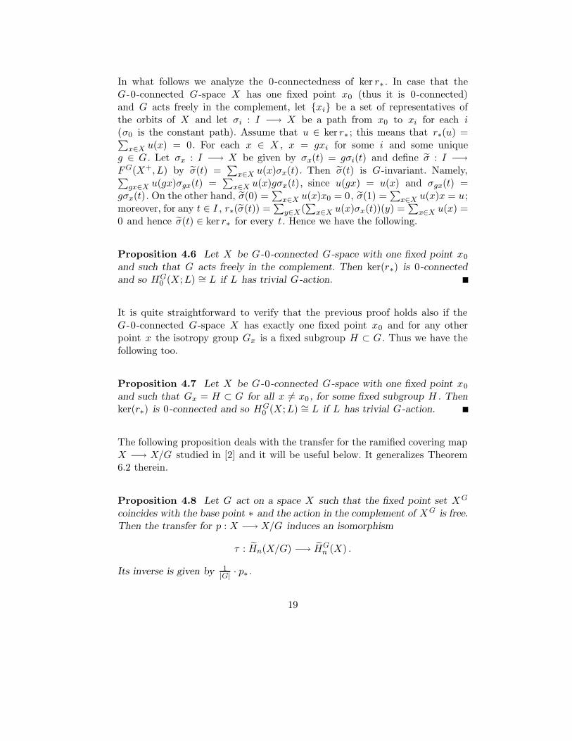
In what follows we analyze the 0-connectedness of ker r∗ . In case that theG-0-connected G-space X has one fixed point x0 (thus it is 0-connected)and G acts freely in the complement, let {xi} be a set of representatives ofthe orbits of X and let σi : I −→ X be a path from x0 to xi for each i(σ0 is the constant path). Assume that u ∈ ker r∗ ; this means that r∗(u) =∑

x∈X u(x) = 0. For each x ∈ X , x = gxi for some i and some uniqueg ∈ G. Let σx : I −→ X be given by σx(t) = gσi(t) and define σ : I −→FG(X+, L) by σ(t) =

∑x∈X u(x)σx(t). Then σ(t) is G-invariant. Namely,∑

gx∈X u(gx)σgx(t) =∑

x∈X u(x)gσx(t), since u(gx) = u(x) and σgx(t) =gσx(t). On the other hand, σ(0) =

∑x∈X u(x)x0 = 0, σ(1) =

∑x∈X u(x)x = u;

moreover, for any t ∈ I , r∗(σ(t)) =∑

y∈X(∑

x∈X u(x)σx(t))(y) =∑

x∈X u(x) =0 and hence σ(t) ∈ ker r∗ for every t. Hence we have the following.

Proposition 4.6 Let X be G-0-connected G-space with one fixed point x0

and such that G acts freely in the complement. Then ker(r∗) is 0-connected

and so HG0 (X;L) ∼= L if L has trivial G-action.

It is quite straightforward to verify that the previous proof holds also if theG-0-connected G-space X has exactly one fixed point x0 and for any otherpoint x the isotropy group Gx is a fixed subgroup H ⊂ G. Thus we have thefollowing too.

Proposition 4.7 Let X be G-0-connected G-space with one fixed point x0

and such that Gx = H ⊂ G for all x 6= x0 , for some fixed subgroup H . Then

ker(r∗) is 0-connected and so HG0 (X;L) ∼= L if L has trivial G-action.

The following proposition deals with the transfer for the ramified covering mapX −→ X/G studied in [2] and it will be useful below. It generalizes Theorem6.2 therein.

Proposition 4.8 Let G act on a space X such that the fixed point set XG

coincides with the base point ∗ and the action in the complement of XG is free.

Then the transfer for p : X −→ X/G induces an isomorphism

τ : Hn(X/G) −→ HGn (X) .

Its inverse is given by 1|G| · p∗ .

19

Proof: In the McCord topological groups F (X/G,Z) and F G(X,Z) everyelement is zero in the base point. Thus in the diagram

Xp //

u��?

????

???

X/G

u}}{{{{

{{{{

Z

where u is G-invariant, u exists if and only if u exists. Since off the fixed point∗ the multiplicity function of the |G|-fold ramified covering map p : X −→X/G is equal 1 (except in ∗, where it is |G|, but u(∗) = 0 = u(∗)), thetransfer τ : F (X/G,Z) −→ FG(X,Z) is given by τ(u) = p ◦ u and thus it isan isomorphism. Since τp∗(u)(x) ∈ |G|Z, we can divide by |G|, which yields acontinuous homomorphism. Thus the inverse is given by u 7→ 1

|G| · u.

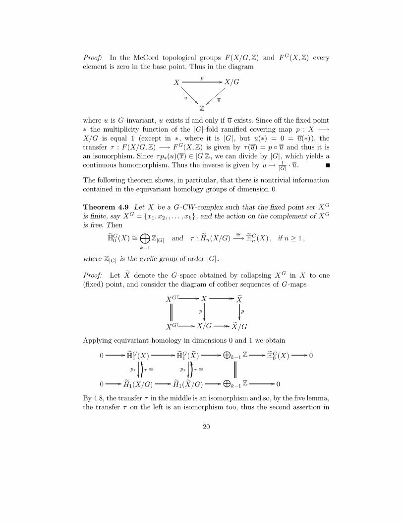
The following theorem shows, in particular, that there is nontrivial informationcontained in the equivariant homology groups of dimension 0.

Theorem 4.9 Let X be a G-CW-complex such that the fixed point set XG

is finite, say XG = {x1, x2, , . . . , xk}, and the action on the complement of XG

is free. Then

HG0 (X) ∼=

⊕

k−1

Z|G| and τ : Hn(X/G)∼=

−→ HGn (X) , if n ≥ 1 ,

where Z|G| is the cyclic group of order |G|.

Proof: Let X denote the G-space obtained by collapsing XG in X to one(fixed) point, and consider the diagram of cofiber sequences of G-maps

XG �

� // X // //

p

��

X

p

��

XG �

� // X/G // // X/G

Applying equivariant homology in dimensions 0 and 1 we obtain

0 // HG1 (X) //

p∗��

HG1 (X) //

p∗��

⊕k−1 Z // HG

0 (X) // 0

0 // H1(X/G) //

τ ∼=

TT

H1(X/G) //

τ ∼=

TT

⊕k−1 Z // 0

By 4.8, the transfer τ in the middle is an isomorphism and so, by the five lemma,the transfer τ on the left is an isomorphism too, thus the second assertion in

20

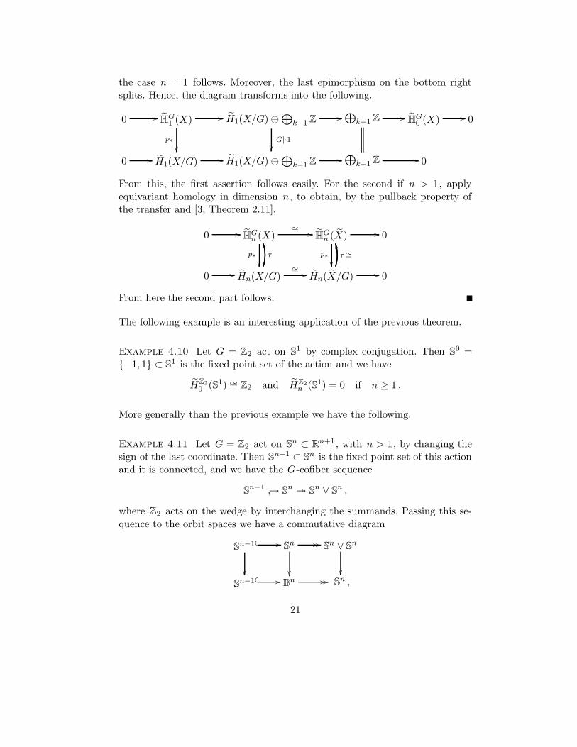
the case n = 1 follows. Moreover, the last epimorphism on the bottom rightsplits. Hence, the diagram transforms into the following.

0 // HG1 (X) //

p∗

��

H1(X/G) ⊕⊕

k−1 Z //

|G|·1��

⊕k−1 Z // HG

0 (X) // 0

0 // H1(X/G) // H1(X/G) ⊕⊕

k−1 Z //⊕

k−1 Z // 0

From this, the first assertion follows easily. For the second if n > 1, applyequivariant homology in dimension n, to obtain, by the pullback property ofthe transfer and [3, Theorem 2.11],

0 // HGn (X)

∼= //

p∗

��

HGn (X) //

p∗

��

0

0 // Hn(X/G)∼= //

τ

TT

Hn(X/G) //

τ ∼=

TT

0

From here the second part follows.

The following example is an interesting application of the previous theorem.

Example 4.10 Let G = Z2 act on S1 by complex conjugation. Then S0 ={−1, 1} ⊂ S1 is the fixed point set of the action and we have

HZ20 (S1) ∼= Z2 and HZ2

n (S1) = 0 if n ≥ 1 .

More generally than the previous example we have the following.

Example 4.11 Let G = Z2 act on Sn ⊂ Rn+1 , with n > 1, by changing thesign of the last coordinate. Then Sn−1 ⊂ Sn is the fixed point set of this actionand it is connected, and we have the G-cofiber sequence

Sn−1 ↪→ Sn � Sn ∨ Sn ,

where Z2 acts on the wedge by interchanging the summands. Passing this se-quence to the orbit spaces we have a commutative diagram

Sn−1 �

� //

��

Sn // //

��

Sn ∨ Sn

��Sn−1 �

� // Bn // // Sn ,

21

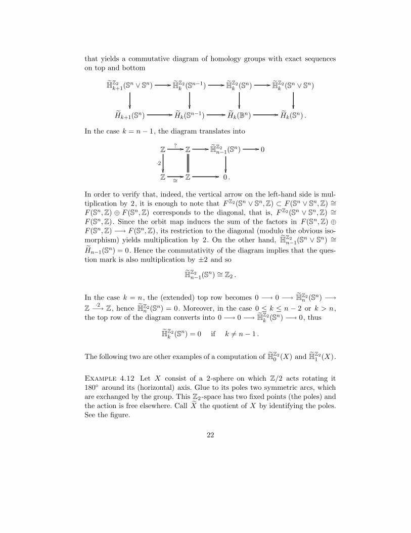
that yields a commutative diagram of homology groups with exact sequenceson top and bottom

HZ2k+1(S

n ∨ Sn) //

��

HZ2k (Sn−1) //

��

HZ2k (Sn) //

��

HZ2k (Sn ∨ Sn)

��

Hk+1(Sn) // Hk(S

n−1) // Hk(Bn) // Hk(S

n) .

In the case k = n− 1, the diagram translates into

Z? //

·2

��

Z // HZ2n−1(S

n) //

��

0

Z ∼=// Z // 0 .

In order to verify that, indeed, the vertical arrow on the left-hand side is mul-tiplication by 2, it is enough to note that F Z2(Sn ∨ Sn,Z) ⊂ F (Sn ∨ Sn,Z) ∼=F (Sn,Z) ⊕ F (Sn,Z) corresponds to the diagonal, that is, F Z2(Sn ∨ Sn,Z) ∼=F (Sn,Z). Since the orbit map induces the sum of the factors in F (Sn,Z) ⊕F (Sn,Z) −→ F (Sn,Z), its restriction to the diagonal (modulo the obvious iso-morphism) yields multiplication by 2. On the other hand, HZ2

n−1(Sn ∨ Sn) ∼=

Hn−1(Sn) = 0. Hence the commutativity of the diagram implies that the ques-

tion mark is also multiplication by ±2 and so

HZ2n−1(S

n) ∼= Z2 .

In the case k = n, the (extended) top row becomes 0 −→ 0 −→ HZ2n (Sn) −→

Z·2

−→ Z, hence HZ2n (Sn) = 0. Moreover, in the case 0 ≤ k ≤ n − 2 or k > n,

the top row of the diagram converts into 0 −→ 0 −→ HZ2k (Sn) −→ 0, thus

HZ2k (Sn) = 0 if k 6= n− 1 .

The following two are other examples of a computation of HZ20 (X) and HZ2

1 (X).

Example 4.12 Let X consist of a 2-sphere on which Z/2 acts rotating it180◦ around its (horizontal) axis. Glue to its poles two symmetric arcs, whichare exchanged by the group. This Z2 -space has two fixed points (the poles) andthe action is free elsewhere. Call X the quotient of X by identifying the poles.See the figure.

22

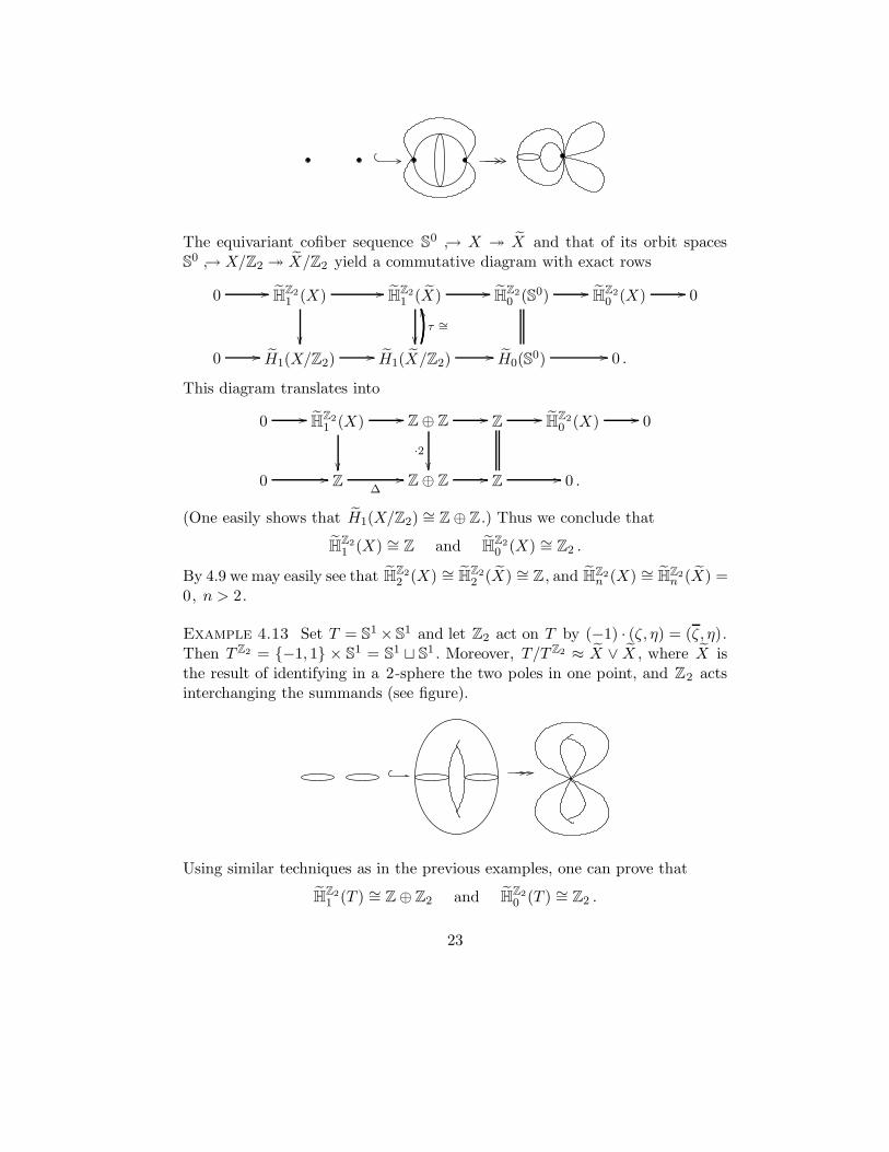
The equivariant cofiber sequence S0 ↪→ X � X and that of its orbit spacesS0 ↪→ X/Z2 � X/Z2 yield a commutative diagram with exact rows

0 // HZ21 (X) //

��

HZ21 (X) //

��

HZ20 (S0) // HZ2

0 (X) // 0

0 // H1(X/Z2)// H1(X/Z2)

//

τ ∼=

TT

H0(S0) // 0 .

This diagram translates into

0 // HZ21 (X) //

��

Z ⊕ Z //

·2

��

Z // HZ20 (X) // 0

0 // Z∆

// Z ⊕ Z // Z // 0 .

(One easily shows that H1(X/Z2) ∼= Z ⊕ Z.) Thus we conclude that

HZ21 (X) ∼= Z and HZ2

0 (X) ∼= Z2 .

By 4.9 we may easily see that HZ22 (X) ∼= HZ2

2 (X) ∼= Z, and HZ2n (X) ∼= HZ2

n (X) =0, n > 2.

Example 4.13 Set T = S1 × S1 and let Z2 act on T by (−1) · (ζ, η) = (ζ, η).Then T Z2 = {−1, 1} × S1 = S1 t S1 . Moreover, T/T Z2 ≈ X ∨ X , where X isthe result of identifying in a 2-sphere the two poles in one point, and Z2 actsinterchanging the summands (see figure).

Using similar techniques as in the previous examples, one can prove that

HZ21 (T ) ∼= Z ⊕ Z2 and HZ2

0 (T ) ∼= Z2 .

23

Once more these groups differ from the corresponding nonequivariant groups ofthe orbit spaces.

References

[1] M. Aguilar, S. Gitler, C. Prieto, Algebraic Topology from a Homotopical

Viewpoint, Universitexts, Springer-Verlag, New York Berlin Heidelberg, 2002.

[2] M. Aguilar, C. Prieto, Transfers for ramified coverings in homology andcohomology, International J. Math. And Math. Sci., 2006, Article ID 94651,(2006), 1–28.

[3] M. Aguilar, C. Prieto, A classification of cohomology transfers for ramifiedcovering maps, Fundamenta Math. 189 (2006), 1-25.

[4] E. Bredon, Equivariant Cohomology Theories, Lecture Notes in Math., No.34, Springer-Verlag, Heidelberg Berlin New York, 1967.

[5] E. Bredon, Introduction to Compact Transformation Groups, Academic Press,New York, London, 1972.

[6] K. Brown Cohomology of Groups, Graduate Texts in Mathematics, Springer-Verlag, New York Heidelberg Berlin, 1982.

[7] A. Dold, R. Thom Quasifaserungen und unendliche symmetrische Produkte,Annals of Math. 67 (1958), 239–281.

[8] S. Eilenberg, N. Steenrod, Foundations of Algebraic Topology, PrincetonUniv. Press, 1952.

[9] E. M. Friedlander, H. B. Lawson, Moving algebraic cycles of boundeddegree, Invent. Math. 132 (1998), 91–119.

[10] E. M. Friedlander, H. B. Lawson, Duality relating spaces of algebraiccocycles and cycles, Topology 36 (1997), 533–565.

[11] E. M. Friedlander, B. Mazur, Filtrations on the homology of algebraicvarieties. With an appendix by Daniel Quillen, Mem. Amer. Math. Soc. 110

(1994) no. 529, x+110 pages.

[12] J. P. C. Greenlees, J. P. May, Some remarks on the structure of Mackeyfunctors, Proc. Amer. Math. Soc. 115 (1992), 237–243.

[13] S. Illman, Equivariant singular homology and cohomology I, Memoirs of the

Amer. Math. Soc. Vol. 1, Issue 2, No. 156, 1975.

[14] H. B. Lawson, Jr., Algebraic cycles and homotopy theory, Annals of Math.

129 (1989), 253–291.

[15] H. B. Lawson, Jr., Spaces of algebraic cycles: levels of holomorphic approxi-mation. Proceedings of the International Congress of Mathematicians, Vol. 1, 2(Zurich, 1994), 574–584, Birkhauser, Basel, 1995.

24

[16] P. Lima-Filho, On the equivariant homotopy of free abelian on G-spaces andG-spectra, Math. Z. 224 (1997), 567-601.

[17] J. P. May, Simplicial Objects in Algebraic Topology, The University of ChicagoPress, Chicago London, 1992

[18] J. P. May, A Concise Course in Algebraic Topology, The University of ChicagoPress, Chicago London, 1999.

[19] M. C. McCord, Classifying spaces and infinite symmetric products, Trans.

Amer. Math. Soc. 146 (1969), 273–298.

[20] F. Rhodes, On the fundamental group of a transformation group, Proc. London

Math. Soc. 16 (1966), 635–650.

[21] P. F. dos Santos, A note on the equivariant Dold-Thom theorem, J. Pure

Appl. Algebra 183 (2003), 299–312.

[22] S. J. Willson, Equivariant homology theories on G-complexes, Trans. Amer.

Math. Soc. 212 (1975), 155–171

October 5, 2006

25