Due Wednesday, 4/12/17 - Union Collegeminerva.union.edu/labrakes/Phy220_HW2S_Full_S17.pdf · Due...
13
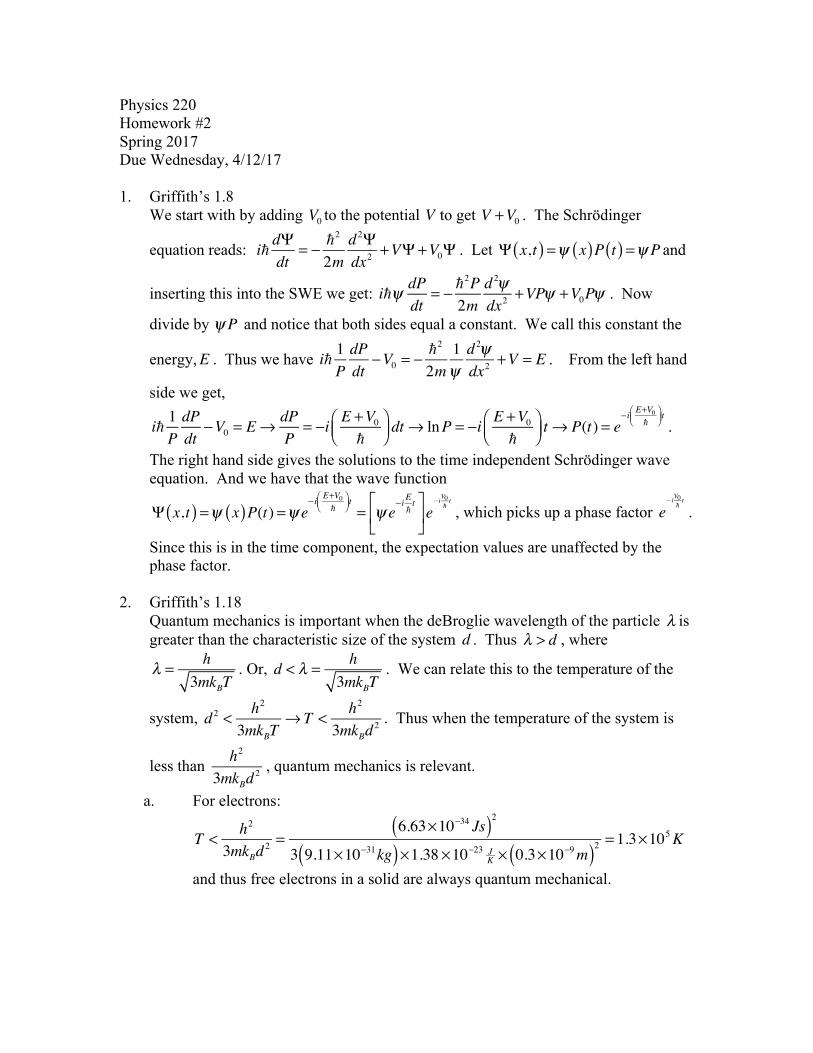
Physics 220 Homework #2 Spring 2017 Due Wednesday, 4/12/17 1. Griffith’s 1.8 We start with by adding V 0 to the potential V to get V + V 0 . The Schrödinger equation reads: i! dΨ dt = − ! 2 2 m d 2 Ψ dx 2 + V Ψ + V 0 Ψ . Let Ψ x, t ( ) = ψ x () Pt () = ψ P and inserting this into the SWE we get: i!ψ dP dt = − ! 2 P 2 m d 2 ψ dx 2 + VP ψ + V 0 P ψ . Now divide by ψ P and notice that both sides equal a constant. We call this constant the energy, E . Thus we have i! 1 P dP dt − V 0 = − ! 2 2 m 1 ψ d 2 ψ dx 2 + V = E . From the left hand side we get, i! 1 P dP dt − V 0 = E → dP P = −i E + V 0 ! ⎛ ⎝ ⎜ ⎞ ⎠ ⎟ dt → ln P = −i E + V 0 ! ⎛ ⎝ ⎜ ⎞ ⎠ ⎟ t → P(t ) = e − i E+V 0 ! ⎛ ⎝ ⎜ ⎞ ⎠ ⎟ t . The right hand side gives the solutions to the time independent Schrödinger wave equation. And we have that the wave function Ψ x, t ( ) = ψ x () P(t ) = ψ e − i E+V 0 ! ⎛ ⎝ ⎜ ⎞ ⎠ ⎟ t = ψ e − i E ! t ⎡ ⎣ ⎢ ⎤ ⎦ ⎥ e − i V 0 ! t , which picks up a phase factor e − i V 0 ! t . Since this is in the time component, the expectation values are unaffected by the phase factor. 2. Griffith’s 1.18 Quantum mechanics is important when the deBroglie wavelength of the particle λ is greater than the characteristic size of the system d . Thus λ > d , where λ = h 3mk B T . Or, d < λ = h 3mk B T . We can relate this to the temperature of the system, d 2 < h 2 3mk B T → T < h 2 3mk B d 2 . Thus when the temperature of the system is less than h 2 3mk B d 2 , quantum mechanics is relevant. a. For electrons: T < h 2 3mk B d 2 = 6.63 × 10 −34 Js ( ) 2 3 9.11 × 10 −31 kg ( ) × 1.38 × 10 −23 J K × 0.3 × 10 −9 m ( ) 2 = 1.3 × 10 5 K and thus free electrons in a solid are always quantum mechanical.
Transcript of Due Wednesday, 4/12/17 - Union Collegeminerva.union.edu/labrakes/Phy220_HW2S_Full_S17.pdf · Due...
Physics 220 Homework #2 Spring 2017 Due Wednesday, 4/12/17 1. Griffith’s 1.8
We start with by adding V0 to the potential V to get V +V0 . The Schrödinger
equation reads: i! dΨ
dt= − !
2
2md 2Ψdx2
+VΨ +V0Ψ . Let Ψ x,t( ) =ψ x( )P t( ) =ψ P and
inserting this into the SWE we get: i!ψ dP
dt= − !
2P2m
d 2ψdx2
+VPψ +V0Pψ . Now
divide by ψ P and notice that both sides equal a constant. We call this constant the
energy,E . Thus we have i! 1PdPdt
−V0 = − !2
2m1ψd 2ψdx2
+V = E . From the left hand
side we get,
i! 1PdPdt
−V0 = E→ dPP
= −i E +V0!
⎛⎝⎜
⎞⎠⎟ dt→ lnP = −i E +V0
!⎛⎝⎜
⎞⎠⎟ t→ P(t) = e
− i E+V0!
⎛⎝⎜
⎞⎠⎟ t .
The right hand side gives the solutions to the time independent Schrödinger wave equation. And we have that the wave function
Ψ x,t( ) =ψ x( )P(t) =ψ e
− i E+V0!
⎛⎝⎜
⎞⎠⎟ t = ψ e
− i E!t⎡
⎣⎢
⎤
⎦⎥e
− iV0!t
, which picks up a phase factor e− iV0!t
.
Since this is in the time component, the expectation values are unaffected by the phase factor.
2. Griffith’s 1.18 Quantum mechanics is important when the deBroglie wavelength of the particle λ is greater than the characteristic size of the system d . Thus λ > d , where
λ = h3mkBT
. Or, d < λ = h3mkBT
. We can relate this to the temperature of the
system, d 2 < h2
3mkBT→ T < h2
3mkBd2 . Thus when the temperature of the system is
less than h2
3mkBd2 , quantum mechanics is relevant.
a. For electrons:
T < h2
3mkBd2 =
6.63×10⁻³⁴ Js( )23 9.11×10⁻³¹kg( )×1.38 ×10⁻²³ J
K × 0.3×10⁻⁹m( )2= 1.3×10⁵K
and thus free electrons in a solid are always quantum mechanical.
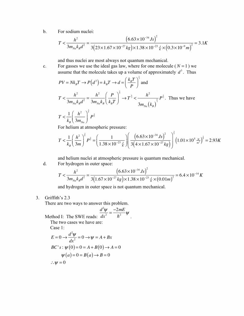
b. For sodium nuclei:
T < h2
3mNakBd2 =
6.63×10⁻³⁴ Js( )23 23×1.67 ×10−27 kg( )×1.38 ×10⁻²³ J
K × 0.3×10⁻⁹m( )2= 3.1K
and thus nuclei are most always not quantum mechanical.
c. For gasses we use the ideal gas law, where for one molecule (N = 1 ) we assume that the molecule takes up a volume of approximately d 3 . Thus
PV = NkBT → P d 3( ) = kBT → d = kBTP
⎛⎝⎜
⎞⎠⎟
13
and
T < h2
3mNakBd2 =
h2
3mNakBPkBT
⎛⎝⎜
⎞⎠⎟
23
→ T53 < h2
3mNa kB( )53P
23 . Thus we have
T < 1kB
h2
3mNa
⎛⎝⎜
⎞⎠⎟
35
P25
For helium at atmospheric pressure:
T < 1kB
h2
3m⎛⎝⎜
⎞⎠⎟
35
P25 = 1
1.38 ×10⁻²³ JK
⎛⎝⎜
⎞⎠⎟
6.63×10⁻³⁴ Js( )23 4 ×1.67 ×10−27 kg( )
⎛
⎝⎜⎜
⎞
⎠⎟⎟
35
1.01×10⁵ Nm2( )25 = 2.93K
and helium nuclei at atmospheric pressure is quantum mechanical.
d. For hydrogen in outer space:
T < h2
3mNakBd2 =
6.63×10⁻³⁴ Js( )23 1.67 ×10⁻²⁷ kg( )×1.38 ×10⁻²³ J
K × 0.01m( )2= 6.4 ×10⁻¹⁴K
and hydrogen in outer space is not quantum mechanical.
3. Griffith’s 2.3 There are two ways to answer this problem.
Method I: The SWE reads:
d 2ψdx2
= −2mE!2
ψ.
The two cases we have are: Case 1:
E = 0→ d 2ψdx2
= 0→ψ = A + Bx
BC 's :ψ 0( ) = 0 = A + B 0( )→ A = 0ψ a( ) = 0 = B a( )→ B = 0
∴ψ = 0
Case 2:
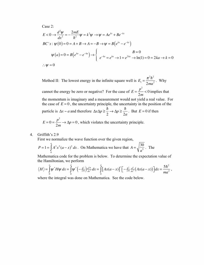
Method II: The lowest energy in the infinite square well is E1 =
π 2!2
2ma2. Why
cannot the energy be zero or negative? For the case of E = p2
2m< 0 implies that
the momentum is imaginary and a measurement would not yield a real value. For the case of E = 0 , the uncertainty principle, the uncertainty in the position of the
particle is Δx ~ a and therefore ΔxΔp ≥ !
2→Δp ≥ !
2a. But E = 0 if then
E = 0 = p2
2m→Δp = 0 , which violates the uncertainty principle.
4. Griffith’s 2.9
First we normalize the wave function over the given region,
P = 1= A2x2 (a − x)2 dx0
a
∫ . On Mathematica we have that A = 30a5
. The
Mathematica code for the problem is below. To determine the expectation value of the Hamiltonian, we perform
H = ψ *Hψ dx
0
a
∫ = ψ * − !22m( ) d2ψdx2 dx
0
a
∫ = Ax(a − x)[ ]* − !22m
d2
dx2 Ax(a − x)( )⎡⎣ ⎤⎦dx0
a
∫ = 5!2
ma2,
where the integral was done on Mathematica. See the code below.
E < 0→ d 2ψdx2
= − 2mE!2
ψ = k2ψ →ψ = Aekx + Be−kx
BC 's :ψ 0( ) = 0 = A + B→ A = −B→ψ = B ekx − e−kx( )
ψ a( ) = 0 = B eka − e−ka( )→ B = 0e−ka = eka →1= e2ka → ln(1) = 0 = 2ka→ k = 0
⎧⎨⎪
⎩⎪∴ψ = 0
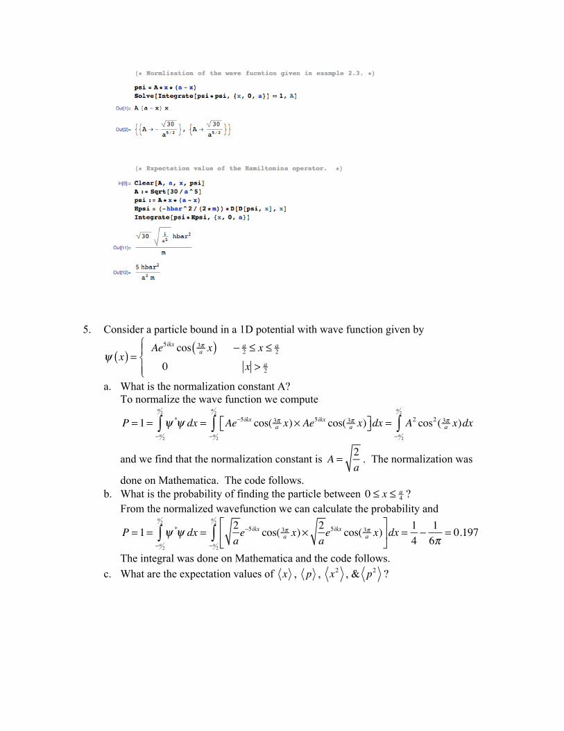
5. Consider a particle bound in a 1D potential with wave function given by
ψ x( ) =Ae5ikx cos 3π
a x( ) − a2 ≤ x ≤ a
2
0 x > a2
⎧⎨⎪
⎩⎪
a. What is the normalization constant A? To normalize the wave function we compute
P = 1= ψ *ψ dx−a 2
a2
∫ = Ae−5ikx cos( 3πa x)× Ae5ikx cos( 3πa x)⎡⎣ ⎤⎦dx
−a 2
a2
∫ = A2 cos2( 3πa x)dx−a 2
a2
∫
and we find that the normalization constant is A = 2a
. The normalization was
done on Mathematica. The code follows. b. What is the probability of finding the particle between 0 ≤ x ≤ a
4 ? From the normalized wavefunction we can calculate the probability and
P = 1= ψ *ψ dx−a 2
a2
∫ = 2ae−5ikx cos( 3πa x)×
2ae5ikx cos( 3πa x)
⎡
⎣⎢
⎤
⎦⎥dx
−a 2
a2
∫ = 14− 16π
= 0.197
The integral was done on Mathematica and the code follows. c. What are the expectation values of x , p , x2 , & p2 ?
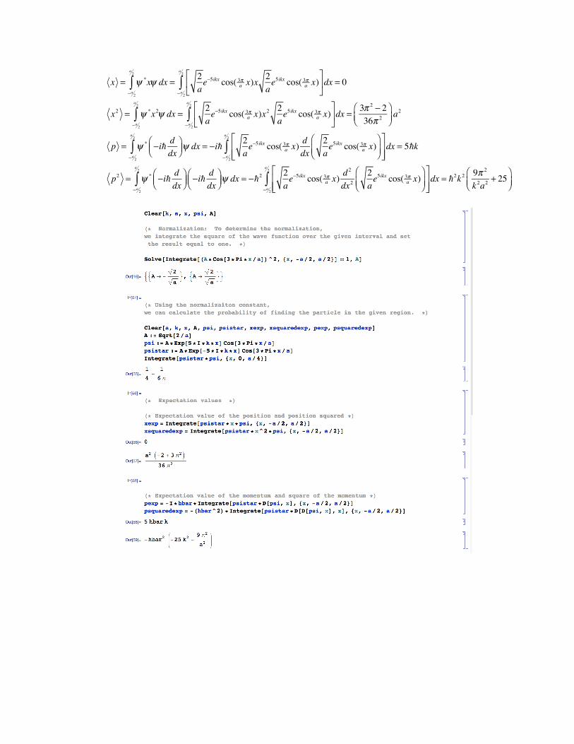
x = ψ *xψ dx−a 2
a2
∫ = 2ae−5ikx cos( 3πa x)x
2ae5ikx cos( 3πa x)
⎡
⎣⎢
⎤
⎦⎥dx
−a 2
a2
∫ = 0
x2 = ψ *x2ψ dx−a 2
a2
∫ = 2ae−5ikx cos( 3πa x)x
2 2ae5ikx cos( 3πa x)
⎡
⎣⎢
⎤
⎦⎥dx
−a 2
a2
∫ = 3π 2 − 236π 2
⎛⎝⎜
⎞⎠⎟a2
p = ψ * −i! ddx
⎛⎝⎜
⎞⎠⎟ψ dx
−a 2
a2
∫ = −i! 2ae−5ikx cos( 3πa x)
ddx
2ae5ikx cos( 3πa x)
⎛⎝⎜
⎞⎠⎟
⎡
⎣⎢⎢
⎤
⎦⎥⎥dx
−a 2
a2
∫ = 5!k
p2 = ψ * −i! ddx
⎛⎝⎜
⎞⎠⎟ −i! d
dx⎛⎝⎜
⎞⎠⎟ψ dx
−a 2
a2
∫ = −!2 2ae−5ikx cos( 3πa x)
d 2
dx22ae5ikx cos( 3πa x)
⎛⎝⎜
⎞⎠⎟
⎡
⎣⎢⎢
⎤
⎦⎥⎥dx
−a 2
a2
∫ = !2k2 9π 2
k2a2+ 25
⎛⎝⎜
⎞⎠⎟
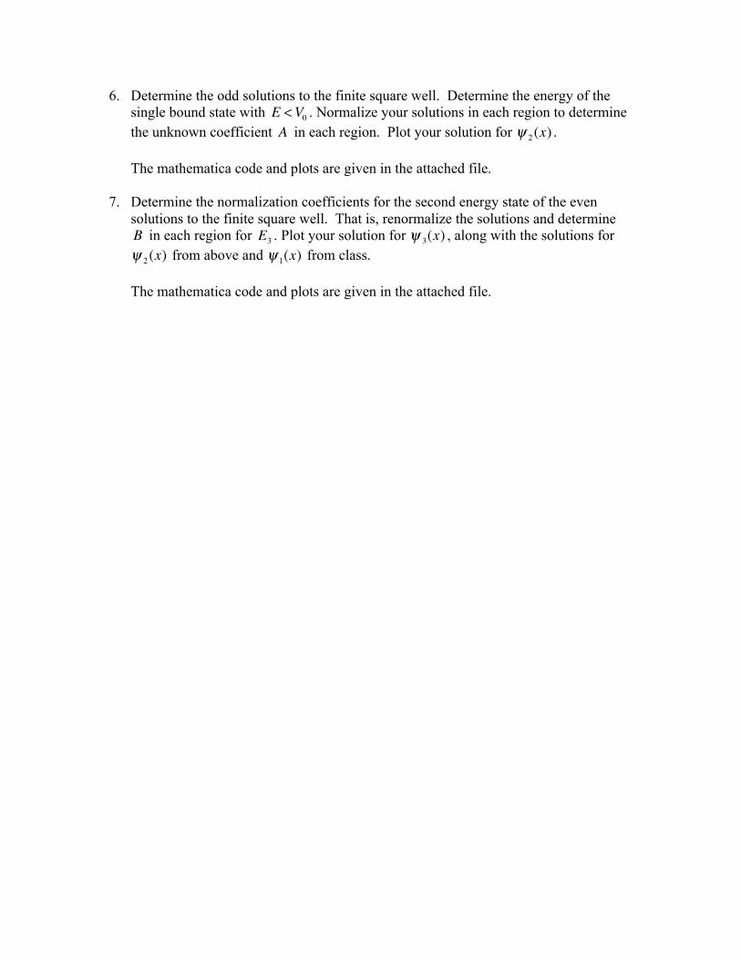
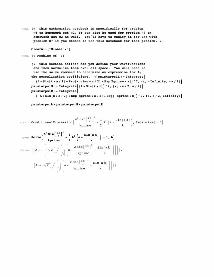
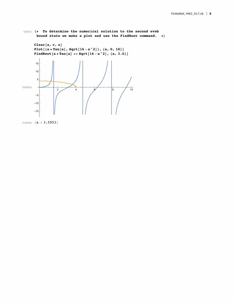
6. Determine the odd solutions to the finite square well. Determine the energy of the single bound state with E <V0 . Normalize your solutions in each region to determine the unknown coefficient A in each region. Plot your solution for ψ 2 (x) . The mathematica code and plots are given in the attached file.
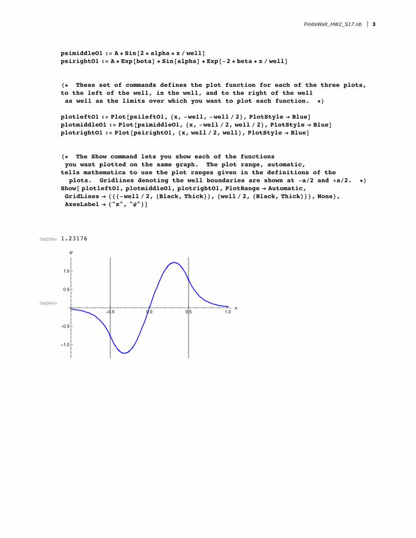
7. Determine the normalization coefficients for the second energy state of the even solutions to the finite square well. That is, renormalize the solutions and determine B in each region for E3 . Plot your solution for ψ 3(x) , along with the solutions for ψ 2 (x) from above and ψ 1(x) from class. The mathematica code and plots are given in the attached file.
��������� (* ���� ����������� �������� �� ������������ ��� �������
#� �� �������� ��� #�� �� ��� ���� �� ���� ��� ������� #� ��
�������� ��� #� �� ����� ������ ���� �� ������ �� ��� ��� ����
������� #� �� ��� ������ �� ��� ���� �������� ��� ���� �������� *)
��������[��������*�]
��������� (* ������� #� *)
(* ���� ������� ������� ��� ��� ������ ���� �������������
��� ���� ��������� ���� ���� ��� ������ ��� ���� ���� ��
��� ��� ����� ������� �� ��������� �� ���������� ��� ��
��� ������������� ������������ *)����������� �= ���������
� * ���[� * � / �] * ���[������ * � / �] * ���[������ * �]��� {�� -��������� -� / �}
����������� �= ���������� * ���[� * �]��� {�� -� / �� � / �}
����������� �= ���������
-� * ���[� * � / �] * ���[������ * � / �] * ���[-������ * �]��� {�� � / �� ��������}
����������� + ����������� + �����������
��������� ����������������������� ��� � �
��
������+�
��� � -
���[� �]
�� ��[������] > �
��������� ������� ��� � �
��
������+�
��� � -
���[� �]
�⩵ �� �
��������� � → - � � +� ��� � �
��
������-���[� �]
��
� → � � +� ��� � �
��
������-���[� �]
�

��������� (* �� ��������� ��� ��������� �������� �� ��� ���
����� ����� �� ���� � ���� ��� ��� ��� �������� �������� *)
�����[�� �� �]
����[{-� * ���[�]� ����[�� - ���]}� {�� �� ��}]
��������[-� * ���[�] == ����[�� - ���]� {�� ���}]
���������
2 4 6 8 10
-15
-10
-5
5
10
15
��������� {� → �������}
(* ������ ��� ���� ��� ��� ��������� ��� � ������ ���� ���� � = �� *)
�����[�� ������ �� ����� ����� ���������� ������������
����������� ����������� ������������� �����������]
(* ������ ��� ������������� ������������ ��� ���� �� ����� ����
���������� ��� ��� ������������� ����������� ��� ����� �� ������ *)
� �= ����[� / ����] * ���[�����]�� ���� + � - ���[� * �����] (� * �����)�(-� / �)
(* ������ ������ �����
� ��� ��� ����� �� ��� ����� ���� ��� ���� ��� ������ �� -�/� �� �/��
����� ��� ����� ����� ��� ���� �� ��� �������� ����� �����������
�� �������� ��� ���������� ��� �� ��� ������� ��� ������� ���
������������� ����������� ���� �� ��������� ������� ��� ����
�� ��������� ����� ��� ��� ��� �������� ��� ����� �� ����� *)
(* ��� �� ��� ��� ����� �� � ��� ����������� ����� ��� ������ �� �� ������*)
����� �= ������
� �= �
���� �= ����[��� - �������]
���� �= �
�
(* ���� ������� ��� ������������ �� ���� �� ��� �����
�������� ������� �� ��� ����������� �� ��� ���� �� ��� �����
��������� �� ��� ������������ �� ��� �����
��� �������� �� ��� ������������ �� ��� ����� �� ��� ����� ��� ����
�� ����� ���� ����������� ��� ��� ������������� �� ���� �������*)
��������� �= -� * ���[����] * ���[�����] * ���[� * ���� * � / ����]
2 ��� FiniteWell_HW2_S17.nb
����������� �= � * ���[� * ����� * � / ����]
���������� �= � * ���[����] * ���[�����] * ���[-� * ���� * � / ����]
(* ����� ��� �� �������� ������� ��� ���� �������� ��� ���� �� ��� ����� ������
�� ��� ���� �� ��� ����� �� ��� ����� ��� �� ��� ����� �� ��� ����
�� ���� �� ��� ������ ���� ����� ��� ���� �� ���� ���� ��������� *)
���������� �= ����[���������� {�� -����� -���� / �}� ��������� → ����]
������������ �= ����[������������ {�� -���� / �� ���� / �}� ��������� → ����]
����������� �= ����[����������� {�� ���� / �� ����}� ��������� → ����]
(* ��� ���� ������� ���� ��� ���� ���� �� ��� ���������
��� ���� ������� �� ��� ���� ������ ��� ���� ������ ����������
����� ����������� �� ��� ��� ���� ������ ����� �� ��� ����������� �� ���
������ ��������� �������� ��� ���� ���������� ��� ����� �� -�/� ��� +�/�� *)
����[ ����������� ������������� ������������ ��������� → ����������
��������� → {{{-���� / �� {������ �����}}� {���� / �� {������ �����}}}� ����}�
��������� → {���� �ψ�}]
��������� �������
���������
-0.5 0.0 0.5 1.0x
-1.0
-0.5
0.5
1.0
ψ
FiniteWell_HW2_S17.nb ���3
���������
(* ������� #� *)
(* ���� ����� ��� ������������� ��������� ��� ��� ����
���������� ���� �� ��� ���� ���� ���� � ���� �� ����� *)
�����[�� �� �� �� �����]
����������� �= ���������
� * ���[� * � / �] * ���[������ * � / �] * ���[������ * �]��� {�� -��������� -� / �}
����������� �= ���������[(� * ���[� * �])��� {�� -� / �� � / �}]
����������� �= ���������
� * ���[� * � / �] * ���[������ * � / �] * ���[-������ * �]��� {�� � / �� ��������}
����������� + ����������� + �����������
��������� ����������������������� ��� � �
��
������+�� � � + ���[� �]
� �� ��[������] > �
��������� ������� ��� � �
��
������+�� � � + ���[� �]
� �⩵ �� �
��������� � → - � � +� ��� � �
��
������+���[� �]
��
� → � � +� ��� � �
��
������+���[� �]
�
(* ��� ��� ������ ���� ��������� �� ��� ������ ����� *)
4 ��� FiniteWell_HW2_S17.nb
��������� (* �� ��������� ��� ��������� �������� �� ��� ������ ����
����� ����� �� ���� � ���� ��� ��� ��� �������� �������� *)
�����[�� �� �]
����[{� * ���[�]� ����[�� - ���]}� {�� �� ��}]
��������[� * ���[�] == ����[�� - ���]� {�� ���}]
���������2 4 6 8 10
-15
-10
-5
5
10
15
��������� {� → ������}
FiniteWell_HW2_S17.nb ���5

��������� (* ������ ��� ���� ��� ������ ���� �������� ��� � ������ ���� ���� � = �� *)
�����[�� ������ �� ����� ����� ���������� ������������
����������� ����������� ������������� �����������]
(* ������ ��� ������������� ����������� ���� ��� ���������� ����� *)
� �= ����[� / ����] * ���[�����]�� ���� + � - ���[� * �����] (� * �����)�(-� / �)
(* ������ ������ �����
� ��� ��� ����� �� ��� ����� ���� ��� ���� ��� ������ �� -�/� �� �/�� *)
(* ��� �� ��� ��� ����� �� � ��� ����������� ����� ��� ������ �� �� ������*)
����� �= ������
� �= �
���� �= ����[��� - �������]
���� �= �
�
(* ���� ������� ��� ������������ �� ���� �� ��� �����
�������� ������� �� ��� ����������� �� ��� ���� �� ��� �����
��������� �� ��� ������������ �� ��� �����
��� �������� �� ��� ������������ �� ��� ����� �� ��� ����� ��� ����
�� ����� ���� ����������� ��� ��� ������������� �� ���� �������*)
��������� �= � * ���[����] * ���[�����] * ���[� * ���� * � / ����]
����������� �= � * ���[� * ����� * � / ����]
���������� �= � * ���[����] * ���[�����] * ���[-� * ���� * � / ����]
(* ����� ��� �� �������� ������� ��� ���� �������� ��� ���� �� ��� ����� ������
�� ��� ���� �� ��� ����� �� ��� ����� ��� �� ��� ����� �� ��� ����
�� ���� �� ��� ������ ���� ����� ��� ���� �� ���� ���� ��������� *)
���������� �= ����[���������� {�� -����� -���� / �}� ��������� → �����]
������������ �= ����[������������ {�� -���� / �� ���� / �}� ��������� → �����]
����������� �= ����[����������� {�� ���� / �� ����}� ��������� → �����]
��������� �������
6 ��� FiniteWell_HW2_S17.nb
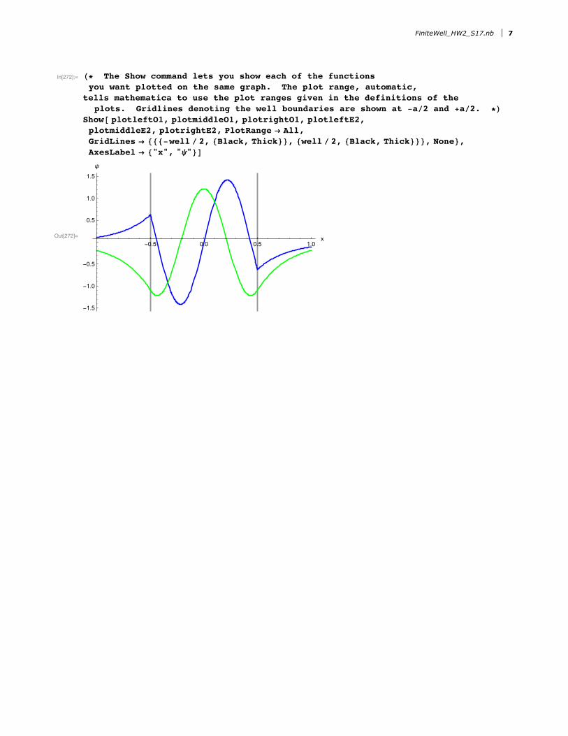
��������� (* ��� ���� ������� ���� ��� ���� ���� �� ��� ���������
��� ���� ������� �� ��� ���� ������ ��� ���� ������ ����������
����� ����������� �� ��� ��� ���� ������ ����� �� ��� ����������� �� ���
������ ��������� �������� ��� ���� ���������� ��� ����� �� -�/� ��� +�/�� *)
����[ ����������� ������������� ������������ �����������
������������� ������������ ��������� → ����
��������� → {{{-���� / �� {������ �����}}� {���� / �� {������ �����}}}� ����}�
��������� → {���� �ψ�}]
���������
-0.5 0.0 0.5 1.0x
-1.5
-1.0
-0.5
0.5
1.0
1.5
ψ
FiniteWell_HW2_S17.nb ���7