Discrete-Time Martingalesocw.nctu.edu.tw/upload/classbfs120912252641448.pdf · CHAPTER 2...

CHAPTER 2

Discrete-Time Martingales

2.1. Conditional probability and conditional expectation

2.1.1. Conditional expectation with respect to a set. Let (Ω,F , P) be a prob-

ability space.

Recall: If the sets A,B ∈ F and P(B) > 0, the conditional probability of A with

respect to B is defined by

P(A|B) =P(A ∩ B)

P(B).

Remark 2.1. The set function P(·|B) : F −→ R is a probability measure.

Definition 2.2. The conditional expectation of a random variable X given B is defined

as the expectation of X with respect to the conditional probability P(·|B).

Example 2.3. Consider a probability space with

Ω = {1, 2, 3, 4} F = σ({1}, {2}, {3}, {4}),

and the probability measure

P({1}) =1

2, P({2}) =

1

4, P({3}) =

1

6, P({4}) =

1

12.

Let B = {1, 2, 3}, then

P(A|B) =P(A ∩ B)

P(B)=

P(A ∩ B)1

2+

1

4+

1

6

=12

11P(A ∩ B).

23

24 2. DISCRETE-TIME MARTINGALES

This implies that

P({1}|B) =12

11P({1}) =

6

11,

P({2}|B) =12

11P({2}) =

3

11,

P({3}|B) =12

11P({3}) =

2

11,

P({4}|B) =12

11P({4}) = 0.

Let X(1) = 4, X(2) = 3, X(3) = 2, X(4) = 1. Then

E[X] = X(1) · P({1}) + X(2) · P({2}) + X(3) · P({3}) + X(4) · P({4})

= 4 · 1

2+ 3 · 1

4+ 2 · 1

6+ 1 · 1

12=

19

6,

E[X|B] = X(1) · P({1}|B) + X(2) · P({2}|B) + X(3) · P({3}|B) + X(4) · P({4}|B)

= 4 · 6

11+ 3 · 3

11+ 2 · 2

11+ 1 · 0 =

37

11.

��: �� E[X] �� X ��

� / ��; �� E[X|B] �� X �� B ��, �

�, ��; ��.

2.1.2. Conditional expectation with respect to random variable.

Definition 2.4. Let X and Y be discrete random variables on (Ω,F , P) and assume

that P(Y = y) > 0. Suppose that p(x, y) is the joint mass function of X and Y and pY is

the probability mass function of Y ; explicitly,

pY (y) =∑

x

p(x, y).

2.1. CONDITIONAL PROBABILITY AND CONDITIONAL EXPECTATION 25

(1) The function

pX|Y (x|y) = P(X = x|Y = y) = P({ω : X(ω) = x}|{ω : Y (ω) = y})

=P(X = x, Y = y)

P(Y = y)=

p(x, y)

pY (y)

is called the conditional probability mass function of X given that Y = y.

(2) The conditional expectation of X, given that Y = y (for all values of y such that

P(Y = y) > 0), is defined by

E[X|Y = y] =∑

x

P(X = x|Y = y) =∑

x

xP(X = x, Y = y)

P(Y = y)

=∑

x

xp(x, y)

pY (y).

Example 2.5. (1) Consider Ω = {1, 2, 3} and F is the collection of all subsets of

Ω. Moreover,

P({1}) =1

2, P({2}) =

1

3, P({3}) =

1

6.

Suppose X(ω) = ω, Y (ω) = 4 − ω. Then

p(1, 1) = p(1, 2) = 0, p(1, 3) =1

2,

p(2, 1) = p(2, 3) = 0, p(2, 2) =1

3,

p(3, 2) = p(3, 3) = 0, p(3, 1) =1

6,

and

pY (1) =1

6, pY (2) =

1

3, pY (3) =

1

2.


Thus,

pX|Y (1|1) = pX|Y (1|2) = 0, pX|Y (1|3) = 1,

pX|Y (2|1) = pX|Y (2|3) = 0, pX|Y (2|2) = 1,

pX|Y (3|2) = pX|Y (3|3) = 0, pX|Y (3|1) = 1.

(2) Suppose that the joint probability mass function of X and Y is given by

p(1, 1) =1

12, p(1, 2) =

1

24, p(1, 3) =

1

48,

p(1, 1) =1

6, p(2, 2) =

1

8, p(2, 3) =

1

16,

p(3, 1) =1

4, p(3, 2) =

1

12, p(3, 3) =

1

6.

Then

pY (1) = p(1, 1) + p(2, 1) + p(3, 1) =1

12+

1

6+

1

4=

1

2,

pY (2) = p(1, 2) + p(2, 2) + p(3, 2) =1

24+

1

8+

1

12=

1

4,

pY (3) = p(1, 3) + p(2, 3) + p(3, 3) =1

48+

1

16+

1

6=

1

4.

Thus,

pX|Y (1|1) =1

6, pX|Y (1|2) =

1

6, pX|Y (1|3) =

1

12,

pX|Y (2|1) =1

3, pX|Y (2|2) =

1

2, pX|Y (2|3) =

1

4,

pX|Y (3|1) =1

2, pX|Y (3|2) =

1

3, pX|Y (3|3) =

2

3.


This implies that

E[X|Y = 1] = 1 · pX|Y (1|1) + 2 · pX|Y (2|1) + 3 · pX|Y (3|1) =7

3,

E[X|Y = 2] = 1 · pX|Y (1|2) + 2 · pX|Y (2|2) + 3 · pX|Y (3|2) =13

6,

E[X|Y = 3] = 1 · pX|Y (1|3) + 2 · pX|Y (2|3) + 3 · pX|Y (3|3) =31

6.

��: �� random variables ��? ��

�� Y � distribution ��, P(Y = y) = 0, ��. ��

��. �� P(X = x|Y = y), ��

P(x ≤ X < x +�x|y ≤ Y < y +�y), �� y → 0. Let X and Y be jointly continuous

random variables with joint probability density function f(x, y). ��

P(x ≤ X < x + �x|y ≤ Y < y + �y) =P(x ≤ X < x + �x, y ≤ Y < y + �y)

P(y ≤ Y < y + �y)

=

∫ x+�x

x

∫ y+�y

y

f(x, y) dy dx∫ y+�y

y

fY (y) dy

−→

∫ x+�x

x

f(x, y) dx

fY (y),

as �y → ∞. Thus, we can have the following definition.

Definition 2.6. (1) The conditional probability density function of X, given that

Y = y, is defined for all valued of y such that fY (y) > 0 by

fX|Y (x|y) =f(x, y)

fY (y).

(2) The conditional expectation of X, given that Y = y, is defined by

E[X|Y = y] =

∫ ∞

−∞xfX|Y (x|y) dx,


provided that fY (y) > 0.

Remark 2.7. Let g be a Borel measurable function. Then

E[g(X)|Y = y] =

∫ ∞

−∞g(x)fX|Y (x|y) dx.

Example 2.8. Suppose that the joint density function of X and Y is given by

f(x, y) =1

yexp

(−x

y− y

)0 < x, y < ∞.

Compute E[X|Y = y] and E[X2|Y = y].

Solution. The marginal density function of Y is given by

fY (y) =

∫ ∞

0

f(x, y) dx =

∫ ∞

0

1

yexp

(−x

y− y

)dx

= e−y(−e−x/y

)∣∣∞x=0

= e−y.

Thus,

fX|Y (x|y) =f(x, y)

fY (y)=

1

ye−

xy .

Then

E[X|Y = y] =

∫ ∞

−∞xfX|Y (x|y) dx =

∫ ∞

0

x

ye−

xy dx = · · · = y

E[X2|Y = y] =

∫ ∞

−∞x2fX|Y (x|y) dx =

∫ ∞

0

x2

ye−

xy dx = · · · = 2y2.

Notation 2.9. Denote E[X|Y ] by the function of the random variable Y whose value

at Y = y is E[X|Y = y].

Example 2.10. As in Example 2.8,

E[X|Y ] = Y, E[X2|Y ] = 2Y 2.

Remark 2.11. E[X|Y ] is a random variable.


E[X|Y ]�� conditional expectation�� . ��

sample space Ω� decomposition�� decomposition��. decomposition

� conditional expectation ��. �� σ-algebra ��

��.

��, � E[X|A]. ��

��, ��?

2.1.3. Conditional expectation with respect to decomposition.

� E[X|Y ] E[X|Y = y] ��? �� Y discrete random

variable � case. �� E[X|Y = y] ��, E[X|Y ] �� y � Y ��.

�� Y � discrete random variable (i.e., Y �� countable ��) ��

� E[X|Y ](ω) � E[X|Y (ω)], � E[X|Y = y] (for Y (ω) = y). ��

E[X|Y ] = E[X|Y = y1] I{Y =y1} + E[X|Y = y2]I{Y =y2} + · · ·

=∞∑i=1

E[X|Y = yi] I{Y =yi}

��? � {Y = yi} �, E[X|Y ] �� E[X|Y = yi], X � {Y = yi} ��. ��

�, ��.

2.1.3.1. Conditional probability with respect to the decomposition of a

sample space. Consider a probability space (Ω,F , P). Let D = {D1, D2, ..., Dn} satisfy

(1) D is a decomposition of Ω, i.e.,

D1 ∪ D2 ∪ · · · ∪ Dn = Ω, Di ∩ Dj = ∅ for i = j;

(2) Di ∈ F for all i;


(3) P(Di) > 0 for all i.

Therefore, for A ∈ F , the conditional probability P(A|Di) is well-defined for all i.

Definition 2.12. The conditional probability of a set A ∈ F with respect to the

decomposition D is defined by

P(A|D) =n∑

i=1

P(A|Di) IDi.

Example 2.13. Consider ([0, 1],B1,m), A = [1/2, 3/4] and

D = {[0, 1.3], (1/3, 2/3), [2/3, 1]}.

Then

P(a|D) = P(A|[0, 1/3]) I[0,1/3] + P(A|(1/3, 2/3)) I(1/3,2/3) + P(A|[2/3, 1]) I[2/3,1]

=P([1/2, 2/3))

P((1/3, 2/3))I(1/3,2/3) +

P([2/3, 3/4])

P([2/3, 1])I[2/3,1]

=1

2I(1/3,2/3) +

1

4I[2/3,1].

Remark 2.14. (1) If D = {Ω}, then

P(A|D) = P(A|Ω) IΩ = P(A).

(2) P(A|D) is a random variable and

P(A|D) =n∑

i=1

P(A|Di) IDi.

This implies that if ω ∈ Di, P(A|D)(ω) = P(A|Di).

(3) If A, B are disjoint,

P(A ∪ B|D) = P(A|D) + P(B|D).


2.1.3.2. Conditional probability with respect to the decomposition induced

by a discrete random variable. Let

Y =n∑

i=1

yiIDi, (2.1)

where y1, y2, ..., yn are distinct constants, and {D1, D2, ..., Dn} is a decomposition of Ω

with P(Di) > 0 for all i. Then

Di = {Y = yi}.

Definition 2.15. (1) DY = {D1, D2, ..., Dn} is called the decomposition induced by Y .

(2) P(A|Y ) := P(A|DY ) is called the conditional probability of A with respect to

the random variable Y . Moreover, we denote by P(A|Y = yi) the conditional

probability P(A|Di).

(3) Suppose Y1, Y2, ..., Yk are random variables of the form (2.1). We denote DY1,Y2,...,Yk

the decomposition induced by Y1, Y2, ..., Yk. Then P(A|DY1,Y2,...,Yk) is denoted by

P(A|Y1, Y2, ..., Yk).

Example 2.16. (1) Let Ω = [0, 10], P =m

10, A = (3, 5) ∪ (7, 9] and

Y = 5I[0,4] + I[8,10]

(This implies DY = σ([0, 4], (4, 8), [8, 10])). Then

P(A|Y ) = P(A|DY )

= P(A|[0, 4]) I[0,4] + P(A|(4, 8)) I(4,8) + P(A|[8, 10]) I[8,10]

=1/10

4/10I[0,4] +

2/10

4/10I(4,8) +

1/10

2/10I[8,10]

=1

4I[0,4] +

1

2I(4,8) +

1

2I[8,10].


(2) Let X and Y be i.i.d. random variables with P(X = 1) = p and P(X = 0) = q

(p + q = 1). Let

Ak = {X + Y = k}

for k = 0, 1, 2. Since

P(Ak|Y = l) = P(X + Y = k|Y = l) =P(X + Y = k, Y = l)

P(Y = l)

=P(X + Y = k)P(Y = l)

P(Y = l)= P(X + Y = k),

we have

P(Ak|Y ) = P(Ak|Y = 0) I{Y =0} + P(Ak|Y = 1) I{Y =1}

= P(X = k) I{Y =0} + P(X = k − 1) I{Y =1}.

Therefore,

P(A0|Y ) = P(X = 0) I{Y =0} + P(X = −1) I{Y =1}

= q I{Y =0} = q(1 − Y )

P(A1|Y ) = P(X = 1) I{Y =0} + P(X = 0) I{Y =1}

= p(1 − Y ) + qY = p + (q − p)Y

P(A2|Y ) = P(X = 2) I{Y =0} + P(X = 1) I{Y =1}

= pY.

2.1.3.3. Conditional expectation with respect to the decomposition

Recall: Let X be a simple random variable, i.e.,

X =m∑

i=1

xi IAi,


where {A1, A2, ..., Am} are disjoint subsets of Ω, x1, x2, ..., xm are distinct real numbers

(This implies that X is σ({A1, A2, ..., Am})-measurable). Then

E[X] =m∑

i=1

xi P(Ai).

Definition 2.17. The conditional expectation of X with respect to a decomposition

D = {D1, D2, ..., Dn} is defined by

E[X|D] =m∑

i=1

xi P(Ai|D). (2.2)

Proposition 2.18. (1) E[aX + bY |D] = aE[X|D] + bE[Y |D].

(2) E[c|D] = c, where c is a constant.

(3) E[IA|D] = P(A|D).

(4) E[E[X|D]] = E[X].

�� conditional expectation ��, � conditional

expectation ��, �� Subsection 2.1.4 ��

Remark 2.19. (1) E[X|D] is a random variable.

(2) �� conditional expectation ��

�:

E[X|D] =m∑

i=1

xiP(X = i|D) =m∑

i=1

xiP(Ai|D).

�� (2.2) ��.

(3) �� conditional probability ��,

E[X|D] =m∑

i=1

xi P(Ai|D) =m∑

i=1

xi

n∑j=1

P(Ai|Dj) IDj

=n∑

j=1

E

[m∑

i=1

xi IAi

∣∣∣∣∣Dj

]IDj

=n∑

j=1

E[X|Dj] IDj.


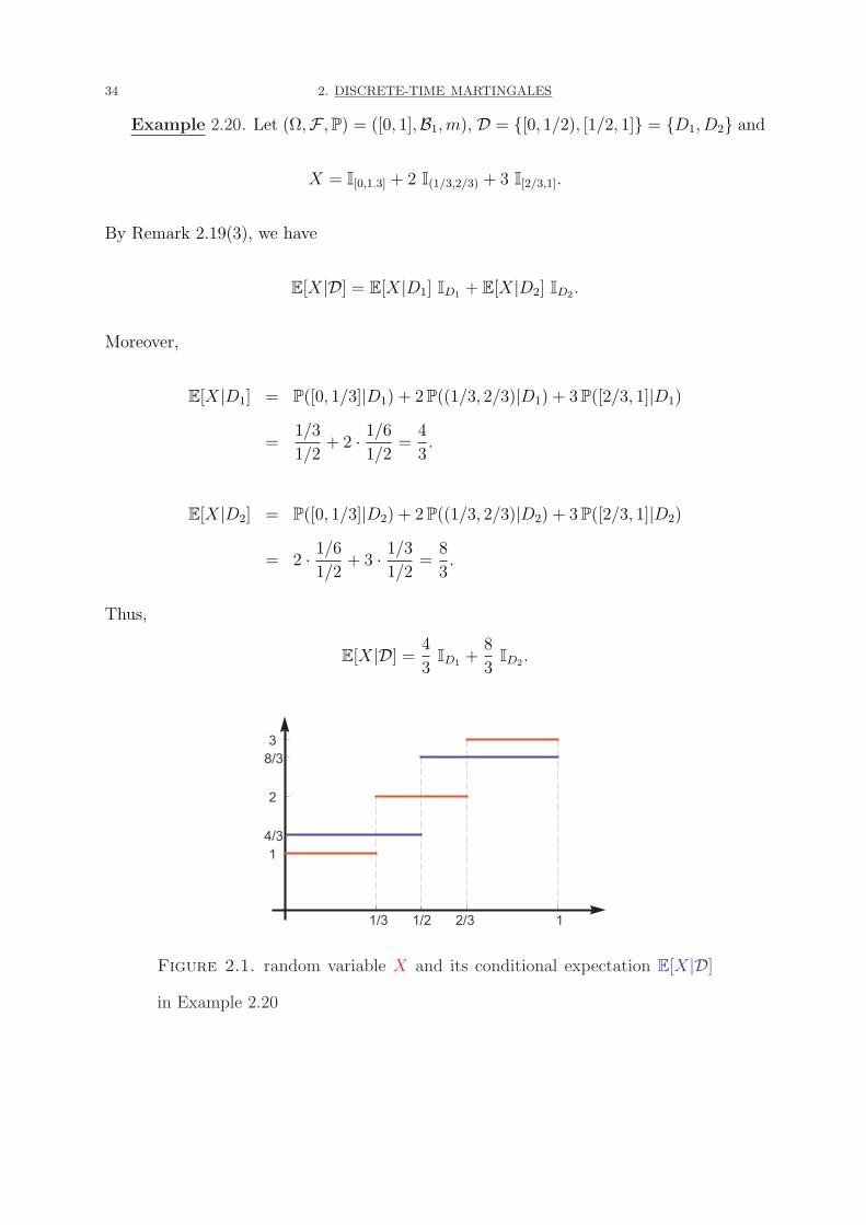
Example 2.20. Let (Ω,F , P) = ([0, 1],B1,m), D = {[0, 1/2), [1/2, 1]} = {D1, D2} and

X = I[0,1.3] + 2 I(1/3,2/3) + 3 I[2/3,1].

By Remark 2.19(3), we have

E[X|D] = E[X|D1] ID1 + E[X|D2] ID2 .

Moreover,

E[X|D1] = P([0, 1/3]|D1) + 2 P((1/3, 2/3)|D1) + 3 P([2/3, 1]|D1)

=1/3

1/2+ 2 · 1/6

1/2=

4

3.

E[X|D2] = P([0, 1/3]|D2) + 2 P((1/3, 2/3)|D2) + 3 P([2/3, 1]|D2)

= 2 · 1/6

1/2+ 3 · 1/3

1/2=

8

3.

Thus,

E[X|D] =4

3ID1 +

8

3ID2 .

1/3 1/2 2/3 1

1

2

38/3

4/3

Figure 2.1. random variable X and its conditional expectation E[X|D]

in Example 2.20


�� X simple random variable � case, � X positive random

variable, �� random variable � case, construct �� Section 1.3 �

construct expectation ��, �� .

2.1.4. Conditional expectation with respect t0 σ-algebra . ��: ��

�� Y discrete random variable. � Y continuous random variable, ��

�� uncountable ��?

Now, for G ⊆ F : subalgebra and X is a nonnegative random variable. How to define

E[X|G]?

��? ��

�� random variable X ��. �, ��

�, ��.

Definition 2.21. The conditional expectation of X with respect to G is a nonnegative

random variable denoted by E[X|G] or E[X|G](ω), such that

(i) E[X|G] is G-measurable.1

(ii) For all A ∈ G, ∫A

E[X|G] dP =

∫A

X dP.2

�� information �. ��, σ-algebra �� information,

E[X|G] �� G �� information ��. �� (i) ��

� G ��. �� (ii) ��.

1��“��”. �� {E[X|G] ≤ C} ∈ G for all C. ��

��.

2� G ��, random variable X �� E[X|G]��.


��: �� X and G, � �� well-defined? ��

��?

��: Radon-Nikodym Theorem. ��

�� . ��!��, ��!��

��. ��.

Remark 2.22. The conditional expectation exists and is unique for all X and G up

to some P-null set due to Radon-Nikodym theorem.

Example 2.23. (1) Consider a probability space ([0, 1],B1,m). Let X be uni-

formly distributed on [0, 1] and let

G = σ

({0 ≤ X <

1

2

},

{1

2≤ X ≤ 1

}).

We have two different method to get the desired conditional expectation.

Method 1: Using the decomposition of sample space. Then

E[X|G] = E

[X

∣∣∣∣{

0 ≤ X <1

2

}]I{0≤X< 1

2} + E

[X

∣∣∣∣{

1

2≤ X ≤ 1

}]I{ 1

2≤X≤1}.

Since

P

[A

∣∣∣∣{

0 ≤ X <1

2

}]=

P

(A ∩

{0 ≤ X <

1

2

})P

({0 ≤ X <

1

2

}) ,

we have

E [X |{0 ≤ X < 1/2} ] =

∫[0,1]

X dP (· ∩ {0 ≤ X < 1/2})P ({0 ≤ X < 1/2})

=1

P ({0 ≤ X < 1/2})∫

[0,1]

XI{0≤X<1/2} dP

=1

1/2

∫ 1/2

0

x dx = x2∣∣1/2

x=0=

1

4.


Similarly, we have

E [X |{1/2 ≤ X < 1} ] =1

P ({1/2 ≤ X < 1})∫

[0,1]

XI{1/2≤X<1} dP

=1

1/2

∫ 1

1/2

x dx = x2∣∣1x=1/2

=3

4.

Method 2: Using the definition of condition expectation: By Definition 2.21 (i),

we see that

E[X|G] = c1 I{0≤X< 12} + c2 I{ 1

2≤X≤1}.

For A = {0 ≤ X < 12},

∫A

E[X|G] dP = c1P({0 ≤ X <1

2}) =

c1

2,

∫A

X dP =

∫ 1/2

0

x dx =1

2x2

∣∣1/2

x=0=

1

8.

By Definition 2.21 (ii), we see that

c1

2=

1

8.

Hence, c1 = 1/4. Similarly, we can get c2 = 3/4.

Thus,

E[X|G] =1

4I{0≤X< 1

2} +

3

4I{ 1

2≤X≤1}.

(2) Consider a probability space ([0, 1],B1,m). Let X be a random variable with

probability density function f(x) = 2x. Let

G = σ

({0 ≤ X <

1

3

},

{1

3≤ X <

2

3

},

{2

3≤ X ≤ 1

}).

Using a similar argument as above, we have

E[X|G] =2

9I{0≤X< 1

3} +

14

27I{ 1

3≤X< 2

3} +

38

45I{ 2

3≤X≤1}.


How about the general case?

Let X be a general random variable. As the same as the integrability argument in

Chapter 1, consider

X = X+ − X−,

where X+ = X ∨ 0, X− = (−X) ∨ 0.

Assumption. min{E[X+], E[X−]} < ∞.

Definition 2.24. The conditional expectation E[X|G], or E[X|G](ω), of any random

variable with respect to the σ-algebra G, is defined by

E[X|G] = E[X+|G] − E[X−|G],

if min{E[X+|G], E[X−|G]} < ∞ P-a.s. On the set of sample points for which E[X+|G] =

E[X−|G] = ∞, E[X+|G] − E[X−|G] is given by an arbitrary value.

�� conditional probability, �� conditional probability ��

conditional expectation. � ��"��: �� conditional expectation,

�� conditional expectation �� conditional probability.

��, ��

E[X] =

∫Ω

X dP.

Take X = IA, then

E[IA] =

∫Ω

IA dP =

∫A

dP = P(A).

�� X �� IA ��, �� conditional

probability.


Definition 2.25. Let B ∈ F . The conditional probability of B with respect to G is

defined by

P(B|G) = E[IB|G].

Proposition 2.26. (1) If X ≡ C P-a.s., then E[X|G] = C P-a.s.

(2) If X ≤ Y P-a.s., then E[X|G] ≤ E[Y |G] P-a.s.

(3) |E[X|G]| ≤ E[|X||G] P-a.s.

(4) For constants a,b with aE[X] + bE[Y ] < ∞, then

E[aX + bY ] = aE[X] + bE[Y ].

(5) Consider the trivial σ-algebra F∗ = {∅, Ω}. Then

E[X|F∗] = E[X], P − a.s.

(6) If X is G-measurable, then E[X|G] = X.

(7) E[E[X|G]] = E[X].

(8) (Tower property) If G1 ⊂ G2, then

E[E[X|G1]|G2] = E[X|G1] = E[E[X|G2]|G1].

(9) Let Y be G-measurable with E|X| < ∞, E|XY | < ∞. Then

E[XY |G] = Y E[X|G], P − a.s.

Proof. (1), (2), (4), (5), (6) are easy by definition of conditional expectation.

(3) Consider X = X+ − X−.

(7) By the second assertion of Definition 2.21, let A = Ω, we have

E[E[X|G]] =

∫Ω

E[X|G] dP =

∫Ω

X dP = E[X]


(8) (i) Since E[X|G1] is G1-measurable and G1 ⊂ G2, E[X|G1] is G2-measurable. By

the above statement (6), we have E[E[X|G1]|G2] = E[X|G1].

(ii) Clearly, E[E[X|G2]|G1] is G1-measurable. Moreover, for A ∈ G1,

∫A

E[E[X|G2]|G1] dP =

∫A

E[X|G2] dP =A∈G2

∫A

X dP

=

∫A

E[X|G1] dP.

(9) This proof is a little bit complicated. We give here only the sketch of the proof.

Step 1: Consider first the case Y is a G-measurable indicator function, i.e.,

Y = IA for A ∈ G. It is easy to prove this due to Definition 2.21.

Step 2: Using the linearity property (4) to prove the case where Y is a G-

measurable simple random variable.

Step 3: Using a sequence of G-measurable simple random variables to ap-

proach the positive G-measurable random variable Y .

Step 4: For the general case, consider Y = Y + − Y −.

�

Theorem 2.27. Let (Xn) be a sequence of random variables.

(1) (Conditional Dominated Convergence Theorem) If |Xn| ≤ X, E|X| < ∞, and

Xn −→ X P-a.s., then

E[Xn|G] −→ E[X|G], P − a, s.

(2) (Conditional Monotone Convergence Theorem)

(i) If Xn ≥ Y , E[Y ] > −∞, and Xn ↗ X P-a.s., then

E[Xn|G] ↗ E[X|G], P − a, s.


(ii) If Xn ≤ Y , E[Y ] < ∞, and Xn ↘ X P-a.s., then

E[Xn|G] ↘ E[X|G], P − a, s.

(3) (Conditional Fatou’s Lemma)

(i) If Xn ≥ Y and E[Y ] > −∞, then

E[lim infn

Xn|G] ≤ lim infn

E[Xn|G].

(ii) If Xn ≤ Y and E[Y ] < ∞, then

lim supn

E[Xn|G] ≤ E[lim supn

Xn|G].

(4) If Xn ≥ 0, then

E

[∑n

Xn

∣∣∣∣∣G]

=∑

n

E[Xn|G].

(5) (Conditional Jensen’s inequality) If ϕ is a convex function on R and E[X] < ∞,

E[ϕ(X)] < ∞, then

ϕ (E[X|G]) ≤ E[ϕ(X)|G].

Remark 2.28. Denote

σ(Y ) = {{ω : Y (ω) ∈ B} : B ∈ B1} = σ({Y ≤ r}) : r ∈ R.

Then

E[X|Y ]︸︷︷︸Notation 2.9

= E[X|σ(Y )]︸︷︷︸Definition 2.21

.

Proposition 2.29. If Y and a σ-algebra G are independent3,

E[Y |G] = E[Y ].

3(1) Two σ-algebras G1 and G2 are independent if for every Ai ∈ Gi, A1 and A2 are independent.

(2) We say that a random variable Y and a σ-algebra G are independent if σ(Y ) and G are independent.


Exercise

(1) Consider a probability space (Ω,F , P) with Ω = {1, 2, 3, 4}, F = σ({1}, {2}, {3}, {4}),and

P({1}) =1

6, P({2}) =

1

3, P({3}) =

1

4, P({4}) =

1

4.

Define three random variables, X, Y and Z, by

X(1) = 1, X(2) = 1, X(3) = −1, X(4) = −1,

Y (1) = 1, Y (2) = −1, Y (3) = 1, Y (4) = −1,

and Z = X + Y .

(a) List the sets in σ(X).

(b) Determine E[Y |X] and E[Z|X].

(c) Find E[Z|X] = E[Y |X].

(d) Let B = {1, 2, 4}. For A ∈ F , find P(A|B).

(e) Let

W = I{1,2,4} + 2I{3},

find E[X|W = 1], E[X|W = 2], and E[X|W ].

(2) Consider the probability space ([0, 1],B1,m).

(a) Suppose X is uniformly distributed on [0, 1] and

G = σ({0 ≤ X ≤ 1/2}, {1/2 < X ≤ 2/3}, {2/3 < X ≤ 1}).

Find E[X|G].

(b) Suppose the probability density function of Y is f(y) = 2y on [0, 1] and

G = σ({0 ≤ Y ≤ 1/2}, {1/2 < Y ≤ 2/3}, {2/3 < Y ≤ 1}).


Find E[Y |G].

(3) Consider the probability space ([0, 1],B1,m).

(a) Let

X(ω) = 3ω2, Y (ω) =

⎧⎪⎨⎪⎩

2, if 0 ≤ ω < 1/2,

ω, if 1/2 ≤ ω ≤ 1.

Find E[X|Y ] and E[X2|Y ].

(b) Let X and Y be random variables with joint density function

fX,Y (x, y) =

⎧⎪⎨⎪⎩

3

2(x2 + y2), if x, y ∈ [0, 1],

0, otherwise.

Find E[X|Y ] and E[X2|Y ].

(4) Let X and Y be integrable random variables on a probability space (Ω,F , P).

Then we can decompose Y into

Y = Y1 + Y2,

where Y1 = E[Y |X] and Y2 = Y − E[Y |X].

(a) Show that Y2 and X are uncorrelated.

(b) More general, show that Y2 is uncorrelated with every σ(X)-measurable ran-

dom variable.

Hint: For every σ(X)-measurable random variable W , there exists a func-

tion g such that W = g(X).

(5) Let X1, X2, ..., Xn be a sequence of independent identically distributed random

variables and let

Sn = X1 + X2 + · · · + Xn.


Suppose P(X1 = 1) = p = 1 − P(Xi = 0) for some 0 < p < 1. Compute the

value of P(X1 = 1|Sn = k) for k = 0, 1, 2, ..., n and the conditional expectation

E[X1|Sn = k].

2.2. Discrete-time martingales

Let (Ω,F , P) be a probability space.

Definition 2.30. (1) A sequence of σ-algebra (Fn)n≥1 is called a filtration if Fn ⊆Fn+1 for all n ≥ 1.

(2) A probability space (Ω,F , P) with filtration F = (Fn) is called a filtered probability space,

and is denoted by (Ω,F , F, P) or (Ω,F , (Fn), P).

Example 2.31. Let Ω = N = {1, 2, ..., n} and let F = the collection of all subsets of

Ω. Set

F0 = {, Ω}

F1 = σ({1})

F2 = σ({1}, {2})...

Fn = σ({1}, {2}, ..., {n})...

Then (Fn) is a filtration.

2.2. DISCRETE-TIME MARTINGALES 45

Definition 2.32. Let (Xn)n≥1 be a sequence of random variables and (Fn)n≥1 is a

filtration. We say (Xn,Fn) is a martingale (��, or say (Xn) is a martingale with

respect to (Fn), (Xn) is an (Fn)-martingale) if

(a) Xn ∈ Fn for all n, i.e., (Xn) is (Fn)-adapted;

(b) E|Xn| < ∞ for all n;

(c) Xn = E(Xn+1|Fn), P-a.s. for all n.

Remark 2.33. The condition (c) in Definition 2.32 is equivalent to

(c′) Xn = E(Xm|Fn) for all m > n.

(c′′)

∫A

Xn dP =

∫A

Xm dP for all A ∈ Fn and for all m > n.

Example 2.34. (1) Let (ξn) be a sequence of independent and identically dis-

tributed random variables with E|ξn| < ∞ and E(ξn) = 0. Define

Xn =n∑

i=1

ξi and Fn = σ(ξ1, · · · , ξn) = σ(X1, · · · , Xn)4.

Then

(a) Since ξ1, ξ2, ..., ξn ∈ Fn, Xn ∈ Fn for all n.

(b) E|Xn| = E

∣∣∣∣∣n∑

i=1

ξi

∣∣∣∣∣ ≤n∑

i=1

E|ξi| < ∞;

4Proof of σ(ξ1, · · · , ξn) = σ(X1, · · · , Xn):

(a) Since Xn =n∑

i=1

ξi, we have Xn ∈ σ(ξ1, · · · , ξn). Thus,

σ(X1, · · · , Xn) ⊆ σ(ξ1, · · · , ξn).

(b) Since ξn = Xn − Xn−1, we have ξn ∈ σ(Xn−1, Xn) ⊆ σ(X1, · · · , Xn). Thus,

σ(ξ1, · · · , ξn) ⊆ σ(X1, · · · , Xn).


(c) Due to the definition of Xn, independence of (ξn) and Lemma 2.29, we have

E[Xn+1|Fn] = E[Xn + ξn+1|Fn] = Xn + E[ξn+1|Fn]

= Xn + E[ξn+1] = Xn, P − a.s.

Thus, (Xn,Fn) is a martingale.

(2) Let (ξn) be a sequence of independent strictly positive random variables with

Eξn = 1 for all n. Define

Xn =n∏

i=1

ξi,

Fn = σ(ξ1, ξ2, ..., ξn).

Then

(a) Since ξ1, ξ2, ..., ξn ∈ Fn, this implies that Xn ∈ Fn for all n.

(b) Since ξi > 0 for all i,

E|Xn| = E

(n∏

i=1

ξi

)=

n∏i=1

E[ξi] = 1 < ∞.

(c) Due to the definition of Xn, independence of (ξn) and Lemma 2.29, we have

E[Xn+1|Fn] = E[Xnξn+1|Fn] = XnE[ξn+1|Fn]

= XnE[ξn+1] = Xn.

Thus, (Xn,Fn) is a martingale.

(3) Let X be a random variable with E|X| < ∞ and (Fn) is a filtration. Define

Xn = E(X|Fn) for all n. Then (Xn,Fn) is a martingale.

Remark 2.35. The choices of P and (Fn) are important.


Lemma 2.36. If (Xn) is an (Fn)-martingale, then

E(Xn) = E(Xn−1) = · · · = E[X0].

Definition 2.37. (1) (Xn) is an (Fn)-submartingale (��, �, �) if (a) +

(b) +

(d) Xn ≤ E(Xn+1|Fn) for all n P -a.s.

(2) (Xn) is an (Fn)-supermartingale (!�, �, ) if (a) + (b) +

(e) Xn ≥ E(Xn+1|Fn) for all n P -a.s.

Remark 2.38. (1) Xn ≤ E(Xn+1|Fn) P-a.s. for all n

⇐⇒ Xn ≤ E(Xm|Fn) for all m > n P -a.s.

⇐⇒∫

A

Xn dP ≤∫

A

Xm dP for all m > n and for all A ∈ Fn.

(2) Xn ≥ E(Xn+1|Fn) P-a.s. for all n

⇐⇒ Xn ≥ E(Xm|Fn) for all m > n P -a.s.

⇐⇒∫

A

Xn dP ≥∫

A

Xm dP for all m > n and for all A ∈ Fn.

(3) (Xn,Fn) is a submartingale

⇐⇒ (−Xn,Fn) is a supermartingale.

(4) (Xn,Fn) is a martingale

⇐⇒ (Xn,Fn) is a submartingale and supermartingale.

Theorem 2.39. Let (Xn,Fn) be a submartingale and let ϕ be an increasing convex

function defined on R. If ϕ(Xn) is integrable for all n, then (ϕ(Xn)) is a submartingale

w.r.t. Fn.

Proof. Since ϕ is increasing and

E[Xn+1|Fn] ≥ Xn P − a.s.,


we have

ϕ(Xn) ≤ ϕ (E[Xn+1|Fn]) ≤ E[ϕ(Xn+1)|Fn] (conditional Jensen’s inequality).

This implies that (ϕ(Xn)) is a submartingale. �

Remark 2.40. (1) If (Xn) is a martingale and ϕ is a convex function defined on

R, then ϕ(Xn) is a submartingale.

(2) If (Xn) is a martingale and ϕ is a concave function defined on R, then ϕ(Xn) is

a supermartingale.

Corollary 2.41. If (Xn,Fn) is a submartingale, then (X+n ,Fn) is a submartingale.

Corollary 2.42. If (Xn,Fn) is a martingale, then

(1) If Xn ∈ Lp, (|Xn|p,Fn) is a submartingale for 1 < p < ∞.

(2) (|Xn|,Fn) is a submartingale.

(3) (|Xn| log+ |Xn|,Fn) is a submartingale, where log+ x = max{log x, 0} for x > 0.

Proof. |x|p, |x|, and |x| log+ |x| are convex. �

Corollary 2.43. If (Xn,Fn) is a supermartingale, (Xn∧A) is a supermartingale with

a constant A.

Proof. Exercise. �

Example 2.44. (1) Let (ξn) be independent random variables with E|ξn| < ∞and E(ξn) ≥ 0. Define

Xn =n∑

i=1

ξi and Fn = σ(ξ1, · · · , ξn).


Then

E[Xn+1|Fn] = E[Xn + ξn+1|Fn] = Xn + E[ξn+1|Fn]

= Xn + E[ξn+1] ≥ Xn, P − a.s.

This implies that (Xn,Fn) is a submartingale.

(2) (Xn,Fn) is a martingale, then (exp(Xn),Fn) is a submartingale.

(3) Let (ξn) be a sequence of independent random variables with 0 ≤ ξn ≤ 1 for all

n. Define

Xn =n∏

i=1

ξi.

Then

E[Xn+1|Fn] = XnE[ξn+1|Fn] = XnE[ξn] ≤ Xn.

Thus, (Xn,Fn) is a supermartingale.

Exercise

(1) Let ξ1, ξ2, ... be a sequence of coin tosses and let Fn be the σ-algebra generated

by ξ1, ξ2, ..., ξn. For each of the following events find the smallest n such that

the even belong to Fn.

A = { the first occurence of heads is preceeded by no more than 10 tails },B = { there is at least 1 head in the sequence ξ1, ξ2, ...},C = { the first 100 tosses produce the same outcome },D = { there are no more than 2 heads and 2 tails among the first 5 tosses }.

(2) Let X be a random variable with E|X| < ∞. Define Xn = E[X| Fn] for all n.

Prove that (Xn) is an (Fn)-martingale.


(3) Let X1 and Y1 be independent and identically distributed random variables with

P(X1 = 1) = P(X1 = −1) = 1/2. Moreover, define

Z =

⎧⎪⎨⎪⎩

1, if X1 + Y1 = 0,

−1, if X1 + Y1 = 0.

Set X2 = X1 + Z and Y2 = Y1 + Z. Show that (Xi)i=1,2 and (Yi)i=1,2 are

martingales, but (Xi + Yi)i=1,2 is not.

(4) Let (Xn) be a sequence of random variables defined by

Xn = ξ1 + ξ2 + · · · + ξn,

where ξ1, ξ2, ... is a sequence of independent identically distributed random

variables such that

P(ξn = 1) = P(ξn = −1) =1

2.

(a) Show that X2n − n is a martingale with respect to the filtration Fn =

σ(ξ1, ξ2, ..., ξn).

(b) Show that the stochastic process (Yn) defined by

Yn = (−1)n cos(πXn)

is a martingale with respect to (Fn)

(5) Let (ξn) be a sequence of independent identically distributed Bernoulli random

variables with generating function M(t) = E[exp(tξ1)] < ∞ for t = 0 and let

Xn =n∑

i=1

ξi. Prove that the sequence (Zn) with

Zn = exp(tXn)/Mn(t)

is a martingale.

2.3. MARTINGALE TRANSFORMS AND DOOB DECOMPOSITION 51

(6) Let X0 = 0 and for k ∈ N,

P(Xk = 1|Xk−1 = 0) = P(Xk = −1|Xk−1 = 0) =1

2k, P(Xk = 0|Xk−1 = 0) = 1 − 1

k

and

P(Xk = k · Xk−1|Xk−1 = 0) =1

kP(Xk = 0|Xk−1 = 0) = 1 − 1

k.

Show that (Xn) is a martingale with respect to (Fn), where Fn = σ(X0, X1, ..., Xn).

2.3. Martingale transforms and Doob decomposition

2.3.1. Martingale transforms. Consider a filtered probability space (Ω,F , (Fn), P).

Definition 2.45. If Mn ∈ Fn−1 for all n, we say that the stochastic process (Mn) is

an (Fn)-predictable process.

Definition 2.46. (1) Let (Xn,Fn) be a stochastic process and let M = (Mn,Fn−1)

be a predictable process, then the stochastic process

(M · X)n = M0X0 +n∑

i=1

Mi(Xi − Xi−1)

is called the transform of X by M .

(2) If, in addition, X is a martingale, we say that M · X is a martingale transform.

Theorem 2.47 (Martingale transformation theorem). Let (Mn) be a sequence of

bounded random variables.

(1) If (Xn,FXn ) is a supermartingale and (Mn) is a sequence of (Fn)-predictable

nonnegative random variables, then ((M · X)n,FXn ) is a supermartingale.

(2) If (Xn,FXn ) is a submartingale and (Mn) is a sequence of (Fn)-predictable non-

negative random variables, then ((M · X)n,FXn ) is a submartingale.


(3) If (Xn,FXn ) is a martingale and (Mn) is a sequence of (Fn)-predictable random

variables, then ((M · X)n,FXn ) is a martingale.

Proof. (2) Since

(M · X)n = M1X1 +n∑

i=1

Mi(Xi − Xi−1)

= M1X1 +n∑

i=1

Mi(Xi − E[Xi|Fi−1])︸︷︷︸martingale part

+n∑

i=1

Mi(E[Xi|Fi−1] − Xi−1)︸︷︷︸increasing process part

,

we see that (M ·X)n is a submartingale. (�� Theorem 2.50 ��.

��"��) �

2.3.2. Doob decomposition.

Definition 2.48. A sequence of random variables (Zn) is called an increasing process

if

(1) Z1 = 0 and Zn ≤ Zn+1 for all n ≥ 1.

(2) E(Zn) < ∞ for all n.

Example 2.49. (1) Zn = n − 1 for all n, then (Zn) is an increasing process.

(2) Zn = (n−1)X, where X is a nonnegative random variable with E(X) < ∞, then

(Zn) is an increasing process.

(3) Zn ∼ N (0, n−1) for all n and (Zn) are independent, then (Zn) is not an increasing

process.

Theorem 2.50 (Doob decomposition). Any submartingale (Xn,Fn) can be written as

Xn = Yn + Zn, (2.3)

2.3. MARTINGALE TRANSFORMS AND DOOB DECOMPOSITION 53

where (Yn,Fn) is a martingale and (Zn) is an increasing predictable process.

Proof. Let

Y1 = X1,

Yn = X1 +n∑

i=2

[Xi − E(Xi|Fi−1)], for n ≥ 2.

Claim: (1) (Yn) is a martingale with respect to (Fn).

(2) Zn := Xn − Yn is an increasing process.

(1) By definition

E[Yn+1|Fn] = E[X1 +n+1∑i=2

[Xi − E(Xi|Fi−1)]|Fn]

= X1 +n∑

i=2

[Xi − E(Xi|Fi−1)]︸︷︷︸(i)

+ E[Xn+1 − E[Xn+1|Fn]|Fn]︸︷︷︸(ii)

Clearly,

(i) = Yn,

(ii) = E[Xn+1|Fn] − E[Xn+1|Fn]|Fn] = E[Xn+1|Fn] − E[Xn+1|Fn] = 0.

Thus, (Yn) is a martingale.

(2) Z1 = X1 − Y1 = 0. For n ≥ 2, we have

Zn = Xn − Yn = Xn −(

X1 +n∑

i=1

(Xi − E[Xi|Fi−1])

).


Thus,

Zn+1 − Zn =

(Xn+1 −

(X1 +

n+1∑i=1


))

−(

Xn −(

X1 +n∑

i=1


))

= (Xn+1 − Xn) − (Xn+1 − E[Xn+1|Fn])

= E[Xn+1|Fn] − Xn ≥ 0,

since (Xn) is a submartingale.

(3) Moreover, we have

Zn = Xn − X1 −n∑

i=1


= E[Xn|Fn−1] − X1 −n−1∑i=1

(Xi − E[Xi|Fi−1]) ∈ Fn−1.

Thus, (Zn) is an (Fn)-predictable process.

�

Remark 2.51. (1) The decomposition (2.3) is unique.

(2) An increasing predictable Z in (2.3) is called a compensator of the submartingale

X.

Discrete-Time Martingalesocw.nctu.edu.tw/upload/classbfs120912252641448.pdf · CHAPTER 2...

Documents

Transcript of Discrete-Time Martingalesocw.nctu.edu.tw/upload/classbfs120912252641448.pdf · CHAPTER 2...