Introduction to the Discrete-Time Fourier Transform and ...

Introduction to the Discrete-TimeFourier Transform and the DFT

C.S. Ramalingam

Department of Electrical EngineeringIIT Madras

C.S. Ramalingam (EE Dept., IIT Madras) Introduction to DTFT/DFT 1 / 37

The Discrete-Time Fourier Transform

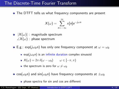
The DTFT tells us what frequency components are present

X (ω) =∞∑

n=−∞x [n]e−jωn

|X (ω)| : magnitude spectrum∠X (ω) : phase spectrum

E.g.: exp(jω0n) has only one frequency component at ω = ω0

exp(jω0n) is an infinite duration complex sinusoid

X (ω) = 2π δ(ω − ω0) ω ∈ [−π, π)

the spectrum is zero for ω 6= ω0

cos(ω0n) and sin(ω0n) have frequency components at ±ω0

phase spectra for sin and cos are different


The Discrete-Time Fourier Transform

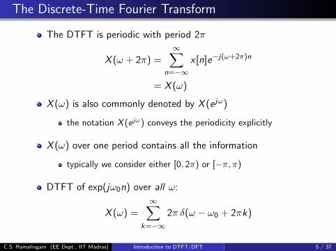
The DTFT is periodic with period 2π

X (ω + 2π) =∞∑

n=−∞x [n]e−j(ω+2π)n

= X (ω)

X (ω) is also commonly denoted by X (e jω)

the notation X (e jω) conveys the periodicity explicitly

X (ω) over one period contains all the information

typically we consider either [0, 2π) or [−π, π)

DTFT of exp(jω0n) over all ω:

X (ω) =∞∑

k=−∞2π δ(ω − ω0 + 2πk)


Inverse DTFT

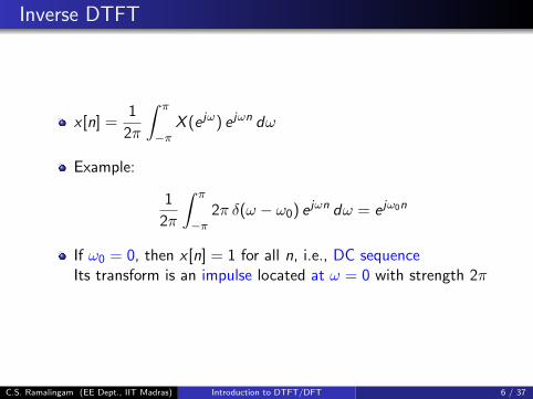
x [n] =1

2π

∫ π

−πX (e jω) e jωn dω

Example:

1

2π

∫ π

−π2π δ(ω − ω0) e jωn dω = e jω0n

If ω0 = 0, then x [n] = 1 for all n, i.e., DC sequenceIts transform is an impulse located at ω = 0 with strength 2π


Convolution-Multiplication Property

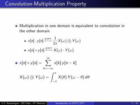
Multiplication in one domain is equivalent to convolution inthe other domain

x [n] · y [n]DTFT←→ 1

2πX (ω)©∗ Y (ω)

x [n] ∗ y [n]DTFT←→ X (ω) · Y (ω)

x [n] ∗ y [n] =∞∑

k=−∞x [k] y [n − k]

X (ω)©∗ Y (ω) =

∫ π

−πX (θ) Y (ω − θ) dθ


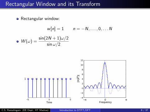
Rectangular Window and its Transform

Rectangular window:

w [n] = 1 n = −N, . . . , 0, . . .N

W (ω) =sin(2N + 1)ω/2

sinω/2

−5 0 5Time

−π

1

−4

−2

0

2

4

6

8

10

12

Frequency

|X(e

jω)|

π0


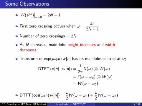
Some Observations

W (e jω)∣∣ω=0

= 2N + 1

First zero crossing occurs when ω =2π

2N + 1

Number of zero crossings = 2N

As N increases, main lobe height increases and widthdecreases

Transform of exp(jω0n) w [n] has its mainlobe centred at ω0

DTFT (x [n] · w [n]) =1

2πX (ω)©∗ W (ω)

= δ(ω − ω0)©∗ W (ω)

= W (ω − ω0)

DTFT (cos(ω0n) w [n]) =1

2W (ω − ω0) +

1

2W (ω + ω0)


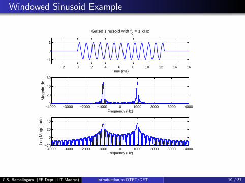
Windowed Sinusoid Example

−2 0 2 4 6 8 10 12 14 16

−1

0

1

Time (ms)

Gated sinusoid with f0 = 1 kHz

−4000 −3000 −2000 −1000 0 1000 2000 3000 40000

20

40

60

Frequency (Hz)

Mag

nitu

de

−4000 −3000 −2000 −1000 0 1000 2000 3000 4000−20

0

20

40

Frequency (Hz)

Log

Mag

nitu

de


Single Real Sinusoid Frequency Estimation

f0 is estimated from peak location

In general, the peaks are not exactly at ±f0

This is because of sidelobe interference

If f0 is closer to DC

sidelobe interference increases

shifts peak further away from true location

Interference is least when sinusoidal frequency is at fs/4


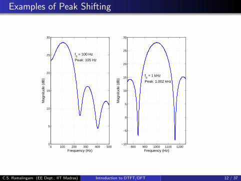
Examples of Peak Shifting

0 100 200 300 400 5000

5

10

15

20

25

30

f0 = 100 Hz

Peak: 105 Hz

Frequency (Hz)

Mag

nitu

de (

dB)

800 900 1000 1100 1200−10

−5

0

5

10

15

20

25

30

Frequency (Hz)

Mag

nitu

de (

dB)

f0 = 1 kHz

Peak: 1.002 kHz


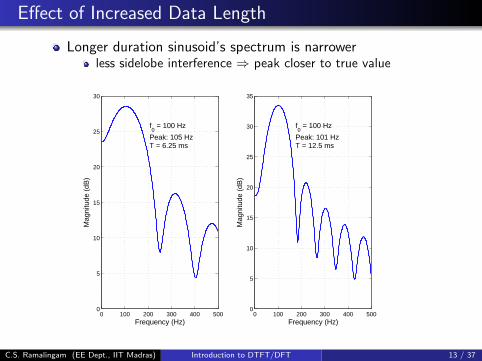
Effect of Increased Data Length

Longer duration sinusoid’s spectrum is narrowerless sidelobe interference ⇒ peak closer to true value

0 100 200 300 400 5000

5

10

15

20

25

30

f0 = 100 Hz

Peak: 105 HzT = 6.25 ms

Frequency (Hz)

Mag

nitu

de (

dB)

0 100 200 300 400 5000

5

10

15

20

25

30

35

Frequency (Hz)

Mag

nitu

de (

dB)

f0 = 100 Hz

Peak: 101 HzT = 12.5 ms


Use of Data Windows

Useful for data containing sinusoids

Sidelobes of a stronger sinusoid will mask the main lobe of anearby weak sinusoid

We multiply x [n] by data window w [n] before computing theDTFT

if we merely truncate a signal, it is equivalent to applying arectangular window

Why consider non-rectangular windows?

sidelobes fall of faster

nearby weaker sinusoid becomes more visible

price paid: main lobe of each sinusoid broadens

two close peaks may merge into one


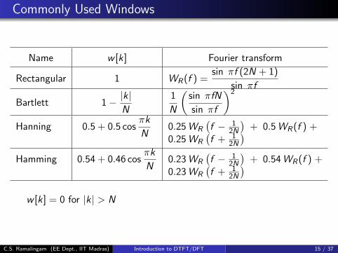
Commonly Used Windows

Name w [k] Fourier transform

Rectangular 1 WR(f ) =sin πf (2N + 1)

sin πf

Bartlett 1− |k |N

1

N

(sin πfN

sin πf

)2

Hanning 0.5 + 0.5 cosπk

N0.25 WR

(f − 1

2N

)+ 0.5 WR(f ) +

0.25 WR

(f + 1

2N

)Hamming 0.54 + 0.46 cos

πk

N0.23 WR

(f − 1

2N

)+ 0.54 WR(f ) +

0.23 WR

(f + 1

2N

)w [k] = 0 for |k | > N


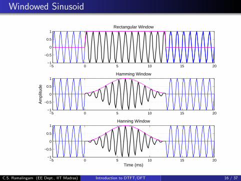
Windowed Sinusoid

−5 0 5 10 15 20−1

−0.5

0

0.5

1Rectangular Window

−5 0 5 10 15 20−1

−0.5

0

0.5

1

Am

plitu

de

Hamming Window

−5 0 5 10 15 20−1

−0.5

0

0.5

1

Time (ms)

Hanning Window


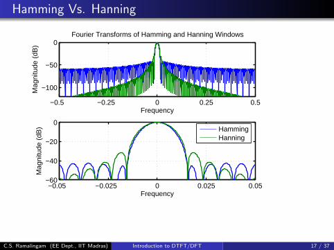
Hamming Vs. Hanning

−0.05 −0.025 0 0.025 0.05−60

−40

−20

0

Frequency

Mag

nitu

de (

dB)

−0.5 −0.25 0 0.25 0.5

−100

−50

0Fourier Transforms of Hamming and Hanning Windows

Frequency

Mag

nitu

de (

dB)

HammingHanning


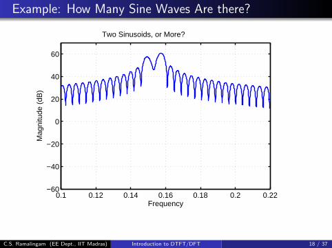
Example: How Many Sine Waves Are there?

0.1 0.12 0.14 0.16 0.18 0.2 0.22−60

−40

−20

0

20

40

60

Frequency

Mag

nitu

de (

dB)

Two Sinusoids, or More?


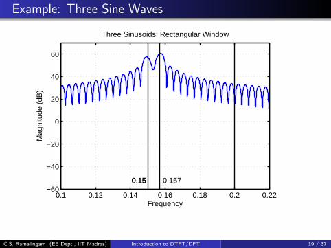
Example: Three Sine Waves

0.1 0.12 0.14 0.16 0.18 0.2 0.22−60

−40

−20

0

20

40

60

Frequency

Mag

nitu

de (

dB)

Three Sinusoids: Rectangular Window

0.150.15 0.157


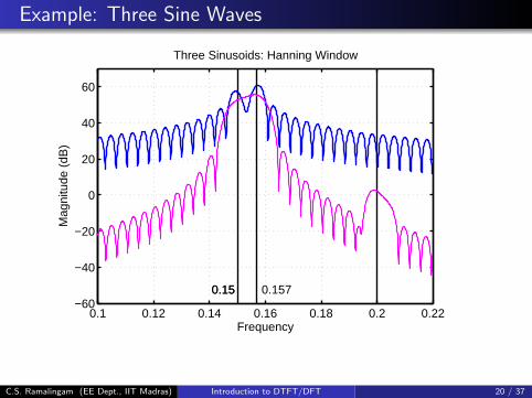
Example: Three Sine Waves

0.1 0.12 0.14 0.16 0.18 0.2 0.22−60

−40

−20

0

20

40

60

Frequency

Mag

nitu

de (

dB)

Three Sinusoids: Hanning Window

0.150.15 0.157


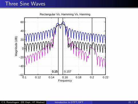
Three Sine Waves

0.1 0.12 0.14 0.16 0.18 0.2 0.22−60

−40

−20

0

20

40

60

Frequency

Mag

nitu

de (

dB)

Rectangular Vs. Hamming Vs. Hanning

0.150.15 0.157


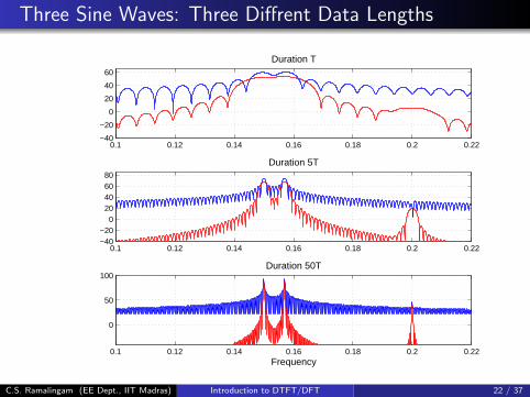
Three Sine Waves: Three Diffrent Data Lengths

0.1 0.12 0.14 0.16 0.18 0.2 0.22−40

−20

0

20

40

60

Duration T

0.1 0.12 0.14 0.16 0.18 0.2 0.22−40−20

020406080

Duration 5T

0.1 0.12 0.14 0.16 0.18 0.2 0.22

0

50

100

Frequency

Duration 50T


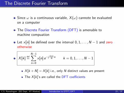
The Discrete Fourier Transform

Since ω is a continuous variable, X (ω) cannote be evaluatedon a computer

The Discrete Fourier Transform (DFT) is amenable tomachine compuation

Let x [n] be defined over the interval 0, 1, . . . ,N − 1 and zerootherwise

X [k]def=

N−1∑n=0

x [n] e−j 2πkN

n k = 0, 1, . . . ,N − 1

X [k + N] = X [k] i.e., only N distinct values are present

The X [k]’s are called the DFT coefficients


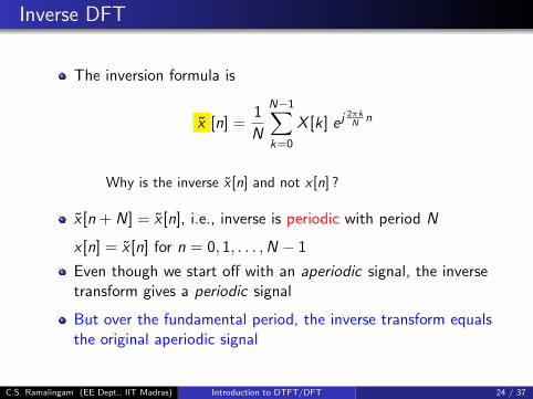
Inverse DFT

The inversion formula is

x [n] =1

N

N−1∑k=0

X [k] e j 2πkN

n

Why is the inverse x [n] and not x [n] ?

x [n + N] = x [n], i.e., inverse is periodic with period N

x [n] = x [n] for n = 0, 1, . . . ,N − 1

Even though we start off with an aperiodic signal, the inversetransform gives a periodic signal

But over the fundamental period, the inverse transform equalsthe original aperiodic signal


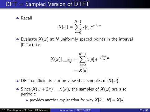
DFT = Sampled Version of DTFT

Recall

X (ω) =N−1∑n=0

x [n] e−jωn

Evaluate X (ω) at N uniformly spaced points in the interval[0, 2π), i.e.,

X (ω)|ω= 2πkN

=N−1∑n=0

x [n] e−j 2πkN

n

= X [k]

DFT coefficients can be viewed as samples of X (ω)

Since X (ω + 2π) = X (ω), the samples of X (ω) are alsoperiodic

provides another explanation for why X [k + N] = X [k]


Frequency domain sampling introducestime-domain periodicity!

Sampling in the frequency domain leads to periodic repetitionin the time domain

Repetition period is N

If we sample the DTFT at L (> N) points, the repetitionperiod will be L (> N)

If x [n] is of duration N, then X (ω) has to be sampled at leastat N points to avoid aliasing in the time domain


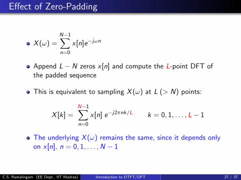
Effect of Zero-Padding

X (ω) =N−1∑n=0

x [n]e−jωn

Append L− N zeros x [n] and compute the L-point DFT ofthe padded sequence

This is equivalent to sampling X (ω) at L (> N) points:

X [k] =N−1∑n=0

x [n] e−j2πnk/L k = 0, 1, . . . , L− 1

The underlying X (ω) remains the same, since it depends onlyon x [n], n = 0, 1, . . . ,N − 1


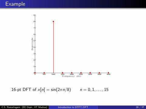
Example

0 500 1000 1500 2000 2500 3000 3500 40000

1

2

3

4

5

6

7

8

9

Frequency (Hz)

Magnitude

16-pt DFT of x [n] = sin(2πn/8) n = 0, 1, . . . , 15


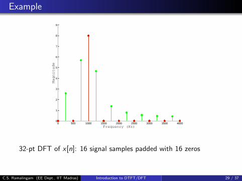
Example

0 500 1000 1500 2000 2500 3000 3500 40000

1

2

3

4

5

6

7

8

9

Frequency (Hz)

Magnitude

32-pt DFT of x [n]: 16 signal samples padded with 16 zeros


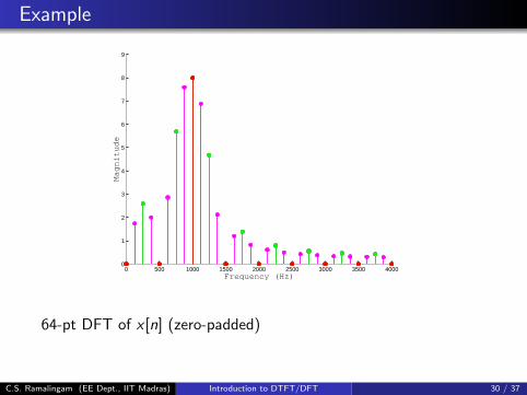
Example

0 500 1000 1500 2000 2500 3000 3500 40000

1

2

3

4

5

6

7

8

9

Frequency (Hz)

Magnitude

64-pt DFT of x [n] (zero-padded)


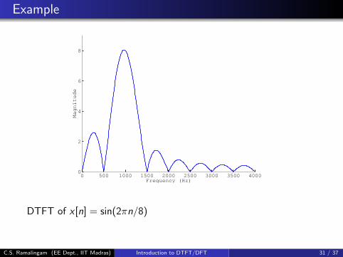
Example

0 500 1000 1500 2000 2500 3000 3500 40000

2

4

6

8

Frequency (Hz)

Magnitude

DTFT of x [n] = sin(2πn/8)


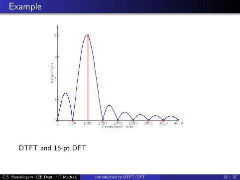
Example

0 500 1000 1500 2000 2500 3000 3500 40000

2

4

6

8

Frequency (Hz)

Magnitude

DTFT and 16-pt DFT


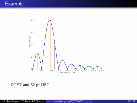
Example

0 500 1000 1500 2000 2500 3000 3500 40000

2

4

6

8

Frequency (Hz)

Magnitude

DTFT and 32-pt DFT


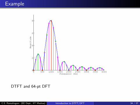
Example

0 500 1000 1500 2000 2500 3000 3500 40000

2

4

6

8

Frequency (Hz)

Magnitude

DTFT and 64-pt DFT


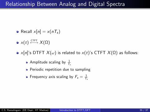
Relationship Between Analog and Digital Spectra

Recall x [n] = x(nTs)

x(t)CTFT←→ X (Ω)

x [n]’s DTFT X (ω) is related to x(t)’s CTFT X (Ω) as follows:

Amplitude scaling by 1Ts

Periodic repetition due to sampling

Frequency axis scaling by Fs = 1Ts


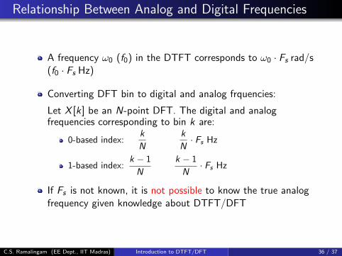
Relationship Between Analog and Digital Frequencies

A frequency ω0 (f0) in the DTFT corresponds to ω0 · Fs rad/s(f0 · Fs Hz)

Converting DFT bin to digital and analog frquencies:

Let X [k] be an N-point DFT. The digital and analogfrequencies corresponding to bin k are:

0-based index:k

N

k

N· Fs Hz

1-based index:k − 1

N

k − 1

N· Fs Hz

If Fs is not known, it is not possible to know the true analogfrequency given knowledge about DTFT/DFT


Introduction to the Discrete-Time Fourier Transform and ...

Documents

Transcript of Introduction to the Discrete-Time Fourier Transform and ...