Testing Conditional Independence using Conditional Martingale Transforms

Kyungchul Song1

Department of Economics, University of Pennsylvania

November 28, 2006

Abstract

This paper investigates the problem of testing conditional independence between Y and

Z given λ0(X) where λ0 is an unknown parametric or nonparametric real-valued func-

tion and a consistent estimator λ is available. First, the paper analyzes the asymptotic

power properties of the tests via approximate Bahadur asymptotic relative efficiency

and demonstrates that there is improvement in power when we use nonparametric es-

timators of conditional distribution functions in place of true ones. Second, the paper

proposes a method of conditional martingale transforms under which tests are asymp-

totically distribution free and asymptotically unbiased against√n-converging Pitman

local alternatives. We find that when Y and Z are continuous, the power improvement

from the nonparametric estimation disappears after the conditional martingale trans-

form, but when either of Y or Z is binary, this phenomenon of power improvement

appears even after the conditional martingale transform. We perform Monte Carlo

simulation studies to compare the martingale transform approach and the bootstrap

approach, and also compare small sample powers of tests with nonparametrically esti-

mated distribution functions and true ones.

Key words and Phrases: Conditional independence, Asymptotic pivotal tests, condi-

tional martingale transforms, approximate Bahadur ARE.

JEL Classifications: C12, C14, C52.

1 Introduction

This paper proposes a new class of tests of conditional independence between Y and Z given an

index λ0(X) of X, where λ0 is either parametrically or nonparametrically specified. Conditional

1 I am grateful to Yoon-Jae Whang and Guido Kuersteiner who gave me valuable advice at the initial stage ofthis research. I also thank Hyungsik Roger Moon, Qi Li, Joon Park, Norm Swanson and seminar participants ata KAEA meeting and a workshop at Rutgers University and Texas A&M for their valuable comments. All errorsare mine. Address correspondence to: Kyungchul Song, Department of Economics, University of Pennsylvania, 528McNeil Building, 3718 Locust Walk, Philadelphia, Pennsylvania 19104-6297.

1

independence restrictions are used in a variety of contexts of econometric modeling, and often serve

as a testable implication of identifying restrictions. See the next section for relevant examples.

The literature of testing conditional independence is recent and, apparently, involves relatively

few researches as compared to that of other nonparametric or semiparametric tests. Linton and

Gozalo (1999) proposed tests that are slightly stronger than tests of conditional independence.

Recently, Su and White (2003a, 2003b, 2003c) studied several methods of testing conditional inde-

pendence. Angrist and Kuersteiner (2004) suggested distribution-free tests of conditional indepen-

dence.

This paper’s framework of hypothesis testing is based on an unconditional-moment formulation

of the null hypothesis using indicator functions that run through an index space. Tests in our

framework have the usual local power properties that are shared by other empirical-process based

approaches such as Linton and Gozalo (1999) and Angrist and Kuersteiner (2004). In particular,

the tests are asymptotically unbiased against√n-converging Pitman local alternatives. In contrast

with Linton and Gozalo (1999), our tests are asymptotically pivotal (or asymptotically distribution-

free), which means that asymptotic critical values do not depend on unknowns, so that one does not

need to resort to a simulation-based method like bootstrap to obtain approximate critical values.

This latter property of asymptotic pivotalness is shared, in particular, by Angrist and Kuer-

steiner (2004) whose approach is close to ours in two aspects.2 First, their test has local power

properties that are similar to ours. Second, both their approach and ours employ a method of

martingale-transform to obtain asymptotically distribution free tests. However, they assume that

Z is binary and the conditional probability P{Zi = 1|Xi} is parametrically specified, whereaswe do not require such conditions. This latter contrast primarily stems from completely dif-

ferent approaches of martingale transforms employed by the two papers. In particular, Angrist

and Kuersteiner (2004) employ martingale transforms that apply to tests involving estimators

of finite-dimensional parameters, whereas this paper uses conditional martingale transforms that

are amenable to testing semiparametric restrictions that involve nonparametric estimators (Song

(2006b)).

The martingale transform approach was pioneered by Khmaladze (1988,1993) and has been used

both in the statistics and economics literature. For example, Stute, Thies, and Zhu (1998) and

Khmaladze and Koul (1994) studied testing nonlinear parametric specification of regressions. Koul

and Stute (1999) proposed specification tests of nonlinear autoregressions. Recently in the econo-

metrics literature, Koenker and Xiao (2002) and Bai (2003) employed the martingale transform

approach for testing parametric models, and Angrist and Kuersteiner (2004) investigated testing

conditional independence as mentioned before. Song (2006b) developed a method of conditional

martingale transform that applies to tests of semiparametric conditional moment restrictions. Al-

2Several tests suggested by Su and White are also asymptotically pivotal, and consistent, but have differentasymptotic power properties. Their tests are asymptotically unbiased against Pitman local alternatives that convergeto the null at a rate slower than

√n. However, when we extend the space of local alternatives beyond Pitman local

alternatives, the rate of convergence of local alternatives that is optimal is typically slower than√n.(e.g. Horowitz

and Spokoiny (2002)).

2

though the conditional independence restrictions can be viewed as a special case of semiparametric

conditional moment restrictions, the restrictions are not encompassed by the framework of Song

(2006b).

As by-product, we find that the nonparametric estimation error of F (y|u) improves the asymp-totic power of the test. Here F (y|u) denotes a nonparametric estimator of F (y|u), the conditionaldistribution function of Y given U , Fλ0(λ0(X)), where Fλ0(·) denotes the distribution function ofλ0(X). This gives rise to a counter-intuitive consequence that even when the true nonparametric

function F (y|u) is known, the estimation of the function improves the performance of the test. Weformally show this in terms of approximate Bahadur asymptotic relative efficiency. We provide

intuitive explanation for this, by identifying the restrictions that are utilized more effectively in

nonparametric estimation than when we use true ones.

When Y and Z are continuous, we apply conditional martingale transforms to the indicator

functions involving Y and Z. Since the conditional martingale transforms remove the additional

local shift caused by the nonparametric estimation error in F (y|u), the phenomenon of improvedasymptotic power by nonparametric estimation errors does not arise after we apply the conditional

martingale transforms. However, when Z is binary, this phenomenon of improved local asymptotic

power reappears, because in this case it suffices to take conditional martingale transform only on

the continuous variable Y.

It is interesting to analyze the effect of the conditional martingale transform on the asymptotic

power properties of tests. To this end, we compute the approximate Bahadur asymptotic relative

efficiency of a Kolmogorov-Smirnov type test that uses the original empirical process relative to

one that uses the transformed empirical process. From the result, we characterize a certain set of

alternatives under which the conditional martingale transform improves the asymptotic power of

the test.

We perform a small scale Monte Carlo simulations to compare the approach of bootstrap and

that of martingale transforms. Although the results are at a preliminary stage, the martingale

transform appears to perform as well as bootstrap.

In the next section, we define the null hypothesis of conditional independence and present the

asymptotic representation of the semiparametric empirical process. In Section 3, we construct con-

ditional martingale transforms and show how they can be used to generate a class of asymptotically

pivotal tests. In Section 4, we present feasible transforms using series-based methods. In Section 5,

we consider the case where Zi is binary as in Angrist and Kuersteiner (2004) and discuss how this

case can be accommodated into our framework. The implementation of the transform approach

becomes even simpler in this case. In Section 5, we discuss results from simulation studies that

compare the bootstrap approach and the martingale transform approach. In Section 6, we conclude.

3

2 Testing Conditional Independence

2.1 The Null and Alternative Hypotheses

Suppose that we are given with a random vector (Y,Z,X) distributed by P and an unknown real

valued function λ0(·) on RdX that satisfy the following conditions:

Assumption 1 : (i) Y and Z are continuous random variables with support in [0, 1]

(ii) λ0(X) is a continuous random variable with a distribution function F0.

When either Y or Z is binary, the development of this paper’s thesis becomes simpler. We will

discuss the case when Z is binary in a later section. The thesis of this paper can be extended to the

case of Y and Z being random vectors, only to cause more complicated notations. Our restricting

the support of (Y,Z) into a unit square is innocuous, since we can transform its marginals using

a strictly increasing function taking values in [0, 1]. Condition (ii) is mostly satisfied, unless the

function λ0(·) is equal to a constant over an area in which X has a positive support. Condition (ii)

is convenient, enabling us to employ a quantile transform of the conditioning variable λ0(X). The

quantile transform is useful because as it turns out later, the estimation error from the estimator

λ of λ0 does not alter the asymptotic representation of the test statistic.

We are interested in testing the null hypothesis of conditional independence of Y and Z given

λ0(X). Since the distribution function F0 of λ0(X) is strictly increasing on the support of λ0(X),

the σ-field generated by λ0(X) is equal to that generated by its quantile transform U = F0(λ0(X)).

By using notations for indicator functions:

γz(Z) , 1{Z ≤ z}, γy(Y ) , 1{Y ≤ y}, and γu(U) , 1{U ≤ u},

we can write the null hypothesis of conditional independence as (e.g. see Theorem 9.2.1. in Chung

(2001), p.322):

H0 : E(γy(Y )|U,Z) = E(γy(Y )|U), P-a.s. ∀y ∈ [0, 1]. (1)

Then the alternative hypothesis is given by the negation of the null:

H1 : P{E(γy(Y )|U,Z) = E(γy(Y )|U) for some y ∈ [0, 1]} > 0.

We assume throughout the paper that to each potential data generating process P corresponds

a unique function λ0(·). This means that a unique function λ0(·) is identified from the data gen-

erating process P regardless of whether it belongs to the null hypothesis or to the alternatives.

In the next subsection, we discuss two examples of econometric specifications that use conditional

independence.

4

2.2 Examples

2.2.1 Nonseparable Models

Conditional independence restriction is often used in nonseparable models. The first example is a

model of weakly separable endogenous dummy variables. Suppose Y and Z are generated by

Y = g(ν1(X,Z), ε) and

Z = 1 {ν2(X) ≥ u} .

For example, this model can be useful when a researcher attempts to analyze the effect of job

training of a worker upon her earnings prospects. Here Y denotes the earnings outcome of a worker,

and Z denotes the indicator for the job training. It will be of interest to a researcher whether

the indicator for the job training remains still endogenous even after controlling for covariates

X, because in the presence of endogeneity, the researcher might need to include some additional

covariate into the specification of the endogenous job training that has a sufficient degree of variation

independent fromX. (e.g. Vytlacil and Yildiz (2006)). The exogeneity of Z for the outcome Y given

the covariate X will be represented by the conditional independence restriction:

Y ⊥ Z|ν1(X,Z), ν2(X).

A second example is from Altonji and Matzkin (2005) who considered the following nonseparable

regression model.

Y = m(Z, ε).

One of the assumption used to identify the local average response was that ε is independent of

Z given an instrumental variable X. This gives the following testable implication of conditional

independence restriction (e.g. Dawid (1980)),

Y ⊥ Z|X.

2.2.2 Heterogeneous Treatment Effects

In the literature of heterogeneous treatment effects, often the restriction of conditional independence

(Y0, Y1) ⊥ Z | X

is considered.(e.g. Rubin (1978), Rosenbaum and Rubin (1983), and Hirano, Imbens, and Ridder

(2003) to name but a few.)3 This conditions is also called the condition of unconfounded treatment

assignment. Here Y0 represents the outcome when an agent is not treated and Y1, the outcome when

treated. The conditional probability of being treated p(X) = P (Z = 1|X) given the covariate X3 It is also worth noting that Heckman, Ichimura, and Todd (1998) point out that a weaker condition of mean

independence suffices for the identication of the average treatment effect.

5

is called the propensity score. When p(X) ∈ (0, 1), it follows that (Rosenbaum and Rubin (1983))

(Y0, Y1) ⊥ Z | p(X).

This restriction is not directly testable because we do not observe Y0 and Y1 simultaneously for

each individual. We can at least test its implications:

(1− Z)Y ⊥ Z | p(X) or ZY ⊥ Z | p(X).

While we may specify p(·) parametrically, the procedure of this paper also allows for the case whenp(·) is specified as a nonparametric function.

3 An Asymptotic Representation of a Semiparametric EmpiricalProcess

3.1 Asymptotic Representation

The null hypothesis of (1) is a conditional moment restriction. We can obtain an equivalent for-

mulation in terms of unconditional moment restrictions. Let us define

gy(u) , E(γy(Y )|U = u) and gz(u) , E(γz(Y )|U = u)

Then the null hypothesis can be written as:

H0 : E[γu(U)γz(Z)(γy(Y )− gy(U))] = 0, ∀(y, z, u) ∈ [0, 1]3.

Test statistics we analyze in the paper are based on the sample analogue of the above mo-

ment restrictions. Suppose that we are given a random sample {Si}ni=1 = {(Yi, Zi, Ui)}ni=1 ofS = (Y,Z,U). If the function gy(·) were known and the quantile transformed data Ui were ob-

served, a test statistic could be constructed as a functional of the following stochastic process:

νn(r) ,1√n

nXi=1

γu(Ui)γz(Zi)(γy(Yi)− gy(Ui)), r = (y, z, u). (2)

The process cannot be used to construct a test statistic because it involves unknown gy. In this

section, we introduce a series estimator of gy and investigate the asymptotic properties of the

resulting empirical process that involves the estimator.

We approximate gy(u) by pK(u)0πy which is constituted by a basis function vector pK(u) anda coefficient vector πy. Given an appropriate estimator λ(·) of λ(·), define

Ui ,1

n

nXj=1,j 6=i

1nλ(Xj) ≤ λ(Xi)

o. (3)

6

The series-based estimator is defined as gy(u) , pK(u)0πy, where πy , [P 0P ]−1P 0ay,n with ay,n andP being defined by

ay,n ,

⎡⎢⎢⎣γy(Y1)...

γy(Yn)

⎤⎥⎥⎦ and P ,

⎡⎢⎢⎣pK(U1)

0...

pK(Un)0

⎤⎥⎥⎦ .Using the estimated conditional mean function gy, we can construct a feasible version of the process

νn(r) :

νn(r) =1√n

nXi=1

γu(Ui)γz(Zi)(γy(Yi)− gy(Ui)).

We call the process νn(r) a semiparametric empirical process. A test statistic can be constructed

as a known functional of the process νn(r). Our main result in this section provides a uniform

asymptotic representation of the process νn(r) that holds both under the null hypothesis and

under the alternatives. To this end, we introduce notations and assumptions.

We define the Lp(P) norm k·kp by ||g||p , (E kg(Si)kp)1/p and define a uniform norm || · ||∞ by

||g||∞ , sups |g(s)|. We also introduce the notation

ζν,K , supµ≤ν

supu|DµpK(u)|, (4)

where Dµ is the derivative operator defined by

Dµg(u) , (∂|µ|/∂zµ11 · · · ∂zµdZdZ)(g(u)). (5)

The notation à denotes weak-convergence in the sense of Hoffman-Jorgensen (e.g. van der Vaart

and Wellner (1996)). Let FZ|U (z|u) and fZ|U(z|u) denote the conditional distribution function andthe conditional density of Zi given Ui.We define similarly FY |U (y|u) and fY |U (y|u). Let N[](ε,Λ, || ·||p) denote the Lp-bracketing number, i.e., the smallest number r of pairs of functions (λj ,∆j)

rj=1

in Lp(P) such that ||∆j ||p < ε, and for all λ ∈ Λ, there exists a pair (λj ,∆j), j ∈ {1, ··, r} satisfyingthe inequality: |λj(x)− λ(x)| < ∆j(x).

Assumption 2 : (i) (Yi, Zi,Xi)ni=1 is a random sample from P where E||Y ||p <∞, E||Z||p <∞

and E||X||p <∞ for some p > 4. (ii) There exist a class Λ of functions that contain λ0 and satisfy

that:(a) for a constant b1 ∈ [0, 2), logN[](ε,Λ, || · ||∞) < Cε−b1 , (b) ||λ − λ0||∞ = oP (n−1/4), and

(c) P{λ ∈ Λ}→ 1 as n→∞, where F is the distribution function of X.

When Λ is a parametric class such that Λ ,©λθ : θ ∈ Θ ⊂ Rdθ

ªwith Θ being compact and λθ

is locally uniformly Lp-continuous in θ ∈ Θ in the sense of Chen, Linton, and van Keilegom (2003),

the condition (ii)(a) holds for arbitrarily small b > 0. The condition of Lp-uniform continuity is

much weaker than the requirement that λθ be Lipschitz in θ. When λ0 is a nonparametric function,

we can take Λ to be a function space containing λ0. The uniform consistency of λ for λ0 is required

to hold both under the null hypothesis and under the alternatives. We may view λ0 as a uniform

7

probability limit of λ. Condition (ii)(c) can be fulfilled, for instance, by taking a smooth basis

functions.

Let us define a shrinking neighborhood of λ0 : Λn , {λ ∈ Λ : ||λ − λ0||∞ ≤ Cn−b}, forb ∈ (1/4, 1/2] and for some positive constant C > 0. The following are a set of assumptions for

basis functions.

Assumption 3 : (i) λmin¡R

pK(u)pK(u)du¢> 0.

(ii) There exist d1 and d2 such that (a) for some d > 0, there exist sets of vectors {πy : y ∈ [0, 1]}and {πz : z ∈ [0, 1]} such that

sup(y,u)∈[0,1]2

¯pK(u)0πy − gy(u)

¯= O(K−d1) and

sup(z,u)∈[0,1]2

¯pK(u)0πz − gz(u)

¯= O(K−d2),

(b) for each u ∈ [0, 1] there exist sets of vectors in RK , {πy,u : y ∈ [0, 1]}, such that

sup(y,u)∈[0,1]×[0,1]

µZ 1

0

¯PK(u)0πy,u − gy(u)1{u ≤ u}¯p du¶1/p = O(K−d1).

(iii) For d1 and d2 in (ii),√nζ20,KK

−d = o(1) and√nζ1,KK

−d2 = o(1)

(iv) For b in the definition of Λn, we have n1/2−2bζ30,Kζ2,K = o(1), n−1/2+1/pK1−1/pζ20,K = o(1) and

n−bζ0,K{pζ0,Kζ2,K + ζ1,K} = o(1).

Condition (i) is used by Andrews (1991) and Newey (1997), and can be satisfied by choosing an

orthonormal basis function that is supported in [0, 1]. Condition (ii) requires the rate of convergence

for uniform approximation errors to be of a polynomial order in K.

Assumption 4 : (i) The density fλ(λ) of λ(X) satisfies supλ∈Λn supλ∈R fλ(λ) <∞.

(ii) For some C > 0, supλ∈Λnsupλ∈Sλ¯Fλ(λ+ δ)− Fλ(λ− δ)

¯< Cδ, for all δ > 0.

(iii) There exists C > 0 such that for each u, u1 ∈ U , {Fλ ◦ λ : λ ∈ Λn} and for each u2 ∈ [0, 1],

sup(u1,u)∈[0,1]2:|u2−u1|<δ

|P (Y ≤ y, u1(X) ≤ u|u(X) = u1)− P (Y ≤ y, u1(X) ≤ u|u(X) = u2)|

≤ ϕu,u1(y, x)δ,

where ϕu,u1(·, ·) is a real function that satisfies supx∈SXR |α(y)|ϕu,u1(y, x)dy < C and

Rϕu,u1(y, x)dx <

CfY (y) with fY (·) denoting the density of Y.(iv) The conditional distribution functions FY |U (y|u) and FZ|U (z|u) are second-order continuouslydifferentiable with uniformly bounded derivatives.

Conditions in Assumption 4 are concerned about the densities and conditional densities of Y, Z,

and λ(X). The conditions are primarily used to resort to a lemma in Escanciano and Song (2006)

8

on which the result of Theorem 1 below relies. Condition (i) requires that the density of λ(X) for

λ ∈ Λn is uniformly bounded. A similar condition was used by Stute and Zhu (2005). Condition (ii)says that the distribution function of λ(X) should be Lipschitz continuous with Lipschitz coefficient

uniformly bounded over Λn. Condition (iii) requires Lipschitz continuity of conditional distribution

of (Y, u1(X)), u ∈ U , given u(X) in the conditioning variable.

Theorem 1 : Suppose Assumptions 1-4 hold. Then the following holds:

supr∈[0,1]3

¯¯νn(r)− 1√

n

nXi=1

γu(Ui) {γz(Zi)− gz(Ui)}©γy(Zi)− gy(Ui)

ª¯¯ = oP (1). (6)

The result of Theorem 1 provides a uniform asymptotic representation of the semiparametric

empirical process νn(r). This asymptotic representation motivates the construction of proper condi-

tional martingale transforms that we develop in a later section. The representation also constitutes

the basis upon which we derive the power properties of the test. Indeed, observe that the process

1√n

nXi=1

γu(Ui) {γz(Zi)− gz(Ui)}©γy(Zi)− gy(Ui)

ªis a zero mean process only when the null hypothesis of conditional independence is true. From the

asymptotic representation, we can derive the asymptotic properties of the process νn(r) as follows.

Corollary 1 : (i) (a) Under the null hypothesis, νn(r) Ã ν(r), where ν is a Gaussian process

whose covariance kernel is given by

c(r1; r2) =

Z u1∧u2

−∞C(w1, w2;u)du

with C(w1, w2;u) = FZ|U (z1 ∧ z2|u)× {FY |U (y1 ∧ y2|u)− FY |U (y1|u)FY |U (y2|u)}.(b) Under fixed alternatives, n−1/2νn(r)Ã hγu, γz(γy − gy)i.(ii) (a) Under the null hypothesis, νn(r)Ã ν1(r), where ν1 is a Gaussian process whose covariance

kernel is given by

c1(r1; r2) =

Z u1∧u2

−∞C1(w1, w2;u)dF (u)

with

C1(w1, w2;u) =£FZ|U (z1 ∧ z2|u)− FZ|U(z1|u)FZ|U (z2|u)

¤×£FY |U (y1 ∧ y2|u)− FY |U (y1|u)FY |U (y2|u)¤.

(b) Under fixed alternatives, n−1/2νn(r)Ã hγu, γz(γy − gy)i.

The results of Corollary 1 lead to the asymptotic properties of tests based on the processes νn(r)

and νn(r). The limiting processes ν(r) and ν1(r) under the null hypothesis are Gaussian processes

with different covariance kernels. Under the fixed alternatives, the two empirical processes νn(r)

9

and νn(r) weakly converge to the same shift term after the normalization by√n. This has two

interesting consequences. First, the local power properties under√n-converging Pitman local

alternatives naturally follow from this result. Second, the result in Corollary 1 gives rise to a

surprising consequence that using the nonparametrically estimated distribution function F (y|u)instead of the true one F (y|u) can improve the asymptotic power of the tests. In particular, thecovariance kernel of the limit process under the null hypothesis "shrinks" due to the use of F (y|u)instead of F (y|u) whereas the limit shift hγu, γz(γy − gy)i under the alternatives remains intact.In a subsequent subsection, we formalize this observation using approximate Bahadur asymptotic

relative efficiency.

It is worth noting that the estimation error in λ does not play a role in determining the limit

behavior of the process νn(r). In other words, the results of Theorem 1 and Corollary 1 do not

change when we replace λ by λ0. A similar phenomenon is discovered and analyzed in Stute and

Zhu (2005) in the context of testing single-index restrictions using a kernel method. This convenient

phenomenon is due to the use of the empirical quantile transform of λ(Xi).

We construct the following test statistics:

TKS = supr∈[0,1]3

|νn(r)| and TCM =

Z[0,1]3

νn(r)2dr. (7)

The test statistic TKS is of Kolmogorov-Smirnov type and the test statistic TCM is of Cramér-von

Mises type. The asymptotic properties of the tests based on TKS and TCM follow from Theorem

1. Indeed, under the null hypothesis,

TKS Ã supr∈[0,1]3

|ν(r)| and TCM ÃZ[0,1]3

ν1(r)2dr,

and under the Pitman local alternativesPn such that for some ay,z(·), En(γz(Z)(γy(Y )−gy(U))|U =u) = ay,z(u)/

√n+ o(n−1/2),

νn(r)Ã ν1(r) + hγu, ay,zi.

The presence of the non-zero shift term hγu, ay,zi renders the test to have nontrivial asymptoticpower against such local alternatives.

The asymptotic critical values cannot be computed directly from the limiting distributions of the

test statistics, because the test statistics depend on unknown components of the data generating

process and in consequence the tests are not asymptotically pivotal. This stems from the fact

that the limiting Gaussian processes ν(r) and ν1(r) have complicated kernels which, in particular,

contain Brownian bridge type components

FY |U (y1 ∧ y2|u)− FY |U (y1|u)FY |U (y2|u) andFZ|U (z1 ∧ z2|u)− FZ|U (z1|u)FZ|U (z2|u).

This source of complication is different in nature from the one that is simply due to the estimation

10

error of parameters in the conditional moment restriction (e.g. Stute (1997), Stute, Thies and

Zhu (1998), Khmaladze and Koul (2005), Song (2006b)). Rather, the situation is close to the

fundamental problem of goodness-of-fit tests of multivariate distributions (e.g. Khmaladze (1993))

in which the limiting distribution of a test statistic is equal to a functional of a multiparameter

Brownian bridge.

There are primarily two approaches to deal with this problem: the bootstrap approach and the

martingale transform approach. The bootstrap approach uses critical values from the distribution

of bootstrap samples. The martingale transform approach transforms the test so that critical values

can be tabulated from the first order asymptotic theory. This paper focuses on developing the latter

approach.

3.2 The Effect of Nonparametric Estimation Error

We analyze how our use of a nonparametric estimator for F (y|u) in the process νn(r) affects thepower of the test. Surprisingly, we find that the power of the test improves by using the estimator

instead of a true one. In other words, the test becomes better when we use estimator F (y|u) even ifwe know the true conditional distribution function F (y|u). This is because the use of nonparametricestimator has an effect of "shrinking" the covariance of the limiting process ν(r) under the null

hypothesis while preserves the local shift under the Pitman local alternatives.

We formalize this observation by employing the notion of approximate Bahadur asymptotic

relative efficiency (ARE). Approximate Bahadur ARE was introduced by Bahadur (1960) and has

been widely used in the literature (see Nikitin (1995) and references therein). While it is more

desirable to use exact Bahadur efficiency, approximate Bahadur efficiency is very easy to compute

and can provide a quick idea in comparison of tests (Nikitin (1995)). We relegate a further analysis

using exact Bahadur efficiency to a future research.

Suppose Γ is a known continuous functional that is homogeneous of degree one, is applied

to stochastic processes νn(r) and νn(r) and used to construct a test statistic. For example, the

Cramér-von Mises type test statistics can be defined as Γνn and Γνn with Γ being a functional

defined by Γg =Rg2(r)dr. Then denote by H0(v) and H1(v) the limits of the rejection probability

of tests based on Γνn and Γνn under the null hypothesis. That is, under the null hypothesis,

P {Γνn ≥ v}→ h0(κ) and P {Γνn ≥ κ}→ h1(κ)

as n→∞. This often boils down to the computation of tail probabilities of a functional of Gaussian

processes. Suppose the functional Γ is taken to be homogeneous of degree one and there exist

constants b0 and b1 satisfying

lnh0(κ) = −12b0κ

2 + o(1) and lnh1(κ) = −12b1κ

2 + o(1) as κ→∞.

On the other hand, under the fixed alternative P1, suppose we have functions ϕ0 and ϕ1 on

11

[0, 1]3 such that

1√nΓνn = Γ

µ1√nνn

¶→p Γϕ0, and (8)

1√nΓνn = Γ

µ1√nνn

¶→p Γϕ1.

Then the approximate Bahadur ARE (denoted by e0,1(P1)) of a test based on the test statistic Γνnrelative to one that is based on Γνn is computed from (Nikitin (1995)),

qe0,1(P1) =

rb0b1× Γϕ0Γϕ1

.

The approximate Bahadur ARE is composed of two ratios. The first ratio b1/b0 measures the

relative tail behavior of the limiting distribution of the test statistic under the null hypothesis. The

second ratio Γϕ0/Γϕ1 measures how sensitively the test statistics deviate from the null limiting

distribution in large samples under the alternatives. When e0,1(P1) < 1, it is likely that the power

of the test based on Γνn is better than one based on Γνn. The following result shows that this is

indeed the case.

Corollary 2 : Suppose the conditions of Theorem 1 hold and choose the Kolmogorov-Smirnov

functional Γν(r) = supr∈[0,1]3 |ν(r)|. Then

e1,0(P1) =1

4.

The result in Corollary 2 is well expected from the result of Theorem 1. The main reason is

because using the nonparametric estimator F (y|u) in place of F (y|u) has an effect of "shrinking"the kernel of the limiting Gaussian process from

c0(r1, r2) = (u1 ∧ u2)(z1 ∧ z2)(y1 ∧ y2 − y1y2)

to c1(r1, r2) = (u1 ∧ u2)(z1 ∧ z2 − z1z2)(y1 ∧ y2 − y1y2). Hence with the same fixed level α, the

critical value based on the second Gaussian process is smaller than the first Gaussian process. On

the other hand the local limit shifts of the test statistics under the alternatives are identical to

hγu, ρwi regardless of whether one uses F (y|u) or F (y|u). This yields the counter-intuitive resultthat even when we know the conditional distribution function F (y|u), it is better to use its estimatorF (y|u) in the test statistic.4

4Khmaladze and Koul (2005) also discuss the case when the power is increased by using estimators instead of trueones in the context of parametric tests.

12

3.3 Discussion

In the literature of estimation, there are findings that report that under certain circumstances, the

estimation of nonparametric functions improves the efficiency of the estimators upon that when true

functions are used. (e.g. Hahn (1998), and Hirano, Imbens, and Ridder (2003) and see references

therein.) This efficiency gain arises due to the fact that the nonparametric estimation utilizes the

additional restrictions in a manner that is not utilized when we use the true ones. We give an

explanation of our findings in the preceding section in a similar vein.

The primary source of the improvement of the asymptotic power stems from the following

asymptotic representation (for a general result, see Lemma 1U of Escanciano and Song (2006))

1√n

nXi=1

γu(Ui)γz(Zi){γy(Yi)− gy(Ui)}

=1√n

nXi=1

γu(Ui){γz(Yi)− gz(Ui)}{γy(Yi)− gy(Ui)}+ oP (1).

As noted in the remarks after Theorem 1, the variance of the leading sum on the right-hand side is

smaller than that of 1√n

Pni=1 γu(Ui)gz(Zi){γy(Yi) − gy(Ui)} under the null hypothesis. When we

replace γz(Z) by gz(U) on the left-hand side, we obtain the following result

1

n

nXi=1

γu(Ui)gz(Ui){γy(Yi)− gy(Ui)} = oP (n−1/2). (9)

This fact provides a contrast to the result obtained using the true nonparametric function gy :

1

n

nXi=1

γu(Ui)gz(Ui){γy(Yi)− gy(Ui)} = OP (n−1/2). (10)

The rate of convergence for the sample version of E£γu(U)gz(U){γy(Y )− gy(U)}

¤is faster with

the nonparametric estimator gy than the true one. Actually we can obtain the same contrast be-

tween (9) and (10) when we replace γu(U)gz(U) by any function ϕ(U). In other words, by using

the nonparametric estimation in the test statistic, we utilize the conditional moment restriction

E£γy(Y )− gy(U)|U

¤= 0 more effectively than by using the true function gy. The conditional

moment restriction holds both under the null hypothesis and under the alternatives. Under the

alternatives, this effective utilization of the conditional moment restriction by nonparametric esti-

mation has an effect of order that is dominated by the√n-diverging shift term which remains the

same regardless of whether we use gy or gy. Combined with this, the first order effect of nonpara-

metric estimation under the null hypothesis results in improvement in power over the test using

the true one gy.

13

4 Conditional Martingale Transform

A recent work by the author (Song (2006b)) demonstrates that the method of conditional martingale

transform can be useful to obtain asymptotically pivotal semiparametric tests. The method of

conditional martingale transform proposed in the work does not apply to the testing problem of

conditional independence for two reasons. First, the generalized residual function ρy,z , γz(γy −gy) is indexed by (y, z) ∈ [0, 1]2 whereas the generalized residual function ρτ,θ in Song (2006b)

does not depend on the index of the empirical process. Second, while Song (2006b) requires

that the conditional distribution of instrumental variables conditional on the variable inside the

nonparametric function should not be degenerate, this condition does not hold here. In the current

situation of testing conditional independence, the instrumental variable in the conditional moment

restriction and the variable inside the nonparametric function are identically X. Therefore, the

nondegeneracy of the conditional distribution fails.

The main idea of this paper is that first, we take into account the null restriction of conditional

independence when we search for a proper transformation of the semiparametric empirical process

νn(r) using conditional martingale transforms, and then analyze the asymptotic behavior of the

semiparametric empirical process after the transform.5

4.1 Preliminary Heuristics

In this section, we provide some heuristics of the mechanics by which conditional martingale trans-

forms work. Let us define the conditional inner product h·, ·iu by

hf, giu ,Z(fg)(s)dF (s|u)

where F (s|u) is the conditional distribution function of S given U = u. Suppose that we are

given with an operator K on the space of indicator functions such that the transformed indicator

functions γKz , Kγz and γKy , Kγy satisfy the orthogonality condition and the isometry conditionwith respect to the conditional inner product almost surely:

Conditional Orthogonality : hγKz , 1iU = 0 and hγKy , 1iU = 0, andConditional Isometry : hγKz1 , γKz2iU = hγz1 , γz2iU and hγKy1 , γKy2iU = hγy1 , γy2iU .

An operator K that satisfies these two properties can be used to construct a transformed empiricalprocess from which asymptotically distribution free tests can be generated. Recall that by Theorem

1, the process νn(r) has the following asymptotic representation (using our conditional inner product

5By noting that the limiting processes ν and ν1 are variants of a 4-sided tied down Kiefer process, we may considera martingale transform for a 4-sided tied down Kiefer process that was suggested by McKeague and Sun (1996). Themartingale transform for this case is represented as two sequential martingale transforms. However, the sequentialmartingale transforms will be very complicated in practice because it involves taking repreated martingale transformsof a function.

14

notation: hγy, 1iUi , E£γy(Yi)|Ui

¤)

νn(r) =1√n

nXi=1

γu(Ui) {γz(Yi)− hγz, 1iUi}©γy(Yi)− hγy, 1iUi

ª+ oP (1).

When we replace the indicator functions γz and γy by the transformed ones γKz and γKy , the right-

hand side asymptotic representation turns into the following (by the conditional orthogonality of

the transform):

1√n

nXi=1

γu(Ui)©γKz (Yi)− hγKz , 1iUi

ª©γKy (Yi)− hγKy , 1iUi

ª=

1√n

nXi=1

γu(Ui)γKz (Zi)γ

Ky (Yi). (11)

We can show that the last term is equal to

√nE

£γu(U)hγKz , γKy iU

¤+ νK(r) + oP (1) (12)

where νK(r) is a certain Gaussian process. The asymptotic behavior of the leading two termsdetermine the asymptotic properties of tests that are based on the transformed empirical process.

Suppose that we are under the null hypothesis. Then the first term in (12) becomes zero by the

conditional independence restriction. As shown in the appendix, the Gaussian process νK(r) has acovariance function of the form

c(r1, r2) , E[γu1∧u2(U)γz1∧z2(Z)γy1∧y2(Y )]. (13)

This form is obtained by using the conditional isometry of the operator K and the null hypothesisof conditional independence. Hence the resulting Gaussian process is a time-transformed Brownian

sheet and we can rescale it into a standard Brownian sheet by using an appropriate normaliza-

tion. Against alternatives P1 such that P1{|hγKz , γKy iU | > 0} > 0, a test properly based on the

transformed process will be consistent.

The interesting phenomenon that the nonparametric estimation error improves the power dis-

appears for tests based on transformed processes of the kind in (11). Consider the asymptotic

representation of the empirical process νn(r) that uses the true conditional distribution function

Fy(y|u) :νn(r) =

1√n

nXi=1

γu(Ui)γz(Yi)©γy(Yi)− hγy, 1iUi

ª+ oP (1).

When we apply the transform K to the indicator functions of γy and γz, the right-hand side is

15

equal to

1√n

nXi=1

γu(Ui)γKz (Yi)

©γKy (Yi)− hγKy , 1iUi

ª+ oP (1)

=1√n

nXi=1

γu(Ui)γKz (Yi)γ

Ky (Yi) + oP (1).

Hence the asymptotic representation of the process after the transform K coincides with that in

(11). The asymptotic power properties remain the same regardless of whether we use Fy(y|u) orFy(y|u) once the transform K is applied.

4.2 Conditional Martingale Transforms

In this section, we discuss a method to obtain the operator K that satisfies the conditional or-

thogonality and the conditional isometry properties. Khmaladze (1993) proposes using a class

of isometric projection operators on L2-space. This class of isometric projection operators are

designed to be an isometry in the usual inner-product in L2-space. Song (2006b) extends this iso-

metric projection to conditional isometric projection by using conditional inner-product in place of

the usual inner-product and finds that this class of projection operators can be useful to generate

semiparametric tests that are asymptotically distribution free. Just as the isometric projection is

called a martingale transform, Song (2006b) calls the conditional isometric projection a conditional

martingale transform. See Song (2006b) for the details.

By applying the conditional martingale transform in Song (2006b) to our indicator functions,

we can obtain the transform K as follows:

γKy (U, Y ) , γy(Y )−E£γy(Y )hy(U, Y )|U = u

¤y=Y

and (14)

γKz (U,Z) , γz(Z)−E [γz(Z)hz(U,Z)|U = u]z=Z ,

where

hy(U, Y ) =1{Y ≤ y}

1− FY |U (Y |U)and hz(U,Z) =

1{Z ≤ z}1− FZ|U (Z|U)

. (15)

Observe that if hy(U, Y ) and hz(U,Z) were taken to be a constant 1, the operator K is just an

orthogonal projection onto the orthogonal complement of a constant function in L2(P). The factors

hy(U, Y ) and hz(U,Z) as defined in (15) render the transforms isometric.

As compared to the conditional martingale transform in Song (2006b), the transform in this

paper corresponds to the case of function q0 in Song (2006b) being equal to 1 and hence is simpler

than typical conditional martingale transforms used to test semiparametric restrictions. This is

primarily because the estimation error of λ is no longer needed to be taken care of in the transform,

as it does not play a role in determining the asymptotic representation in Theorem 1 due to the

sample quantile transform of the conditioning variable. In order to substantiate the properties of

the conditional martingale transforms defined in (14), we introduce the following assumptions.

16

Assumption 5 : The distribution functions FY |U (·) and FZ|U (·) of Y and of Z satisfy the following:(a) for some constants C > 0, and η > 0,

supu∈[0,1]

|FY |U (y1|u)− FY |U (y2|u)| ≤ C|y1 − y2|η and

supu∈[0,1]

|FZ|U (z1|u)− FZ|U (z2|u)| ≤ C|z1 − z2|η.

(b) For any η > 0, there exists 0 < c0 < η such that for some ε > 0,

inf(y,u)∈([0,1]∩BY,0)×[0,1]

|1− FY |U (y|u)| > ε and

inf(z,u)∈([0,1]∩BZ,0)×[0,1]

|1− FZ|U (z|u)| > ε,

where BY,0 = {y : y < 1− c0} and BZ,0 = {z : z < 1− c0}.

Condition (i) is used to deal with the indicator functions 1{Y ≤ y} and 1{Z ≤ z} in thedefinition of conditional martingale transforms. The conditional martingale transform involves the

inverse of 1− FY |U (Z|U) and 1− FZ|U (Z|U). We restrict the index space for y and z to be the set

[0, 1]∩BY,0 and [0, 1]∩BZ,0 respectively. For notational brevity, we define S0 to be the corresponding

restricted index space for r :

S0 , [0, 1]× ([0, 1] ∩BY,0)× ([0, 1] ∩BZ,0).

The following result shows that the transform K defined in (14) is a martingale transform that we

have sought for. This result leads to the asymptotic properties of the process νKn (r) defined by

νKn (r) =1√n

nXi=1

γu(Ui)γKz (Zi)(γy(Yi)− gKy (Ui)),

where gKy (u) denotes the nonparametric estimator gy(u) that uses γKy in place of γy.

Theorem 2 : (i) For all y, y1 and y2 in [0, 1],

hγKy , 1iU = 0 and hγKy1 , γKy2iU = hγy1 , γy2iU almost everywhere andhγKz , 1iU = 0 and hγKz1 , γKz2iU = hγz1 , γz2iU almost everywhere.

(ii) Suppose Assumptions 1-5 hold.

(a) Under the null hypothesis,

νKn (r)Ã νK(r), (16)

where νK is a Gaussian process whose covariance kernel is given by

c3(r1; r2) ,Z u1∧u2

−∞C3(w1, w2;u)dF (u),

17

and the function C3(w1, w2;u) is defined by C3(w1, w2;u) , FZ|U (z1 ∧ z2|u)× FY |U (y1 ∧ y2|u).(b) Under the fixed alternatives,

n−1/2νKn (r)Ã E[γu(U)hγKz , γKy iU ],

where γKz and γKy are defined in (14).

The first statement of the theorem is immediately adapted from Theorem 6.1 of Khmaladze and

Koul (2004) to the "conditional inner product". This result tells us that the transform satisfies

the orthogonality condition and the isometry condition. From the results of (i) and (ii), we can

derive the asymptotic properties of tests that are constructed based on the transformed process

νKn (r). The limiting Gaussian process νK(r) is a time-transformed Brownian sheet whose kernelstill depends on the unknown nonparametric functions FZ|U and FY |U . Following a similar idea inKhmaladze (1993), we can turn the process into a standard Brownian sheet by replacing γKz (u, z)and γKy (u, y) by

γKz (u, z) ,γKz (u, z)qfZ|U (z|u)

and γKy (u, y) ,γKy (u, y)qfY |U (y|u)

,

where fZ|U and fY |U denote conditional density functions. Then the weak limit νK(r) in (16) hasa covariance function

c(r1, r2) , (u1 ∧ u2) (z1 ∧ z2) (y1 ∧ y2), r1, r2 ∈ S0,

which is that of a standard Brownian sheet.

Our test statistics are constructed based on the transformed empirical process vKn (r) defined by

νKn (r) ≡1√n

nXi=1

γu(Ui)γKz (Ui, Zi){γKy (Ui, Yi)− (PU γKy )(Ui, Yi)}.

For instance, we can construct the transformed test statistics in the following way:

TKKS = supr∈S0

¯νKn (r)

¯and TKCM =

ZS0

νKn (r)2dr. (17)

From Theorem 2, we obtain the following null limiting distribution of the test statistics:

TKKS →d supr∈S0

|W (r)| and TKCM →d

ZS0

||W (r)||2dr,

where W is a standard Brownian sheet on S0. The resulting tests based on the statistics are

asymptotically distribution free.

18

4.3 The Effect of Conditional Martingale Transforms on Asymptotic Power ofTests

Based on the result of Theorem 2, we can perform an analysis on the effect of conditional martingale

transforms on the asymptotic power using approximate Bahadur ARE. In this subsection, we

compare two tests based on the processes ν1n(r) and νKn (r). At first glance, the comparison isnot unambiguous because the martingale transform dilates the variance of the empirical process

under the null hypothesis, but at the same time moves the shift term under the local alternatives

farther from zero. The eventual comparison should take the trade-off between these two changes

into account. To facilitate the analysis, we confine ourselves to those alternatives that make such

comparison straightforward. More specifically, we consider the following specification of Y :

Y = ξ(Z, ε),

where ξ(z, ε) : [0, 1]2 → [0, 1] and ε is a random variable taking values in [0, 1] and is conditionally

independent of Z given U. In the following we give an approximate Bahadur ARE of Kolmogorov-

Smirnov tests based on the processes ν1n(r) and νKn (r) and characterize a set of alternatives underwhich the conditional martingale transform improves the asymptotic power of the test.

Let us denote the conditional copula of Z and Y given U by

CZ,Y |U (z, y|U) , P©FZ|U(Z|U) ≤ z, FY |U(Z|U) ≤ y|Uª .

The conditional copula CZ,Y |U (z, y|U) is the conditional joint distribution function of Z and Y afternormalized by the conditional quantile transforms. It summarizes the conditional joint dependence

of Z and Y given U . For introductory details about copulas, see Nelsen (1999) and for conditional

copulas, see Patton (2006).

Corollary 3 : (i) Suppose the conditions of Theorems 1 and 2 hold. Furthermore assume thatξ(z, ε) is either strictly increasing in z for all ε in the support of ε or strictly decreasing in z for

all ε in the support of ε. Then we have

e1,K(P1) = 4 supz,y

¯E£CZ,Y |U (FZ|U (z|U), FY |U (y|U)|U)− FZ|U(z|U)FY |U (y|U)

¤¯where e1,K represents the approximate Bahadur efficiency of the test based on Γνn relative to thatbased on ΓνKn and Γ is the Kolmogorov-Smirnov functional in Corollary 1.(ii) Suppose further that FZ|U (z|u) is either increasing in u for all z ∈ [0, 1] or decreasing in u for

all z ∈ [0, 1]. Then we havee1,K(P1) ≤ 1. (18)

When FZ|U (z|U) and FY |U (y|U) are uncorrelated for all (z, y) ∈ [0, 1]2, the inequality in (18)becomes equality if and only if in the case of ξ(z, ε) strictly increasing in z, CZ,Y |U (z, y|u) = z ∧ yand in the case of ξ(z, ε) strictly decreasing in z, CZ,Y |U (z, y|u) = max{z + y − 1, 0}.

19

Corollary 3(i) provides a representation of the approximate Bahadur ARE in terms of the

conditional copula CZ,Y |U . The improvement of asymptotic power arises when

¯E£CZ,Y |U (FZ|U (z|U), FY |U (y|U)|U)− FZ|U (z|U)FY |U (y|U)

¤¯ ≤ 14.

When the alternative is close to the null of conditional independence, the left-hand side term

becomes close to zero, making it more likely that e1,K(P1) is less than 1, in other words, theconditional martingale transform improves the asymptotic power of the test. Corollary 3(ii) tells

us that when FZ|U (z|u) is monotone in u for all z ∈ [0, 1], the conditional martingale transformimproves the asymptotic power in terms of approximate Bahadur ARE. In particular, this implies

that improvement in power by the conditional martingale transform arises when Z and U are

actually independent. When FZ|U (z|U) and FY |U (y|U) are uncorrelated, the approximate BahadurARE becomes one if and only if the conditional copula achieves the Frechet-Hoeffding upper bound

or lower bound depending on whether ξ(z, ε) is strictly increasing in z or strictly decreasing in z.

It is worth noting that either of these cases represents an alternative farthest from the null in the

sense that under this alternative Z and Y are perfectly positively dependent given U.

4.4 Feasible Conditional Martingale Transforms

The conditional martingale transform proposed in the previous section is not feasible. It has

unknown components to be estimated: conditional density functions fY |U , fZ|U and conditional

mean operators. We propose a feasible version of the martingale transform where the conditional

mean functions are replaced by series estimators.

Let us definePU to be conditional mean operator: (PUγ)(u) , E [γ(Z)|U = u] and denote PU to

be its estimator. We define a feasible transform as follows. Let us define pK(u) , [p0(u), ···, pK(u)]0,

P ,

⎡⎢⎢⎣pK(U1)

0...

pK(Un)0

⎤⎥⎥⎦ , and γy,n ,

⎡⎢⎢⎣1{c0 ≤ Y1 ≤ y}

...

1{c0 ≤ Yn ≤ y}

⎤⎥⎥⎦ . (19)

Using FY |U (y|u) , pK(u)0π(y), where π(y) , [P 0P ]−1P 0γy,n, we define

β(y) ,

⎡⎢⎢⎣γy(Y1, U1)1{Y1 ≤ y}[1− FY |U (Y1|U1)]−1

...

γy(Yn, Un)1{Yn ≤ y}[1− FY |U (Yn|Un)]−1

⎤⎥⎥⎦ ,with γy(y, u) and γz(z, u) denoting the estimated versions of γz(z, u) and γz(z, u) :

γy(y, u) ,γy(y)qfY |U (y|u)

and γz(z, u) ,γz(z)qfZ|U (z|u)

.

20

and fY |U (y|u) and fZ|U (z|u) are conditional density estimators for fY |U (y|u) and fZ|U (z|u).6 Thusthe feasible transformation is obtained by

(γKy )(u, y) = γy(y)− pK(u)0πβ(y).

where πβK(y) , [P 0P ]−1P 0β(y). We can similarly obtain (γKz )(u, z) by exchanging the roles of Yiand Zi in the above construction.

An estimated version of the transformed process is defined by

νKn (r) ,1√n

nXi=1

γu(Ui)ρKw(Si) (20)

where ρKw , [(γKz )(Ui, Zi)]{(γKy )(Ui, Yi)−PU (γKy )(Ui, Yi)}. Using the process νKn (r), we can constructthe transformed test statistics in the following way:

TKKS , supr∈S0

¯νKn (r)

¯and TKCM ,

ZS0

νKn (r)2dr.

In the context of testing semiparametric conditional moment restrictions, Song (2006b) delin-

eated conditions under which the conditional martingale transforms are asymptotically valid. A

similar study for the feasible transform in this section is in progress.

5 When Zi is a Binary Variable

5.1 Semiparametric Empirical Process

In some applications, either Y or Z is binary. Specifically, we consider the case where Z is a

binary variable taking zero or one, and the variables Y and X are continuous. This setting is

similar to Angrist and Kuersteiner (2004), but the difference is that we do not assume a parametric

specification of the conditional probability P{Z = 1|Xi}. The application of conditional martingaletransform in this case becomes even simpler. First, we do not need to transform the indicator

function of Zi. Second, the dimension of the index space for the empirical process in the test

statistic reduces from 3 to 2.

First, observe that the null hypothesis becomes

E[γu(U)1{Z = z}{γy(Y )−E[γy(Y )|U ]}] = 0

for all (u, y, z) ∈ [0, 1]2×{0, 1}. From the binary character of Z, we observe that the null hypothesis6Note that since U is uniformly distributed, we have fZ|U (z|u) = fZ,U (z, u) where fZ,U (z, u) is a joint-density of

Z and U. Hence we can use simply the estimator of fZ,U (z, u) instead of fZ|U (z|u)

21

is equivalent to7

E[γu(U)Z{γy(Y )−E[γy(Y )|U ]}] = 0.

This latter formulation of the null hypothesis is convenient because the index for the indicator of

Zi is fixed to be one and hence the corresponding empirical process has an index running over [0, 1]

instead of [0, 1]2 × {0, 1}. The corresponding feasible and infeasible empirical processes in the teststatistic before the martingale transform are given by

νn(u, y) =1√n

nXi=1

γu(Ui)£Zi{γy(Yi)− (PUγy)(Ui)}

¤and

νn(u, y) =1√n

nXi=1

γu(Ui)hZi{γy(Yi)− (PUγy)(Ui)}

i, (u, y) ∈ [0, 1]2.

In this case of binary Z, we have only to transform the indicator function of γy. Using similar

arguments in the decomposition of the processes ν2n(u, y) in the proof of Theorem 1, we obtain

that

νn(u, y) =1√n

nXi=1

γu(Ui)(Zi −E [Zi|Ui]){γy(Yi)−E(γy(Yi)|Ui)}+ oP (1).

Therefore, we consider the following three martingale transformed processes:

νK1na(u, y) , 1√n

nXi=1

Ziγu(Ui)(γKy )(Ui, Yi)q

σ22a(Ui),

νK1nb(u, y) , 1√n

nXi=1

(1− Zi)γu(Ui)(γKy )(Ui, Yi)q

σ22b(Ui), and

νK2n(u, y) , 1√n

nXi=1

Ziγu(Ui){(γKy )(Ui, Yi)− (PU γKy )(Ui, Yi)}qσ22(Ui)− σ42(Ui)

,

where σ22a(Ui) , E[Zi|Ui] and σ22b(Ui) , E[1 − Zi|Ui]. Then in view of the previous results, this

process will weakly converge to a standard Brownian sheet on [0, 1]2 under the null hypothesis, i.e.,

a Gaussian process with covariance function:

c(u1, y1;u2, y2) , (u1 ∧ u2)(y1 ∧ y2).

Note that in the case of Zi being binary, the Gaussian process has index over [0, 1]2, not over [0, 1]3.

7First note that

E[γu(Ui)1{Zi = 1}{γy(Yi)−E[γy(Yi)|Ui]}] = 0 impliesE[γu(Ui)1{Zi = 0}{γy(Yi)−E[γy(Yi)|Ui]}] = E[γu(Ui)(1− 1{Zi = 1}){γy(Yi)−E[γy(Yi)|Ui]}]

= E[γu(Ui){γy(Yi)−E[γy(Yi)|Ui]}]= E[γu(Ui)E{γy(Yi)−E[γy(Yi)|Ui]|Ui}] = 0.

Now we obtain the equivalence by interchanging 1 and 0 in the indicator function of Zi.

22

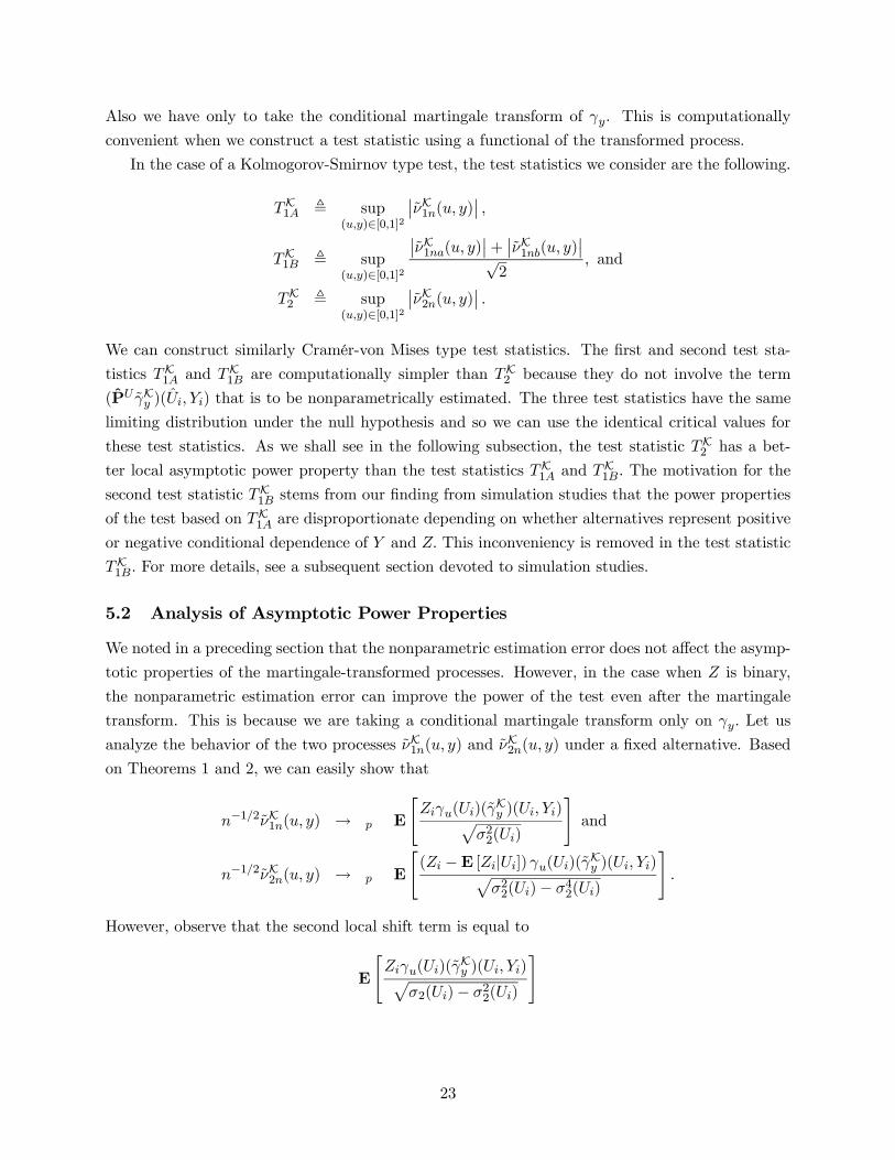
Also we have only to take the conditional martingale transform of γy. This is computationally

convenient when we construct a test statistic using a functional of the transformed process.

In the case of a Kolmogorov-Smirnov type test, the test statistics we consider are the following.

TK1A , sup(u,y)∈[0,1]2

¯νK1n(u, y)

¯,

TK1B , sup(u,y)∈[0,1]2

¯νK1na(u, y)

¯+¯νK1nb(u, y)

¯√2

, and

TK2 , sup(u,y)∈[0,1]2

¯νK2n(u, y)

¯.

We can construct similarly Cramér-von Mises type test statistics. The first and second test sta-

tistics TK1A and TK1B are computationally simpler than TK2 because they do not involve the term

(PU γKy )(Ui, Yi) that is to be nonparametrically estimated. The three test statistics have the same

limiting distribution under the null hypothesis and so we can use the identical critical values for

these test statistics. As we shall see in the following subsection, the test statistic TK2 has a bet-

ter local asymptotic power property than the test statistics TK1A and TK1B. The motivation for thesecond test statistic TK1B stems from our finding from simulation studies that the power properties

of the test based on TK1A are disproportionate depending on whether alternatives represent positiveor negative conditional dependence of Y and Z. This inconveniency is removed in the test statistic

TK1B. For more details, see a subsequent section devoted to simulation studies.

5.2 Analysis of Asymptotic Power Properties

We noted in a preceding section that the nonparametric estimation error does not affect the asymp-

totic properties of the martingale-transformed processes. However, in the case when Z is binary,

the nonparametric estimation error can improve the power of the test even after the martingale

transform. This is because we are taking a conditional martingale transform only on γy. Let us

analyze the behavior of the two processes νK1n(u, y) and νK2n(u, y) under a fixed alternative. Basedon Theorems 1 and 2, we can easily show that

n−1/2νK1n(u, y) → p E

"Ziγu(Ui)(γ

Ky )(Ui, Yi)p

σ22(Ui)

#and

n−1/2νK2n(u, y) → p E

"(Zi −E [Zi|Ui]) γu(Ui)(γ

Ky )(Ui, Yi)p

σ22(Ui)− σ42(Ui)

#.

However, observe that the second local shift term is equal to

E

"Ziγu(Ui)(γ

Ky )(Ui, Yi)p

σ2(Ui)− σ22(Ui)

#

23

because

E

"E [Zi|Ui] γu(Ui)(γ

Ky )(Ui, Yi)p

σ2(Ui)− σ22(Ui)

#= E

"E [Zi|Ui] γu(Ui)E

£(γKy )(Ui, Yi)|Ui

¤pσ2(Ui)− σ22(Ui)

#= 0.

by the conditional orthogonality condition for γKy . Since the denominator of the shift term for

νK1n(u, y) dominates that of the shift term for νK2n(u, y), the test based on the process νK2n(u, y) hasa better local asymptotic power than that based on n−1/2νK1n(u, y). This also shows the interestingphenomena that the test has a better power when we use the estimator (PU γKy )(Ui) for (PU γKy )(Ui)

instead of the true one. As before, we can formalize this phenomenon in terms of approximate

Bahadur ARE. Let e1,0(P1) be the approximate Bahadur ARE of the Kolmogorov-Smirnov test

base on νK1n(u, y) and that based on νK2n(u, y).

Corollary 4 : Suppose that the conditions of Theorem 1 hold except for that of Z. Then

e1,0(P1) =1

4.

This result is in contrast to that in the case with continuous Z and Y where no improvement of the

power was introduced by the nonparametric estimation error. The result of the improved power

property in Corollary 4 is demonstrated in the simulation studies.

5.3 Testing Procedure in Summary

In this subsection, we summarize the testing procedure for the case where Z is binary. First

we quantile-transform the data (Yi, λ(Xi))ni=1 to obtain (Yi, Ui)

ni=1. (We use the same notation Yi

here.) Then construct the test statistic in the following way. First estimate the conditional density

fY |U (y|u) using the data (Yi, Ui)ni=1 and the conditional distribution function FY |U (y|u) of Y given

U. Let us denote the estimated joint density by fY,U (y, u) and the conditional distribution function

by FY |U (y|u). Then we compute

αi(y, y) =1{Yi ≤ min(y, y)}q

fY,U (Yi, Ui)³1− FY |U (Y 0i |Ui)

´ .Note that our use of fY,U (Yi, Ui) instead of fY |U (Yi|Ui) is based on the fact that Ui is uniformly

distributed. Choose a basis function pK = (p1, p2, · · ·, pK)0. Let us define pK(u) = [p0(u), · · ·, pK(u)]0and define α(y, y) = [α1(y, y), · · ·, αn(y, y)]0. Then we define a K × 1 vector πn(y, y) by

πn(y, y) = [P0P ]−1P 0α(y, y).

The choice of K can be done using the procedure of cross-validations. We investigate the sensitivity

of the performance of tests to the choice of K in detail in the next section. Let P(Zi = 1|Ui) denote

24

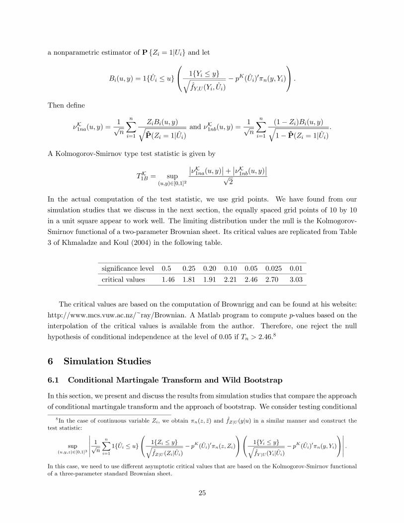
a nonparametric estimator of P {Zi = 1|Ui} and let

Bi(u, y) = 1{Ui ≤ u}⎛⎝ 1{Yi ≤ y}q

fY,U (Yi, Ui)− pK(Ui)

0πn(y, Yi)

⎞⎠ .

Then define

νK1na(u, y) =1√n

nXi=1

ZiBi(u, y)qP(Zi = 1|Ui)

and νK1nb(u, y) =1√n

nXi=1

(1− Zi)Bi(u, y)q1− P(Zi = 1|Ui)

.

A Kolmogorov-Smirnov type test statistic is given by

TK1B = sup(u,y)∈[0,1]2

¯νK1na(u, y)

¯+¯νK1nb(u, y)

¯√2

In the actual computation of the test statistic, we use grid points. We have found from our

simulation studies that we discuss in the next section, the equally spaced grid points of 10 by 10

in a unit square appear to work well. The limiting distribution under the null is the Kolmogorov-

Smirnov functional of a two-parameter Brownian sheet. Its critical values are replicated from Table

3 of Khmaladze and Koul (2004) in the following table.

significance level 0.5 0.25 0.20 0.10 0.05 0.025 0.01

critical values 1.46 1.81 1.91 2.21 2.46 2.70 3.03

The critical values are based on the computation of Brownrigg and can be found at his website:

http://www.mcs.vuw.ac.nz/~ray/Brownian. A Matlab program to compute p-values based on the

interpolation of the critical values is available from the author. Therefore, one reject the null

hypothesis of conditional independence at the level of 0.05 if Tn > 2.46.8

6 Simulation Studies

6.1 Conditional Martingale Transform and Wild Bootstrap

In this section, we present and discuss the results from simulation studies that compare the approach

of conditional martingale transform and the approach of bootstrap. We consider testing conditional

8 In the case of continuous variable Zi, we obtain πn(z, z) and fZ|U (y|u) in a similar manner and construct thetest statistic:

sup(u,y,z)∈[0,1]3

1√n

n

i=1

1{Ui ≤ u}⎛⎝ 1{Zi ≤ y}

fZ|U (Zi|Ui)− pK(Ui)

0πn(z, Zi)

⎞⎠⎛⎝ 1{Yi ≤ y}fY |U (Yi|Ui)

− pK(Ui)0πn(y, Yi)

⎞⎠ .

In this case, we need to use different asymptotic critical values that are based on the Kolmogorov-Smirnov functionalof a three-parameter standard Brownian sheet.

25

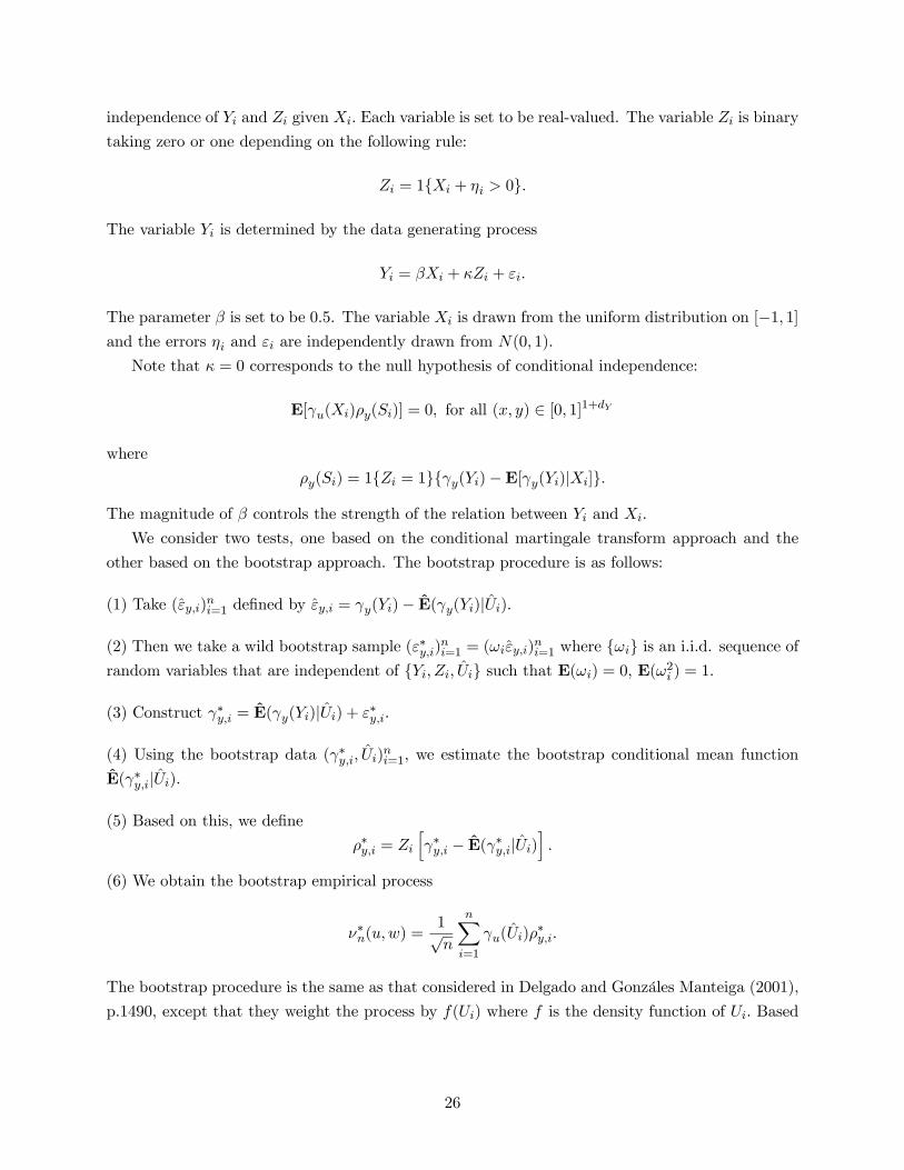
independence of Yi and Zi given Xi. Each variable is set to be real-valued. The variable Zi is binary

taking zero or one depending on the following rule:

Zi = 1{Xi + ηi > 0}.

The variable Yi is determined by the data generating process

Yi = βXi + κZi + εi.

The parameter β is set to be 0.5. The variable Xi is drawn from the uniform distribution on [−1, 1]and the errors ηi and εi are independently drawn from N(0, 1).

Note that κ = 0 corresponds to the null hypothesis of conditional independence:

E[γu(Xi)ρy(Si)] = 0, for all (x, y) ∈ [0, 1]1+dY

where

ρy(Si) = 1{Zi = 1}{γy(Yi)−E[γy(Yi)|Xi]}.

The magnitude of β controls the strength of the relation between Yi and Xi.

We consider two tests, one based on the conditional martingale transform approach and the

other based on the bootstrap approach. The bootstrap procedure is as follows:

(1) Take (εy,i)ni=1 defined by εy,i = γy(Yi)− E(γy(Yi)|Ui).

(2) Then we take a wild bootstrap sample (ε∗y,i)ni=1 = (ωiεy,i)

ni=1 where {ωi} is an i.i.d. sequence of

random variables that are independent of {Yi, Zi, Ui} such that E(ωi) = 0, E(ω2i ) = 1.

(3) Construct γ∗y,i = E(γy(Yi)|Ui) + ε∗y,i.

(4) Using the bootstrap data (γ∗y,i, Ui)ni=1, we estimate the bootstrap conditional mean function

E(γ∗y,i|Ui).

(5) Based on this, we define

ρ∗y,i = Zi

hγ∗y,i − E(γ∗y,i|Ui)

i.

(6) We obtain the bootstrap empirical process

ν∗n(u,w) =1√n

nXi=1

γu(Ui)ρ∗y,i.

The bootstrap procedure is the same as that considered in Delgado and Gonzáles Manteiga (2001),

p.1490, except that they weight the process by f(Ui) where f is the density function of Ui. Based

26

upon the bootstrap process, we can construct the bootstrap test statistics:

TBKS = sup

s∈[0,1]dY +1|ν∗n(u,w)| and TB

CM =

Z Zν∗n(u,w)

2dudw.

Nonparametric estimations are done using series-estimation with Legendre polynomials. We

rescale the variables Xi and Yi so that they have a unit interval support. The rescaling was

done by taking their (empirical) quantile transformations. We also take into account unknown

conditional heteroskedasticity by normalizing the semiparametric empirical process by σ(Ui)−1. The

test statistics are formed by using a Kolmogorov-Smirnov type. The number of Monte Carlo

iterations and the number of bootstrap Monte Carlo iterations are set to be 1000. The sample size

is 300.

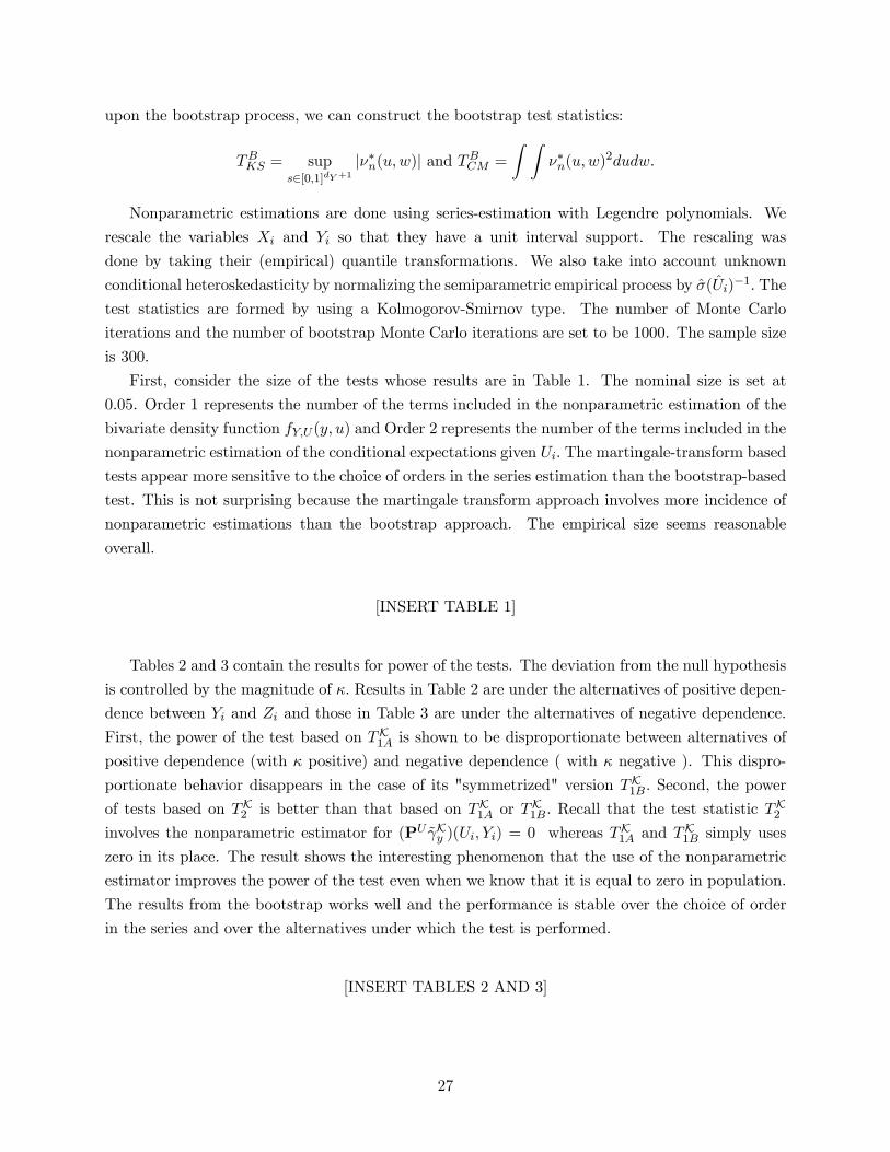
First, consider the size of the tests whose results are in Table 1. The nominal size is set at

0.05. Order 1 represents the number of the terms included in the nonparametric estimation of the

bivariate density function fY,U (y, u) and Order 2 represents the number of the terms included in the

nonparametric estimation of the conditional expectations given Ui. The martingale-transform based

tests appear more sensitive to the choice of orders in the series estimation than the bootstrap-based

test. This is not surprising because the martingale transform approach involves more incidence of

nonparametric estimations than the bootstrap approach. The empirical size seems reasonable

overall.

[INSERT TABLE 1]

Tables 2 and 3 contain the results for power of the tests. The deviation from the null hypothesis

is controlled by the magnitude of κ. Results in Table 2 are under the alternatives of positive depen-

dence between Yi and Zi and those in Table 3 are under the alternatives of negative dependence.

First, the power of the test based on TK1A is shown to be disproportionate between alternatives ofpositive dependence (with κ positive) and negative dependence ( with κ negative ). This dispro-

portionate behavior disappears in the case of its "symmetrized" version TK1B. Second, the powerof tests based on TK2 is better than that based on TK1A or T

K1B. Recall that the test statistic T

K2

involves the nonparametric estimator for (PU γKy )(Ui, Yi) = 0 whereas TK1A and TK1B simply uses

zero in its place. The result shows the interesting phenomenon that the use of the nonparametric

estimator improves the power of the test even when we know that it is equal to zero in population.

The results from the bootstrap works well and the performance is stable over the choice of order

in the series and over the alternatives under which the test is performed.

[INSERT TABLES 2 AND 3]

27

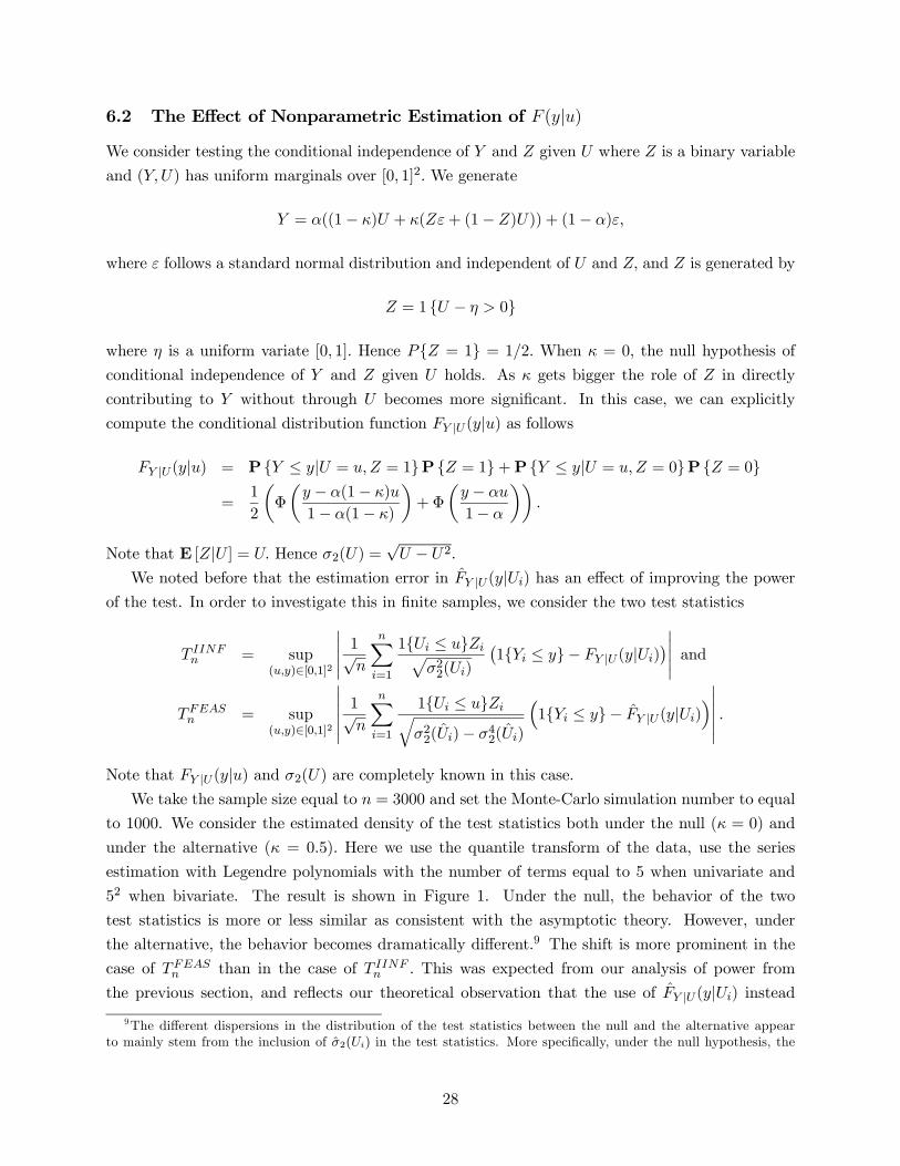
6.2 The Effect of Nonparametric Estimation of F (y|u)We consider testing the conditional independence of Y and Z given U where Z is a binary variable

and (Y,U) has uniform marginals over [0, 1]2. We generate

Y = α((1− κ)U + κ(Zε+ (1− Z)U)) + (1− α)ε,

where ε follows a standard normal distribution and independent of U and Z, and Z is generated by

Z = 1 {U − η > 0}

where η is a uniform variate [0, 1]. Hence P{Z = 1} = 1/2. When κ = 0, the null hypothesis of

conditional independence of Y and Z given U holds. As κ gets bigger the role of Z in directly

contributing to Y without through U becomes more significant. In this case, we can explicitly

compute the conditional distribution function FY |U (y|u) as follows

FY |U (y|u) = P {Y ≤ y|U = u,Z = 1}P {Z = 1}+P {Y ≤ y|U = u,Z = 0}P {Z = 0}

=1

2

µΦ

µy − α(1− κ)u

1− α(1− κ)

¶+Φ

µy − αu

1− α

¶¶.

Note that E [Z|U ] = U. Hence σ2(U) =√U − U2.

We noted before that the estimation error in FY |U(y|Ui) has an effect of improving the power

of the test. In order to investigate this in finite samples, we consider the two test statistics

T IINFn = sup

(u,y)∈[0,1]2

¯¯ 1√n

nXi=1

1{Ui ≤ u}Zipσ22(Ui)

¡1{Yi ≤ y}− FY |U (y|Ui)

¢¯¯ andTFEASn = sup

(u,y)∈[0,1]2

¯¯ 1√n

nXi=1

1{Ui ≤ u}Ziqσ22(Ui)− σ42(Ui)

³1{Yi ≤ y}− FY |U (y|Ui)

´¯¯ .Note that FY |U (y|u) and σ2(U) are completely known in this case.

We take the sample size equal to n = 3000 and set the Monte-Carlo simulation number to equal

to 1000. We consider the estimated density of the test statistics both under the null (κ = 0) and

under the alternative (κ = 0.5). Here we use the quantile transform of the data, use the series

estimation with Legendre polynomials with the number of terms equal to 5 when univariate and

52 when bivariate. The result is shown in Figure 1. Under the null, the behavior of the two

test statistics is more or less similar as consistent with the asymptotic theory. However, under

the alternative, the behavior becomes dramatically different.9 The shift is more prominent in the

case of TFEASn than in the case of T IINF

n . This was expected from our analysis of power from

the previous section, and reflects our theoretical observation that the use of FY |U (y|Ui) instead

9The different dispersions in the distribution of the test statistics between the null and the alternative appearto mainly stem from the inclusion of σ2(Ui) in the test statistics. More specifically, under the null hypothesis, the

28

of FY |U (y|Ui) improves the local power properties of the tests. This is also observed in terms of

empirical processes inside T IINFn and TFEAS

n as shown in Figure 2.

[INSERT FIGURES 1 AND 2]

7 Conclusion

A test of conditional independence has been proposed. The test is asymptotically unbiased against

Pitman local alternatives and yet has critical values that can be tabulated from the limiting distri-

bution theory. As in Song (2006b), the main idea is to employ conditional martingale transforms,

but the manner that we apply the transforms in testing conditional independence is different. We

apply the transform to the indicator functions of Zi and Yi with the conditioning on Ui.

There are two possible extensions: first, the analysis of the asymptotic power function, and

second, the accommodation of weakly dependent data. The analysis of the asymptotic power

function will illuminate the effect of the martingale transform on the power of the tests. The i.i.d.

assumption in testing conditional independence is restrictive considering that testing the presence

of causal relations often presupposes the context of time series. Extending the results in the paper

to time series appears nontrivial because the methods of this paper heavily draws on the results of

empirical process theory that are based on independent series. However, there have been numerous

efforts in the literature to extend the results of empirical processes to time series (e.g., Andrews

(1991), Arcones and Yu (1994), and Nishyama (2000).) It seems that the results in this paper can

be extended to time series context based on those results.

covariance kernel of the process

1√n

n

i=1

1{Ui ≤ u}Ziσ2(Ui)

1{Yi ≤ y}− FY |U (y|Ui)

is equal tou1∧u2

0

FY |U (y1 ∧ y2|u)− FY |U (y1|u)FY |U (y2|u) du

whereas under the Pitman local alternatives, the process is asymptotically equivalent to a shifted version of thefollowing process

1√n

n

i=1

1{Ui ≤ u}σ2(Ui)

(Zi1{Yi ≤ y}−E [Zi1{Yi ≤ y}|Ui])) .

The covariance kernel of this process is equal to

u1∧u2

0

Φ(u)−2 {E [Zi1{Yi ≤ y1 ∧ y2}|Ui = u]−E [Zi1{Yi ≤ y1}|Ui = u]E [Zi1{Yi ≤ y2}|Ui = u]} du

=u1∧u2

0

Φ(u)−2 Φ(u)FY |U (y1 ∧ y2|u)−Φ(u)2FY |U (y1|u)FY |U (y2|u) du

=u1∧u2

0

Φ−1(u)FY |U (y1 ∧ y2|u)− FY |U (y1|u)FY |U (y2|u)

since σ2(U) = P (Z = 1|U) = Φ(U). Since Φ(U) ∈ [0, 1], the covariance kernel above dominates that of the processunder the null hypothesis.

29

8 Appendix: Mathematical Proofs

8.1 Main Results

We first prove Theorem 1. The following lemma is useful for this end. Define

γu,n,λ(x) , 1(1

n

nXi=1

1 {λ(Xi) ≤ λ(x)} ≤ u

).

The function γu,n,λ(·) is indexed by (u, λ) ∈ [0, 1] × Λn. The indicator function contains the non-parametric function which is an empirical distribution function. Note that we cannot directly apply

the framework of Chen, Linton and van Keilegom (2003) to analyze the class of functions that the

realizations of γu,n,λ(x) falls into. This is because when the indicator function contains a non-

parametric function, the procedure of Chen, Linton, and van Keilegom (2003) requires the entropy

condition for the nonparametric functions with respect to the sup norm. This entropy condition

with respect to the sup norm does not help because Lp uniform continuity fails with respect to the

sup norm. Hence we establish the following result for our purpose.

Lemma A1 : There exists a sequence of classes Gn of measurable functions such that

P©γu,n,λ ∈ Gn for all (u, λ) ∈ [0, 1]× Λn

ª= 1,

and for any r ≥ 1,

logN[](C2ε,Gn, || · ||r) ≤ logN(εr/2,Λn, || · ||∞) +C1ε,

where C1 and C2 are positive constants depending only on r.

Proof of Lemma A1 : For a fixed sequence {xi}ni=1 with {xi} ∈ RndX , we define a function:

gn,λ,u(λ) , 1(1

n

nXi=1

1©λ(xi) ≤ λ

ª ≤ u

),

where gn,λ,u(·) depends on the chosen sequence {xi}ni=1 .We introduce classes of functions as follows:

G0n ,ngn,λ,u : (λ, {xi}ni=1, u) ∈ Λn ×RndX × [0, 1]

oand

Gn ,©g ◦ λ : (g, λ) ∈ G0n × Λn

ª.

Then we have γu,n,λ ∈ Gn. Note that gn,λ,u(λ) is decreasing in λ. Hence by Theorem 2.7.5 in van

der Vaart and Wellner (1996), for any r ≥ 1

logN[](ε,G0n, || · ||Q,r) ≤C1ε, (21)

30

for any probability measure Q and for some constant C1 > 0.

Without loss of generality, assume that λ(X) ∈ [0, 1]. We choose {λ1, · · ·, λN2} such that forany λ ∈ Λn, there exists j with kλj − λk∞ < εr/2. For each j, we define λj(x) as follows.

λj(x) = mεr/2 when λj(x) ∈ [mεr/2, (m+ 1)εr/2) for some m ∈ {0, 1, 2, · · ·, b2/εrc},

where bzc denotes the greatest integer that does not exceed z. Note that the range of λj is finite

and

||λ− λj ||∞ = supx

b2/εrcXk=0

|λ(x)− kεr/2| 1 {λj(x) ∈ [kεr/2, (k + 1)εr/2)}

≤ supx

b2/εcXk=0

(|λ(x)− λj(x)|+ |λj(x)− kεr/2|) 1 {λj(x) ∈ [kεr/2, (k + 1)εr/2)} ≤ εr.

From (21), we have logN(ε,G0n, || · ||Q,r) ≤ C1/ε.We choose {g1, · · ·, gN1} such that for any g ∈ G0n,there exists j such that

R |g(u)− gj(u)|rdu < εr. Then we have for any λ ∈ Λn,

E |g(λ(X))− gj(λ(X))|r =Z ¯

g(λ)− gj(λ)¯rfλ(λ)du ≤ sup

λsupλ

f(λ)εr,

where fλ(·) denotes the density of λ(X).Now, take any h ∈ Gn such that h , g ◦ λ and choose (gj1 , λj2) from {g1, · · ·, gN1} and

{λ1, · · ·, λN2} such that Z|g(u)− gj1(u)|rdu < εr and kλj2 − λk∞ < εr/2.

Then consider°°°h− gj1 ◦ λj2°°°r≤ kg ◦ λ− gj1 ◦ λkr +

°°°gj1 ◦ λ− gj1 ◦ λj2°°°r

≤µsupλsupλ

f(λ)

¶1/rε+

³E¯(gj1 ◦ λ)(X)− (gj1 ◦ λj2)(X)

¯r´1/r.

Note that the absolute value in the expectation of the second term is bounded by

1

(1

n

nXi=1

1nλj1(xi) ≤ λj2(X)− εr

o≤ uj1

)− 1

(1

n

nXi=1

1nλj1(xi) ≤ λj2(X) + εr

o≤ uj1

)

31

or by

1

(1

n

nXi=1

1nλj1(xi) ≤ λj2(X)− εr

o≤ uj1 <

1

n

nXi=1

1nλj1(xi) ≤ λj2(X) + εr

o)

=

b2/εcXm=0

1

(1

n

nXi=1

1

½λj1(xi) ≤

mεr

2− εr

¾≤ uj1 <

1

n

nXi=1

1

½λj1(xi) ≤

mεr

2+ εr

¾)

×1½mεr

2≤ λj2(X) <

(m+ 1)εr

2

¾.

Each summand in the last sum, as a range of a fixed value uj1 , overlaps with precisely three other

adjacent ones, and hence is bounded by

1 {λj2(X) ∈ [kεr/2, (k + 3)εr/2)}

for some k ∈ {0, 1, 2, · · ·, b2/εrc}. By taking expectation, this last indicator function is bounded by

P {λj2(X) ∈ [mεr/2, (m+ 2)εr/2)} = Fλj2 ((m+ 2)εr/2)− Fλj2 (mεr/2)

≤ supλ

fλj2 (λ)εr,

where Fλj2 is the distribution function of λj2(X). Therefore,°°°h− gj1 ◦ λj2°°°r≤ 2

µsupλsupλ

fλ(λ)

¶1/rε.

This leads to the result that

logN[]

Ã2

µsupλsupλ

fλ(λ)

¶1/rε,Gn, || · ||r

!≤ logN(εr/2,Λn, || · ||∞) + logN[](ε,G0n, || · ||r)

≤ logN(εr/2,Λn, || · ||∞) + C

ε.

We define two notations that we use throughout the remaining proofs. First, P denotes the op-eration of sample mean: Pf , 1

n

Pni=1 f(Si) and second,

⊥ denotes the conditional mean deviation:γ⊥y (Y,U) , γy(Y )−E

£γy(Y )|U = u

¤.

Proof of Theorem 1 : Recall that

νn(r) =1√n

nXi=1

γu(Ui)γz(Zi)©γy(Zi)−E(γy(Zi)|Ui)

ª=√nPγuγz(γ⊥y ).

Then we analyze the asymptotic behavior of the empirical process above under the null hypothesis

and under the alternatives. Choose a sequence λ within the shrinking neighborhood B(λ0, δn) ⊂ Λ

32

of λ0 with diameter δn = o(1) in terms of || · ||2. Consider

(PUλγ)(u) , pK(u)0πγ,λ,

where πγ,λ , [P 0λPλ]−1P 0

λyγ,n with yγ,n and Pλ being defined by

yγ,n ,

⎡⎢⎢⎣γ(Y1)...

γ(Yn)

⎤⎥⎥⎦ and Pλ ,

⎡⎢⎢⎣pK(Un,λ(X1))

0...

pK(Un,λ(Xn))0

⎤⎥⎥⎦ .Note that PU

λis the same as PU except that λ is replaced by λ.

We define a process νn(g, r, λ) indexed by (g, r, λ) ∈ Gn × [0, 1]dr × Λn as

νn(g, r, λ) ,1√n

nXi=1

g(Xi)γz(Zi)hγy(Yi)− pK(Un,λ(Xi))

0πγ,λi.

Then by Lemma 1U of Escanciano and Song (2006), we obtain the result that νn(g, r, λ) is equal

to1√n

nXi=1

[g(Xi)γz(Zi)−E [g(Xi)γz(Zi)|Ui]£γy(Yi)−P {Yi ≤ y|Ui}

¤+ oP (1)

where oP (1) is uniform over (g, r, λ) ∈ Gn × [0, 1]dr × Λn. Hence the above holds for any arbitrarysequence gn ∈ Gn such that gn → γu. Since γu(Ui) is a function of Ui, this yields the result.

Proof of Corollary 1 : (i) Assume the null hypothesis. We first consider ν1n(r). The con-

vergence of finite dimensional distributions of the process√nPn

£γuγ

⊥z γ

⊥y

¤follows by the usual

CLT. Note that the finite second moment condition trivially follows from the uniform bounded-

ness of the indicator functions. And it is trivial to compute the covariance function of the process√nPn[γuγz⊥γy⊥] to verify the covariance function of the limit Gaussian process in the theorem.

Since the rectangle [0, 1]3 is obviously totally bounded with respect to the Euclidean norm, it re-

mains to show that the process√nPna is stochastically equicontinuous in a ∈ A where A is defined

by {γu(γz)⊥(γy)⊥ : (u, z, y) ∈ [0, 1]3}. However, it is well-known that the class of univariate in-dicator functions is VC and products of a finite number of the indicator functions are also VC

by the stability properties of VC classes (see van der Vaart and Wellner(1996)). Hence the re-

quired stochastic equicontinuity follows. Therefore we obtain the wanted result. It is a trivial

matter to check the covariance kernel. We can likewise analyze the limit behavior of the process

νn(r) =√nPn

£γuγzγ

⊥y

¤to obtain the wanted result.

(ii) First consider νn(r) which we write

νn(r) = Pnhγuγzγ

⊥y

i= Pnγu

hγzγ

⊥y

i⊥+ Pn[γu[PUρw]−P{γu[PUρw]}] +P[γuρw],

33

where ρw , γz(γy−PUγy). Now, assume that the null hypothesis does not necessarily hold. Using

the preliminary result in (6), we write

νn(r) = Pnhγuγ

⊥z γ

⊥y

i+ oP (1)

= Pnγuhγ⊥z γ

⊥y

i⊥+ Pn[γu[PUρw]−P{γu[PUρw]}] +P[γuρw] + oP (1)

by adding and subtracting terms. The first and second process is a mean-zero empirical process,

and using the similar arguments in (i), it is not hard to show that the processes are indexed by a

Glivenko-Cantelli class. Hence, the result follows.

Proof of Theorem 2 (i) The proof is similar to the proof of Proposition 6.1 of Khmaladze andKoul (2004).

(ii) (a) We apply Theorem 1 to the process

νKn (r) =1√n

nXi=1

γu(Ui)γKz (Zi){γKy (Yi)− (PUγKy )(Yi, Ui)}

by replacing γz and γy by γKz and γ

Ky . In view of the proof of Theorem 1, the main step is applying

Lemma 1U of Escanciano and Song (2006) to the above process. To this end, it suffices to show that

the classes {γKy : y ∈ [0, 1]} and {γKz : z ∈ [0, 1]} satisfy the required bracketing entropy conditions.This is shown in Lemma A2 below. Hence by following the same steps in the proof of Theorem 1,

we obtain that under the null hypothesis,

νKn (r) =√nPn[γu(γKz )⊥(γKy )⊥] + oP (1). (22)

Furthermore, by observing from (i) of this theorem,

PU (γKy ) = 0 and PU (γKz ) = 0,

Note that under the null hypothesis of conditional independence, (γKz )(Ui, Zi) and (γKy )(Ui, Yi) are

conditionally independent given Ui. Therefore

PU (γKz γKy ) = P

U (γKz )PU (γKy ) = 0.

Therefore, under the null hypothesis, we have

νKn (r) =√nPn[γu(γKz )(γKy )] + oP (1).

We investigate the process√nPn[γu(γKz )(γKy )] and establish its weak convergence. The con-

vergence of finite dimensional distributions follows by the usual central limit theorem. Note that

the functions γKy and γKz are uniformly bounded. By Lemma A2, the process√nPn[γu(γKz )(γKy )]

is stochastically equicontinuous in S0 and the index space S0 is totally bounded with respect to

34

the Euclidean norm in [0, 1]3, the weak convergence of the process√nPn[γu(γKz )(γKy )] follows by

Proposition in Andrews (1994), p. 2251.

The covariance function of the process is equal to

P£γu1∧u2(γ

Kz1)(γ

Kz2)(γ

Ky1)(γ

Ky2)¤. (23)

It is easy to see that under the null hypothesis of conditional independence, the covariance function

becomes

P£γu1∧u2P

U£(γKz1)(γ

Kz2)(γ

Ky1)(γ

Ky2)¤¤

= P£γu1∧u2P

U£γKz1γ

Kz2

¤PU

£γKy1γ

Ky2

¤¤= P

£γu1∧u2P

U£γz1γz2

¤PU

£γy1γy2

¤¤= P

£γu1∧u2γz1∧z2γy1∧y2

¤.

By the null hypothesis of conditional independence, the above is equal toZ u1∧u2FZ|U (z1 ∧ z2|u)FY |U (y1 ∧ y2|u)dF (u).

Now, when we replace γKu , γKz , and γKy by γKu , γKz , and γKy , the covariance function becomesZ u1∧u2f−1(u)

∙Z z1∧z2f−1Z|U (z|u)fZ|U (z|u)dz

¸ ∙Z y1∧y2f−1Y |U (y|u)fY |U (y|u)dy

¸f(u)du

= (u1 ∧ u2)(z1 ∧ z2)(y1 ∧ y2).

(b) The result is immediate from (22).

We introduce notations for classes of functions:

GKY , {γKy : y ∈ [0, 1]} and GKu,y , {PUγKz : z ∈ [0, 1]}.

The following result provides the bracketing entropy bound for these classes. The result implies

that these classes are P -Donsker.

Lemma A2 : Suppose the conditions of Theorem 2 holds. Then we have for p ≥ 2,

N[](ε,GKY , || · ||p) ≤ C1ε−2p and N[](ε,GKu,y, || · ||p) ≤ C2ε

−2p.

Proof : Define GY , {γy : y ∈ [0, 1]}. Then we have (e.g. the proof of Lemma A1(d) in Song(2006b)), N[](ε,GY , || · ||p) ≤ 2ε−p. Now, recall that

(Muγy)(u, y) , (PUγy∧yH)(u), where H(y, u) ,1

1− FY |U (y;u).

From the previous observation, for the class G0Y , {γy∧y(·)/(1 − FY |U (·; ·)) : (y, y) ∈ [0, 1]2}, we

35

have N[](ε,G0Y , || · ||p) ≤ Cε−p and hence for the class G00Y , {PUg : g ∈ G0Y }, we also haveN[](ε,G00Y , || · ||p) ≤ Cε−p. Note that the denominator of (1 − FY |U (·; ·)) does not depend on theindex (y, y)2 ∈ [0, 1]2. Hence

N[](Cε,GKY , || · ||p) ≤ N[](ε,GY , || · ||p)×N[](ε,G00Y , || · ||p) ≤ Cε−2p.

From this, the second statement N[](ε,GKu,y, || · ||p) ≤ C2ε−2p immediately follows.

Proof of Corollary 2 : The covariance kernels of the limit Gaussian processes of ν(r) and ν1(r)

in Theorem 1 are respectively given by

c(r1, r2) = (u1 ∧ u2)(z1 ∧ z2)(y1 ∧ y2 − y1y2),

c1(r1, r2) = (u1 ∧ u2)(z1 ∧ z2 − z1z2)(y1 ∧ y2 − y1y2).

Therefore, (e.g. Lemma 4.8.1 in Nikitin (1995)) we have

limκ→∞κ−2 logP

(sup

r∈[0,1]dr|ν(r)| ≥ κ

)= −1

2b0

limκ→∞κ−2 logP

(sup

r∈[0,1]dr|ν1(r)| ≥ κ

)= −1

2b1,

where the constants b0 and b1 are given by

b−10 = supr∈[0,1]3

c(r, r) =1

4and b−11 = sup

r∈[0,1]3c1(r, r) =

1

16.

Now let us consider the case of alternatives. The results of Theorem 1 yields that the function

ϕ0 and ϕ1 in (8) are equal, given by

ϕ0(r) = P1£γu(hγz, γyiU − hγz, 1iU hγy, 1iU )

¤.

Therefore, we obtain the result of the approximate Bahadur efficiency e0,1(P1).

Proof of Corollary 3 : (i) The covariance kernels of the limit Gaussian processes of νK(r) isgiven by

cK(r1, r2) = (u1 ∧ u2)(z1 ∧ z2)(y1 ∧ y2),

yielding the result that (e.g. Lemma 4.8.1 in Nikitin (1995)) we have

limκ→∞κ−2 logP

(sup

r∈[0,1]dr|νK(r)| ≥ κ

)= −1

2bK,

where the constant bK is given by b−1K = supr∈[0,1]dr cK(r, r) = 1. On the other hand, under P1, we

36

have

ϕ0(r) = E1£γu{hγz, γyiU − hγz, 1iU hγy, 1iU}

¤= E1

£γu(U)

©CZ,Y |U (FZ|U (z|U), FY |U (y|U)|U)− FZ|U (z|U)FY |U (y|U)

ª¤.

Now, we turn to ϕK(r). Observe that

ϕK(r) = P1£γu(hγKz , γKy iU − hγKz , 1iU hγKy , 1iU)

¤(24)

= P1£γuhγKz , γKy iU

¤= E1

£(Kγz)(U ;Z)(Kγy)(U ;Y )|U

¤.

The second equality follows from the conditional orthogonality property of K.First, assume without loss of generality that ξ(z, ε) is strictly increasing in z. We observe that

the last term in (24) is equal to

E1

h(Kγz)(U ;Z)(Kγξ−1(y,ε))(U ;Z)|U

i(25)

in this case. (When ξ(z, ε) is strictly decreasing in z, the last term in (24) is equal to

E1

h(Kγz)(U ;Z)(K(1− γξ−1(y,ε)))(U ;Z)|U

i= −E1

h(Kγz)(U ;Z)(Kγξ−1(y,ε))(U ;Z)|U

i,

because K is a linear operator and Ka = 0 for any constant a. Then we can follow the subsequentsteps in a similar manner.) By the conditional isometry condition, the term in (25) is equal to

E1

hγz(Z)γξ−1(y,ε)(Z)|U

i= E1

£FZ|U

¡z ∧ ξ−1 (y, ε) |U¢ |U¤

= P©Z ≤ z, Z ≤ ξ−1 (y, ε) |Uª

= CZ,Y |U (FZ|U (z|U), FY |U (y|U)|U).

Therefore,

Γϕ0 = supz,y,u

¯E£γu(U)

©CZ,Y |U(FZ|U (z|U), FY |U (y|U)|U)− FZ|U (z|U)FY |U (y|U)

ª¤¯= sup

z,y

¯E£CZ,Y |U (FZ|U (z|U), FY |U (y|U)|U)− FZ|U (z|U)FY |U (y|U)

¤¯ΓϕK = sup

z,y,uE£γu(U)CZ,Y |U(FZ|U (z|U), FY |U (y|U)|U)

¤= sup

z,yE£CZ,Y |U (FZ|U(z|U), FY |U (y|U)|U)

¤

37

Combining the results, we obtain the first statement.

e1,K(P1) =4 supz,y

¯E£CZ,Y |U (FZ|U (z|U), FY |U (y|U)|U)− FZ|U (z|U)FY |U (y|U)

¤¯supz,y E

£CZ,Y |U (FZ|U (z|U), FY |U (y|U)|U)

¤= 4 sup

z,y

¯E£CZ,Y |U (FZ|U (z|U), FY |U (y|U)|U)− FZ|U (z|U)FY |U (y|U)

¤¯.

The last equality follows as the supremum in the denominator is achieved when z = y = 1.

(ii) Write the approximate Bahadur ARE as

e1,K(P1) = 4 supz,y

¯E£CZ,Y |U (FZ|U (z|U), FY |U (y|U)|U)

¤−E £FZ|U (z|U)FY |U (y|U)¤¯= 4 sup

z,y

¯CZ,Y (z, y)−E

£FZ|U (z|U)FY |U (y|U)

¤¯.

First, we assume that ξ(z, ε) is strictly increasing in z. Then

E£FZ|U (z|U)FY |U (y|U)

¤− zy

= E£FZ|U (z|U)FY |U (y|U)

¤−E £FZ|U (z|U)¤E £FY |U (y|U)¤ ≥ 0because FZ|U (z|U) and FY |U (y|U) are nonnegatively correlated. Hence take h(z, y) , z ∧ y −CZ,Y (z, y) ≥ 0 and observe

e1,K(P1) ≤ 4 supz,y{CZ,Y (z, y)− zy} ≤ 4 sup

z,y{CZ,Y (z, y) + h(z, y)− zy}

= 4 supz,y{z ∧ y − zy} = 1.

The last equality follows as the supremum is achieved by z = y = 1/2.

Now, assume that ξ(z, ε) is strictly decreasing in z. Then FZ|U (z|U) and FY |U (y|U) are non-positively correlated and we have

E£FZ|U(z|U)FY |U (y|U)

¤− zy ≤ 0.

We take h(z, y) = CZ,Y (z, y) − max{z + y − 1, 0} ≥ 0. Since Z and Y are negatively dependent

conditional on U , CZ,Y (z, y)−E£FZ|U (z|U)FY |U (y|U)

¤ ≤ 0 and hencee1,K(P1) = 4 sup

z,y

©E£FZ|U (z|U)FY |U (y|U)

¤− CZ,Y (z, y)ª

≤ 4 supz,y{zy − CZ,Y (z, y)} ≤ 4 sup

z,y{zy + h(z, y)− CZ,Y (z, y)}

= 4 supz,y{zy −max{z + y − 1, 0}} = 1.

Proof of Corollary 4 : The covariance kernels of the limit Gaussian processes of νK(r) and νK1 (r)

38

in Theorem 1 are respectively given by

cK(r1, r2) = C(u1 ∧ u2)(y1 ∧ y2),c1,K(r1, r2) = C(u1 ∧ u2)(y1 ∧ y2 − y1y2).

Therefore, (e.g. Lemma 4.8.1 in Nikitin (1995)) we have

limκ→∞κ−2 logP

(sup

r∈[0,1]3¯νK(r)

¯ ≥ κ

)= −1

2b0

limκ→∞κ−2 logP

(sup

r∈[0,1]3¯νK1 (r)

¯ ≥ κ

)= −1

2b1,

where the constants b0 and b1 are given by

b−10 = supr∈[0,1]3

cK(r, r) = 1 and b−11 = supr∈[0,1]3

c1,K(r, r) =1

4.

Now let us consider the case of alternatives. The results of Theorem 1 yields that the function

ϕ0 and ϕ1 in (8) are equal, given by

ϕ0(r) = E£Zγu(U)(γ

Ky )(U, Y )

¤.

Therefore, we obtain the result of the approximate Bahadur efficiency e0,1(P1).

39

References

[1] Ai, C. and X. Chen (2003), "Efficient estimation of models with conditional moment restric-

tions containing unknown functions," Econometrica 71, 1795-1843.

[2] Altonji, J. and R. Matzkin (2005), "Cross-section and panel data estimators for nonseparable

models with endogenous regressors," Econometrica 73, 1053-1102.

[3] Andrews, D. W. K (1991), "An empirical process central limit theorem for dependent non-

identically distributed random variables," Journal of Multivariate Analysis, 38, 187-203.

[4] Andrews, D. W. K (1994), “Empirical process method in econometrics,” in The Handbook of

Econometrics, Vol. IV, ed. by R. F. Engle and D. L. McFadden, Amsterdam: North-Holland.

[5] Andrews, D. W. K (1995), "Nonparametric kernel estimator for semiparametric models,"

Econometric Theory, 11, 560-595.

[6] Andrews, D. W. K (1997), “A conditional Kolmogorov test,” Econometrica, 65, 1097-1128.

[7] Angrist, J. D. and G. M. Kuersteiner (2004), "Semiparametric causality tests using the policy

propensity score," Working paper.

[8] Arcones, M. A. and B. Yu (1994), "Central limit theorems for empirical and U-processes of

stationary mixing sequences," Journal of Theoretical Probability, 7, 47-71.

[9] Bahadur, R. R. (1960), "Stochastic comparison of tests," Annals of Mathematical Statistics,

31, 276-295.

[10] Bierens, H. J. (1990), “A consistent conditional moment test of functional form,” Econometrica

58, 1443-1458.

[11] Bierens, H. J. and W. Ploberger, (1997), “Asymptotic theory of integrated conditional moment

tests,” Econometrica 65, 1129-1151.

[12] Chen, X., O. Linton, and I. van Keilegom (2003), "Estimation of semiparametric models when

the criterion function is not smooth," Econometrica 71, 1591-1608.

[13] Chen, X., and X. Shen (1998), "Sieve extremum estimates for weakly dependent data," Econo-

metrica, 66, 289-314.

[14] Chung, K. L. (2001), A Course in Probability Theory, Academic Press, 3rd Ed.

[15] Dawid, P. (1980), "Conditional independence for statistical operations," Annals of Statistics,

8, 598-617.

[16] Delgado, M. A., W. Gonzáles Manteiga (2001), "Significance testing in nonparametric regres-

sion based on the bootstrap," Annals of Statistics 29, 1469-1507.

40

[17] Escanciano, J. C. and K. Song (2006), "Asymptotically optimal tests for single index restric-

tions with a focus on average partial effects," Working paper.

[18] Fan, Y. and Q. Li (1996), “Consistent model specification tests: omitted variables, parametric

and semiparametric functional forms,” Econometrica, 64, 865-890.

[19] Härdle, W. and E. Mammen (1993), “Comparing nonparametric versus parametric regression

fits,” Annals of Statistics, 21, 1926-1947.

[20] Hirano, K., G. W. Imbens, and G. Ridder (2003), "Efficient estimation of average treatment

effects using the estimated propensity score," Econometrica, 71, 1161-1189.

[21] Khmaladze, E. V. (1993), “Goodness of fit problem and scanning innovation martingales,”

Annals of Statistics, 21, 798-829.

[22] Khmaladze, E. V. and H. Koul (2004), “Martingale transforms goodness-of-fit tests in regres-

sion models,” Annals of Statistics, 32, 995-1034.

[23] Linton, O. and P. Gozalo (1997), "Conditional independence restrictions: testing and estima-

tion", Cowles Foundation Discussion Paper 1140.

[24] McKeague, I. W. and Y. Sun (1996), “Transformations of gaussian random fields to Brownian

sheet and nonparametric change-point tests,” Statistics and Probability Letters, 28, 311-319.

[25] Nelsen, R. B. (1999), An Introduction to Copulas, Springer-Verlag, New York

[26] Newey, W. K. (1997), "Convergence rates and asymptotic normality of series estimators,"

Journal of Econometrics, 79, 147-168.

[27] Nikitin, Y. (1995), Asymptotic Efficiency of Nonparametric Tests, Cambridge University Press,

New York.

[28] Nishiyama, Y. (2000), Entropy methods for martingales, CWI Tract, 128.

[29] Rosenbaum, P. and D. Rubin (1983), "The central role of the propensity score in observational

studies for causal effects," Biometrika, 70, 41-55.

[30] Patton, A. (2006), "Modeling asymmetric exchange rate dependence," International Economic

Review, 47, 527-556.

[31] Rosenblatt, M. (1952), "Remarks on a multivariate transform," Annals of Mathematical Sta-

tistics, 23, 470-472.

[32] Rubin, D. "Bayesian inference for causal effects: the role of randomization," Annals of Statis-

tics, 6, 34-58.

41

[33] Song, K. (2006a), "Uniform convergence of series estimator over functional spaces," Working

paper.

[34] Song, K. (2006b), "Testing semiparametric conditional moment restrictions using conditional

martingale transforms," Working Paper.

[35] Stinchcombe, M. B. and H. White (1998), "Consistent specification testing with nuisance

parameters present only under the alternative," Econometric Theory, 14, 295-325.

[36] Stute, W. and L. Zhu (2005), “Nonparametric checks for single-index models,” Annals of

Statistics, 33, 1048-1083.

[37] Su, L. and H. White (2003a), "Testing conditional independence via empirical likelihood,"

Discussion Paper, University of California San Diego.

[38] Su, L. and H. White (2003b), "A nonparametric Hellinger metric test for conditional indepen-

dence," Discussion Paper, University of California San Diego.

[39] Su, L. and H. White (2003c), "A characteristic-function-based test for conditional indepen-

dence," Discussion Paper, University of California San Diego.

[40] van der Vaart, A. W. and J. A. Wellner (1996), Weak Convergence and Empirical Processes,

Springer-Verlag.

42

Table 1 : Size of the Tests : Nominal size is set at 5 Percent 10

n = 300

Order 1 Order 2 MG trns (TK1A) MG trns (TK1B) MG trns (TK2 ) Bootstrap

4 0.034 0.054 0.061 0.060

42 5 0.050 0.077 0.076 0.055

6 0.058 0.072 0.073 0.056

7 0.076 0.118 0.088 0.055

4 0.050 0.044 0.070 0.039

52 5 0.037 0.064 0.059 0.056

6 0.059 0.099 0.078 0.046

7 0.090 0.120 0.115 0.042

4 0.035 0.040 0.055 0.050

62 5 0.032 0.068 0.057 0.055

6 0.054 0.092 0.085 0.056

7 0.070 0.106 0.096 0.049

4 0.041 0.048 0.067 0.061

72 5 0.047 0.073 0.066 0.051

6 0.062 0.084 0.082 0.048

7 0.080 0.121 0.089 0.055

10Order 1 represents the number of terms included in the bivariate density function estimation using Legendrepolynomials. Order 2 represents the number of terms included in the estimation of conditional expectation given Uiusing Legendre polynomials.MG trns (TK1A) and MG trns (T

K2 ) indicate tests based on martingale transforms, the former using the test statistic

TK1A which is based on the true conditional expectation of γKy (Y ) given U and the latter using the test statistic TK2

which is based on the estimated conditional expectation of γKy (Y ) given U. MG trns (TK1B) is the symmetrized version

of MG trns (TK1A).

43

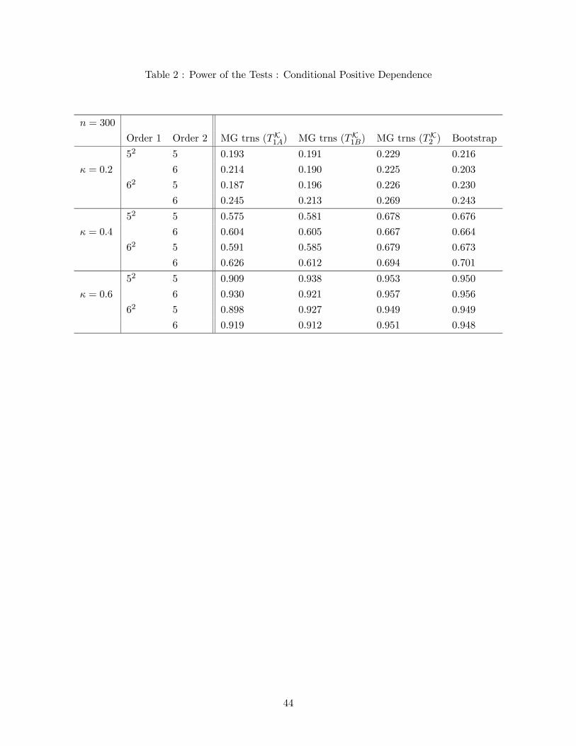
Table 2 : Power of the Tests : Conditional Positive Dependence

n = 300

Order 1 Order 2 MG trns (TK1A) MG trns (TK1B) MG trns (TK2 ) Bootstrap

52 5 0.193 0.191 0.229 0.216

κ = 0.2 6 0.214 0.190 0.225 0.203

62 5 0.187 0.196 0.226 0.230

6 0.245 0.213 0.269 0.243

52 5 0.575 0.581 0.678 0.676

κ = 0.4 6 0.604 0.605 0.667 0.664

62 5 0.591 0.585 0.679 0.673

6 0.626 0.612 0.694 0.701

52 5 0.909 0.938 0.953 0.950

κ = 0.6 6 0.930 0.921 0.957 0.956

62 5 0.898 0.927 0.949 0.949

6 0.919 0.912 0.951 0.948

44

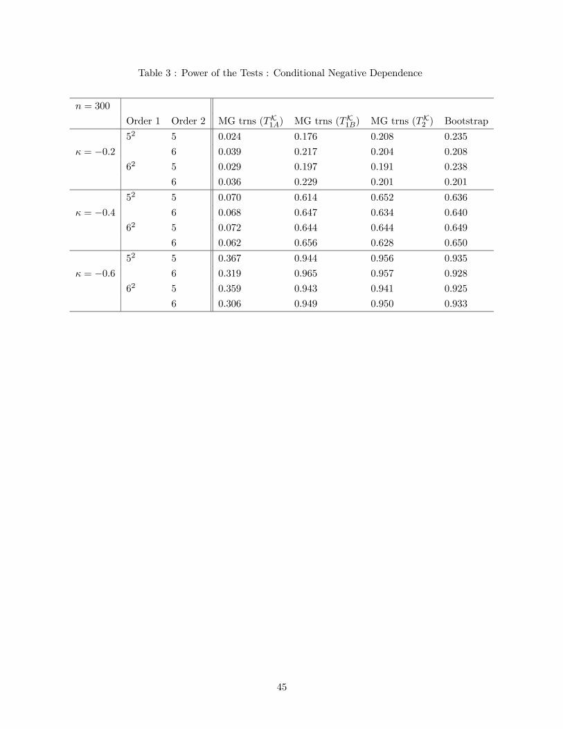
Table 3 : Power of the Tests : Conditional Negative Dependence

n = 300

Order 1 Order 2 MG trns (TK1A) MG trns (TK1B) MG trns (TK2 ) Bootstrap

52 5 0.024 0.176 0.208 0.235

κ = −0.2 6 0.039 0.217 0.204 0.208

62 5 0.029 0.197 0.191 0.238

6 0.036 0.229 0.201 0.201

52 5 0.070 0.614 0.652 0.636

κ = −0.4 6 0.068 0.647 0.634 0.640

62 5 0.072 0.644 0.644 0.649

6 0.062 0.656 0.628 0.650

52 5 0.367 0.944 0.956 0.935

κ = −0.6 6 0.319 0.965 0.957 0.928

62 5 0.359 0.943 0.941 0.925

6 0.306 0.949 0.950 0.933

45

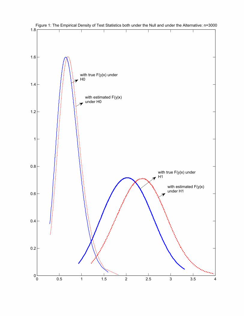
0 0.5 1 1.5 2 2.5 3 3.5 40

0.2

0.4

0.6

0.8

1

1.2

1.4

1.6

1.8Figure 1: The Empirical Density of Test Statistics both under the Null and under the Alternative: n=3000

with true F(y|x) underH0

with estimated F(y|x)under H0

with true F(y|x) underH1

with estimated F(y|x)under H1

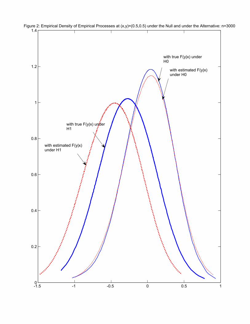
-1.5 -1 -0.5 0 0.5 10

0.2

0.4

0.6

0.8

1

1.2

1.4Figure 2: Empirical Density of Empirical Processes at (x,y)=(0.5,0.5) under the Null and under the Alternative: n=3000

with true F(y|x) underH0

with true F(y|x) underH1

with estimated F(y|x)under H0

with estimated F(y|x)under H1