Dimensions and spectral triples - uniroma2.itisola/research/preprints/GuIs10.pdf · there are λj...

Dimensions and spectral triples

for fractals in RN

Daniele Guido, Tommaso Isola

Dipartimento di Matematica, Universita di Roma “Tor Vergata”, I–00133 Roma,Italy. E-mail: [email protected], [email protected]

Abstract

Two spectral triples are introduced for a class of fractals in RN .

The definitions of noncommutative Hausdorff dimension and noncom-mutative tangential dimensions, as well as the corresponding Hausdorffand Hausdorff-Besicovitch functionals considered in [7], are studied forthe mentioned fractals endowed with these spectral triples, showing inmany cases their correspondence with classical objects. In particular, forany limit fractal, the Hausdorff-Besicovitch functionals do not depend onthe generalized limit ω.

0 Introduction.

In this paper we extend the analysis we made in [7] to fractals in RN , more pre-

cisely we define spectral triples for a class of fractals and compare the classicalmeasures, dimensions and metrics with the measures, dimensions and metricsobtained from the spectral triple, in the framework of A. Connes’ noncommu-tative geometry [2].

The class of fractals we consider is the class of limit fractals, namely fractalswhich can be defined as Hausdorff limits of sequences of compact sets obtainedvia sequences of contraction maps. This class contains the self-similar fractalsand is contained in the wider class of random fractals [12]. On any limit frac-tal, the described limit procedure produces also a family of limit measures µα,α > 0. Among limit fractals, we consider in particular the translation frac-tals, namely those for which the generating similarities of a given level have thesame similarity parameter. It turns out that for translation fractals all the limitmeasures µα coincide.

For limit fractals we introduce spectral triples which generalise the one con-sidered by Connes in [2] for Cantor-like fractals, namely are based on an ap-proximation of the fractal with sequences of pairs of points. In the first spectraltriple, the sequences consist of all descendants, via the generating similarities,

1

1 CLASSICAL ASPECTS 2

of one (or finitely many) ancestral pair. In the second triple, among the de-scendants of a single ancestor via the generating similarities, we consider allparent-child pairs.

In both cases, when translation fractals are considered, we prove that thenoncommutative Hausdorff dimension and tangential dimensions defined in [7]coincide with their classical counterparts computed in [9, 10]. Let us recallthat the noncommutative tangential dimensions are the extreme points of thetraceability interval, namely of the set of (singular) traceability exponents forthe inverse modulus of the Dirac operator. Therefore any of these exponentsgives rise to a singular trace τω which in turn defines a trace on the algebra A

of the spectral triple, hence, by Riesz theorem, a measure on the fractal. Fortranslation fractals all these measures coincide with the limit measure. In thecase of the parent-child triple, an analogous result holds for any limit fractal,i.e. the measure coming from the traceability exponent α coincides with thelimit measure µα. As a consequence, the measure generated by a singular traceτω is well defined, namely does not depend on the generalised limit procedureω.

Finally we study the distance on the fractal induced a la Connes by the spec-tral triple. In the case of the parent-child triple, the noncommutative distanceis always equivalent to the Euclidean distance, namely they induce the sametopology. Then we compare the noncommutative distance with the Euclideangeodesic distance, namely with the distance defined in terms of rectifiable curvescontained in the fractal (when they exist). We prove that the identity map fromthe fractal endowed with the geodesic distance to the fractal endowed with thenoncommutative distance is Lipschitz. As a consequence, when the Euclideandistance and the geodesic distance are bi-Lipschitz, this holds for the noncom-mutative distance too.

1 Classical aspects

We start this Section by recalling known results on self-similar fractals, then weintroduce the class of limit fractals and their limit measures, and give some ex-amples. We then introduce an open set condition which allows us to characterisethe limit measures on the fractal (Theorem 1.7), and to compute them in caseof translation limit fractals, under a mild assumption (Theorem 1.8). Finally,we recall the notions of tangential dimensions for metric spaces and measuresfrom [9, 10].

1.1 Preliminaries

The general reference for this Subsection is [4].Hausdorff measure and dimension. Let (X, ρ) be a metric space, andlet h : [0,∞) → [0,∞) be non-decreasing and right-continuous, with h(0) =0. When E ⊂ X , define, for any δ > 0, Hh

δ (E) := inf{∑∞

i=1 h(diamAi) :∪iAi ⊃ E, diamAi ≤ δ}. Then the Hausdorff-Besicovitch (outer) measure of E


is defined asH

h(E) := limδ→0

Hhδ (E).

If h(t) = tα, Hα is called Hausdorff (outer) measure of order α > 0.

The number

dH(E) := sup{α > 0 : Hα(E) = +∞} = inf{α > 0 : H

α(E) = 0}

is called Hausdorff dimension of E.Selfsimilar fractals. Let {wj}j=1,...,p be contracting similarities of R

N , i.e.there are λj ∈ (0, 1) such that ‖wj(x) − wj(y)‖ = λj‖x − y‖, x, y ∈ R

N .Denote by K(RN ) the family of all non-empty compact subsets of R

N , endowedwith the Hausdorff metric, which turns it into a complete metric space. ThenW : K ∈ K(RN ) → ∪p

j=1wj(K) ∈ K(RN ) is a contraction.

Definition 1.1. The unique non-empty compact subset F of RN such that

F = W (F ) =

p⋃

j=1

wj(F )

is called the self-similar fractal defined by {wj}j=1,...,p.

If we denote by ProbK(RN ) the set of probability measures on RN with com-

pact support endowed with the Hutchinson metric, i.e. d(µ, ν) := sup{|∫

fdµ−∫

fdν| : ‖f‖Lip ≤ 1}, then the map

T : ProbK(RN ) → ProbK(RN )µ 7→

∑pj=1 λs

jµ ◦ w−1j

is a contraction, where s > 0 is the unique real number, called similarity di-mension, satisfying

∑pj=1 λs

j = 1. We then observe that if µ has support K,then Tµ has support W (K). Since the sequence Wn(K) is convergent, it turnsout that it is bounded, namely there exists a compact set K0 containing thesupports of all the measures T nµ. But on the space Prob(K0) the Hutchinsonmetric induces the weak∗ topology, and this space is compact in such topology,hence complete in the Hutchinson metric. Therefore there exists a fixed pointof T in ProbK(RN ), which is of course unique.Open Set Condition. The similarities {wj}j=1,...,p are said to satisfy theopen set condition if there is a non-empty bounded open set V ⊂ R

N suchthat ∪p

j=1wj(V ) ⊂ V and wi(V ) ∩ wj(V ) = ∅, i 6= j. In this case dH(F ) = s,the similarity dimension, and the Hausdorff measure Hs is non-trivial on F .Therefore H

s|F is the unique (up to a constant factor) Borel measure µ, withcompact support, such that µ(A) =

∑pj=1 λs

jµ(w−1j (A)), for any Borel subset A

of RN .


1.2 Limit fractals.

Several generalisations of the class of self-similar fractals have been studied.Here we propose a new one, that we call the class of limit fractals. For itsconstruction we need the following theorem.

Theorem 1.2. Let (X, ρ) be a complete metric space, Tn : X → X be such thatthere are λn ∈ (0, 1) for which ρ(Tnx, Tny) ≤ λnρ(x, y), for x, y ∈ X. Assume∑∞

n=1

∏nj=1 λj < ∞, and there is x ∈ X such that supn∈N

ρ(Tnx, x) < ∞. Then

(i) supn∈N ρ(Tny, y) < ∞, for any y ∈ X,

(ii) limn→∞ T1 ◦ T2 ◦ · · · ◦ Tnx = x0 ∈ X for any x ∈ X.

Proof. (i) ρ(Tny, y) ≤ ρ(Tny, Tnx) + ρ(Tnx, x) + ρ(x, y) ≤ (1 + λn)ρ(x, y) +ρ(Tnx, x), so that supn∈N ρ(Tny, y) ≤ 2ρ(x, y) + supn∈N ρ(Tnx, x) < ∞.(ii) Set M := supn∈N

ρ(Tnx, x) < ∞, and Sn := T1 ◦ T2 ◦ · · · ◦ Tn, n ∈N. As ρ(Sn+1x, Snx) ≤ λ1λ2 · · ·λnρ(Tn+1x, x) ≤ Mλ1λ2 · · ·λn, there follows,for any p ∈ N, ρ(Sn+px, Snx) ≤ ρ(Sn+px, Sn+p−1x) + . . . + ρ(Sn+1x, Snx) ≤

M∑n+p−1

k=n

∏kj=1 λk ≤ M

∑∞k=n

∏kj=1 λk → 0, as n → ∞, that is {Snx} is

Cauchy in X . Therefore there is x0 ∈ X such that Snx → x0.Let us prove that x0 is independent of x. Indeed, if y ∈ X , then ρ(Snx, Sny) ≤λ1λ2 · · ·λnρ(x, y) → 0, as n → ∞, so that Snx and Sny have the same limit.

Remark 1.3. A sufficient condition for∑∞

n=1

∏nj=1 λj < ∞ to hold is

supn∈N

λn < 1.

We now describe the class of limit fractals. Let {wnj}, n ∈ N, j = 1, . . . , pn,be contracting similarities of R

N , with contraction parameter λnj ∈ (0, 1). Set,for any n ∈ N, Σn := {σ : {1, . . . , n} → N : σ(k) ∈ {1, . . . , pk}, k = 1, . . . , n},Σ := ∪n∈NΣn, Σ∞ := {σ : N → N : σ(k) ∈ {1, . . . , pk}, k ∈ N}, and writewσ := w1σ(1) ◦w2σ(2) ◦ · · · ◦wnσ(n), λσ := λ1σ(1)λ2σ(2) · · ·λnσ(n), for any σ ∈ Σn.

Assume λ := supn,j λnj < 1 and {wσ(x) : σ ∈ Σ} is bounded, for some (hence

any) x ∈ RN . Then, by Theorem 1.2, the sequence of maps Wn : K ∈ K(RN ) →

∪pn

j=1wnj(K) ∈ K(RN ) is such that {W1◦W2◦· · ·◦Wn(K)} has a limit in K(RN ),

which is independent of K ∈ K(RN ).

Definition 1.4. The unique compact set F which is the limit of {W1 ◦W2 ◦· · ·◦Wn(K)}n∈N is called the limit fractal defined by {wnj}. In the particular casethat λnj = λn, j = 1, . . . , pn, n ∈ N, F is called a translation (limit) fractal.

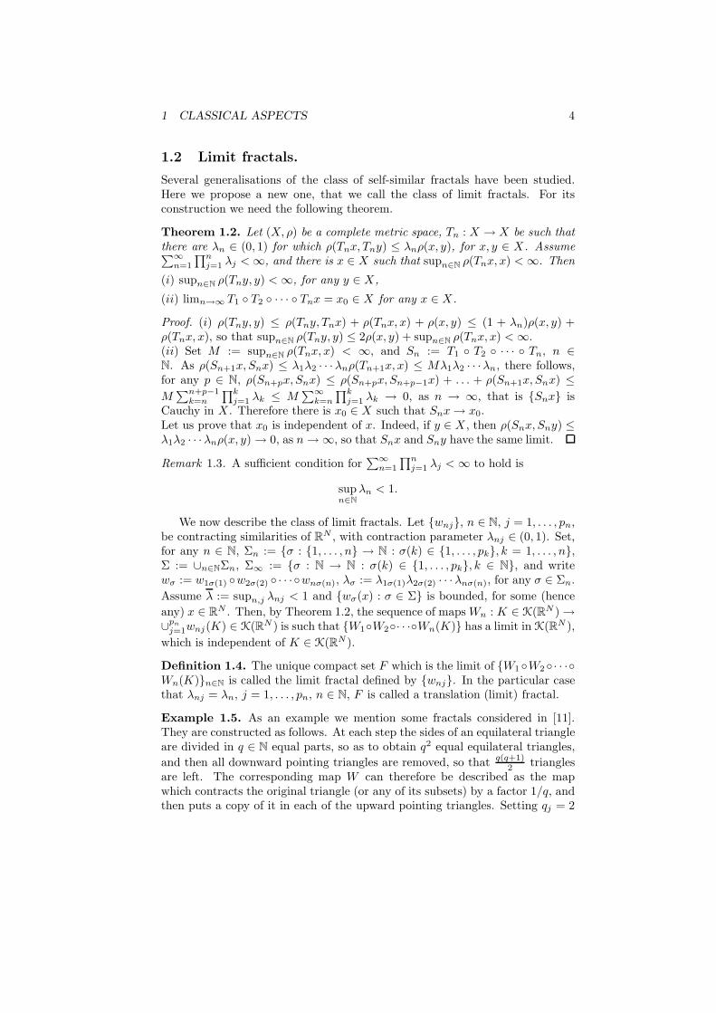
Example 1.5. As an example we mention some fractals considered in [11].They are constructed as follows. At each step the sides of an equilateral triangleare divided in q ∈ N equal parts, so as to obtain q2 equal equilateral triangles,

and then all downward pointing triangles are removed, so that q(q+1)2 triangles

are left. The corresponding map W can therefore be described as the mapwhich contracts the original triangle (or any of its subsets) by a factor 1/q, andthen puts a copy of it in each of the upward pointing triangles. Setting qj = 2


if (k − 1)(2k − 1) < j ≤ (2k − 1)k and qj = 3 if k(2k − 1) < j ≤ k(2k + 1),k = 1, 2, . . . , we get a translation fractal with dimensions given by (see Theorem1.14)

δ =log 3

log 2< d = d =

log 18

log 6< δ =

log 6

log 3,

where δ, δ, d, d denote the lower tangential, the upper tangential, the lower localand the upper local dimensions. The first four steps (q = 2, 3, 3, 2) of theprocedure above are shown in Figure 1.

Figure 1: Modified Sierpinski

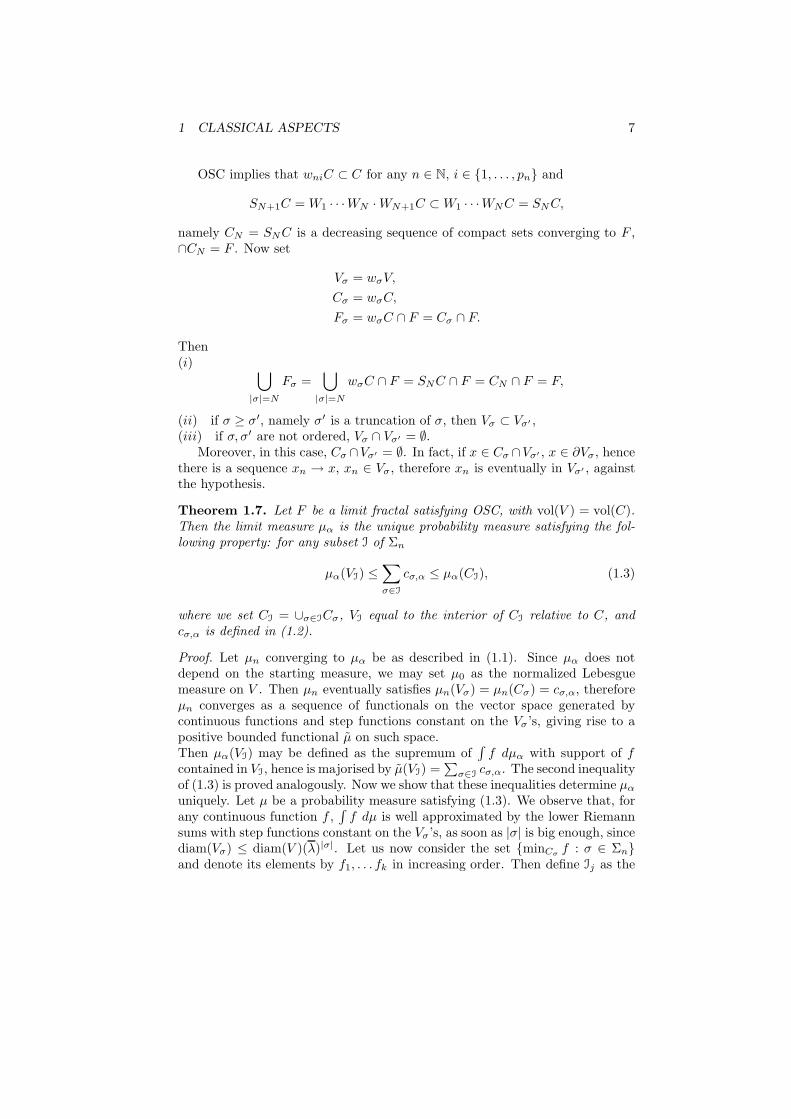
The procedure considered above can, of course, be applied also to othershapes. For example, at each step the sides of a square are divided in 2q + 1,q ∈ N, equal parts, so as to obtain (2q + 1)2 equal squares, and then 2q(q + 1)squares are removed, so that to remain with a chessboard. In particular, wemay set qj = 2 if k(2k + 1) < j ≤ (2k + 1)(k + 1) and qj = 1 if k(2k − 1) < j ≤k(2k + 1), k = 0, 1, 2, . . . , getting a translation fractal with dimensions given by(see Theorem 1.14)

δ =log 5

log 3< d = d =

log 65

log 15< δ =

log 13

log 5.

The first three steps (q = 1, 2, 1) of this procedure are shown in Figure 2.

As before, we may consider the action of the similarities on measures, besidesthat on sets. Given α > 0 we set

Tn : ProbK(RN ) → ProbK(RN )µ 7→ 1

Pp

j=1λα

nj

∑pj=1 λα

njµ ◦ w−1nj


Figure 2: Modified Vicsek

and consider the sequence {T1 ◦ T2 ◦ · · · ◦ Tnµ}n∈N. As before the supports ofall such measures are contained in a common compact set, therefore Theorem1.2 applies and we get a unique limit measure µα, depending on the chosen α.

As a consequence, if µ0 is a probability measure and α > 0, µn := T1 ◦ T2 ◦· · · ◦ Tnµ0 satisfies

µn(A) =∑

|σ|=n

cσ,αµ0(w−1σ (A)), (1.1)

where

cσ,α :=λα

σ∑

|σ′|=|σ| λασ′

. (1.2)

In particular, if F is a translation (limit) fractal,

cσ,α =1

p1p2 · · · p|σ|, ∀α > 0,

so that the limit measures µα all coincide, and will be denoted by µlim.

1.3 Hausdorff dimension and limit measures

Assumption 1.6. Open Set Condition: There is a bounded open set V suchthat wni(V ) ⊂ V for any n ∈ N, i ∈ {1, . . . , pn} and wn,iV ∩wn,jV = ∅ if i 6= j.We also assume that V is regular, namely the Lebesgue measure of V is equalto the Lebesgue measure of its closure C and V is equal to the interior of C.


OSC implies that wniC ⊂ C for any n ∈ N, i ∈ {1, . . . , pn} and

SN+1C = W1 · · ·WN · WN+1C ⊂ W1 · · ·WNC = SNC,

namely CN = SNC is a decreasing sequence of compact sets converging to F ,∩CN = F . Now set

Vσ = wσV,

Cσ = wσC,

Fσ = wσC ∩ F = Cσ ∩ F.

Then(i)

⋃

|σ|=N

Fσ =⋃

|σ|=N

wσC ∩ F = SNC ∩ F = CN ∩ F = F,

(ii) if σ ≥ σ′, namely σ′ is a truncation of σ, then Vσ ⊂ Vσ′ ,(iii) if σ, σ′ are not ordered, Vσ ∩ Vσ′ = ∅.

Moreover, in this case, Cσ ∩Vσ′ = ∅. In fact, if x ∈ Cσ ∩Vσ′ , x ∈ ∂Vσ, hencethere is a sequence xn → x, xn ∈ Vσ, therefore xn is eventually in Vσ′ , againstthe hypothesis.

Theorem 1.7. Let F be a limit fractal satisfying OSC, with vol(V ) = vol(C).Then the limit measure µα is the unique probability measure satisfying the fol-lowing property: for any subset I of Σn

µα(VI) ≤∑

σ∈I

cσ,α ≤ µα(CI), (1.3)

where we set CI = ∪σ∈ICσ, VI equal to the interior of CI relative to C, andcσ,α is defined in (1.2).

Proof. Let µn converging to µα be as described in (1.1). Since µα does notdepend on the starting measure, we may set µ0 as the normalized Lebesguemeasure on V . Then µn eventually satisfies µn(Vσ) = µn(Cσ) = cσ,α, thereforeµn converges as a sequence of functionals on the vector space generated bycontinuous functions and step functions constant on the Vσ’s, giving rise to apositive bounded functional µ on such space.Then µα(VI) may be defined as the supremum of

∫

f dµα with support of fcontained in VI, hence is majorised by µ(VI) =

∑

σ∈Icσ,α. The second inequality

of (1.3) is proved analogously. Now we show that these inequalities determine µα

uniquely. Let µ be a probability measure satisfying (1.3). We observe that, forany continuous function f ,

∫

f dµ is well approximated by the lower Riemannsums with step functions constant on the Vσ’s, as soon as |σ| is big enough, sincediam(Vσ) ≤ diam(V )(λ)|σ|. Let us now consider the set {minCσ

f : σ ∈ Σn}and denote its elements by f1, . . . fk in increasing order. Then define Ij as the


set of σ ∈ Σn such that minCσf ≥ fj , Cj as the union of the Cσ for σ ∈ Ij, Vj

as the interior of Cj . Then

f1 +

k∑

i=2

(fi − fi−1)µ(Vi) ≤ f1 +

k∑

i=2

(fi − fi−1)

(

∑

σ∈Ii

cσ,α

)

≤ f1 +

k∑

i=2

(fi − fi−1)µ(Ci) ≤

∫

f dµ.

The second term may be rewritten as

∑

σ∈Σn

minCσ

f cσα,

therefore∫

f dµ = limn→∞

∑

σ∈Σn

minCσ

f cσα,

hence there is only one probability measure satisfying (1.3).

Let now F be a translation fractal (λn,i independent of i), and, to avoid triv-iality, assume pn ≥ 2 for any n ∈ N. The OSC condition implies vol(Sn−1C) =∑pn

i=1 vol(wniSn−1C) = pnλNn vol(Sn−1C), so that 2λN

n ≤ 1, i.e. λn ≤ 2−1/N .We set

Λn =

n∏

i=1

λi, Pn =

n∏

i=1

pi. (1.4)

Theorem 1.8. Let F be a translation fractal, with the notation above, andassume p := supn pn < ∞. Then

dH(F ) = lim infn→∞

log Pn

log 1/Λn.

Moreover the Hausdorff measure corresponding to d := dH(F ) is non trivial ifand only if lim inf(log Pn − d log 1/Λn) is finite.

Proof. Let us consider the family P of finite coverings of F , the subfamily P(Σ)of coverings made from sets of {Cσ : σ ∈ Σ}, and the subfamily P

′(Σ), whosecoverings consist of Cσ, σ ∈ Σ, |σ| = const. If P ∈ P, |P | denotes the maximumdiameter of the sets in P . Clearly, for any α > 0, we have

Hα(F ) = limε→0

inf|P |≤εP∈P

∑

E∈P

(diamE)α ≤ limε→0

inf|P |≤ε

P∈P(Σ)

∑

E∈P

(diamE)α

≤ limε→0

inf|P |≤ε

P∈P′(Σ)

∑

E∈P

(diamE)α.


We shall show that the last two terms are indeed equal, and that the secondterm is majorised by a constant times the first, from which we derive

Hα(F ) ≍ lim infn→∞

PnΛαn,

hence the required equality and the last statement.We may assume without restriction that the diameter of V is equal to one.

Then set a := vol(V )vol(B(0,2)) , where vol denotes the Lebesgue measure. Then the

number of disjoint copies of V intersecting a ball of radius 1 is not greater thanthe number of disjoint copies of V contained in a ball of radius 2 which is inturn lower equal than a−1.

As a consequence, for any x ∈ F ,

#{σ ∈ Σn : Cσ ∩ BF (x, Λn) 6= ∅} ≤ a−1. (1.5)

For any ε > 0, let P =⋃n

i=1 Ei ∈ P, diamEi = ri ≤ ε. Let now xi ∈ Ei,Λni+1 ≤ ri ≤ Λni

.Since the set Ini

⊂ Σ of multi-indices of length ni such that⋃

σ∈IniCσ ⊃

B(xi, Λni) has cardinality majorised by a−1, and any such Cσ contains at most

p elements Cσ′ , with |σ′| = ni + 1, then the set of multi-indices Ini+1 ⊂ Σ oflength ni +1 such that

⋃

σ∈Ini+1Cσ ⊃ BF (xi, Λni

) has cardinality majorised by

p/a. Thereforen⋃

i=1

⋃

σ∈Ini+1

Cσ

is a covering of F of diameter less than ε and

n∑

i=1

∑

σ∈Ini+1

(diamCσ)α ≤n∑

i=1

p

aΛα

ni+1 ≤p

a

n∑

i=1

rαi . (1.6)

As a consequence

limε→0

inf|P |≤ε

P∈P(Σ)

∑

E∈P

(diamE)α ≤p

alimε→0

inf|P |≤ε

∑

E∈P

(diamE)α =p

aH

α(F ).

Now, for any n1 ≤ n0, let P be the optimal covering of F made of Cσ’s, withn1 ≤ |σ| ≤ n0, namely minimizing

∑

σ∈P (diamCσ)α, and choose Cσ0∈ P with

|σ0| = n0. This means that there is a Cσ, |σ| = n0 − 1, which is optimallycovered by some Cσ′ ’s of diameter Λn0

. Therefore this should be true for allother σ of length n0, namely the optimal covering is made of Cσ’s of the samesize. This shows the equality

limε→0

inf|P |≤ε

P∈P(Σ)

∑

E∈P

(diamE)α = limε→0

inf|P |≤ε

P∈P′(Σ)

∑

E∈P

(diamE)α

hence concludes the proof.


Remark 1.9. Let F be a translation fractal, with the notation above, and assumep := supn pn < ∞. Let G ⊂ F be closed. Then, with P(Σ) denoting the familyof finite coverings of G made from sets in {Vσ : σ ∈ Σ}, for any α > 0

Hα(G) ≍ lim

ε→0inf

|P |≤εP∈P(Σ)

∑

E∈P

(diamE)α.

It is clear that if the Fσ’s with σ ∈ Σn are essentially disjoint w.r.t. µα, thenµα(Fσ) = cσ,α. Now we will discuss some conditions implying the vanishing ofµα on the intersections of the Fσ’s.

Theorem 1.10. Let F be a translation fractal for which p := supn pn < ∞, Ga closed subset of F s.t. dH(G) < dH(F ). Then, µlim(G) = 0.As a consequence, if dH(wniC ∩ wnjC ∩ F ) < dH(F ), for any n, i 6= j, thenµlim(Fσ) = 1

P|σ|.

Proof. Let α be s.t. dH(G) < α < dH(F ), and ε > 0. Then, from Theorem 1.8and the Remark following it, there is n0 ∈ N, s.t. PnΛα

n ≥ 1, for all n ≥ n0,and there is I ⊂ Σ s.t. |σ| ≥ n0, for all σ ∈ I, and

∑

σ∈IΛα

σ ≤ ε, and G iscontained in the interior of ∪σ∈IFσ. By Urysohn’s lemma, there is f ∈ C(F ),0 ≤ f ≤ 1, f(x) = 1, x ∈ G, supp f ⊂ ∪σ∈IFσ. Then, with µk as in (1.1), andµ0 the normalised Lebesgue measure,

µlim(G) ≤

∫

f dµ = limk→∞

∫

f dµk ≤ limk→∞

µk(∪σ∈IFσ)

≤ limk→∞

∑

σ∈I

µk(Fσ) =∑

σ∈I

1

P|σ|=∑

σ∈I

1

P|σ|Λα|σ|

Λα|σ|

≤∑

σ∈I

Λα|σ| ≤ ε.

The thesis follows.

1.4 Tangential dimensions

Let (X, d) be a metric space, E ⊂ X . Let us denote by n(r, E) ≡ nr(E), resp.n(r, E) ≡ nr(E), the minimum number of open, resp. closed, balls of radius rnecessary to cover E, and by ν(r, E) ≡ νr(E) the maximum number of disjointopen balls of E of radius r contained in E.

Definition 1.11. [9] Let (X, d) be a metric space, E ⊂ X , x ∈ E. We callupper, resp. lower tangential dimension of E at x the (possibly infinite) numbers

δE(x) := lim infλ→0

lim infr→0

log n(λr, E ∩ B(x, r))

log 1/λ,

δE(x) := lim supλ→0

lim supr→0

log n(λr, E ∩ B(x, r))

log 1/λ.

2 NONCOMMUTATIVE ASPECTS 11

Tangential dimensions are invariant under bi-Lipschitz maps, and satisfyproperties which are characteristic of a dimension function.

Let µ be a locally finite Borel measure, namely µ is finite on bounded sets.Let us recall that the local dimensions of a measure at x are defined as

dµ(x) = lim infr→0

log µ(B(x, r))

log r,

dµ(x) = lim supr→0

log µ(B(x, r))

log r.

Now we introduce tangential dimensions for µ.

Definition 1.12. [10] The lower and upper tangential dimensions of µ aredefined as

δµ(x) := lim infλ→0

lim infr→0

log(

µ(B(x,r))µ(B(x,λr))

)

log 1/λ∈ [0,∞],

δµ(x) := lim supλ→0

lim supr→0

log(

µ(B(x,r))µ(B(x,λr))

)

log 1/λ∈ [0,∞].

Theorem 1.13. [10] Let µ be a locally finite Borel measure on X. Then thefollowing holds.

δµ(x) ≤ dµ(x) ≤ dµ(x) ≤ δµ(x).

Tangential dimensions are invariant under bi-Lipschitz maps.

Theorem 1.14. [10] Let F be a translation fractal with the notations above,µ = µlim, and assume p := supn pn < ∞. Then

dµ(x) = dH(F ) = lim infn→∞

log Pn

log 1/Λn,

dµ(x) = lim supn→∞

log Pn

log 1/Λn,

δF (x) = δµ(x) = lim infn,k→∞

log Pn+k − log Pn

log 1/Λn+k − log 1/Λn,

δF (x) = δµ(x) = lim supn,k→∞

log Pn+k − log Pn

log 1/Λn+k − log 1/Λn.

2 Noncommutative aspects

2.1 Singular traces on the compact operators of a Hilbert

space.

In this section we recall the theory of singular traces on B(H) as it was developedby Dixmier [3], who first showed their existence, and then in [13], [1] and [5].


A singular trace on B(H) is a tracial weight vanishing on the finite rankprojections. Any tracial weight is finite on an ideal contained in K(H) and maybe decomposed as a sum of a singular trace and a multiple of the normal trace.Therefore the study of (non-normal) traces on B(H) is the same as the study ofsingular traces. Moreover, making use of unitary invariance, a singular trace ofa given operator should depend only on its eigenvalue asymptotics, namely, if Aand B are positive compact operators on H and µn(A) = µn(B)+o(µn(B)), µn

denoting the n-th eigenvalue, then τ(A) = τ(B) for any singular trace τ . Themain problem about singular traces is therefore to detect which asymptoticsmay be “resummed” by a suitable singular trace, that is to say, which operatorsare singularly traceable.

In order to state the most general result in this respect we need some nota-tion. Let A be a compact operator. Then we denote by {µn(A)} the sequence ofthe eigenvalues of |A|, arranged in non-increasing order and counted with mul-tiplicity. We consider also the (integral) sequence {Sn(A)} defined as follows:

Sn(A) =

{

S↑n(A) :=

∑nk=1 µk(A) A /∈ L

1

S↓n(A) :=

∑∞k=n+1 µk(A) A ∈ L1,

where L1 denotes the ideal of trace-class operators. We call a compact operatorsingularly traceable if there exists a singular trace which is finite non-zero on |A|.We observe that the domain of such singular trace should necessarily containthe ideal I(A) generated by A. A compact operator is called eccentric if

S2nk(A)

Snk(A)

→ 1 (2.1)

for a suitable subsequence nk. Then the following theorem holds.

Theorem 2.1. [1] A positive compact operator A is singularly traceable iff it iseccentric. In this case there exists a sequence nk such that both condition (2.1)is satisfied and, for any generalised limit Limω on ℓ∞, the positive functional

τω(B) =

{

Limω

({

Snk(B)

Snk(A)

})

B ∈ I(A)+

+∞ B 6∈ I(A), B > 0,

is a singular trace whose domain is the ideal I(A) generated by A.

The best known eigenvalue asymptotics giving rise to a singular trace isµn ∼ 1

n , which implies Sn ∼ log n. The corresponding logarithmic singulartrace is generally called Dixmier trace.

Definition 2.2. [7] If A is a compact operator, set f(t) = − logµA(et), t ∈ R,where µA is the extension of µn(A) to a piecewise constant right continuous


function on [0,∞). Then define

δ(A) :=

limk→∞

lim supn→∞

log µn(A)µkn(A)

log k

−1

=

(

limh→∞

lim supt→∞

f(t + h) − f(t)

h

)−1

δ(A) :=

limk→∞

lim infn→∞

log µn(A)µkn(A)

log k

−1

=

(

limh→∞

lim inft→∞

f(t + h) − f(t)

h

)−1

d(A) :=

(

lim infn→∞

log µn(A)

log 1/n

)−1

=

(

lim inft→∞

f(t)

t

)−1

.

Moreover, we say that α > 0 is an exponent of singular traceability for A if |A|α

is singularly traceable.

Theorem 2.3. [7] Let A be a compact operator. Then, the set of singular trace-ability exponents of A is the relatively closed interval in (0,∞) whose endpointsare δ(A) and δ(A). In particular, if d(A) is finite nonzero, it is an exponent ofsingular traceability.

Note that the interval of singular traceability may be (0,∞), as shown in [6].In [8] the previous Theorem has been generalised to any semifinite factor, andsome questions concerning the domain of a singular trace have been considered.

2.2 Singular traces and spectral triples

In this section we shall discuss some notions of dimension in noncommutativegeometry in the spirit of Hausdorff-Besicovitch theory.

As is known, the measure for a noncommutative manifold is defined via asingular trace applied to a suitable power of some geometric operator (e.g. theDirac operator of the spectral triple of Alain Connes). Connes showed that suchprocedure recovers the usual volume in the case of compact Riemannian mani-folds, and more generally the Hausdorff measure in some interesting examples[2], Section IV.3.

Let us recall that (A, H, D) is called a spectral triple when A is an algebraacting on the Hilbert space H, D is a self adjoint operator on the same Hilbertspace such that [D, a] is bounded for any a ∈ A, and D has compact resolvent.In the following we shall assume that 0 is not an eigenvalue of D, the generalcase being recovered by replacing D with D|ker(D)⊥ . Such a triple is called d+-

summable, d ∈ (0,∞), when |D|−d belongs to the Macaev ideal L1,∞ = {a :S↑

n(a)log n < ∞}.

The noncommutative version of the integral on functions is given by theformula Trω(a|D|−d), where Trω is the Dixmier trace, i.e. a singular tracesumming logarithmic divergences. By the arguments below, such integral canbe non-trivial only if d is the Hausdorff dimension of the spectral triple, but eventhis choice does not guarantee non-triviality. However, if d is finite non-zero,we may always find a singular trace giving rise to a non-trivial integral.


Theorem 2.4. [7] Let (A, H, D) be a spectral triple. If s is an exponent ofsingular traceability for |D|−1, namely there is a singular trace τ which is non-trivial on the ideal generated by |D|−s, then the functional a 7→ τ(a|D|−s) is atrace state (Hausdorff-Besicovitch functional) on the algebra A.

Remark 2.5. When (A, H, D) is associated to an n-dimensional compact mani-fold M , or to the fractal sets considered in [2], the singular trace is the Dixmiertrace, and the associated functional corresponds to the Hausdorff measure. Thisfact, together with the previous theorem, motivates the following definition.

Definition 2.6. [7] Let (A, H, D) be a spectral triple, Trω the Dixmier trace.

(i) We call α-dimensional Hausdorff functional the map a 7→ Trω(a|D|−α);

(ii) we call (Hausdorff) dimension of the spectral triple the number

d(A, H, D) = inf{d > 0 : |D|−d ∈ L1,∞0 } = sup{d > 0 : |D|−d 6∈ L

1,∞},

where L1,∞0 = {a :

S↑n(a)

log n → 0}.

(iii) we call minimal, resp. maximal dimension of the spectral triple the quantityδ(|D|−1), resp. δ(|D|−1), hence |D|α is singularly traceable iff α ∈ [δ, δ] ∩(0, +∞).

(iv) For any s between the minimal and the maximal dimension, we call thecorresponding trace state on the algebra A a Hausdorff-Besicovitch functionalon (A, H, D).

Theorem 2.7. [7]

(i) d(A, H, D) = d(|D|−1).

(ii) d := d(A, H, D) is the unique exponent, if any, such that the d-dimensionalHausdorff functional is non-trivial.

(iii) If d ∈ (0,∞), it is an exponent of singular traceability.

Let us observe that a singular trace, hence in particular the α-dimensionalHausdorff functional, depends on a generalized limit procedure ω, however itsvalue is uniquely determined on the operators a ∈ A such that a|D|−d is mea-surable in the sense of Connes [2]. By an abuse of language we call measurablesuch operators.

As in the commutative case, the dimension is the supremum of the α’ssuch that the α-dimensional Hausdorff measure is everywhere infinite and theinfimum of the α’s such that the α-dimensional Hausdorff measure is identicallyzero. Concerning the non-triviality of the d-dimensional Hausdorff functional,we have the same situation as in the classical case. Indeed, according to theprevious result, a non-trivial Hausdorff functional is unique (on measurableoperators) but does not necessarily exist. In fact, if the eigenvalue asymptoticsof D is e.g. n log n, the Hausdorff dimension is one, but the 1-dimensionalHausdorff measure gives the null functional.


However, if we consider all singular traces, not only the logarithmic ones,and the corresponding trace functionals on A, as we said, there exists a nontrivial trace functional associated with d(A, H, D) ∈ (0,∞), but d(A, H, D) isnot characterized by this property. In fact this is true if and only if the minimaland the maximal dimension coincide. A sufficient condition is the following.

Proposition 2.8. [7] Let (A, H, D) be a spectral triple with finite non-zero

dimension d. If there exists lim µn(D−1)µ2n(D−1) ∈ (1,∞), d is the unique exponent of

singular traceability of D−1.

2.3 A spectral triple for fractals

In this Subsection we introduce a spectral triple on limit fractals, by extendingan idea of Connes for Cantor-like fractals. We compute its various dimensions,and recognise the noncommutative Hausdorff functional as the one arising fromthe limit measure on the fractal. Little can we say on the metric defined by thisspectral triple, so in the next Subsection we propose a different spectral triple.

Let F be a limit fractal which satisfies OSC (se Assumption 1.6) with respectto the open set V , and let C be the closure of V . Choose two points x, y ∈ C,and denote with r their distance. Also, construct the sequences xσ = wσx,yσ = wσy, σ ∈ Σ and note that

‖xσ − yσ‖ = rσ := rλσ .

Then let H be the ℓ2 space on the points xσ, yσ, and consider the naturalrepresentation of the Borel functions on C as multiplication operators on theelements of H. Then let

D :=⊕

σ∈Σ

1

‖xσ − yσ‖

(

0 11 0

)

Now we consider the spectral triple (A, H, D) where H and D are definedas above, and A is the algebra of continuous functions on C such that [D, f ] isbounded.

Remark 2.9. We may generalise the construction of the spectral triple by consid-ering a finite number of ancestral pairs {xi, yi}, e.g., for a Sierpinski like fractalas in Figure 1, the pairs of extreme points of the three sides of the originaltriangle.

Theorem 2.10. Let F be a limit fractal, (A, H, D) the spectral triple de-scribed above, α a singular traceability exponent for |D|−1. Then the Hausdorff-Besicovitch functional coincides, via Riesz Theorem, with the limit measure µα.

Proof. Let us first assume that the ancestral pair {x, y} is contained in V . Thenthe proof can be done as in Proposition 2.15 and Theorem 2.16.

Now take a generic pair {x′, y′}, with ‖x′ − y′‖ = r′, and the correspond-ing spectral triple (A, H, D′), where the Hilbert spaces are naturally identi-fied. While the family of eigenvalues (with multiplicity) of |D|−1 is given by


{rλσ : σ ∈ Σ}, each with multiplicity 2, the family of eigenvalues (with multi-plicity) of |D′|−1 is given by {r′λσ : σ ∈ Σ}, each with multiplicity 2. Thereforethe spectral triples have the same set of traceability exponents, and if α is oneof them, τ is a singular trace such that τ(|D|−α) = 1, then τ ′(|D′|−α) = 1, withτ ′ =

(

rr′

)ατ .

Now let f be a Lipschitz function on C, with Lipschitz constant L. f |D|−α

is a multiplication operator, with eigenvalues (with multiplicity)

{rαλασf(xσ), rαλα

σf(yσ) : σ ∈ Σ}.

Then

f |D′|−α =

(

r′

r

)α

f |D|−α + R,

where R is a selfadjoint operator with eigenvalues (with multiplicity)

{(r′)αλασ(f(x′

σ) − f(xσ)), (r′)αλασ(f(y′

σ) − f(yσ)) : σ ∈ Σ}.

Since |f(x′σ) − f(xσ)| ≤ L‖x′

σ − xσ‖ = Lλσ‖x′ − x‖, the operator |R| can bemajorised by a positive operator S with eigenvalues {LM(r′)αλα+1

σ : σ ∈ Σ},each with multiplicity 2, where M = max(‖x′ − x‖, ‖y′ − y‖). Clearly theoperator S is infinitesimal w.r.t. |D|−α, hence

τ ′(f |D′|−α) =

(

r′

r

)α

τ ′(f |D|−α) + τ ′(R) = τ(f |D|−α) =

∫

f dµα.

Since Lipschitz functions are dense, we get the thesis.

Remark 2.11. (i) When F is a translation fractal, and the Hausdorff dimensionof the sets Fσ∩Fσ′ is strictly lower than the Hausdorff dimension of F , |σ| = |σ′|,then Theorem 1.10 applies, giving

µlim(Fσ) = P−1|σ| .

(i) Let us observe that for self-similar fractals, there is only one exponent ofsingular traceability, namely the similarity dimension s, and the correspondinglimit measure coincides with Hs.

Theorem 2.12. Let (A, D, H) be the spectral triple associated with a translationfractal F where the similarities wn,i, i = 1, . . . , pn have scaling parameter λn.Then the Hausdorff dimension is given by the formula

d = lim supn

∑n1 log pk

∑n1 log 1/λk

.

Proof. The eigenvalues of |D|−1 are given by r with multiplicity 2, rλ1 withmultiplicity 2p1, rλ1λ2 with multiplicity 2p1p2, and so on. Therefore, with


p0 := 1, λ0 := 1, and Λn, Pn as in (1.4),

Tr(|D|−α) = 2rα∞∑

k=0

k∏

i=0

(pkλk)α

= 2rα∞∑

n=0

elog Pn−α log 1/Λn

= 2rα∞∑

n=0

exp

(

log Pn

(

1 − αlog 1/Λn

log Pn

))

.

Denote by d :=(

lim infn→∞log 1/Λn

log Pn

)−1

. Then, if α > d, we get

lim infn→∞

αlog 1/Λn

log Pn=

α

d> 1

which implies that, for any sufficiently small ε > 0 there is nε ∈ N such that,for all n > nε,

1 − αlog 1/Λn

log Pn< −ε.

Since P−εn ≤ 2−nε, the series converges. Whereas, if α < d, as there is a

subsequence {nk} such thatlog 1/Λnk

log Pnk

→ d−1, we get

1 − αlog 1/Λnk

log Pnk

→ 1 −α

d> 0

and the series diverges. Therefore d(A, D, H) = d.

Theorem 2.13. Let (A, H, D) be the spectral triple associated with a translationfractal F , where the similarities wn,i, i = 1, . . . , pn have scaling parameter λn.Then

δ(A, H, D) = lim infn,k

∑n+kj=n log pj

∑n+kj=n log 1/λj

,

δ(A, H, D) = lim supn,k

∑n+kj=n log pj

∑n+kj=n log 1/λj

.

Proof. The eigenvalues of |D|−1 are the numbers rΛk, each with multiplicity2Pk. Therefore, the quantity 1

h (log 1/µ(et+h) − log 1/µ(et)), may be rewrittenas

log 1/Λk − log 1/Λm

log(

∑kj=0 Pj − ϑkPk

)

− log(

∑mj=0 Pj − ϑ′

mPm

) (2.2)

for suitable constants ϑk, ϑ′k in [0, 1).


Let us observe that, since pi ≥ 2,

log

k∑

j=0

Pj − ϑkPk

− log Pk ≤ log

∑kj=0 Pj

Pk

= log

k∑

j=0

k∏

i=j+1

1

pi

≤ log 2.

Since the denominator goes to infinity, additive perturbations of the numeratorand of the denominator by bounded sequences do not alter the lim sup, resp.lim inf, and the ratio above may be replaced by

log 1/Λk − log 1/Λm

log Pk − log Pm. (2.3)

Finally, since the denominator log Pk − log Pm goes to infinity if and only ifk − m → ∞, the thesis follows.

Remark 2.14. As in Connes’ book, we may introduce on F the metric definedby D, namely

d(x, y) := sup{|f(x) − f(y)| : f ∈ C(F ), ‖[D, f ]‖ ≤ 1}.

However it is not true, in general, that ι : (F, ‖·‖) → (F, d) is a homeomorphism.For example, let F be the Sierpinski gasket, x, y ∈ F being two vertices of theenveloping triangle. Then the metric d gives value +∞ to any pair of pointsin F sitting on a line which is not parallel to the side x, y. Nevertheless, ifwe consider three ancestral pairs for F as in remark 2.9, we get the Euclideangeodesic distance in F (cf. Theorem 2.23).

2.4 A different spectral triple

In this final Subsection we construct a spectral triple on a large subclass of limitfractals. We recognise the noncommutative Hausdorff functionals as the onesarising from the limit measures, and compare the “noncommutative metric” withthe Euclidean geodesic distance. In case of translation fractals, we compute thevarious dimensions associated to the spectral triple.

Let F be a limit fractal satisfying OSC (see Assumption 1.6). Let xni bethe fixed point of wni, and assume that the set W of all xni’s is not dense in V .Fix x∅ ∈ V \ W , then there is c > 0 s.t. ‖x∅ − xni‖ ≥ c, for all n, i, and

diam(C) ≥ ‖x∅ − wnix∅‖ ≥∣

∣

∣‖x∅ − xni‖ − ‖xni − wnix∅‖

∣

∣

∣

= (1 − λni)‖x∅ − xni‖ ≥ (1 − λ)c. (2.4)

Set xσ := wσx∅, and define

D :=⊕

σ∈Σ

p|σ|+1⊕

i=1

1

‖xσ − xσ·i‖

(

0 11 0

)


acting on

H =⊕

σ∈Σ

p|σ|+1⊕

i=1

ℓ2{xσ, xσ·i}

In the following we shall consider the spectral triple (A, H, D) with H andD defined as above, and A consisting of continuous functions f on C, acting onH as

(fξ)σ,i(xσ) = f(xσ)ξσ,i(xσ)

(fξ)σ,i(xσ·i) = f(xσ·i)ξσ,i(xσ·i),

and for which [D, f ] is bounded.

2.4.1 Measures and dimensions

For α > 0, a singular traceability exponent of |D|−1, set

∫

fdµ0α := τ(f |D|−α)

for any Borel function f , where τ is a singular trace such that τ(|D|−α) = 1.

Proposition 2.15. With the above notation, µ0α(Vσ) = µ0

α(Cσ) = cσ,α, for anyσ ∈ Σ.

Proof. Let σ, σ′ ∈ Σn, then

‖xσ·ρ − xσ·ρ·i‖ = ‖wσ·ρx∅ − wσ·ρ·ix∅‖ = λσ‖w−1σ wσ·ρx∅ − w−1

σ wσ·ρ·ix∅‖.

As w−1σ wσ·ρ is independent of σ, the operators λ−α

σ χVσ|D|−α and λ−α

σ′ χVσ′ |D|−α

have the same eigenvalues (with multiplicity) up to finitely many. Therefore,

1 = τ(|D|−α) =∑

σ′∈Σn

τ(χVσ′ |D|−α) =∑

σ′∈Σn

λασ′

λασ

τ(χVσ|D|−α),

so that µ0α(Vσ) = τ(χVσ

|D|−α) = cσ,α. Since∑

σ∈Σncσ,α = 1, we get µ0

α(Cσ) =cσ,α.

The set function µ0α is not σ-additive, however its restriction to continuous

functions gives rise to the Hausdorff-Besicovitch functional on C(F ) = A. Thefollowing holds:

Theorem 2.16. Let α be a traceability exponent. Then the measure associatedwith the Hausdorff-Besicovitch functional via the Riesz Theorem, coincides withthe limit measure µα. In particular it does not depend either on x∅ or on thegeneralised limit.


Proof. Let us show that the regularization µα of µ0α satisfies the inequalities

(1.3). Indeed

µα(VI) ≤ µ0α(VI) ≤

∑

σ∈I

µ0α(Cσ) =

∑

σ∈I

cσ,α.

Moreover,

µα(CI) ≥ µ0α(CI) ≥

∑

σ∈I

µ0α(Vσ) =

∑

σ∈I

cσ,α.

Then, by the uniqueness proved in Theorem 1.7, µα coincides with µα.

Theorem 2.17. Let (A, D, H) be the spectral triple associated with a translationfractal F , where the similarities wn,i, i = 1, . . . , pn have scaling parameter λn,and supn pn < +∞. Then

d(A, H, D) = lim supn

∑n1 log pk

∑n1 log 1/λk

δ(A, H, D) = lim infn,k

∑n+kj=n log pj

∑n+kj=n log 1/λj

,

δ(A, H, D) = lim supn,k

∑n+kj=n log pj

∑n+kj=n log 1/λj

.

Proof. The eigenvalues of |D|−1 are the numbers Λk,i := Λk‖x∅ − wk+1,ix∅‖,each with multiplicity 2Pk. It follows from (2.4) that there are 0 < c1 < c2 s.t.c1Λk ≤ Λk,i ≤ c2Λk, for all k ∈ N. Therefore

Tr(|D|−α) =∑

k∈N

Pk

pk+1∑

i=1

Λα

k,i ≍∑

k

PkΛαk ,

and the first equality follows as in Theorem 2.12. As for the others, the samecomputation in the proof of Theorem 2.13 can be performed.

From Theorems 1.14, 2.17 we get

Corollary 2.18. Let F be a translation (limit) fractal, µ its limit measure,(A, H, D) its associated spectral triple. Then, for any x ∈ F ,

d(A, H, D) = dµ(x),

δ(A, H, D) = δµ(x),

δ(A, H, D) = δµ(x).

2.4.2 Metrics

Let us now introduce on F the metric defined by D as in Connes’ book, namely

d(x, y) := sup{|f(x) − f(y)| : f ∈ C(C), ‖[D, f ]‖ ≤ 1}.


Lemma 2.19. ‖x − y‖ ≤ d(x, y), for all x, y ∈ F .

Proof. Let f be a Lipschitz function on C with Lipschitz constant ≤ 1. Then‖[D, f ]‖ ≤ 1, therefore ‖x − y‖ ≤ d(x, y).

Let us observe first that this distance and the Euclidean distance induce thesame topology.

Lemma 2.20. (i) Let σ ∈ Σn, x ∈ Fσ. Then d(x, xσ) ≤ diam(C)

1−λλσ.

(ii) Let σ, σ′ ∈ Σn be s.t. Fσ ∩ Fσ′ 6= ∅. Then d(xσ , xσ′) ≤ diam(C)

1−λ(λσ + λσ′).

Proof. (i). There is ρ ∈ Σ∞ s.t. x = xρ and the n-th truncation ρn of ρ is equalto σ, i.e., ρn(i) = σ(i), i = 1, . . . , n. Then

d(x, xσ) ≤∞∑

k=|σ|

d(xρk , xρk+1)

≤∞∑

k=|σ|

λρk diam(C) ≤diam(C)

1 − λλσ.

(ii) Let x ∈ Fσ ∩ Fσ′ . Then d(xσ, xσ′ ) ≤ d(x, xσ) + d(x, xσ′ ) ≤ diam(C)

1−λ(λσ +

λσ′).

Theorem 2.21. Let F be a limit fractal. Then ι : (F, ‖ · ‖) → (F, d) is ahomeomorphism.

Proof. Assume ι is discontinuous in x ∈ F , so that there are c > 0, {xn} ⊂ Fs.t. ‖xn − x‖ → 0, and d(xn, x) ≥ c, n ∈ N. From Lemma 2.20 we obtaink ∈ N s.t., for σ ∈ Σk, we have diam(Fσ) < c

2 . As ∪σ∈ΣkFσ = F , there is

σ ∈ Σk s.t. A := {n ∈ N : xn ∈ Fσ} is infinite, hence x ∈ Fσ. Thereforec ≤ d(xn, x) ≤ diam(Fσ) < c

2 , which is absurd.

The map ι is not bi-Lipschitz in general. This is true however when theEuclidean distance and the Euclidean geodesic distance in F are bi-Lipschitz.

Lemma 2.22. Let A ⊂ RN be a bounded open set, ρ ≥ 1. Then there are k ∈ N,

c > 0, such that, given similarities ϕ1, . . . , ϕk such that ϕi(A)∩ϕj(A) = ∅, i 6= j,with similarity parameters λ1 ≤ · · · ≤ λk satisfying λk ≤ ρλ1, and a rectifiablecurve γ such that γ ∩ ϕi(A) 6= ∅, ∀i = 1, . . . , k, we have ℓ(γ) > cλ1.

Proof. Possibly rescaling, it is not restrictive to assume that λ1 = 1. Let k ∈ N

be s.t. the infimum length of a rectifiable curve intersecting the closure ofk dilated copies of A with disjoint interior is 0. Then, for any n ∈ N, weget sequences of dilations ϕ1n, . . . , ϕkn such that ϕin(A) ∩ ϕjn(A) = ∅, and arectifiable curve γn with ℓ(γn) < 1

n such that γ ∩ ϕin(A) 6= ∅, i = 1, . . . , k,n ∈ N. Clearly it is not restrictive to assume that all curves γn start from thesame point x0, which implies that all the curves and copies of A are contained


in some compact set. By the assumptions above, all dilations lie in a compactset. Hence, possibly passing to a subsequence, we may assume that, for anyi = 1, . . . k, ϕin converges to a dilation ϕi of R

N and γn → γ in the Hausdorfftopology. Let us remark that in this way Ain → Ai in the Hausdorff topology,where Ai := ϕi(A), Ain := ϕin(A), i = 1, . . . , k, n ∈ N. As diam(γ) = 0, γconsists of a single point, indeed the point x0. Moreover γ ∩ Ai 6= ∅, for all i,i.e. x0 ∈ ∩k

i=1Ai.We claim that A1, . . . , Ak are disjoint. By contradiction, assume that Ai ∩ Aj

is not empty, namely that there exist points xi, xj ∈ A with ϕi(xi) = ϕj(xj),and let r > 0 be s.t. B(xi, r), B(xj , r) ⊂ A. Since the ϕi’s are dilations, thisimplies that B(ϕi(xi), r) ⊂ Ai, and the same for j. We have that ϕin(xi) andϕjn(xj) converge to the same point, hence, for a sufficiently large n, ‖ϕin(xi)−ϕjn(xj)‖ < r, so that Ain ∩ Ajn 6= ∅, which is absurd.Since x0 ∈ ∩k

i=1Ai, so that Ai ⊂ B(x0, ρ diam(A)), we obtain

ωNρN (diam(A))N = vol(B(x0, ρ diam(A))) ≥k∑

i=1

vol(Ai) ≥ k vol(A),

with ωN the volume of the unit ball in RN . Therefore, if we take the con-

stant k greater than ωN ρN (diam(A))N

vol(A) , the infimum length of a rectifiable curve

intersecting k dilated copies of A with disjoint interior cannot be 0.

Theorem 2.23. Let F be a limit fractal in RN , dgeo the Euclidean geodesic

distance in F , namely the distance defined in terms of rectifiable curves con-tained in the fractal (when they exist). Assume λ := infn,i λni > 0. Then thereis c ≥ 1 s.t. ‖x − y‖ ≤ d(x, y) ≤ cdgeo(x, y), x, y ∈ F .

Proof. The first inequality was proved above, let us prove the second. For anyε > 0, consider the set Σ(ε) consisting of the multi-indices σ such that λσ ≤ εbut λσn−1 > ε, where n = |σ| and σk denotes the k-th truncation of σ (asin the proof of Lemma 2.20). Then λσ = λn,σ(n)λσn−1 > λε. It is clear that∪σ∈Σ(ε)Fσ = F , and Vσ ∩ Vσ′ = ∅ if σ 6= σ′ are in Σ(ε).Now let x, y ∈ F , ε > 0. Choose a rectifiable curve γ in F connecting x andy, with ℓ(γ) < 2dgeo(x, y), and let σ1, . . . σk be the elements of Σ(ε) such thatCσi

∩ γ 6= ∅, ordered in such a way that x ∈ Cσ1, y ∈ Cσk

, and Cσi∩Cσi+1

6= ∅,i = 1, . . . , k − 1.By Lemma 2.20 we get

d(x, y) ≤ d(x, xσ1) +

k−1∑

i=1

d(xσi, xσi+1

) + d(xσk, y)

≤2 diam(C)

1 − λ

k∑

i=1

λσi≤

2 diam(C)kε

1 − λ.

Let us notice that k → ∞, when ε → 0.

REFERENCES 23

Now let kV ∈ N, cV > 0 be the constants associated to V and to 1/λ inLemma 2.22. Then

ℓ(γ) ≥ [k/kV ]cV λε

≥cV λ(1 − λ)

2 diam(C)

[k/kV ]

kd(x, y).

Passing to the limit for ε → 0, we get d(x, y) ≤ 4kV diam(C)

cV λ(1−λ)dgeo(x, y), i.e. the

thesis.

Remark 2.24. For many fractals, as Sierpinski gasket and carpet, Vicsek, Lind-strom snowflake etc., dgeo and the Euclidean distance are biLipschitz, hence alsod and the Euclidean distance are.

References

[1] S. Albeverio, D. Guido, A. Ponosov, S. Scarlatti. Singular traces and com-pact operators. J. Funct. Anal., 137 (1996), 281–302.

[2] A. Connes. Non Commutative Geometry. Academic Press, 1994.

[3] J. Dixmier. Existence de traces non normales. C.R. Acad. Sci. Paris, 262

(1966), 1107–1108.

[4] K. J. Falconer. The geometry of fractal sets. Cambridge University Press,1986.

[5] D. Guido, T. Isola. Singular traces and Novikov-Shubin invariants, in Oper-ator Theoretical Methods, Proceedings of the 17th Conference on OperatorTheory Timisoara (Romania) June 23-26, 1998, A. Gheondea, R.N. Golo-gan, D. Timotin Editors, The Theta Foundation, Bucharest 2000.

[6] D. Guido, T. Isola. Fractals in Noncommutative Geometry, in the Pro-ceedings of the Conference ”Mathematical Physics in Mathematics andPhysics”, Siena 2000, Edited by Roberto Longo, Fields Institute Commu-nications, Vol. 30 American Mathematical Society, Providence, RI, 2001

[7] D. Guido, T. Isola. Dimensions and singular traces for spectral triples, withapplications to fractals. Journ. Funct. Analysis, 203, (2003) 362-400

[8] D. Guido, T. Isola. On the domain of singular traces. Int. J. Math., 13

(2002), 667-674.

[9] D. Guido, T. Isola. Tangential dimensions I. Metric spaces. To appear inHouston J. Math., preprint math.FA/0305091.

[10] D. Guido, T. Isola. Tangential dimensions II. Measures. To appear in Hous-ton J. Math., preprint math.FA/0405174.

REFERENCES 24

[11] B. Hambly. Brownian motion on a homogeneous random fractal. Prob. Th.Rel. Fields, 94, (1992), 1-38.

[12] R.D. Mauldin, S.C. Williams. Random recursive constructions: asymptoticgeometric and topological properties. Trans. Amer. Math. Soc. 295 (1986),325–346.

[13] J.V. Varga. Traces on irregular ideals. Proc. A.M.S., 107 (1989), 715.

Dimensions and spectral triples - uniroma2.itisola/research/preprints/GuIs10.pdf · there are λj...

Documents

Transcript of Dimensions and spectral triples - uniroma2.itisola/research/preprints/GuIs10.pdf · there are λj...