Design, implementation and evaluation of an optimal ... · Design, implementation and evaluation of...

Design, implementation and evaluation of an optimal iterative learning

control algorithm

V. VITA A. VITAS G.E. CHATZARAKIS

Department of Electrical Engineering Educators

ASPETE-School of Pedagogical and Technological Education

Ν. Ηeraklion, 141 21 Athens

GREECE

[email protected]

Abstract: Iterative learning control (ILC) is used to control systems that operate in a repetitive mode, improving

tracking accuracy of the control by transferring data from one repetition of a task, to the next. In this paper an

optimal iterative learning algorithm for discrete linear systems is designed and implemented. The design and

implementation that have been done using Matlab® 7 and Simulink are described in detail. The algorithm is

applied on several representative discrete systems cases in order to be evaluated and to reveal its capabilities

and limitations.

Key-Words: Discrete linear systems; iterative learning control; Matlab® 7; simulation.

1 Introduction Iterative Learning Control (ILC) is a relatively new

concept in the control theory. It evolved from the

need to control dynamical systems that are supposed

to carry out a given task repetitively and more

specifically for systems where the desired output

values are a function of time and the task is carried

out repeatedly. A classical example is the robot in

the car industry that follows a given trajectory and

welds at specific points along the trajectory.

Normally the robot would be tuned once through

feedback or feedforward control or even a

combination of both. After the tuning, it would carry

out the repetitions performing in the same way. The

obvious drawback of this approach is the fact that if

there is an error between the measured trajectory

and the reference trajectory due to a wrong selection

of the control input trajectory, the robot will repeat

this error at each trial, i.e., if there is an error in the

performance it will repeat the same error at each

iteration.

To overcome this problem, Arimoto, one of the

inventors of ILC [1, 2], suggested that both the

information from the previous tasks or “trials” and

the current task should be used to improve the

control action during the current trial. In other

words, the controller should learn iteratively the

correct control actions in order to minimize the

difference between the output of the system and the

given reference signal. He called this method

“betterment process” [3]. This approach is more or

less an imitation of the learning process of every

intelligent being. Intelligent beings tend to learn by

performing a trial (i.e. selecting a control input) and

observing what was the end result of this control

input selection. After that they try to change their

behaviour (i.e. to pick up a new control input) in

order to get an improved performance during the

next trial. Based on the overall idea of ILC, the

procedure which results in a controller that learns

the correct control input and that learning is done

through iteration, the term Iterative Learning

Control is nowadays used to describe control

algorithms that result in the “betterment process” as

suggested by Arimoto [3]. In this work an optimal

iterative learning algorithm for discrete linear

systems is designed and implemented. The

algorithm is applied on several representative

discrete systems cases in order to be evaluated and

tested, producing very good and useful results.

2 Norm-optimal iterative learning

control algorithm The aim of the ILC algorithm [1, 5], is to find

iteratively an optimal input ∗u for the plant under

investigation. This input, when applied to the plant,

should generate an output ∗y that tracks the desired

output dy “as accurately as possible”. The use of

the phrase “as accurately as possible” states the

significance of obtaining the smallest possible

difference between the actual ∗y and desired dy

output. This difference is actually the error e and the

WSEAS TRANSACTIONS on CIRCUITS and SYSTEMS V. Vita, A. Vitas, G. E. Chatzarakis

ISSN: 1109-2734 39 Issue 2, Volume 10, February 2011

above lead to the conclusion that the error e is

desired to be minimal. The ultimate aim of the ILC

is to push the error e to zero. Thus it is clear that

applying an ILC algorithm will result in a two-

dimensional system because the information

propagates both along the time axis t and the

iteration axis k.

The two-dimensionality of the iterative learning

control introduces problems in the analysis as well

as the design of the system and hence the two-

dimensions are an expression of the systems

dependent dynamics: a) the trial index k and b) the

elapsed time t during each trial. In order to

overcome such difficulties an algorithm for Iterative

Learning Control is introduced, which has the

property of solving the two-dimensionality problem.

For the solution of this problem the cost function for

the system under investigation is introduced. The

minimization of the cost function will provide an

effective algorithm for iterative learning control

(ILC).

The following cost function is proposed [4]:

( ) 2

1

2

11 QkRkkk euuuJ +++ +−= (1)

where:

( )1+kuJ is the cost function with respect to the

current trial input, 2

1 kk uu −+ is the norm of the difference between the

current and previous trial inputs, 2

1+ke is the norm of the current error and

R, Q are symmetric and positive definite weighing

matrices. It is assumed that R and Q are diagonal

matrices, and for simplicity rIR = and qIQ = ,

where q and r are positive real numbers ( )ℜ∈rq, .

In ILC literature, researchers have suggested

different cost functions to solve the ILC problem.

The reasons that lead to the realization that the

selected cost function (1) is effective and

appropriate are the following: a) The 2

1 kk uu −+

factor represents the importance of keeping the

deviation of the input between the trials small.

Intuitively this should result in smooth convergence

behaviour. This requirement could also be stated as

the need for producing smooth control signals, in

order to obtain smooth manipulation of actuators. b)

The 2

1+ke factor represents the main objective of

reducing the tracking error at each iteration. c) In

order to state which of the above two factors plays a

more significant role in the cost function the

weighting matrices R and Q are used. If the interest

is focused in retaining the deviation of the input

between the trials small, then the ratio qr=β has

to be “large”. On the other hand, if keeping the error

small is more significant, then the ratio qr=β has

to be “small”. The actual meaning of “small” and

“large” depends on the system being considered and

the units measured. d) Τhe optimal value of the cost

function is bounded. If the cost function is evaluated

with kk uu =+1 then (1) becomes:

( ) 222

QkQkRkkk eeuuuJ =+−= and hence the

optimal value: ( )2

1 Qkk euJ ≤+. It is also clear that the

optimal cost function has a lower bound:

( ) 2

1

2

1

2

11 QkQkRkkk eeuuuJ ++++ ≥+−= .

Hence combining the above, the upper and lower

bounds are expressed by (2).

( ) 2

11

2

1 kkkk euJe ≤≤ +++ (2)

The differentiation of the cost function (1) with

respect to 1+ku produces the solution used to update

the input, the norm-optimal ILC algorithm, which is

investigated in this work. The input up-date law is

the following [4]:

11

1

1

1

0 +

∗

+

−

+

+

+=+=⇒= kkk

T

kk

k

eGuQeGRuuu

J

ϑ

ϑ (3)

or

1

1

1 +

−

+ =− k

T

kk QeGRuu (4)

where:

1+ku is the current trial input,

ku is the previous trial input,

1+ke is the current trial error and

QGRG T1−∗ = is the gain matrix-adjoint of the plant -

that represents the relative weighting of the cost

function requirements (error-input deviation).

The causal solution to the above problem is given

by introducing the following proposed algorithm for

Norm-Optimal ILC, which consists of the following

terms:

Term I: The gain matrix K(t). Given in the form

of the discrete Ricatti equation [6, 7]:

( ) ( ) ( ) ( )[ ] ⋅+Γ+ΓΓ+Φ−Φ+Φ=−1

111 RtKtKtKtK TTT

( ) QCCtK T+Φ+Γ⋅ Τ 1 (5)

for ]1,0[ −∈ Nt and with the terminal condition

( ) 0=NK .

Term II: The feedforward (predictive) term.

( ) ( )[ ] ( ){ }11

11

1 +ΦΓΓ+= +

−−

+ tRtKIt k

TT

k ξξ

( )1++ tQeC k

T (6)

for ]1,0[ −∈ Nt with the terminal condition

( ) 01 =+ Nkξ .

Term III: The input update law.

( ) ( ) ( )( ) ( ) ⋅Γ+ΓΓ−=−

+ tKRtKtutu TT

kk

1

1

( ) ( )[ ] ( )tRtxtx k

T

kk 1

1

1 +

−

+ Γ+−Φ⋅ ξ (7)



Easily can be observed that Term I is

independent of the inputs, outputs and states of the

system, Term II, the predictive term ( )tk 1+ξ is

dependent on the previous trial error ( )1+tek and

Term III, the input update law depends on the

previous trial input ( )tuk, the current state ( )tx k 1+

,

the previous trial state ( )txk, and the predictive term

( )tk 1+ξ . This is hence a causal iterative learning

control algorithm consisting of current trial-full

state-feedback along with feedforward of the

previous trial error data.

3 Design and implementation of the

ILC algorithm The development of the software for the

implementation of the “Norm-Optimal ILC”

algorithm includes the following stages: a)

Simulation requirements: A breakdown of the

specific tasks required to develop the proposed

system and b) Construction and verification: Coding

and testing the various systems’ components and

eventually testing it as an integrated unit.

As mentioned in section 2, the three terms which

constitute the causal form of the ILC are: a) the gain

matrix (5). b) the feedforward (predictive) term (6)

and c) the input update law (7). These terms

constitute the software’s required outputs as well as

its inputs and thus have to be written in the

appropriate programming language for

implementation. The following phases represent a

possible approach for designing the modules of the

proposed software:

Phase I: The modeling of the Ricatti equation

solution for the gain matrix K(t). Since K(t) is

independent of the inputs and states of the system, it

may be independently simulated for all trials of K

and trial steps 10 −≤≤ Nt . It is to be noted that

this phase undergoes only one iteration and this

iteration occurs at the beginning of the

implementation. All the values of K(t) are stored in

some type of array structure (within the Workspace)

so that they may be referenced when necessary.

Phase II: The modeling of the predictive

(feedforward) term ( )tk 1+ξ , which regulates the

plant’s operation along with the corresponding

sampling times. It should be observed that the

predictive term ( )tk 1+ξ is dependent on the error

quantum generated by the previous trial ( )1+tek,

thus the error data for each trial is fed into the

following trial iteration / simulation

( ) ( )( )11 +=+ teft kkξ . Since the final condition of the

feedforward term is known ( ) 01 =+ Nkξ , the

simulation will solve the term in a recursive fashion

and subsequently store the data. This second phase

will be iterated for every trial.

Phase III: Modeling of the input update law (7)

to produce new input data for each sample time of

the corresponding trial. In order to simulate (7), a

deviation of the term in three parts is required. Part I

- ( )tuk: this represents the feedforward data of the

previous trial input. Part II -

( )( ) ( ) ( ) ( )[ ]txtxtKRtK kk

TT −ΦΓ+ΓΓ +

−

1

1: the

feedforward of the previous trial state as well as the

feedback of the current trial input. Part III -

( )tR k

T

1

1

+

− Γ ξ : the feedforward of the predictive term.

This phase uses data generated from the first two

phases and generates the necessary input for the

current trial (i.e., for every instance of t). The data

accumulation from phases one and two is fed

forward to the current phase and permits on-line

simulation of the controller and the plant’s

operation. The coding of the phases is as follows:

Phase I - It is coded ‘from the ground up’ in the

Matlab® 7 [8, 9] programming environment, Phase

II - It follows a similar process to the first but also

incorporates error data produced by the first and

third phase during the previous trial, Phase III - It is

implemented in the Matlab’s Simulink environment

incorporating Matlab function code for certain

Blocks and data produced by the first and second

phase.

The inputs for the implementation were: a) the

Discrete System Matrices, namely Φ, Γ and C, with

D being set to 0. If the matrices’ parameters are

known, these parameters can be incorporated as

actual values in the source code. In the event that

only the discrete plant’s transfer function is known,

then - with the assistance of an inbuilt Matlab

function - the matrices can be extracted and directly

expressed in the code. The code also provides the

ability to change the system’s order and parameters,

b) the number of iterations T, c) the sampling length

N for each trial, d) the sampling interval Ts, e) the

desired output, which is the reference signal r, f) the

ratio β of the influence degrees q and r of the

weighting matrices Q and R respectively, which can

only take positive values, g) the initial conditions

(IC) of the discrete plant and h) the initial input u0

estimate.

The outputs of the implementation were: a) the

current trial output ynew which is used in error

calculation, b) the current trial error enew, which is

saved in an area of system main memory that

Matlab® 7 [8, 9] has configured, commonly referred

to Workspace. This Workspace data is also used as



an input for Phase II in the form of the previous

error eold, c) the current state, which is fed back to

the system as well as being further used as xold, thus

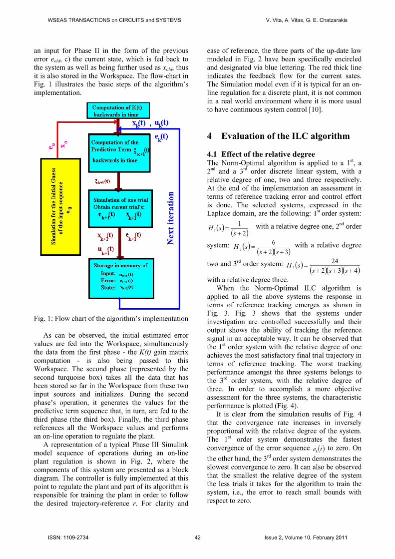
it is also stored in the Workspace. The flow-chart in

Fig. 1 illustrates the basic steps of the algorithm’s

implementation.

Fig. 1: Flow chart of the algorithm’s implementation

As can be observed, the initial estimated error

values are fed into the Workspace, simultaneously

the data from the first phase - the K(t) gain matrix

computation - is also being passed to this

Workspace. The second phase (represented by the

second turquoise box) takes all the data that has

been stored so far in the Workspace from these two

input sources and initializes. During the second

phase’s operation, it generates the values for the

predictive term sequence that, in turn, are fed to the

third phase (the third box). Finally, the third phase

references all the Workspace values and performs

an on-line operation to regulate the plant.

A representation of a typical Phase III Simulink

model sequence of operations during an on-line

plant regulation is shown in Fig. 2, where the

components of this system are presented as a block

diagram. The controller is fully implemented at this

point to regulate the plant and part of its algorithm is

responsible for training the plant in order to follow

the desired trajectory-reference r. For clarity and

ease of reference, the three parts of the up-date law

modeled in Fig. 2 have been specifically encircled

and designated via blue lettering. The red thick line

indicates the feedback flow for the current sates.

The Simulation model even if it is typical for an on-

line regulation for a discrete plant, it is not common

in a real world environment where it is more usual

to have continuous system control [10].

4 Evaluation of the ILC algorithm

4.1 Effect of the relative degree The Norm-Optimal algorithm is applied to a 1

st, a

2nd

and a 3rd

order discrete linear system, with a

relative degree of one, two and three respectively.

At the end of the implementation an assessment in

terms of reference tracking error and control effort

is done. The selected systems, expressed in the

Laplace domain, are the following: 1st

order system:

( )( )2

11

+=

ssH with a relative degree one, 2

nd order

system: ( )( )( )32

62

++=

sssH with a relative degree

two and 3rd

order system: ( )( )( )( )432

243

+++=

ssssH

with a relative degree three.

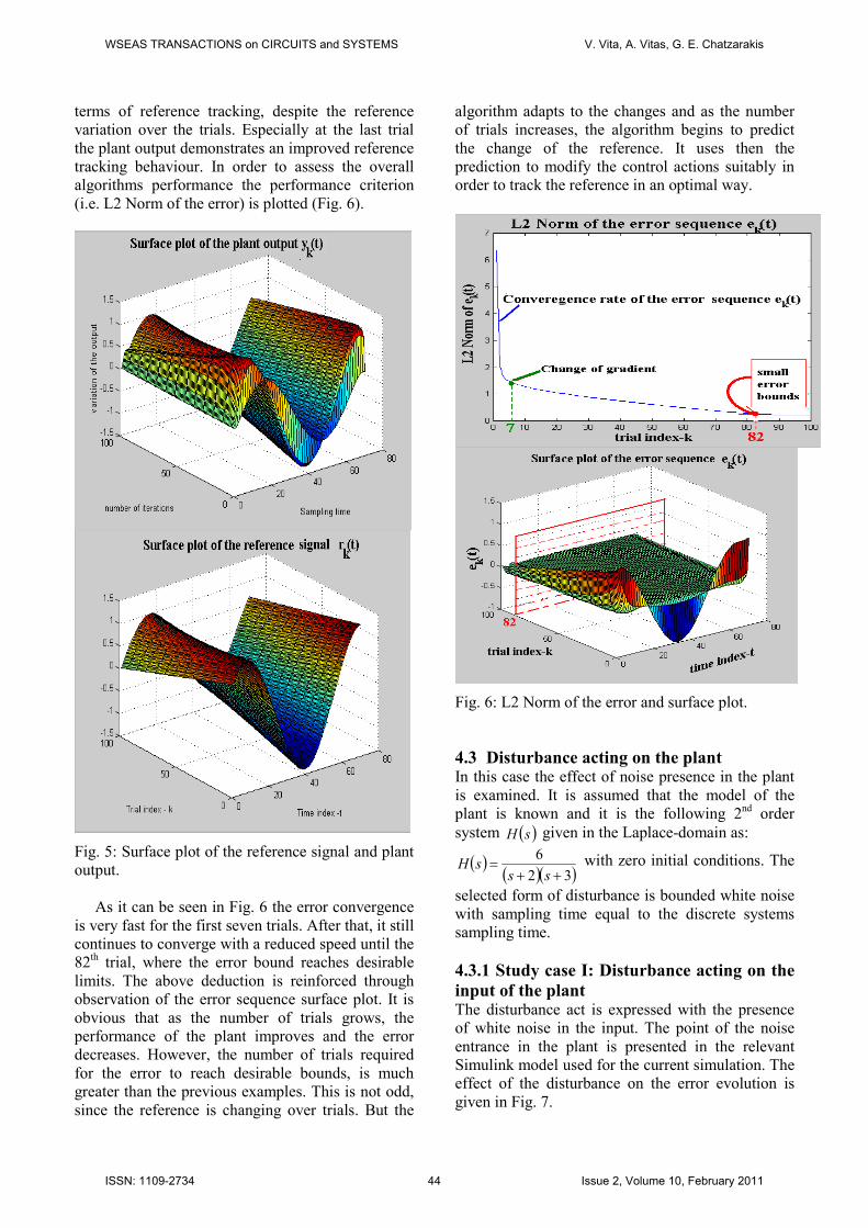
When the Norm-Optimal ILC algorithm is

applied to all the above systems the response in

terms of reference tracking emerges as shown in

Fig. 3. Fig. 3 shows that the systems under

investigation are controlled successfully and their

output shows the ability of tracking the reference

signal in an acceptable way. It can be observed that

the 1st order system with the relative degree of one

achieves the most satisfactory final trial trajectory in

terms of reference tracking. The worst tracking

performance amongst the three systems belongs to

the 3rd

order system, with the relative degree of

three. In order to accomplish a more objective

assessment for the three systems, the characteristic

performance is plotted (Fig. 4).

It is clear from the simulation results of Fig. 4

that the convergence rate increases in inversely

proportional with the relative degree of the system.

The 1st order system demonstrates the fastest

convergence of the error sequence ( )tek to zero. On

the other hand, the 3rd

order system demonstrates the

slowest convergence to zero. It can also be observed

that the smallest the relative degree of the system

the less trials it takes for the algorithm to train the

system, i.e., the error to reach small bounds with

respect to zero.



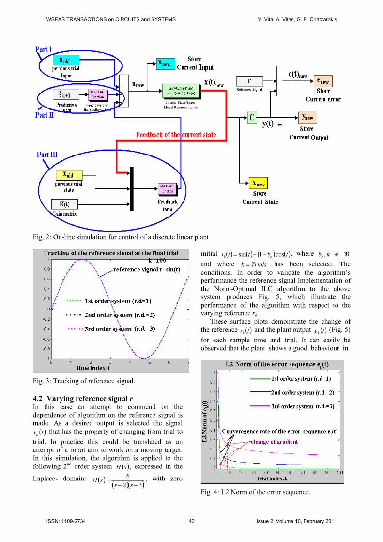
Fig. 2: On-line simulation for control of a discrete linear plant

Fig. 3: Tracking of reference signal.

4.2 Varying reference signal r In this case an attempt to commend on the

dependence of algorithm on the reference signal is

made. As a desired output is selected the signal

( )trk that has the property of changing from trial to

trial. In practice this could be translated as an

attempt of a robot arm to work on a moving target.

In this simulation, the algorithm is applied to the

following 2nd

order system ( )sH , expressed in the

Laplace- domain: ( )( )( )32

6

++=

sssH , with zero

initial ( ) ( ) ( ) ( )tbttr kk cos1sin −+= , where kbk , ∉ ℜ

and where Trialsk = has been selected. The

conditions. In order to validate the algorithm’s

performance the reference signal implementation of

the Norm-Optimal ILC algorithm to the above

system produces Fig. 5, which illustrate the

performance of the algorithm with respect to the

varying reference rk .

These surface plots demonstrate the change of

the reference ( )trk and the plant output ( )tyk

(Fig. 5)

for each sample time and trial. It can easily be

observed that the plant shows a good behaviour in

Fig. 4: L2 Norm of the error sequence.



terms of reference tracking, despite the reference

variation over the trials. Especially at the last trial

the plant output demonstrates an improved reference

tracking behaviour. In order to assess the overall

algorithms performance the performance criterion

(i.e. L2 Norm of the error) is plotted (Fig. 6).

Fig. 5: Surface plot of the reference signal and plant

output.

As it can be seen in Fig. 6 the error convergence

is very fast for the first seven trials. After that, it still

continues to converge with a reduced speed until the

82th trial, where the error bound reaches desirable

limits. The above deduction is reinforced through

observation of the error sequence surface plot. It is

obvious that as the number of trials grows, the

performance of the plant improves and the error

decreases. However, the number of trials required

for the error to reach desirable bounds, is much

greater than the previous examples. This is not odd,

since the reference is changing over trials. But the

algorithm adapts to the changes and as the number

of trials increases, the algorithm begins to predict

the change of the reference. It uses then the

prediction to modify the control actions suitably in

order to track the reference in an optimal way.

Fig. 6: L2 Norm of the error and surface plot.

4.3 Disturbance acting on the plant In this case the effect of noise presence in the plant

is examined. It is assumed that the model of the

plant is known and it is the following 2nd

order

system ( )sH given in the Laplace-domain as:

( )( )( )32

6

++=

sssH with zero initial conditions. The

selected form of disturbance is bounded white noise

with sampling time equal to the discrete systems

sampling time.

4.3.1 Study case I: Disturbance acting on the

input of the plant The disturbance act is expressed with the presence

of white noise in the input. The point of the noise

entrance in the plant is presented in the relevant

Simulink model used for the current simulation. The

effect of the disturbance on the error evolution is

given in Fig. 7.



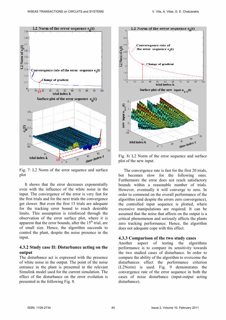
Fig. 7: L2 Norm of the error sequence and surface

plot

It shows that the error decreases exponentially

even with the influence of the white noise in the

input. The convergence of the error is very fast for

the first trials and for the next trials the convergence

get slower. But even the first 15 trials are adequate

for the tracking error bound to reach desirable

limits. This assumption is reinforced through the

observation of the error surface plot, where it is

apparent that the error bounds, after the 15th trial, are

of small size. Hence, the algorithm succeeds to

control the plant, despite the noise presence in the

input.

4.3.2 Study case II: Disturbance acting on the

output The disturbance act is expressed with the presence

of white noise in the output. The point of the noise

entrance in the plant is presented in the relevant

Simulink model used for the current simulation. The

effect of the disturbance on the error evolution is

presented in the following Fig. 8.


plot of the new input.

The convergence rate is fast for the first 20 trials,

but becomes slow for the following ones.

Furthermore the error does not reach satisfactory

bounds within a reasonable number of trials.

However, eventually it will converge to zero. In

order to commend on the overall performance of the

algorithm (and despite the errors zero convergence),

the controlled input sequence is plotted, where

excessive manipulations are required. It can be

assumed that the noise that affects on the output is a

critical phenomenon and seriously affects the plants

zero tracking performance. Hence, the algorithm

does not adequate cope with this effect.

4.3.3 Comparison of the two study cases Another aspect of testing the algorithms

performance is to compare its sensitivity towards

the two studied cases of disturbance. In order to

compare the ability of the algorithm to overcome the

disturbances effect the performance criterion

(L2Norm) is used. Fig. 9 demonstrates the

convergence rate of the error sequence in both the

cases of noise disturbance (input-output acting

disturbance).



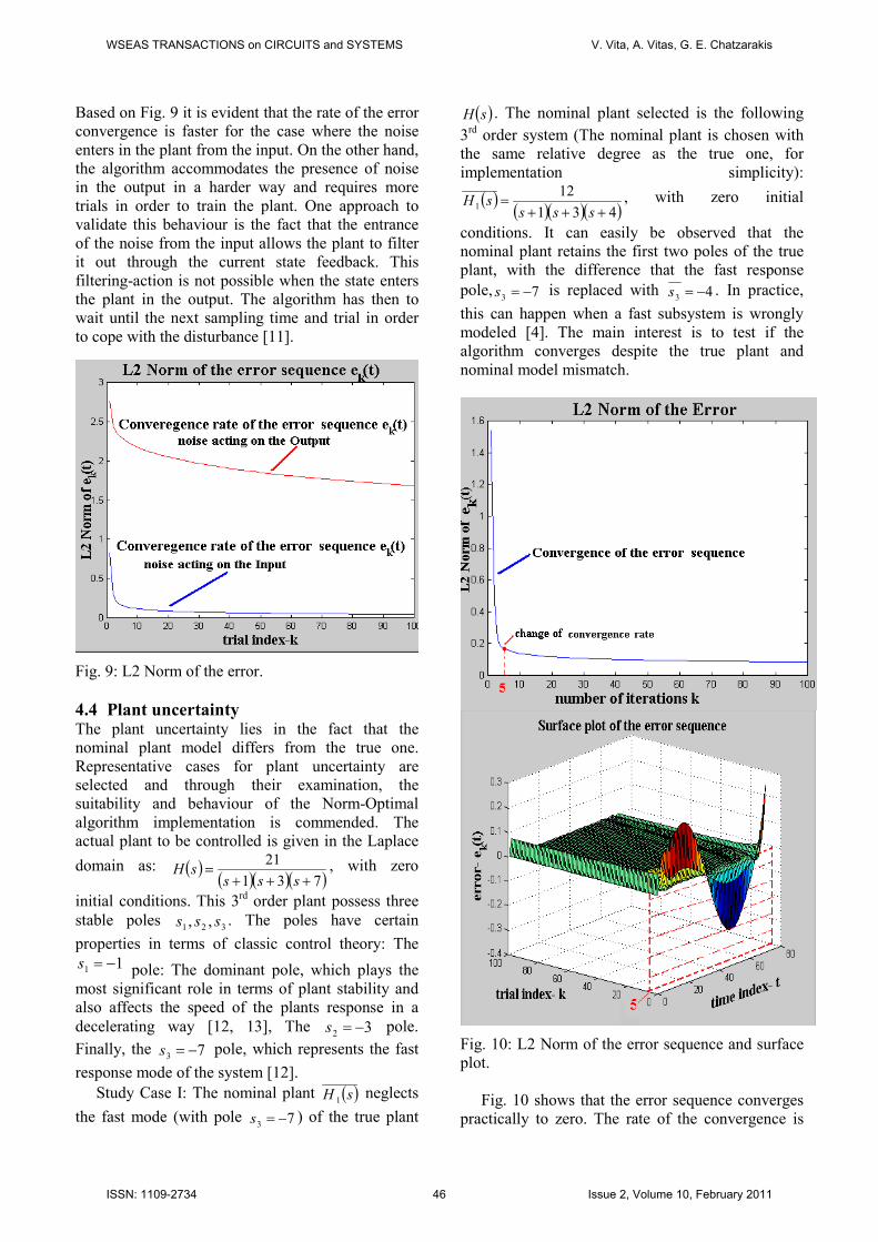
Based on Fig. 9 it is evident that the rate of the error

convergence is faster for the case where the noise

enters in the plant from the input. On the other hand,

the algorithm accommodates the presence of noise

in the output in a harder way and requires more

trials in order to train the plant. One approach to

validate this behaviour is the fact that the entrance

of the noise from the input allows the plant to filter

it out through the current state feedback. This

filtering-action is not possible when the state enters

the plant in the output. The algorithm has then to

wait until the next sampling time and trial in order

to cope with the disturbance [11].

Fig. 9: L2 Norm of the error.

4.4 Plant uncertainty The plant uncertainty lies in the fact that the

nominal plant model differs from the true one.

Representative cases for plant uncertainty are

selected and through their examination, the

suitability and behaviour of the Norm-Optimal

algorithm implementation is commended. The

actual plant to be controlled is given in the Laplace

domain as: ( )( )( )( )731

21

+++=

ssssH , with zero

initial conditions. This 3rd

order plant possess three

stable poles 321 ,, sss . The poles have certain

properties in terms of classic control theory: The

11 −=s pole: The dominant pole, which plays the

most significant role in terms of plant stability and

also affects the speed of the plants response in a

decelerating way [12, 13], The 32 −=s pole.

Finally, the 73 −=s pole, which represents the fast

response mode of the system [12].

Study Case I: The nominal plant ( )sH 1 neglects

the fast mode (with pole 73 −=s ) of the true plant

( )sH . The nominal plant selected is the following

3rd

order system (The nominal plant is chosen with

the same relative degree as the true one, for

implementation simplicity):

( )( )( )( )431

121

+++=

ssssH , with zero initial

conditions. It can easily be observed that the

nominal plant retains the first two poles of the true

plant, with the difference that the fast response

pole, 73 −=s is replaced with 43 −=s . In practice,

this can happen when a fast subsystem is wrongly

modeled [4]. The main interest is to test if the

algorithm converges despite the true plant and

nominal model mismatch.


plot.

Fig. 10 shows that the error sequence converges

practically to zero. The rate of the convergence is



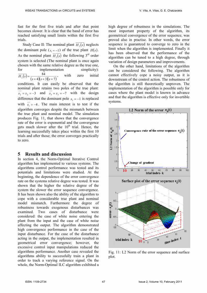
fast for the first five trials and after that point

becomes slower. It is clear that the band of error has

reached satisfying small limits within the first five

trials.

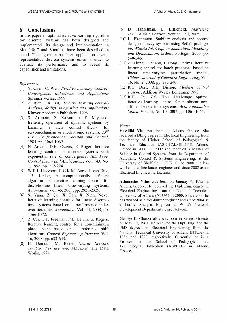
Study Case II: The nominal plant ( )sH 2 neglects

the dominant pole ( 11 −=s ) of the true plant ( )sH .

As the nominal plant ( )sH 2 the following 3

rd order

system is selected (The nominal plant is once again

chosen with the same relative degree as the true one,

for implementation simplicity):

( )( )( )( )734

842

+++=

ssssH , with zero initial

conditions. It can easily be observed that the

nominal plant retains two poles of the true plant:

322 −== ss and 733 −== ss with the design

difference that the dominant pole 11 −=s is replaced

with 41 −=s . The main interest is to test if the

algorithm converges despite the mismatch between

the true plant and nominal model. The simulation

produces Fig. 11, that shows that the convergence

rate of the error is exponential and the convergence

gets much slower after the 10th trial. Hence, the

learning successfully takes place within the first 10

trials and after those; the error converges practically

to zero.

5 Results and discussion In section 4, the Norm-Optimal Iterative Control

algorithm has implemented to various systems. The

algorithms control performance was tested and its

potentials and limitations were studied. At the

beginning, the dependence of the error convergence

rate on the systems relative degree was tested. It was

shown that the higher the relative degree of the

system the slower the error sequence convergence.

It has been shown also the ability of the algorithm to

cope with a considerable true plant and nominal

model mismatch. Furthermore the degree of

robustness towards exogenous disturbances was

examined. Two cases of disturbance were

considered: the case of white noise entering the

plant from the input and the case of white noise

affecting the output. The algorithm demonstrated

high convergence performance in the case of the

input disturbance. For the case of the disturbance

acting in the output, the implementation resulted in

geometrical error convergence; however, the

excessive control input manipulations reduced the

algorithms performance. Another case revealed the

algorithms ability to successfully train a plant in

order to track a varying reference signal. On the

whole, the Norm-Optimal ILC algorithm exhibited a

high degree of robustness in the simulations. The

most important property of the algorithm, its

geometrical convergence of the error sequence, was

proved also in practise. In other words, the error

sequence is guaranteed to converge to zero in the

limit when the algorithm is implemented. Finally it

has been observed that the performance of the

algorithm can be tuned to a high degree, through

variation of design parameters and improvements.

On the other hand, limitations of the algorithm

can be considered the following. The algorithm

cannot effectively cope a noisy output, as it is

downstream of the control action. The robustness of

the algorithm is still theoretically unproven. The

implementation of the algorithm is possible only for

cases where the plant model is known in advance

and that the algorithm is effective only for invertible

systems.


plot.



6 Conclusions In this paper an optimal iterative learning algorithm

for discrete systems has been designed and

implemented. Its design and implementation in

Matlab® 7 and Simulink have been described in

detail. The algorithm has been applied on several

representative discrete systems cases in order to

evaluate its performance and to reveal its

capabilities and limitations.

References:

[1] Y. Chen, C. Wen, Iterative Learning Control-

Convergence, Robustness and Applications

Springer Verlag, 1999.

[2] Z. Bien, J.X. Xu, Iterative learning control-

Analysis, design, integration and applications

Kluwer Academic Publishers, 1998.

[3] S. Arimoto, S. Kawamura, F. Miyazaki,

Bettering operation of dynamic systems by

learning: a new control theory for

servomechanism or mechatronic systems, 23rd

IEEE Conference on Decision and Control,

1984, pp. 1064-1069.

[4] N. Amann, D.H. Owens, E. Roger, Iterative

learning control for discrete systems with

exponential rate of convergence, IEE Proc.

Control theory and Applications, Vol. 143, No.

2, 1996, pp. 217-224.

[5] W.B.J. Hakvoort, R.G.K.M. Aarts, J. van Dijk,

J.B. Jonker, A computationally efficient

algorithm of iterative learning control for

discrete-time linear time-varying systems,

Automatica, Vol. 45, 2009, pp. 2925-2929.

[6] S. Yang, Z. Qu, X. Fan, X. Nian, Novel

iterative learning controls for linear discrete-

time systems based on a performance index

over iterations, Automatica, Vol. 44, 2008, pp.

1366-1372.

[7] Z. Cai, C.T. Freeman, P.L. Lewin, E. Rogers,

Iterative learning control for a non-minimum

phase plant based on a reference shift

algorithm, Control Engineering Practice, Vol.

16, 2008, pp. 633-643.

[8] H. Demuth, M. Beale, Neural Network

Toolbox: For use with MATLAB, The Math

Works, 1994.

[9] D. Hanselman, B. Littlefield, Mastering

MATLAB® 7, Pearson Prentice Hall, 2005.

[10] L. Ekonomou, Stability analysis and control

design of fuzzy systems using Scilab package,

6th WSEAS Int. Conf. on Simulation, Modelling

and Optimization, Lisbon, Portugal, 2006, pp.

540-546.

[11] Z. Xiong, J. Zhang, J. Dong, Optimal iterative

learning control for batch processes based on

linear time-varying perturbation model,

Chinese Journal of Chemical Engineering, Vol.

16, No. 2, 2008, pp. 235-240.

[12] R.C. Dorf, R.H. Bishop, Modern control

systems, Addison Wesley Longman, 1998.

[13] R.H. Chi, Z.S. Hou, Dual-stage optimal

iterative learning control for nonlinear non-

affine discrete-time systems, Acta Automatica

Sinica, Vol. 33, No. 10, 2007, pp. 1061-1065.

Vitae: Vassiliki Vita was born in Athens, Greece. She

received a BEng degree in Electrical Engineering from

the faculty of Higher School of Pedagogical &

Τechnical Education (ASETEM/SELETE), Athens,

Greece in 2000. In 2002 she received a Master of

Science in Control Systems from the Department of

Automatic Control & Systems Engineering, at the

University of Sheffield in U.K. Since 2000 she has

worked as a free-lancer engineer and since 2002 as an

Electrical Engineering Lecturer.

Athanasios Vitas was born on January 9, 1975 in

Athens, Greece. He received the Dipl. Eng. degree in

Electrical Engineering from the National Technical

University of Athens (NTUA) in 2000. Since 2000 he

has worked as a free-lancer engineer and since 2004 as

a Traffic Analysis Engineer at Wind’s Network

Development Department / Core Network.

George E. Chatzarakis was born in Serres, Greece,

on May 20, 1961. He received the Dipl. Eng. and the

PhD degrees in Electrical Engineering from the

National Technical University of Athens (NTUA) in

1986 and 1990, respectively. Currently, he is a

Professor in the School of Pedagogical and

Technological Education (ASPETE) in Athens,

Greece.



Design, implementation and evaluation of an optimal ... · Design, implementation and evaluation of...

Documents

Transcript of Design, implementation and evaluation of an optimal ... · Design, implementation and evaluation of...