J. Math. Anal. Appl. 412 (2014) 236–243

Contents lists available at ScienceDirect

Journal of Mathematical Analysis andApplications

www.elsevier.com/locate/jmaa

De Haan type increasing solutions of half-linear differentialequations

Pavel Rehák a,b,∗a Institute of Mathematics, Academy of Sciences CR, Žižkova 22, CZ-61662 Brno, Czech Republicb Faculty of Education, Masaryk University, Porící 31, CZ-60300 Brno, Czech Republic

a r t i c l e i n f o a b s t r a c t

Article history:Received 11 June 2013Available online 21 October 2013Submitted by D. O’Regan

Keywords:Half-linear differential equationIncreasing solutionBeurling slowly varying functionClass GammaRegular variationRapid variation

We study asymptotic behavior of eventually positive increasing solutions to the half-linear equation (r(t)|y′|α−1 sgn y′)′ = p(t)|y|α−1 sgn y, where r, p are positive continuousfunctions and α ∈ (1,∞). We give conditions which guarantee that any such a solutionis in the class Γ (in the de Haan sense). We also discuss regularly varying solutions andconnections with a generalized regular variation and other related concepts. The resultscan be viewed as a half-linear extension of existing statements for linear equations, but insome aspects they are new also in the linear case.

© 2013 Elsevier Inc. All rights reserved.

1. Introduction

Consider the half-linear differential equation(Φ

(y′))′ = p(t)Φ(y), (1)

where p is a positive continuous function on [a,∞) and Φ(u) = |u|α−1 sgn u with α > 1. We study asymptotic behavior ofeventually positive increasing solutions (which always exist and tend to infinity as t → ∞). In particular, we show that if

p− 1α is Beurling slowly varying, then all these solutions belong to the class Γ with ((α − 1)/p)

1α as an auxiliary function;

the class Γ is meant here as a known specific subclass of rapidly varying functions, see below. We point out a connection ofsuch a behavior with a certain generalization of regular variation. A modification of the proof enables us to get conditionsguaranteeing regular variation of all positive increasing solutions to (1). We also offer an extension of the results to theequation(

r(t)Φ(

y′))′ = p(t)Φ(y), (2)

where r, p are positive continuous functions on [a,∞) with∫ ∞

a r1−β(s)ds = ∞, β being the conjugate number to α, i.e.,1α + 1

β= 1. Our main result for Eq. (1) can be understood as a half-linear extension of the existing results for the linear

equation

y′′ = p(t)y, (3)

* Correspondence to: Institute of Mathematics, Academy of Sciences CR, Žižkova 22, CZ-61662 Brno, Czech Republic.E-mail address: rehak@math.cas.cz.

0022-247X/$ – see front matter © 2013 Elsevier Inc. All rights reserved.http://dx.doi.org/10.1016/j.jmaa.2013.10.048

P. Rehák / J. Math. Anal. Appl. 412 (2014) 236–243 237

which is the special case of (1) when α = 2. Some of the additional related observations are however new even in the linearcase.

The paper is organized as follows. In the next section we briefly present information on basic classification of nonoscil-latory (increasing) solutions to (2), and recall the concept of regularly, rapidly, and (Beurling) slowly varying functions, andfunctions in the class Γ . Section 3 also consists of several paragraphs: First we prove that increasing solutions to (1) arein Γ . Then we deal with regularly varying solutions. Further we show connections of solutions in Γ with generalized reg-ularly varying functions, and finally we present an extension to Eq. (2). All the results are continuously commented, and acomparison with existing literature is made. The paper is concluded by a brief summary and several suggestions for a futureresearch.

2. Preliminaries

Basic classification of nonoscillatory solutions. A (nontrivial) solution of (2) is said to be nonoscillatory if it is eventually ofone sign. Eq. (2) is said to be nonoscillatory if all its (nontrivial) solutions are nonoscillatory; otherwise is said to be os-cillatory. Since the Sturm type separation theorem extends to the half-linear case, one solution of (2) is (non)oscillatory ifand only if all its solutions are (non)oscillatory. Because of the sign condition on p, Eq. (2) is nonoscillatory by the Sturmtype comparison theorem; it suffices to compare (2) with (r(t)Φ(y′))′ = 0. For a (nonoscillatory) solution y of (2) it holds,y(t)y′(t) > 0 or y(t)y′(t) < 0 eventually. Without loss of generalization we may work just with positive solutions. De-note M

+ = {y: y is a solution of (2), y(t) > 0, y′(t) > 0 for large t}. Under our sign condition, the class M+ is nonempty.

Moreover,{∀(a0,a1) ∈ (0,∞) × (0,∞) ∀t0 sufficiently

large ∃y ∈ M+: y(t0) = a0, y′(t0) = a1.

(4)

Further, denote M+B = {y ∈ M

+: limt→∞ y(t) < ∞} and M+∞ = {y ∈ M

+: limt→∞ y(t) = ∞}. Clearly, M+ = M+B ∪M

+∞ . Set

J =∞∫

a

r1−β(t)

( t∫a

p(s)ds

)β−1

dt and Jr =∞∫

a

r1−β(s)ds.

There hold J < ∞ ⇒ Jr < ∞ and M+B �= ∅ ⇔ J < ∞. Hence,

Jr = ∞ ⇒ (∅ �=)M+ = M+∞. (5)

In the special case of Eq. (1), that is r(t) = 1, the discussed classes will be denoted as M+(1) and M

+∞(1). We recommendthe monograph [4] as a source of many other information on half-differential equations. Basic properties (classification andexistence) of nonoscillatory solutions which we present above are established particularly in [2], see also [4, Section 4.1].

Regularly varying functions and related classes. Recall that a measurable function f : [a,∞) → (0,∞) is called regularlyvarying (at infinity) of index ϑ if

limt→∞

f (λt)

f (t)= λϑ for every λ > 0;

we write f ∈ RV(ϑ). If ϑ = 0, then we speak about slowly varying functions; we write f ∈ SV , thus SV = RV(0). A func-tion is called rapidly varying, we write f ∈ RPV(∞) resp. f ∈ RPV(−∞), if the above relation holds with ϑ = ∞ resp.ϑ = −∞; by λ∞ we mean ∞ when λ > 1 and 0 when λ ∈ (0,1), similarly for λ−∞ . While RV functions behave likepower functions (up to a factor which varies “more slowly”), RPV functions have a behavior close to that of exponentialfunctions. For further information on RV and RPV functions we recommend [1,3,5]. The following type of extension ofRV functions, particularly useful in the theory of differential equations, was introduced in [7]. Consider a function ω ∈ C1

which is positive and satisfies ω′(t) > 0 for t ∈ [b,∞) and limt→∞ ω(t) = ∞. A measurable function f : [a,∞) → (0,∞) iscalled regularly varying of index ϑ with respect to ω if f ◦ ω−1 ∈ RV(ϑ); we write f ∈ RVω(ϑ). We denote SVω = RVω(0).It holds, f ∈ RVω(ϑ) if and only if f (t) = ωϑ(t)Lω(t), where Lω ∈ SVω . Further, we have the following representationtheorem: f ∈RVω(ϑ) if and only if

f (t) = ψ(t)exp

{ t∫a

ω′(s)

ω(s)δ(s)ds

},

t � a, for some a > 0, where ψ,δ are measurable and ψ(t) → c ∈ (0,∞), δ(t) → ϑ as t → ∞. If ψ(t) ≡ c, then f iscalled normalized regularly varying with respect to ω; we write f ∈ NRVω(ϑ). Clearly, RV id(ϑ) = RV(ϑ). The same holdsfor normalized case, i.e., NRV id(ϑ) = NRV(ϑ). Regularly and rapidly varying functions has been successfully applied instudying asymptotic properties of differential and difference equations, see e.g. [7–11] and the references therein.

238 P. Rehák / J. Math. Anal. Appl. 412 (2014) 236–243

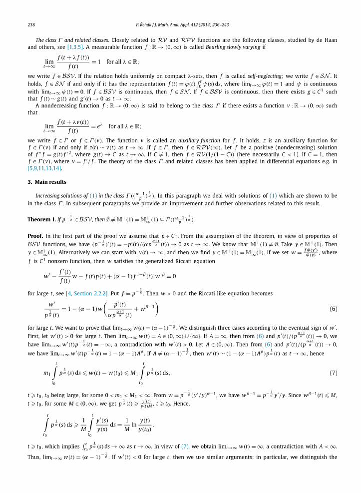
The class Γ and related classes. Closely related to RV and RPV functions are the following classes, studied by de Haanand others, see [1,3,5]. A measurable function f : R→ (0,∞) is called Beurling slowly varying if

limt→∞

f (t + λ f (t))

f (t)= 1 for all λ ∈ R;

we write f ∈ BSV . If the relation holds uniformly on compact λ-sets, then f is called self-neglecting; we write f ∈ SN . Itholds, f ∈ SN if and only if it has the representation f (t) = ϕ(t)

∫ t0 ψ(s)ds, where limt→∞ ϕ(t) = 1 and ψ is continuous

with limt→∞ ψ(t) = 0. If f ∈ BSV is continuous, then f ∈ SN . If f ∈ BSV is continuous, then there exists g ∈ C1 suchthat f (t) ∼ g(t) and g′(t) → 0 as t → ∞.

A nondecreasing function f : R → (0,∞) is said to belong to the class Γ if there exists a function v : R → (0,∞) suchthat

limt→∞

f (t + λv(t))

f (t)= eλ for all λ ∈R;

we write f ∈ Γ or f ∈ Γ (v). The function v is called an auxiliary function for f . It holds, z is an auxiliary function forf ∈ Γ (v) if and only if z(t) ∼ v(t) as t → ∞. If f ∈ Γ , then f ∈ RPV(∞). Let f be a positive (nondecreasing) solutionof f ′′ f = g(t) f ′ 2, where g(t) → C as t → ∞. If C �= 1, then f ∈ RV(1/(1 − C)) (here necessarily C < 1). If C = 1, thenf ∈ Γ (v), where v = f ′/ f . The theory of the class Γ and related classes has been applied in differential equations e.g. in[5,9,11,13,14].

3. Main results

Increasing solutions of (1) in the class Γ ((α−1p )

1α ). In this paragraph we deal with solutions of (1) which are shown to be

in the class Γ . In subsequent paragraphs we provide an improvement and further observations related to this result.

Theorem 1. If p− 1α ∈ BSV , then ∅ �= M

+(1) =M+∞(1) ⊆ Γ ((α−1

p )1α ).

Proof. In the first part of the proof we assume that p ∈ C1. From the assumption of the theorem, in view of properties of

BSV functions, we have (p− 1α )′(t) = −p′(t)/(αp

α+1α (t)) → 0 as t → ∞. We know that M

+(1) �= ∅. Take y ∈ M+(1). Then

y ∈ M+∞(1). Alternatively we can start with y(t) → ∞, and then we find y ∈ M

+(1) = M+∞(1). If we set w = f Φ(y′)

Φ(y), where

f is C1 nonzero function, then w satisfies the generalized Riccati equation

w ′ − f ′(t)f (t)

w − f (t)p(t) + (α − 1) f 1−β(t)|w|β = 0

for large t , see [4, Section 2.2.2]. Put f = p− 1β . Then w > 0 and the Riccati like equation becomes

w ′

p1α (t)

= 1 − (α − 1)w

(p′(t)

αpα+1α (t)

+ wβ−1)

(6)

for large t . We want to prove that limt→∞ w(t) = (α−1)− 1

β . We distinguish three cases according to the eventual sign of w ′ .First, let w ′(t) > 0 for large t . Then limt→∞ w(t) = A ∈ (0,∞) ∪ {∞}. If A = ∞, then from (6) and p′(t)/(p

α+1α (t)) → 0, we

have limt→∞ w ′(t)p− 1α (t) = −∞, a contradiction with w ′(t) > 0. Let A ∈ (0,∞). Then from (6) and p′(t)/(p

α+1α (t)) → 0,

we have limt→∞ w ′(t)p− 1α (t) = 1 − (α − 1)Aβ . If A �= (α − 1)

− 1β , then w ′(t) ∼ (1 − (α − 1)Aβ)p

1α (t) as t → ∞, hence

m1

t∫t0

p1α (s)ds � w(t) − w(t0) � M1

t∫t0

p1α (s)ds, (7)

t � t0, t0 being large, for some 0 < m1 < M1 < ∞. From w = p− 1β (y′/y)α−1, we have wβ−1 = p− 1

α y′/y. Since wβ−1(t) � M ,

t � t0, for some M ∈ (0,∞), we get p1α (t) � y′(t)

y(t)M , t � t0. Hence,

t∫t0

p1α (s)ds � 1

M

t∫t0

y′(s)

y(s)ds = 1

Mln

y(t)

y(t0),

t � t0, which implies∫ t

t0p

1α (s)ds → ∞ as t → ∞. In view of (7), we obtain limt→∞ w(t) = ∞, a contradiction with A < ∞.

Thus, limt→∞ w(t) = (α − 1)− 1

β . If w ′(t) < 0 for large t , then we use similar arguments; in particular, we distinguish the

P. Rehák / J. Math. Anal. Appl. 412 (2014) 236–243 239

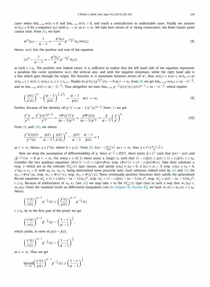
cases when limt→∞ w(t) = 0 and limt→∞ w(t) > 0, and reach a contradiction in undesirable cases. Finally we assumew ′(tn) = 0 for a sequence {tn} with tn → ∞ as n → ∞. We take here zeroes of w ′ being consecutive; the finite cluster pointcannot exist. From (6), we have

wβ(tn) − 1

α − 1= − p′(tn)

αp− α+1

α (tn)w(tn). (8)

Hence, w(t) hits the positive real root of the equation

|λ|β − 1

α − 1= − p′(tn)

αp− α+1

α (tn)λ

at each t = tn . The positive root indeed exists; it is sufficient to realize that the left hand side of the equation representsa parabola like curve symmetric w.r.t. the vertical axis, and with the negative minimum, while the right hand side isa line which goes through the origin. The function w is monotone between zeroes of w ′ , thus w(tn) � w(t) � w(tn+1) or

w(tn+1) � w(t) � w(tn), tn � t � tn+1. Thanks to p′(t)/(pα+1α (t)) → 0 as t → ∞, from (8) we get limn→∞ w(tn) = (α−1)

− 1β ,

and so limt→∞ w(t) = (α − 1)− 1

β . Thus altogether we have limt→∞ p− 1β (t)(y′(t)/y(t))α−1 = (α − 1)

− 1β , which implies

(y(t)

y′(t)

)α

∼(

α − 1

p(t)

) 1β

· αα−1

= α − 1

p(t)as t → ∞. (9)

Further, because of the identity (Φ(y′))′ = (α − 1)y′′|y′|α−2, from (1) we get

y′′ y

y′ 2= y′′ y(y′)α−2

y′ α = (Φ(y′))′ y

(α − 1)y′ α = pΦ(y)y

(α − 1)y′ α = p

α − 1

(y

y′

)α

. (10)

From (9) and (10), we obtain

y′′(t)y(t)

y′ 2(t)= p(t)

α − 1

(y(t)

y′(t)

)α

∼ p(t)

α − 1· α − 1

p(t)= 1

as t → ∞. Hence, y ∈ Γ (h), where h = y/y′ . From (9), h(t) ∼ ( α−1p(t) )

1α as t → ∞, thus y ∈ Γ ((α−1

p )1α ).

Now we drop the assumption of differentiability of p. Since p− 1α ∈ BSV , there exists p ∈ C1 such that p(t) ∼ p(t) and

(p− 1α )′(t) → 0 as t → ∞. For every ε ∈ (0,1) there exists a (large) t0 such that (1 − ε)p(t) � p(t) � (1 + ε)p(t), t � t0.

Consider the two auxiliary equations (Φ(u′))′ = (1 + ε)p(t)Φ(u) resp. (Φ(v ′))′ = (1 − ε)p(t)Φ(v). Take their solutions uresp. v which are in the relevant M

+∞(1) type classes, and satisfy u(t0) = u0 > 0, u′(t0) = u1 > 0 resp. v(t0) = v0 > 0,v ′(t0) = v1 > 0, with u0, u1, v0, v1 being determined more precisely later. Such solutions indeed exist by (4) and (5). Setwu = Φ(u′/u), resp. w v = Φ(v ′/v), resp. w y = Φ(y′/y). These (eventually positive) functions then satisfy the generalizedRiccati equations w ′

u = (1 + ε)p(t) − (α − 1)|wu |β , resp. w ′v = (1 − ε)p(t) − (α − 1)|w v |β , resp. w ′

y = p(t) − (α − 1)|w y |β ,t � t0. Because of arbitrariness of v0, v1 (see (4)) we may take v in the M

+∞(1) type class in such a way that w v(t0) �w y(t0). From the standard result on differential inequalities (see [6, Chapter III, Section 4]), we have w v(t) � w y(t), t � t0.Hence,(

v ′(t)v(t)

)α−1

p− 1β (t) �

(y′(t)y(t)

)α−1

p− 1β (t),

t � t0. As in the first part of the proof, we get

(v ′(t)v(t)

)α−1

p− 1β (t) ∼

(1 − ε

α − 1

) 1β

,

which yields, in view of p(t) ∼ p(t),

(v ′(t)v(t)

)α−1

p− 1β (t) ∼

(1 − ε

α − 1

) 1β

as t → ∞. Thus we get

lim inft→∞

(y′(t)y(t)

)α−1

p− 1β (t)�

(1 − ε

α − 1

) 1β

.

240 P. Rehák / J. Math. Anal. Appl. 412 (2014) 236–243

Analogously, examining wu , we get

lim supt→∞

(y′(t)y(t)

)α−1

p− 1β (t) �

(1 + ε

α − 1

) 1β

.

Since ε ∈ (0,1) was arbitrary, we obtain limt→∞(y′(t)/y(t))α−1 p− 1β (t) = (α − 1)

− 1β . The rest of the proof is the same as in

the previous part. �Remark 1. Results in the spirit of Theorem 1 for linear equation (3) were obtained in [5,11,12,14]. Recall that Γ ⊂RPV(∞).Thus we should mention also the book by Maric [9], where the condition

t

λt∫t

p(s)ds → ∞

as t → ∞ is proved to be necessary and sufficient for decreasing and increasing solutions of (3) to be rapidly varying; theproof is presented just for decreasing solutions. Concerning an extension of Maric’s result to half-linear equation (1), theauthor has not found any paper on this topic, except of [10], where the discrete counterpart is considered and only decreas-ing solutions are examined. As for differential equations, there is only a mention made by prof. Kusano at CDDE conferencein 2000 about an allegedly existing statement which extends Maric’s theorem for the case of decreasing solutions to (1),with emphasizing that the case of increasing solutions of (1) is an open problem (both, the existence of an RPV increasingsolution as well as the fact that all increasing solutions are RPV). Theorem 1, in fact, offers a condition guaranteeing thatany eventually positive increasing solution (which indeed exists) is rapidly varying and, moreover, its asymptotic behavior

is more specified. Observe that this sufficient condition, for a differentiable p having the form (p− 1α )′(t) → 0 as t → ∞,

implies the one of Maric type modified for (1), namely

tα−1

λt∫t

p(s)ds → ∞.

Finally, consider the special case when p(t) → C ∈ (0,∞) as t → ∞. Then, from the proof of Theorem 1 we see that

y ∈ M+ satisfies limt→∞ y′(t)/y(t) = ((α − 1)/C)− 1

α . Thus, from this point of view, the solution y can be understood as ofPoincaré–Perron type. Such a behavior, along with numerous refinements, is studied quite extensively for linear equationsor systems also in the present; as one of the pioneering works can be regarded the classical paper [15]. So as a by-productof our results, we offer — to some extent — a half-linear extension of this result in the second order case.

Regularly varying solutions. Let p be differentiable. In the previous considerations we assumed that limt→∞(p− 1α )′(t) = 0.

Now assume that the limit is nonzero, i.e., limt→∞ p′(t)/p− α+1α = C �= 0. Denote by the positive root of

| |β + C

α − 1

α − 1= 0.

It is easy to see that the root indeed exists and �= (α − 1)− 1

β . Take y ∈ M+(1). Similar arguments as in the first part of

the proof of Theorem 1 yield

(y′(t)y(t)

)α−1

p− 1β (t) ∼

as t → ∞. Using this relation along with (10), we get

limt→∞

y′′(t)y(t)

y′ 2(t)= 1

(α − 1) β�= 1.

We (naturally) assume that C < 0. Then > (α − 1)−β , and so

limt→∞

y′′(t)y(t)

y′ 2(t)= σ < 1,

where σ = 1/((α − 1) β). Hence, y ∈ RV(1/(1 − σ)), or y ∈ RV(−α β−1/C). Thanks to convexity of solutions to (1), weget normalized regular variation. Thus we have proved the following theorem.

P. Rehák / J. Math. Anal. Appl. 412 (2014) 236–243 241

Theorem 2. Let p be differentiable and limt→∞ p′(t)/p− α+1α (t) = C < 0. Then

∅ �=M+(1) = M

+∞(1) ⊆ NRV(−α β−1/C

),

where is the positive root of

| |β + C

α − 1

α − 1= 0.

Remark 2. From the results of [8] (which are originally formulated for (2) with no sign condition on p) it follows that (1)possesses solutions yi with yi ∈ RV(Φ−1(λi)), i = 1,2, where λ1 < 0 < λ2 are the roots of |λ|β − λ − A = 0 if and only

if limt→∞ tα−1∫ ∞

t p(s)ds = A(< 0). Observe that p′(t)p− α+1α (t) ∼ C(< 0) implies tα−1

∫ ∞t p(s)ds ∼ (−α/C)α/(α − 1) as

t → ∞. Further, it is easy to see that λ2 = (−α/C)α−1 , and so — as expected — the indices of regular variation of increasingsolutions in both the results coincide. Note that the integral condition from [8] is more general than our condition. On theother hand, the fixed point approach used in [8] guarantees the existence of at least one positive increasing RV solution,while our result says that all positive increasing solutions are regularly varying.

A connection with generalized regular variation. First observe, that if a positive function f ∈ C1 satisfies τ (t) f ′(t)/ f (t) ∼ϑ ∈ R as t → ∞, where τ is positive continuous with

∫ ∞a (1/τ (s))ds = ∞, then f ∈ NRVω(ϑ), where ω(t) =

exp{∫ ta 1/τ (s)ds}. This fact easily follows from the representation theorem. Assume now p− 1

α ∈ BSV , and take y ∈ M+(1).

From the proof of Theorem 1, we have y′(t)/y(t) ∼ (p(t)/(α − 1))1α as t → ∞. Set τ (t) = p− 1

α (t). Then ln y(t) ∼N

∫ tt0

(1/τ (s))ds as t → ∞, for some N ∈ (0,∞), which implies∫ ∞

t0(1/τ (s))ds = ∞. If we set ϑ = (α − 1)− 1

α , then y

satisfies τ (t)y′(t)/y(t) ∼ ϑ as t → ∞ and now it is easy to see that

y ∈ NRVω

((α − 1)−

1α), where ω(t) = exp

{ t∫a

p1α (s)ds

}.

The statement of Theorem 1 can therefore be reformulated in terms of generalized RV functions. In particular, we get

M+(1) ⊆ NRVω

((α − 1)−

1α)

with the above defined ω.

Extension to Eq. (2). Consider now more general equation (2), where r satisfies∫ ∞

a r1−β(s)ds = ∞. Set R(t) = ∫ ta r1−β(s)ds

and denote by R−1 its inversion. Let us introduce new independent variable s = ξ(t) and new function u(s) = y(ξ−1(s)) =y(t), where ξ ∈ C1, ξ(t) > 0, ξ ′(t) > 0, t ∈ [a,∞), and ξ(t) → ∞ as t → ∞. Then d

dt = ξ ′(ξ−1(s)) dds , and (2) is transformed

into

d

ds

(r(ξ−1(s)

)Φ

(ξ ′(ξ−1(s)

))Φ

(du

ds

))= p(ξ−1(s))

ξ ′(ξ−1(s))Φ(u). (11)

Set ξ(t) = R(t). Then ξ ′(ξ−1(s)) = r1−β(R−1(s)) and (11) becomes

d

ds

(Φ

(du

ds

))= p(s)Φ(u), (12)

where p(s) = p(R−1(s))r1−β (R−1(s))

. Take a solution y of (2) such that y ∈ M+ . Then y ∈ M

+∞ , and — after the transformation — the

corresponding solution u of (12) satisfies u(s) → ∞ as s → ∞ with dds u(s) > 0 eventually. If we now assume p− 1

α ∈ BSV ,then as in the proof of Theorem 1 we get

dds u(s)

u(s)∼

(p(s)

α − 1

) 1α

as s → ∞. Since dds = rβ−1(t) d

dt , the last asymptotic relation yields

rβ−1(t)y′(t)y(t)

∼(

rβ−1(t)p(t)

α − 1

) 1α

as t → ∞, which yields y′(t)/y(t) ∼ 1/Q (t) as t → ∞, where Q (t) = [p(t)/((α − 1)r(t))]− 1α . Take ε > 0 and t0 such that

242 P. Rehák / J. Math. Anal. Appl. 412 (2014) 236–243

1 − ε

Q (t)� y′(t)

y(t)� 1 + ε

Q (t),

t � t0. Assume Q ∈ BSV . Then Q ∈ SN , because of continuity. Let λ > 0 and take the integral between t and t + λQ (t),for which by the local uniform convergence the following relation holds,

t+λQ (t)∫t

1

Q (v)dv =

λ∫0

Q (t)

Q (t + zQ (t))dz → λ

as t → ∞. Thus we get

(1 − ε)λ � lim inft→∞ ln

y(t + λQ (t))

y(t)� lim sup

t→∞ln

y(t + λQ (t))

y(t)� (1 + ε)λ.

Letting ε → 0 we come to y ∈ Γ (Q ). The above considerations are made under the assumptions p ∈ BSV and Q ∈ BSV . Ifwe assume p, r differentiable, then — after some rearrangement in the former equality — we get

d

dsp− 1

α (s) =(

− 1

α

(r

p

) α+1α p′r − pr′

r2+ (1 − β)

(r

p

) 1α r′

r

)◦ R−1(s)

and

(α − 1)−1α Q ′(t) =

(− 1

α

(r

p

) α+1α p′r − pr′

r2

)(t).

Thus we see that in the case of differentiable coefficients it is sufficient to require the expressions on the right hand sidesto tend to zero as s resp. t tends to infinity. So we have obtained the following result, which extends Theorem 1.

Theorem 3. Let∫ ∞

a r1−β(s)ds = ∞. Denote R(t) = ∫ ta r1−β(s)ds. Then any of the two sets of conditions

(i) (p

r1−β )− 1α ◦ R−1 ∈ BSV , ( p

r )− 1α ∈ BSV ,

or

(ii) p, r are differentiable, (( pr )− 1

α )′(t) → 0 and ((pr )− 1

α r′r )(t) → 0 as t → ∞

guarantees

∅ �=M+ = M

+∞ ⊆ Γ

(((α − 1)r

p

) 1α)

.

Remark 3. (i) A closer examination of the above observations reveals that the part of the proof of Theorem 1 starting with(9) can alternatively be shown via a different method, namely the one which was used to obtain Theorem 3. Because of thegeneral coefficient r in the differential term, the result for Eq. (2) is new also in the linear case.

(ii) The asymptotic conditions in the second part of Theorem 3 can be relaxed to ((pr )− 1

α )′(t) → 0 and ((p

r1−β )− 1α )′(t) ·

rβ−1(t) → 0 as t → ∞.

4. Concluding remarks

We have obtained a direct half-linear extension of certain results dealing with increasing solutions in the class Γ ofsecond order linear equations. At the same time, we offer additional related observations which are improvements or com-plements even in specific cases. There are also new information about the connection of the class Γ with generalizedregularly varying solutions and Poincaré–Perron type solutions. Worthy of note is the fact that our results can be appliedto PDE’s with p-Laplacian when studying their radially symmetric solutions. We believe that some of the ideas of this pa-per can be used for a further investigation of half-linear equations in the framework of de Haan type classes and relatedasymptotic behavior. For illustration, let us mention the following several suggestions for a future research. A complementto the requirement in Theorem 3 is the condition

∫ ∞a r1−β(s)ds < ∞. In contrast to linear equations, where a transforma-

tion of dependent variable enables us to transform this problem into the divergent integral case, we must proceed directlywith this setting in the half-linear case. Note that the condition

∫ ∞a r1−β(s)ds < ∞ may strongly affect the existence in the

class M+∞ , see [4, Chapter 4.1]. Another topic which would be of interest is to obtain a more precise information about the

rate of convergence of y(t+λv(t)) for a solution y of (2); see [12,14] for the corresponding considerations in the linear case.

y(t)

P. Rehák / J. Math. Anal. Appl. 412 (2014) 236–243 243

Acknowledgments

The author is supported by the GACR grant No. 201/10/1032 and by RVO 67985840.

References

[1] N.H. Bingham, C.M. Goldie, J.L. Teugels, Regular Variation, Encyclopedia Math. Appl., vol. 27, Cambridge University Press, 1987.[2] M. Cecchi, Z. Došlá, M. Marini, On nonoscillatory solutions of differential equations with p-Laplacian, Adv. Math. Sci. Appl. 11 (2001) 419–436.[3] L. de Haan, On Regular Variation and Its Applications to the Weak Convergence of Sample Extremes, Mathematisch Centrum, Amsterdam, 1970.[4] O. Došlý, P. Rehák, Half-Linear Differential Equations, Elsevier, North-Holland, 2005.[5] J.L. Geluk, L. de Haan, Regular Variation, Extensions and Tauberian Theorems, CWI Tract, vol. 40, Centrum voor Wiskunde en Informatica, Amsterdam,

1987.[6] P. Hartman, Ordinary Differential Equations, Society for Industrial and Applied Mathematics, 2002.[7] J. Jaroš, T. Kusano, Self-adjoint differential equations and generalized Karamata functions, Bull. Cl. Sci. Math. Nat. Sci. Math. CXXIX (29) (2004) 25–60.[8] J. Jaroš, T. Kusano, T. Tanigawa, Nonoscillatory half-linear differential equations and generalized Karamata functions, Nonlinear Anal. 64 (2006) 762–787.[9] V. Maric, Regular Variation and Differential Equations, Lecture Notes in Math., vol. 1726, Springer-Verlag, Berlin, Heidelberg, New York, 2000.

[10] S. Matucci, P. Rehák, Rapidly varying decreasing solutions of half-linear difference equations, Math. Comput. Modelling 49 (2009) 1692–1699.[11] E. Omey, Regular variation and its applications to second order linear differential equations, Bull. Soc. Math. Belg. Sér. B 33 (1981) 207–229.[12] E. Omey, Rapidly varying behaviour of the solutions to a second order linear differential equation, in: Proc. of the 7th Int. Coll. on Differential Equations,

Plovdiv, August 18–23, 1996, VSP, Utrecht, 1997, pp. 295–303.[13] E. Omey, A note on the solutions of r′′(x)r(x) = g(x)r′ 2(x), in: Proc. of the 9th Int. Coll. on Differential Equations, Plovdiv, August 18–23, 1998, VSP,

Utrecht, 1999, pp. 293–298.[14] E. Omey, On the class gamma and related classes of functions, retrieved April 19, 2013, from www.edwardomey.com/nonsave/OmeyBeurlingJuli2011

Final.pdf.[15] H. Poincaré, Sur les equations lineaires aux differentielles ordinaires et aux differences finies, Amer. J. Math. 7 (1885) 203–258 (in French).