The SCUBA HAlf Degree Extragalactic Survey – VI....

Mon. Not. R. Astron. Soc. 384, 1597–1610 (2008) doi:10.1111/j.1365-2966.2007.12808.x

The SCUBA HAlf Degree Extragalactic Survey – VI. 350-μm mapping of

submillimetre galaxies

Kristen Coppin,1,2� Mark Halpern,1 Douglas Scott,1 Colin Borys,3 James Dunlop,4

Loretta Dunne,5 Rob Ivison,4,6 Jeff Wagg,7,8 Itziar Aretxaga,8 Elia Battistelli,1

Andrew Benson,9 Andrew Blain,9 Scott Chapman,9 Dave Clements,10 Simon Dye,11

Duncan Farrah,12 David Hughes,8 Tim Jenness,13 Eelco van Kampen,14 Cedric Lacey,2

Angela Mortier,4 Alexandra Pope,1 Robert Priddey,15 Stephen Serjeant,16 Ian Smail,2

Jason Stevens15 and Mattia Vaccari17

1Department of Physics & Astronomy, University of British Columbia, 6224 Agricultural Road, Vancouver, British Columbia, Canada V6T 1Z12Institute for Computational Cosmology, University of Durham, South Road, Durham DH1 3LE3Department of Astronomy & Astrophysics, University of Toronto, 50 St George Street, Toronto, Ontario, Canada M5S 3H44Institute for Astronomy, University of Edinburgh, Royal Observatory, Blackford Hill, Edinburgh EH9 3HJ5The Centre for Astronomy & Particle Theory, The School of Physics & Astronomy, University of Nottingham, University Park, Nottingham NG7 2RD6UK ATC, Royal Observatory, Blackford Hill, Edinburgh EH9 3HJ7National Radio Astronomy Observatory, PO Box 0, Socorro, NM 87801, USA8Instituto Nacional de Astrofısica, Optica y Electronica, Apartado Postal 51 y 216, 72000 Puebla, Pue., Mexico9Caltech, 1200 E. California Blvd, Pasadena, CA 91125-0001, USA10Astrophysics Group, Blackett Laboratory, Imperial College, Prince Consort Road, London SW7 2BW11School of Physics and Astronomy, Cardiff University, 5 The Parade, Cardiff CF24 3YB12Department of Astronomy, Cornell University, Space Sciences Building, Ithaca, NY 14853, USA13Joint Astronomy Centre, 660 N. A’ohoku Place, University Park, Hilo, HI 96720, USA14Institute for Astro- and Particle Physics, University of Innsbruck, Technikerstr. 25, A-6020 Innsbruck, Austria15Centre for Astrophysics Research, Science and Technology Research Institute, University of Hertfordshire, College Lane,Hatfield, Hertfordshire AL10 9AB16Department of Physics, The Open University, Milton Keynes MK7 6AA17Department of Astronomy, University of Padova, Vicolo dell’Osservatorio 2, 35122 Padova, Italy

Accepted 2007 December 4. Received 2007 December 4; in original form 2007 May 21

ABSTRACT

A follow-up survey using the Submillimetre High-Angular Resolution Camera (SHARC-II)at 350 μm has been carried out to map the regions around several 850-μm-selected sourcesfrom the Submillimetre HAlf Degree Extragalactic Survey (SHADES). These observationsprobe the infrared (IR) luminosities and hence star formation rates in the largest existing,most robust sample of submillimetre galaxies (SMGs). We measure 350-μm flux densities for24 850-μm sources, seven of which are detected at ≥2.5σ within a 10 arcsec search radiusof the 850-μm positions. When results from the literature are included the total number of350-μm flux density constraints of SHADES SMGs is 31, with 15 detections. We fit a modifiedblackbody to the far-IR (FIR) photometry of each SMG, and confirm that typical SMGs aredust-rich (Mdust � 9 × 108 M�), luminous (LFIR � 2 × 1012 L�) star-forming galaxies withintrinsic dust temperatures of �35 K and star formation rates of �400 M� yr−1. We havemeasured the temperature distribution of SMGs and find that the underlying distribution isslightly broader than implied by the error bars, and that most SMGs are at 28 K with afew hotter. We also place new constraints on the 350-μm source counts, N350(>25 mJy) ∼200–500 deg−2.

Key words: surveys – galaxies: formation – galaxies: high-redshift – galaxies: starburst –cosmology: observations – submillimetre.

�E-mail: [email protected]

C© 2008 The Authors. Journal compilation C© 2008 RAS

1598 K. Coppin et al.

1 IN T RO D U C T I O N

The Submillimetre Common-User Bolometer Array (SCUBA)HAlf Degree Extragalactic Survey (SHADES; Mortier et al. 2005;Coppin et al. 2006) mapped �0.25 deg2 of sky with an rms of 2 mJyat 850 μm with SCUBA (Holland et al. 1999). The area was splitapproximately evenly between the Lockman Hole (LH) and theSubaru-XMM Deep Field (SXDF). Using uniform selection crite-ria, the survey uncovered 120 submillimetre galaxies (SMGs) witha median deboosted flux density of ∼5 mJy (Coppin et al. 2006).The SHADES programme was designed to study the nature andevolution of high star formation rate (SFR) SMGs via a systematicstudy of a well-characterized and statistically meaningful sample.The programme includes an effort to identify members of the sourcelist at other wavelengths using deep follow-up data from the radio(Ivison et al. 2007) to X-ray, in order to characterize the SHADESpopulation and to probe the variation in the star formation and clus-tering with redshift. The relatively precise positions available fromthe radio data greatly aid in identifying secure counterparts at otherwavelengths, which can then be used to provide spectroscopic orphotometric redshifts (Aretxaga et al. 2007) and to categorize thesources.

Even combined with knowledge of source redshift, SCUBA850 μm and millimetre wavelength fluxes do not constrain the totaldust mass of a galaxy because there is an ambiguity between col-umn density and source temperature. The submillimetre (submm)spectral energy distribution (SED) of a luminous dusty galaxy arisesfrom the re-emission at far-infrared (FIR) wavelengths of absorbedoptical/ultraviolet radiation from regions of intense star formation(see e.g. Sanders & Mirabel 1996, and references therein). Typicallythe dust temperature is within a factor of 2 of Td ∼ 40 K (Blain et al.2002), so the rest-frame SED peaks in the range 60–120 μm and theSED is almost a simple power law at the SCUBA wavelengths andlonger.

At a redshift of 〈z〉∼ 2 or 3, typical of SMGs (Chapman et al.2005), the peak of the SED is shifted to be near 350 μm, andthe Submillimetre High Angular Resolution Camera (SHARC-II;Dowell et al. 2003) at the Caltech Submillimetre Observatory (CSO)is very well situated to provide the photometry needed to constrainthe temperatures, and therefore the luminosities and masses, of theSHADES sources.

We have therefore mapped a subset of the SHADES cataloguewith SHARC-II. In this paper we constrain the FIR SEDs of oursample by fitting modified blackbody curves to the FIR photome-try of 31 SHADES SMGs including SHARC-II data at 350 μm.Sections 2 and 3 describe the observations and data reduction.Section 4 presents the 350-μm flux densities of the SHADESgalaxies and the FIR SEDs. Section 5 provides a discussion ofthe results. Conclusions and future prospects are discussed inSection 6. We adopt the cosmological parameters from theWilkinson Microwave Anisotropy Probe (WMAP) fits in Spergelet al. (2003): �� = 0.73, �m = 0.27 and H0 = 71 km s−1 Mpc−1.

2 SU RV E Y D E S I G N A N D O B S E RVAT I O N S

2.1 Instrument description

SHARC-II is a background-limited 350- and 450-μm common-usercontinuum camera with a 3 × 1.5 arcmin2 field of view (FOV) at the10.4-m CSO in Hawaii (Dowell et al. 2003). The dish has a very lowsurface error (10.4-μm rms at 350 μm) due to the active Dish SurfaceOptimization System (Leong 2005) which corrects the primary for

surface imperfections and gravitational deformations as a functionof elevation angle during observations to improve the telescopeefficiency and pointing. The result is that the CSO is probably thebest telescope in the world at shorter submm wavelengths. Theresulting beam size (with good focus and pointing) is 9 arcsec fullwidth at half-maximum (FWHM) at 350 μm.

2.2 Sample selection

120 submm sources have been identified in the SHADES fields(Coppin et al. 2006). Obtaining useful photometry for the full setwould require several hundred hours of excellent weather, so wehave chosen to observe a carefully chosen subset of the SHADEScatalogue. Many sources lie close enough together that multipletargets can be selected within a single SHARC-II FOV. We choseeight of our 14 fields to contain a large fraction of the SHADESclose angular pairs. This is mostly just for efficiency, but there is alsoa small chance that the observations would help measure clusteringin the SHADES catalogue. We chose a deliberate mixture of sourceswith compact, extended or no radio counterparts (Ivison et al. 2007):11 sources with one robust compact radio ID; three sources with tworobust compact radio counterparts; three sources with one extended-looking radio counterpart; and seven sources with no reliable radioID. Choosing targets with this mixture of radio characteristics couldhelp refine the SHADES redshift distribution and test if there is asubpopulation with a high-redshift tail (e.g. Dunlop 2001; Ivison2006).

Two of our fields were also observed by Kovacs et al. (2006)or Laurent et al. (2006) (sources LOCK850.3, LOCK850.1 andLOCK850.41), which allows for cross-calibration and checks ofsystematics in observation and analysis. One field (LOCK44/45)covered two 850-μm source candidates from a preliminarySHADES catalogue which were later eliminated from the officialSHADES catalogue since they were deemed likely to be spurioussources (Coppin et al. 2006). This field is not used in the ensuinganalysis.

2.3 Observations

10 SHADES LH fields were mapped over the course of four su-perb stable weather nights in 2005 March and 2006 February(0.035 < τ 225 GHz < 0.06). Four additional fields were observedin more marginal observing conditions. For each field data werecollected in 10 min scans using a non-connecting Lissajous scanpattern with small amplitudes of typically 20 arcsec in both altitudeand azimuth and a ‘period’ of 15–20 s. Integration times, typicalweather conditions and resulting map depths of each SHARC-IIfield are given in Table 1.

By design, our strategy was to reach a map rms of 3σ � 30 mJyat 350 μm, sufficient to detect or place useful limits on an S850 ∼8 mJy SMG with Td � 40 K at z � 3. Good weather is scarce, and itis important to be as efficient as possible by only integrating down tothe planned noise level. We tracked the effective integrating time oneach source by compensating each 10-min file for zenith angle andatmospheric opacity at 350 μm, as inferred from the τ 350 μm andτ 225 GHz dippers. See Appendix A for details. Typically, 3–4 h ofobservations were required for a map 3 × 1.5 arcmin2 in size.

Pointing, focus checks and calibration were performed hourly onstandard sources in close proximity to the science targets. The samescan pattern was used as for the science targets, but with integrationtimes of only 120–160 s (as typical flux densities are �2 Jy).

C© 2008 The Authors. Journal compilation C© 2008 RAS, MNRAS 384, 1597–1610

SHARC-II follow-up of SHADES sources 1599

Table 1. Summary of the SHARC-II observations and map properties. RA and Dec. (J2000) coordinates are given for the field pointing centre, with each fieldcontaining one or more SHADES sources. The date of observations, weather conditions (mean atmospheric opacity at 350 μm), and the ‘effective’ integrationtimes (see Appendix A; note that this is not the same as the actual time spent on the sky) are listed. Since a large fraction of each map comprises noisy edges,we quote a median value of a ‘trimmed’ noise map containing only pixels with more than 60 per cent of the maximum depth coverage achieved by the centralpixel in the map. Total map areas are also given.

Field SHADES RA Dec. UT date Mean Effective integration time Median rms Map areaname sources (J2000) (J2000) (yy-mm-dd) τ 350 μm (min) (mJy) (arcmin2)

LOCK21/28 21, 28 10h52m57.s3 57◦30′54.′′0 05-02-28/-03-08,09 1.30 8.5 13 3.1LOCK26/32 26 10h52m39.s7 57◦23′16.′′4 05-02-28 0.99 9.3 9 3.1LOCK4/69 4 10h52m05.s5 57◦27′06.′′4 05-02-28 0.88 9.9 10 3.1LOCK3/47 3, 47 10h52m37.s1 57◦24′57.′′5 05-02-28 0.88 1.1 20 3.0LOCK33/42 33, 77 10h51m56.s5 57◦23′05.′′5 05-03-01 0.90 8.9 9 3.1LOCK10/48/64 10, 48, 64 10h52m52.s0 57◦32′51.′′4 05-03-01 0.89 9.8 13 3.7LOCK1/41/63 1, 6, 41, 63 10h51m57.s9 57◦24′60.′′6 05-03-01 0.80 13.7 23 3.9LOCK16/50 16 10h51m49.s3 57◦26′44.′′5 05-03-08 1.33 7.5 17 3.8LOCK22/25 22 10h51m35.s2 57◦33′26.′′9 05-03-08,09 1.52 6.0 17 3.5LOCK44/45 none 10h51m56.s8 57◦28′37.′′9 05-03-09 1.33 4.7 22 3.8LOCK15 15 10h53m19.s1 57◦21′10.′′5 06-02-24 1.52 1.1 55 2.8SXDF1/11 1, 11 02h17m27.s9 −04◦59′38.′′0 04-08-30,31/-09-01 1.83 6.4 14 3.8SXDF3/8 3, 8 02h17m43.s2 −04◦56′12.′′5 04-08-30,31/-09-01 1.81 5.2 15 4.3SXDF17/26 17, 119 02h17m55.s8 −04◦52′50.′′4 05-03-01,03,05,07,08,09 1.39 6.8 17 3.1

The typical pointing rms of 2–3 arcsec at the CSO is a non-negligible fraction of the 9 arcsec beam size, and much care is takento minimize pointing errors. Observations of point-like galaxies,quasars, protostellar sources, H II regions and evolved stars are usedby the CSO staff for constructing a pointing model. The modelpredictions for the calibrators observed before and after scienceobservations are compared to the actual pointing measurements;offsets are calculated and applied to the model pointing predictionsfor the science observations during the map co-addition stage ofthe reduction. This procedure yields a pointing accuracy rms of∼2 arcsec (D. Dowell, private communication).

Flux calibration is performed by comparing the known and mea-sured flux densities and beam sizes obtained for standard calibrationsources. For sources in the SXDF, oCeti (a Mira variable) and oc-casionally OH231 (a protoplanetary nebula) were used as pointingand calibration sources. For sources in the LH, CIT6 (an evolvedstar) was used, and the nearby asteroids Pallas and Egeria whenCIT6 was unavailable. The standards have well-tabulated 350-μmflux densities, which are available from the CSO/SHARC-II cali-bration web page.1 The final calibration is expected to be better than15 per cent, with systematic effects being negligible at that level(CSO staff, private communication).

3 DATA R E D U C T I O N

3.1 Mapmaking and source extraction

We make maps from the raw data and then extract 350-μm fluxesfrom the maps.

The mapmaking data reduction package is CRUSH (Comprehen-sive Reduction Utility for SHARC-II), a JAVA-based tool developedby Kovacs (2006). The software iterates a least-squares algorithmto solve for celestial emission along with instrumental and atmo-spheric contributions to the total power signal. CRUSH accesses theτ 350 μm polynomial fits to obtain a low-noise 350-μm sky opacity-

1 http://www.submm.caltech.edu/∼sharc.

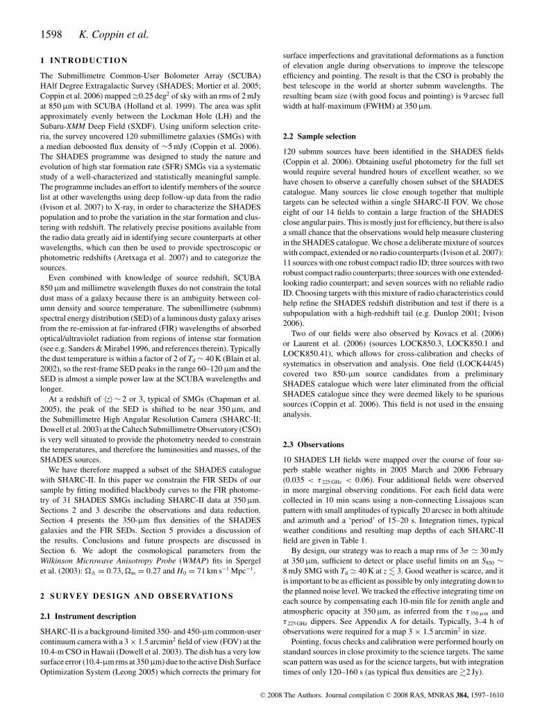
based estimate of the atmospheric signal. Using the ‘deep’ utility,as is recommended for sources fainter than 100 mJy, the maps ofeach field are co-added on a grid of 1.62 × 1.62 arcsec2 pixels. Theouter four rows of pixels are removed automatically by CRUSH sincethey are not sampled sufficiently well to converge to useful mea-surements. The data are fitted with a single Gaussian beam profilewith a FWHM of 9 arcsec. Thumbnails of the reduced maps centredon the SHADES 850-μm positions are shown in Fig. 1. The bulk ofthe structure in these images is detector noise.

3.2 Tests of the data

Peaks are identified in maps of the signal-to-noise ratio (S/N) us-ing an algorithm which only accepts sources separated by at least3σ beam = 11.5 arcsec. The maps are also inverted and negativesources are extracted in the same way as for the positive map.The number of peaks found above a given threshold are listed inTable 2, as are the number of peaks expected in a Gaussian field.The total area of the maps searched for peaks is 44.5 arcmin2.

Note that there are more negative peaks detected at any givennoise level than are expected under the assumption that the varianceis what one calculates from the time stream. However, if the mapshave Gaussian distributed noise, but with a variance 7 per centlarger than we infer from the time-series the negative and Gaussiancolumns in Table 2 would match; the number of Gaussian peaksexpected at S/N = 0.93 × (2, 2.5, 3) is (67.0, 25.0, 6.3). We findthis level of agreement between variance in the time-series andvariance in the maps encouraging, and use the number of negativepeaks to set the statistical significance of any detections of positiveflux in the maps.

3.3 350-μm flux densities of SHARC-II-detected SMGs

If a statistically significant peak is found in the SHARC-II mapwithin a small search radius (discussed below) of a SHADES posi-tion, we infer that this is the counterpart source and can use its flux,after deboosting as per Coppin et al. (2005), to constrain the sourceSED.



Figure 1. 30 × 30 arcsec2 SHARC-II 350-μm thumbnail images of each SHADES source, centred on the 850-μm positions and using 1.62 × 1.62 arcsec2

pixels. Each thumbnail is extracted from a map that has been convolved with the FWHM = 9 arcsec SHARC-II point spread function. The images are alldisplayed on the same flux density scale for comparison. LOCK850.6, 63 and 77 lie on the map edges. See Table 3 for the corresponding flux densities, noiseestimates, S/N values and counterpart associations.

Table 2. Number of positive and negative peaks in S/N maps.

2σ 2.5σ 3σ 4σ

Positive peaks 72 32 9 1

Negative peaks 66 28 7 0PN(10 arcsec) 12.9 per cent 5.4 per cent 1.4 per cent –

Gaussian model 51 16 3.4 0.6PN(10 arcsec) 10.0 per cent 3.1 per cent 0.7 per cent –

There are several different approaches to estimating the350-μm flux density associated with SHADES sources if a SHARC-II source is not detected, and they are biased in different ways. (1)Measuring the flux density of each object at the 850-μm position

will be biased low on average because of the uncertainty in the truesource location due to the large beam size and modest S/N in theSHADES maps. (2) Measuring the flux density of the brightest pixelwithin a given radius of the 850-μm position will be biased slightlyhigh on average2 (e.g. Coppin et al. 2005; see discussion below).(3) Measuring the 350-μm flux density of each object at the preciseradio position, if one exists, is less biased on average than methods 1and 2 because of the small positional uncertainty.

Not all of the 850-μm sources mapped at 350 μm have radiocounterparts. We therefore choose to measure the flux densitiesusing method 2 and to correct for flux-boosting effects, since this

2 Kovacs et al. (2006) and Laurent et al. (2006) adopt this approach formeasuring fluxes for detections and non-detections alike.



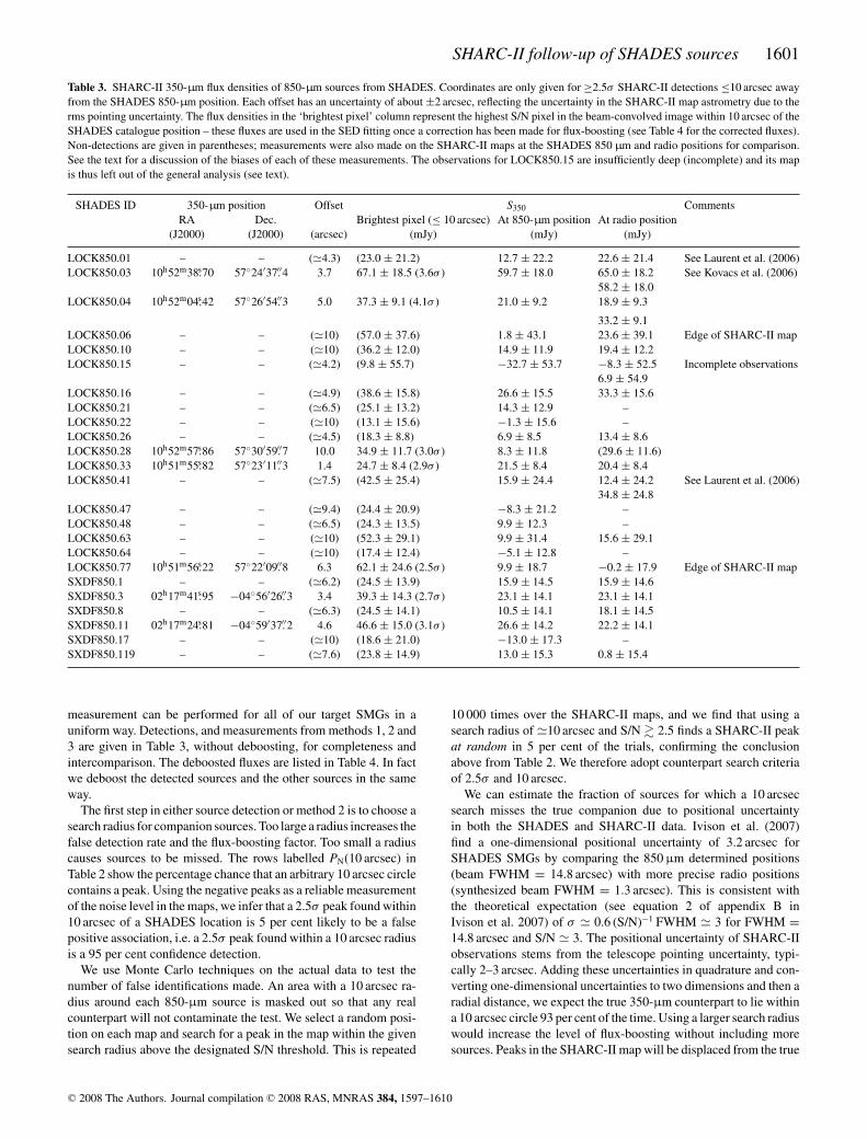
Table 3. SHARC-II 350-μm flux densities of 850-μm sources from SHADES. Coordinates are only given for ≥2.5σ SHARC-II detections ≤10 arcsec awayfrom the SHADES 850-μm position. Each offset has an uncertainty of about ±2 arcsec, reflecting the uncertainty in the SHARC-II map astrometry due to therms pointing uncertainty. The flux densities in the ‘brightest pixel’ column represent the highest S/N pixel in the beam-convolved image within 10 arcsec of theSHADES catalogue position – these fluxes are used in the SED fitting once a correction has been made for flux-boosting (see Table 4 for the corrected fluxes).Non-detections are given in parentheses; measurements were also made on the SHARC-II maps at the SHADES 850 μm and radio positions for comparison.See the text for a discussion of the biases of each of these measurements. The observations for LOCK850.15 are insufficiently deep (incomplete) and its mapis thus left out of the general analysis (see text).

SHADES ID 350-μm position Offset S350 CommentsRA Dec. Brightest pixel (≤ 10 arcsec) At 850-μm position At radio position

(J2000) (J2000) (arcsec) (mJy) (mJy) (mJy)

LOCK850.01 – – (�4.3) (23.0 ± 21.2) 12.7 ± 22.2 22.6 ± 21.4 See Laurent et al. (2006)LOCK850.03 10h52m38.s70 57◦24′37.′′4 3.7 67.1 ± 18.5 (3.6σ ) 59.7 ± 18.0 65.0 ± 18.2 See Kovacs et al. (2006)

58.2 ± 18.0LOCK850.04 10h52m04.s42 57◦26′54.′′3 5.0 37.3 ± 9.1 (4.1σ ) 21.0 ± 9.2 18.9 ± 9.3

33.2 ± 9.1LOCK850.06 – – (�10) (57.0 ± 37.6) 1.8 ± 43.1 23.6 ± 39.1 Edge of SHARC-II mapLOCK850.10 – – (�10) (36.2 ± 12.0) 14.9 ± 11.9 19.4 ± 12.2LOCK850.15 – – (�4.2) (9.8 ± 55.7) −32.7 ± 53.7 −8.3 ± 52.5 Incomplete observations

6.9 ± 54.9LOCK850.16 – – (�4.9) (38.6 ± 15.8) 26.6 ± 15.5 33.3 ± 15.6LOCK850.21 – – (�6.5) (25.1 ± 13.2) 14.3 ± 12.9 –LOCK850.22 – – (�10) (13.1 ± 15.6) −1.3 ± 15.6 –LOCK850.26 – – (�4.5) (18.3 ± 8.8) 6.9 ± 8.5 13.4 ± 8.6LOCK850.28 10h52m57.s86 57◦30′59.′′7 10.0 34.9 ± 11.7 (3.0σ ) 8.3 ± 11.8 (29.6 ± 11.6)LOCK850.33 10h51m55.s82 57◦23′11.′′3 1.4 24.7 ± 8.4 (2.9σ ) 21.5 ± 8.4 20.4 ± 8.4LOCK850.41 – – (�7.5) (42.5 ± 25.4) 15.9 ± 24.4 12.4 ± 24.2 See Laurent et al. (2006)

34.8 ± 24.8LOCK850.47 – – (�9.4) (24.4 ± 20.9) −8.3 ± 21.2 –LOCK850.48 – – (�6.5) (24.3 ± 13.5) 9.9 ± 12.3 –LOCK850.63 – – (�10) (52.3 ± 29.1) 9.9 ± 31.4 15.6 ± 29.1LOCK850.64 – – (�10) (17.4 ± 12.4) −5.1 ± 12.8 –LOCK850.77 10h51m56.s22 57◦22′09.′′8 6.3 62.1 ± 24.6 (2.5σ ) 9.9 ± 18.7 −0.2 ± 17.9 Edge of SHARC-II mapSXDF850.1 – – (�6.2) (24.5 ± 13.9) 15.9 ± 14.5 15.9 ± 14.6SXDF850.3 02h17m41.s95 −04◦56′26.′′3 3.4 39.3 ± 14.3 (2.7σ ) 23.1 ± 14.1 23.1 ± 14.1SXDF850.8 – – (�6.3) (24.5 ± 14.1) 10.5 ± 14.1 18.1 ± 14.5SXDF850.11 02h17m24.s81 −04◦59′37.′′2 4.6 46.6 ± 15.0 (3.1σ ) 26.6 ± 14.2 22.2 ± 14.1SXDF850.17 – – (�10) (18.6 ± 21.0) −13.0 ± 17.3 –SXDF850.119 – – (�7.6) (23.8 ± 14.9) 13.0 ± 15.3 0.8 ± 15.4

measurement can be performed for all of our target SMGs in auniform way. Detections, and measurements from methods 1, 2 and3 are given in Table 3, without deboosting, for completeness andintercomparison. The deboosted fluxes are listed in Table 4. In factwe deboost the detected sources and the other sources in the sameway.

The first step in either source detection or method 2 is to choose asearch radius for companion sources. Too large a radius increases thefalse detection rate and the flux-boosting factor. Too small a radiuscauses sources to be missed. The rows labelled PN(10 arcsec) inTable 2 show the percentage chance that an arbitrary 10 arcsec circlecontains a peak. Using the negative peaks as a reliable measurementof the noise level in the maps, we infer that a 2.5σ peak found within10 arcsec of a SHADES location is 5 per cent likely to be a falsepositive association, i.e. a 2.5σ peak found within a 10 arcsec radiusis a 95 per cent confidence detection.

We use Monte Carlo techniques on the actual data to test thenumber of false identifications made. An area with a 10 arcsec ra-dius around each 850-μm source is masked out so that any realcounterpart will not contaminate the test. We select a random posi-tion on each map and search for a peak in the map within the givensearch radius above the designated S/N threshold. This is repeated

10 000 times over the SHARC-II maps, and we find that using asearch radius of �10 arcsec and S/N � 2.5 finds a SHARC-II peakat random in 5 per cent of the trials, confirming the conclusionabove from Table 2. We therefore adopt counterpart search criteriaof 2.5σ and 10 arcsec.

We can estimate the fraction of sources for which a 10 arcsecsearch misses the true companion due to positional uncertaintyin both the SHADES and SHARC-II data. Ivison et al. (2007)find a one-dimensional positional uncertainty of 3.2 arcsec forSHADES SMGs by comparing the 850 μm determined positions(beam FWHM = 14.8 arcsec) with more precise radio positions(synthesized beam FWHM = 1.3 arcsec). This is consistent withthe theoretical expectation (see equation 2 of appendix B inIvison et al. 2007) of σ � 0.6 (S/N)−1 FWHM � 3 for FWHM =14.8 arcsec and S/N � 3. The positional uncertainty of SHARC-IIobservations stems from the telescope pointing uncertainty, typi-cally 2–3 arcsec. Adding these uncertainties in quadrature and con-verting one-dimensional uncertainties to two dimensions and then aradial distance, we expect the true 350-μm counterpart to lie withina 10 arcsec circle 93 per cent of the time. Using a larger search radiuswould increase the level of flux-boosting without including moresources. Peaks in the SHARC-II map will be displaced from the true



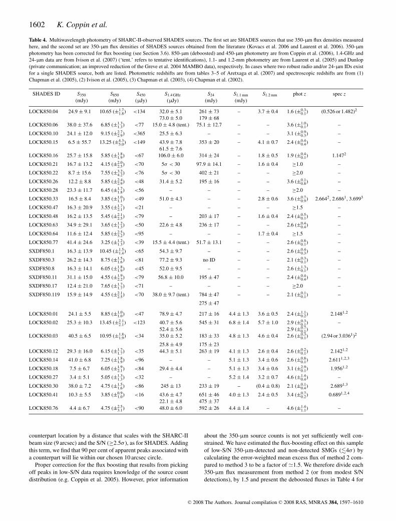
Table 4. Multiwavelength photometry of SHARC-II-observed SHADES sources. The first set are SHADES sources that use 350-μm flux densities measuredhere, and the second set are 350-μm flux densities of SHADES sources obtained from the literature (Kovacs et al. 2006 and Laurent et al. 2006). 350-μmphotometry has been corrected for flux boosting (see Section 3.6). 850-μm (deboosted) and 450-μm photometry are from Coppin et al. (2006), 1.4-GHz and24-μm data are from Ivison et al. (2007) (‘tent.’ refers to tentative identifications), 1.1- and 1.2-mm photometry are from Laurent et al. (2005) and Dunlop(private communication; an improved reduction of the Greve et al. 2004 MAMBO data), respectively. In cases where two robust radio and/or 24-μm IDs existfor a single SHADES source, both are listed. Photometric redshifts are from tables 3–5 of Aretxaga et al. (2007) and spectroscopic redshifts are from (1)Chapman et al. (2005), (2) Ivison et al. (2005), (3) Chapman et al. (2003), (4) Chapman et al. (2002).

SHADES ID S350 S850 S450 S1.4 GHz S24 S1.1 mm S1.2 mm phot z spec z(mJy) (mJy) (μJy) (μJy) (mJy) (mJy)

LOCK850.04 24.9 ± 9.1 10.65 (±1.71.8) <134 32.0 ± 5.1 261 ± 73 – 3.7 ± 0.4 1.6 (±0.3

0.1) (0.526 or 1.482)2

73.0 ± 5.0 179 ± 68LOCK850.06 38.0 ± 37.6 6.85 (±1.3

1.3) <77 15.0 ± 4.8 (tent.) 75.1 ± 12.7 – – 3.6 (±1.00.1) –

LOCK850.10 24.1 ± 12.0 9.15 (±2.72.9) <365 25.5 ± 6.3 – – – 3.1 (±0.9

0.3) –

LOCK850.15 6.5 ± 55.7 13.25 (±4.35.0) <149 43.9 ± 7.8 353 ± 20 – 4.1 ± 0.7 2.4 (±0.4

0.4) –61.5 ± 7.6

LOCK850.16 25.7 ± 15.8 5.85 (±1.81.9) <67 106.0 ± 6.0 314 ± 24 – 1.8 ± 0.5 1.9 (±0.4

0.1) 1.1472

LOCK850.21 16.7 ± 13.2 4.15 (±2.02.5) <70 5σ < 30 97.9 ± 14.1 – 1.6 ± 0.4 ≥1.0 –

LOCK850.22 8.7 ± 15.6 7.55 (±3.24.2) <76 5σ < 30 402 ± 21 – – ≥2.0 –

LOCK850.26 12.2 ± 8.8 5.85 (±2.42.9) <48 31.4 ± 5.2 195 ± 16 – – 3.6 (±0.1

0.8) –

LOCK850.28 23.3 ± 11.7 6.45 (±1.71.8) <56 – – – – ≥2.0 –

LOCK850.33 16.5 ± 8.4 3.85 (±1.01.1) <49 51.0 ± 4.3 – – 2.8 ± 0.6 3.6 (±0.7

0.9) 2.6642, 2.6861, 3.6993

LOCK850.47 16.3 ± 20.9 3.55 (±1.72.1) <21 – – – – ≥1.5 –

LOCK850.48 16.2 ± 13.5 5.45 (±2.12.5) <79 – 203 ± 17 – 1.6 ± 0.4 2.4 (±0.5

0.1) –

LOCK850.63 34.9 ± 29.1 3.65 (±1.21.3) <50 22.6 ± 4.8 236 ± 17 – – 2.6 (±0.4

0.4) –

LOCK850.64 11.6 ± 12.4 5.85 (±2.53.2) <95 – – – 1.7 ± 0.4 ≥1.5 –

LOCK850.77 41.4 ± 24.6 3.25 (±1.21.3) <39 15.5 ± 4.4 (tent.) 51.7 ± 13.1 – – 2.6 (±0.8

0.1) –

SXDF850.1 16.3 ± 13.9 10.45 (±1.51.4) <65 54.3 ± 9.7 – – – 2.6 (±0.4

0.3) –

SXDF850.3 26.2 ± 14.3 8.75 (±1.51.6) <81 77.2 ± 9.3 no ID – – 2.1 (±0.3

0.1) –

SXDF850.8 16.3 ± 14.1 6.05 (±1.81.9) <45 52.0 ± 9.5 – – – 2.6 (±1.3

0.1) –

SXDF850.11 31.1 ± 15.0 4.55 (±1.92.2) <79 56.8 ± 10.0 195 ± 47 – – 2.4 (±0.4

0.4) –

SXDF850.17 12.4 ± 21.0 7.65 (±1.71.7) <71 – – – – ≥2.0 –

SXDF850.119 15.9 ± 14.9 4.55 (±2.12.5) <70 38.0 ± 9.7 (tent.) 784 ± 47 – – 2.1 (±0.1

0.1) –

275 ± 47

LOCK850.01 24.1 ± 5.5 8.85 (±1.01.0) <47 78.9 ± 4.7 217 ± 16 4.4 ± 1.3 3.6 ± 0.5 2.4 (±1.1

0.2) 2.1481,2

LOCK850.02 25.3 ± 10.3 13.45 (±2.12.1) <123 40.7 ± 5.6 545 ± 31 6.8 ± 1.4 5.7 ± 1.0 2.9 (±0.3

0.1) –52.4 ± 5.6 2.9 (±0.7

0.1)LOCK850.03 40.5 ± 6.5 10.95 (±1.8

1.9) <34 35.0 ± 5.2 183 ± 33 4.8 ± 1.3 4.6 ± 0.4 2.6 (±0.30.1) (2.94 or 3.0361)2

25.8 ± 4.9 175 ± 23LOCK850.12 29.3 ± 16.0 6.15 (±1.7

1.7) <35 44.3 ± 5.1 263 ± 19 4.1 ± 1.3 2.6 ± 0.4 2.6 (±0.20.1) 2.1421,2

LOCK850.14 41.0 ± 6.8 7.25 (±1.81.9) <96 – – 5.1 ± 1.3 3.4 ± 0.6 2.6 (±0.8

0.1) 2.6111,2,3

LOCK850.18 7.5 ± 6.7 6.05 (±1.92.1) <84 29.4 ± 4.4 – 5.1 ± 1.3 3.4 ± 0.6 3.1 (±2.9

0.1) 1.9561,2

LOCK850.27 3.4 ± 5.1 5.05 (±1.31.3) <32 – – 5.2 ± 1.4 3.2 ± 0.7 4.6 (±1.4

0.4) –

LOCK850.30 38.0 ± 7.2 4.75 (±1.51.6) <86 245 ± 13 233 ± 19 – (0.4 ± 0.8) 2.1 (±0.1

0.4) 2.6891,3

LOCK850.41 10.3 ± 5.5 3.85 (±0.91.0) <16 43.6 ± 4.7 651 ± 46 4.0 ± 1.3 2.4 ± 0.5 3.4 (±0.7

0.2) 0.6891,2,4

22.1 ± 4.8 475 ± 37LOCK850.76 4.4 ± 6.7 4.75 (±2.5

3.1) <90 48.0 ± 6.0 592 ± 26 4.4 ± 1.4 – 4.6 (±1.41.1) –

counterpart location by a distance that scales with the SHARC-IIbeam size (9 arcsec) and the S/N (≥2.5σ ), as for SHADES. Addingthis term, we find that 90 per cent of apparent peaks associated witha counterpart will lie within our chosen 10 arcsec circle.

Proper correction for the flux boosting that results from pickingoff peaks in low-S/N data requires knowledge of the source countdistribution (e.g. Coppin et al. 2005). However, prior information

about the 350-μm source counts is not yet sufficiently well con-strained. We have estimated the flux-boosting effect on this sampleof low-S/N 350-μm-detected and non-detected SMGs (�4σ ) bycalculating the error-weighted mean excess flux of method 2 com-pared to method 3 to be a factor of �1.5. We therefore divide each350-μm flux measurement from method 2 (or from modest S/Ndetections), by 1.5 and present the deboosted fluxes in Table 4 for



use in fitting SEDs. For the highest S/N 350-μm-detected SMGs(�4.5σ ; Kovacs et al. 2006), flux-boosting effects are negligibleand so we do not correct these fluxes.

3.4 Discussion of other 350-μm photometry of 850-μm

SHADES sources

The 350-μm flux densities have been constrained for 25 per centof the SHADES 850-μm sources, with the current work provid-ing 21/31 of the SHADES 350-μm flux density constraints. Com-plementary SHARC-II observations of SMGs including severalSHADES sources have been performed by Laurent et al. (2006)and Kovacs et al. (2006). Since we include their photometry in theSED fits of seven SHADES sources, it is worth describing howfluxes are measured by these groups.

Kovacs et al. (2006) conducted follow-up observations ofbright (>5 mJy) radio-identified SCUBA sources with opticalspectroscopic redshifts, including LOCK850.3, LOCK850.14,LOCK850.18 and LOCK850.30. They detected 12/15 of their sam-ple with a mean S/N � 4.5 for the detections.

Laurent et al. (2006) performed follow-up observationsof 17 Bolocam 1.1-mm-selected source candidates in theLH with SHARC-II. Of the 17, 10 are detected, in-cluding LOCK850.1, LOCK850.2, LOCK850.3, LOCK850.12,LOCK850.14, LOCK850.41, LOCK850.27 and LOCK850.763 (seeLaurent et al. 2005 for counterpart identifications4).

Kovacs et al. (2006) and Laurent et al. (2006) quote as a fluxthe peak flux density in a specified search radius around their targetsource position, which is taken from either radio or mm data. Theydo not deboost these fluxes, but their observations are at lower noiselevels so this step is less important.

Three SHADES sources that we observe in this programme,LOCK850.1, LOCK850.3 and LOCK850.41 have also been ob-served by Kovacs et al. (2006) and Laurent et al. (2006). Becausetheir observations are at lower noise we use their fluxes in Table 4and in subsequent analysis.

3.5 Formally detected 350-μm counterparts

In the analysis section of this paper we use our best estimates of the350-μm flux of each source as photometric constraints. However,for comparison to blank field surveys it is useful to consider howmany of the sources are seen at a high enough S/N that they wouldbe counted as detections.

We have identified seven 350-μm counterparts of 850-μmsources, as presented in Table 3. The positional offsets of the detec-tions from the SHADES positions are consistent with the positionaldistribution discussed above; 5/7 (71 per cent) of the detectionslie within 5 arcsec. No trend is seen of decreasing positional offsetwith increasing S/N ratio of the seven associations, but this is notsurprising given the low number statistics and the small dynamicrange in S/N.

3 LOCK850.3 and LOCK850.14 are detected by Kovacs et al. (2006) butalso discussed by Laurent et al. (2006).4 LOCK850.27 and LOCK850.76 were not previously associated with Bolo-cam sources, since they are new SHADES detections. LOCK850.27 andLOCK850.76 lie 4.8 and 10.6 arcsec away from two Bolocam sources, andso two new SCUBA/Bolocam associations are claimed here.

It is striking that the number of detected counterparts to SHADESsources exactly matches the excess of positive peaks over noise (ornegative peaks) in the full mapped area, as listed in Table 2.

As we did with the number of peaks, we can use the correspondingcomposite negative catalogue to test if real associations are beingfound or just noisy peaks in the 350-μm maps. Counterparts to850-μm sources are searched for in an inverted map in the sameway, using an S/N threshold of 2.5 and search radius of 10 arcsecand no ‘negative’ counterparts are identified. This result reassuresus that the 350-/850-μm associations are likely to be real.

3.6 350-μm flux density constraints of SMGs not individually

detected by SHARC-II

Any of the following mechanisms might cause an SMG not to bedetected at 350 μm. (1) The 850-μm source could be intrinsicallyless luminous, colder and/or have a different SED shape than thestrongly detected sources. (2) The SMG could lie at a redshift inexcess of about 3, this being more likely if there is also no radiocounterpart, since the existing radio data are sufficiently deep toobtain a large fraction of counterparts for SMGs only for z � 3 (seeIvison et al. 2005). Above z ∼ 3, the 350-μm band is sampling theWien side of the SED and suffers from cosmological dimming with-out the benefit of the negative K-correction. (3) The SMG could bespurious, although the false positive rate in the SHADES catalogueis believed to be very low. The catalogue was carefully constructedfrom a comparison of multiple data reductions in order to minimizefalse detections (see Coppin et al. 2006).

We rely on the photometric fluxes even for the 16 sourceswhich are not detected at high significance. Therefore we haveperformed a stacking analysis to determine if a significantly posi-tive 350-μm flux density is associated with those sources. 350-μmflux densities and errors are measured on the SHARC-II mapsat the radio position for 11 of these 16 sources which have aradio counterpart and we find a mean flux of 16.7 ± 4.8 mJy.This is our least biased flux estimator, and the agreement withour listed deboosted fluxes is very encouraging. The weightedmean deboosted flux for all 16 of these low significance sources is16.6 ± 3.8 mJy.

3.7 Serendipitous 350-μm blank-field SMGs

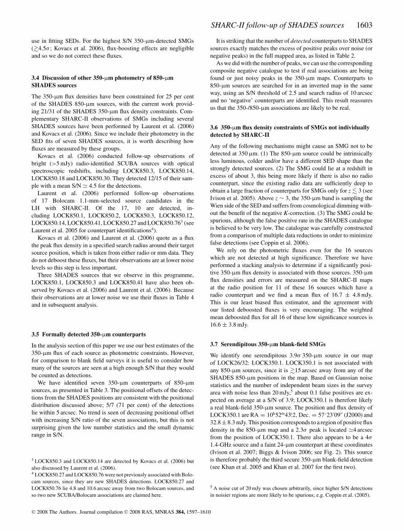
We identify one serendipitous 3.9σ 350-μm source in our mapof LOCK26/32: LOCK350.1. LOCK350.1 is not associated withany 850-μm sources, since it is �15 arcsec away from any of theSHADES 850-μm positions in the map. Based on Gaussian noisestatistics and the number of independent beam sizes in the surveyarea with noise less than 20 mJy,5 about 0.1 false positives are ex-pected on average at a S/N of 3.9; LOCK350.1 is therefore likelya real blank-field 350-μm source. The position and flux density ofLOCK350.1 are RA = 10h52m43.s2, Dec. = 57◦23′09′′ (J2000) and32.8 ± 8.3 mJy. This position corresponds to a region of positive fluxdensity in the 850-μm map and a 2.3σ peak is located �4 arcsecfrom the position of LOCK350.1. There also appears to be a 4σ

1.4-GHz source and a faint 24-μm counterpart at these coordinates(Ivison et al. 2007; Biggs & Ivison 2006; see Fig. 2). This sourceis therefore probably the third secure 350-μm blank-field detection(see Khan et al. 2005 and Khan et al. 2007 for the first two).

5 A noise cut of 20 mJy was chosen arbitrarily, since higher S/N detectionsin noisier regions are more likely to be spurious; e.g. Coppin et al. (2005).



Figure 2. A multiwavelength view of LOCK350.1, a 3.9σ 350-μm blank-field source detected at RA = 10h52m43.s2, Dec. = 57◦23′9′′ (J2000). The30 × 30 arcsec2 images are centred on the position of LOCK350.1. Left-hand panel: High-resolution (1.3 arcsec) 1.4-GHz contours (−3, 3, 4, . . . ,10,20, . . . ,100 ×σ ) from Biggs & Ivison (2006) overlaid on grey-scale archivalR-band optical data. Right-hand panel: Low-resolution (4.2 arcsec) 1.4-GHzcontours (−3, 3, 4, . . . ,10, 20, . . . ,100 ×σ ) from Biggs & Ivison (2006)overlaid on grey-scale 24-μm data from Ivison et al. (2007).

4 A NA LY SIS A N D RESULTS

4.1 Constraints on the 350-μm source counts

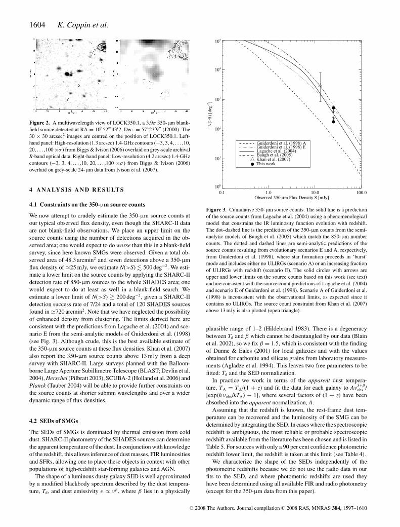
We now attempt to crudely estimate the 350-μm source counts atour typical observed flux density, even though the SHARC-II dataare not blank-field observations. We place an upper limit on thesource counts using the number of detections acquired in the ob-served area; one would expect to do worse than this in a blank-fieldsurvey, since here known SMGs were observed. Given a total ob-served area of 48.3 arcmin2 and seven detections above a 350-μmflux density of �25 mJy, we estimate N(>S) � 500 deg−2. We esti-mate a lower limit on the source counts by applying the SHARC-IIdetection rate of 850-μm sources to the whole SHADES area; onewould expect to do at least as well in a blank-field search. Weestimate a lower limit of N(>S) � 200 deg−2, given a SHARC-IIdetection success rate of 7/24 and a total of 120 SHADES sourcesfound in �720 arcmin2. Note that we have neglected the possibilityof enhanced density from clustering. The limits derived here areconsistent with the predictions from Lagache et al. (2004) and sce-nario E from the semi-analytic models of Guiderdoni et al. (1998)(see Fig. 3). Although crude, this is the best available estimate ofthe 350-μm source counts at these flux densities. Khan et al. (2007)also report the 350-μm source counts above 13 mJy from a deepsurvey with SHARC-II. Large surveys planned with the Balloon-borne Large Aperture Subillimetre Telescope (BLAST; Devlin et al.2004), Herschel (Pilbratt 2003), SCUBA-2 (Holland et al. 2006) andPlanck (Tauber 2004) will be able to provide further constraints onthe source counts at shorter submm wavelengths and over a widerdynamic range of flux densities.

4.2 SEDs of SMGs

The SEDs of SMGs is dominated by thermal emission from colddust. SHARC-II photometry of the SHADES sources can determinethe apparent temperature of the dust. In conjunction with knowledgeof the redshift, this allows inference of dust masses, FIR luminositiesand SFRs, allowing one to place these objects in context with otherpopulations of high-redshift star-forming galaxies and AGN.

The shape of a luminous dusty galaxy SED is well approximatedby a modified blackbody spectrum described by the dust tempera-ture, Td, and dust emissivity ε ∝ νβ , where β lies in a physically

0.1 1.0 10.0 100.0Observed 350 μm Flux Density S [mJy]

100

101

102

103

104

105

N(>

S)

[deg

-2]

Guiderdoni et al. (1998) AGuiderdoni et al. (1998) ELagache et al. (2004)Baugh et al. (2005)Khan et al. (2007)This work

Figure 3. Cumulative 350-μm source counts. The solid line is a predictionof the source counts from Lagache et al. (2004) using a phenomenologicalmodel that constrains the IR luminosity function evolution with redshift.The dot–dashed line is the prediction of the 350-μm counts from the semi-analytic models of Baugh et al. (2005) which match the 850-μm numbercounts. The dotted and dashed lines are semi-analytic predictions of thesource counts resulting from evolutionary scenarios E and A, respectively,from Guiderdoni et al. (1998), where star formation proceeds in ‘burst’mode and includes either no ULIRGs (scenario A) or an increasing fractionof ULIRGs with redshift (scenario E). The solid circles with arrows areupper and lower limits on the source counts based on this work (see text)and are consistent with the source count predictions of Lagache et al. (2004)and scenario E of Guiderdoni et al. (1998). Scenario A of Guiderdoni et al.(1998) is inconsistent with the observational limits, as expected since itcontains no ULIRGs. The source count constraint from Khan et al. (2007)above 13 mJy is also plotted (open triangle).

plausible range of 1–2 (Hildebrand 1983). There is a degeneracybetween Td and β which cannot be disentangled by our data (Blainet al. 2002), so we fix β = 1.5, which is consistent with the findingof Dunne & Eales (2001) for local galaxies and with the valuesobtained for carbonite and silicate grains from laboratory measure-ments (Agladze et al. 1994). This leaves two free parameters to befitted: Td and the SED normalization.

In practice we work in terms of the apparent dust tempera-ture, TA = Td/(1 + z) and fit the data for each galaxy to Aν

3+β

obs /[exp(h νobs/kTA) − 1], where several factors of (1 + z) have beenabsorbed into the apparent normalization, A.

Assuming that the redshift is known, the rest-frame dust tem-perature can be recovered and the luminosity of the SMG can bedetermined by integrating the SED. In cases where the spectroscopicredshift is ambiguous, the most reliable or probable spectroscopicredshift available from the literature has been chosen and is listed inTable 5. For sources with only a 90 per cent confidence photometricredshift lower limit, the redshift is taken at this limit (see Table 4).

We characterize the shape of the SEDs independently of thephotometric redshifts because we do not use the radio data in ourfits to the SED, and where photometric redshifts are used theyhave been determined using all available FIR and radio photometry(except for the 350-μm data from this paper).



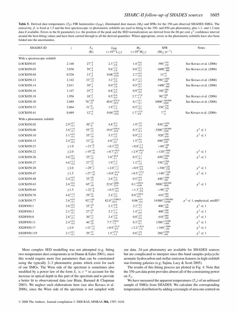
Table 5. Derived dust temperatures (Td), FIR luminosities (LFIR), illuminated dust masses (Md) and SFRs for the 350-μm observed SHADES SMGs. Theemissivity, β, is fixed at 1.5 and the best spectroscopic or photometric redshifts are used in fitting to the 350- and 850-μm photometry, plus 1.1- and 1.2-mmdata if available. Errors in the fit parameters (i.e. the position of the peak and the SED normalization) are derived from the 68 per cent χ2 confidence intervalaround the best-fitting values and have been carried through to all the derived quantities. Where appropriate, errors in the photometric redshifts have also beenfolded into the uncertainties.

SHADES ID z Td LFIR Md SFR Notes(K) (×1012 L�) (×109 M�) (M� yr−1)

With a spectroscopic redshift

LOCK850.01 2.148 27+4−3 2.3+1.0

−0.8 1.4+0.6−0.3 390+170

−130 See Kovacs et al. (2006)

LOCK850.03 3.036 39+4−4 9.6+3.5

−2.8 0.8+0.2−0.2 1600+600


LOCK850.04 0.526 13+2−2 0.08+0.03

−0.03 2.7+0.9−0.6 13+6

−4

LOCK850.12 2.142 33+14−12 3.2+8.2

−2.6 0.7+1.4−0.3 550+1400


LOCK850.14 2.611 39+7−5 8.0+4.6

−2.8 0.5+0.2−0.1 1400+790


LOCK850.16 1.147 25+9−7 0.8+1.6

−0.5 0.9+0.8−0.4 140+280

−90

LOCK850.18 1.956 18+5−7 0.5+0.6

−0.4 2.7+17.0−1.3 90+100


LOCK850.30 2.689 76+103−21 40.0+932.0

−26.0 0.1+0.1−0.1 6900+160 000


LOCK850.33 2.664 31+8−13 1.9+2.1

−1.5 0.5+2.1−0.2 330+370

−270

LOCK850.41 0.689 12+4−6 0.04+0.05

−0.03 1.7+12.0−0.8 7+9


With a photometric redshift

LOCK850.02 2.9+0.7−0.1 30+12

−8 4.8+8.3−2.9 1.9+2.0

−1.0 830+1430−490

LOCK850.06 3.6+1.0−0.1 55+51

−33 19.0+930.0−19.0 0.3+2.5

−0.2 3300+160 000−3200 χ2 1

LOCK850.10 3.1+0.9−0.3 35+17

−10 5.3+4.5−3.5 0.9+1.2

−0.3 920+780−610 χ2 1

LOCK850.15 2.4+0.4−0.4 33+17

−29 4.0+37.0−3.6 1.5+9.0

−1.0 690+6400−630

LOCK850.21 ≥1.0 >21+8−7 >0.3+0.6

−0.2 >0.8+1.5−0.4 >60+100

−40

LOCK850.22 ≥2.0 >19+10−10 >0.7+18.0

−0.7 >2.9+49.0−1.8 >120+3000

−110 χ2 1

LOCK850.26 3.6+0.1−0.8 35+11

−15 3.8+30.0−3.1 0.5+1.7

−0.3 650+5200−540 χ2 1

LOCK850.27 4.6+1.4−0.4 27+22

−11 1.9+1.2−1.2 1.2+9.1

−1.0 330+1200−210

LOCK850.28 ≥2.0 >29+7−7 >2.0+1.3

−1.3 >0.9+0.9−0.9 >340+220

−220 χ2 1

LOCK850.47 ≥1.5 >27+19−19 >0.8+41.0

−0.8 >0.5+37.0−0.3 >140+7100

−140 χ2 1

LOCK850.48 2.4+0.5−0.1 35+20

−12 2.6+9.4−2.0 0.5+0.8

−0.3 440+1600−340

LOCK850.63 2.6+0.4−0.4 65+71

−59 22.0+2600.−22.0 0.1+850.0

−0.08 3800+460 000−3800 χ2 1

LOCK850.64 ≥1.5 >22+8−8 >0.5+0.9

−0.4 >1.3+2.8−0.6 >90+150

−70

LOCK850.76 4.6+1.4−1.1 29+21

−19 2.4+2.1−2.0 0.9+100.0

−0.4 410+360−350

LOCK850.77 2.6+0.8−0.1 92+140

−75 82.0+13 000.0−82.0 0.06+0.6

−0.4 14 000+2300 000−14 000 χ2 1, unphysical, misID?

SXDF850.1 2.6+0.4−0.3 25+10

−8 2.3+0.8−1.8 2.2+4.4

−1.2 400+130−300 χ2 1

SXDF850.3 2.1+0.3−0.1 27+10

−8 2.3+1.7−1.6 1.4+1.5

−0.6 400+300−270 χ2 1

SXDF850.8 2.6+1.3−0.1 30+11

−11 2.4+3.9−2.0 0.8+2.0

−0.4 410+680−340 χ2 1

SXDF850.11 2.4+0.4−0.4 46+29

−24 7.7+190.0−7.3 0.3+0.9

−0.1 1300+32 000−1300 χ2 1

SXDF850.17 ≥2.0 >21+11−11 >0.9+23.0

−0.9 >2.2+36.0−1.4 >160+3900

−150 χ2 1

SXDF850.119 2.1+0.1−0.1 29+15

−14 1.5+27.0−1.4 0.6+2.8

−0.3 260+4700−240 χ2 1

More complex SED modelling was not attempted (e.g. fittingtwo-temperature dust components as in Dunne & Eales 2001), sincethis would require more free parameters than can be constrainedusing the typically 2–3 photometric points which exist for eachof our SMGs. The Wien side of the spectrum is sometimes alsomodified by a power law of the form Sν ∝ ν−α to account for theincrease in optical depth in this part of the spectrum and to providea better fit to observational data (see Blain, Barnard & Chapman2003). We neglect such elaborations here (see also Kovacs et al.2006), since the Wien side of the spectrum is not sampled with

our data. 24-μm photometry are available for SHADES sourcesbut are complicated to interpret since this band samples polycyclicaromatic hydrocarbon and stellar emission features in high-redshiftstar-forming galaxies (e.g. Sajina, Lacy & Scott 2005).

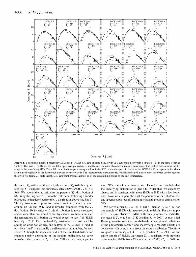
The results of this fitting process are plotted in Fig. 4. Note thatthe 350-μm data point provides almost all of the constraining poweron TA.

We have measured the apparent temperatures (TA) of an unbiasedsample of SMGs from SHADES. We calculate the correspondingtemperature distribution by adding a rectangle of area one centred on



1

10

100

LOCK850.1z = 2.15T

d= 27

1

LOCK850.3z = 3.04T

d= 39

1

LOCK850.4z = 0.53T

d= 13

1

LOCK850.12z = 2.14T

d= 33

1

LOCK850.14z = 2.61T

d= 39

1

LOCK850.16z = 1.15T

d= 25

1

10

100

LOCK850.18z = 1.96T

d= 18

1

LOCK850.30z = 2.69T

d= 76

1

LOCK850.33z = 2.66T

d= 31

1

LOCK850.41z = 0.69T

d= 12

1

LOCK850.2z = 2.90T

d= 30

1

LOCK850.06z = 3.60T

d= 55

1

10

100

LOCK850.10z = 3.10T

d= 34

1

LOCK850.15z = 2.40T

d= 33

1

LOCK850.21z = 1.00T

d= 21

1

LOCK850.22z = 2.00T

d= 19

1

LOCK850.26z = 3.60T

d= 35

1

LOCK850.27z = 4.60T

d= 27

1

10

100

LOCK850.28z = 2.00T

d= 29

1

LOCK850.47z = 1.50T

d= 27

1

LOCK850.48z = 2.40T

d= 35

1

LOCK850.63z = 2.60T

d= 65

1

LOCK850.64z = 1.50T

d= 22

1

LOCK850.76z = 4.60T

d= 29

1

10

100

LOCK850.77z = 2.60T

d= 92

100 10001

SXDF850.1z = 2.60T

d= 25

100 10001

SXDF850.3z = 2.10T

d= 27

100 10001

SXDF850.8z = 2.60T

d= 30

100 10001

SXDF850.11z = 2.40T

d= 46

100 10001

SXDF850.17z = 2.00T

d= 21

100 10001

10

100

SXDF850.119z = 2.10T

d= 29

Observed λ [ μm]

Obs

erve

d S

ν [m

Jy]

Figure 4. Best-fitting modified blackbody SEDs for SHADES 850-μm-selected SMGs with 350-μm photometry with β fixed to 1.5, in the same order asTable 5. The first 10 SEDs use the available spectroscopic redshifts, and the rest use only photometric redshift constraints. The dashed curves show the 1σ

range in the best-fitting SED. The solid circles indicate photometry used to fit the SED, while the open circles show the SCUBA 450 μm upper limits whichare not used explicitly in the fits (though they are never violated). The spectroscopic or photometric redshifts indicated in each panel have been used to recoverthe given rest-frame Td. Note that the 350-μm point provides almost all of the constraining power on the dust temperature.

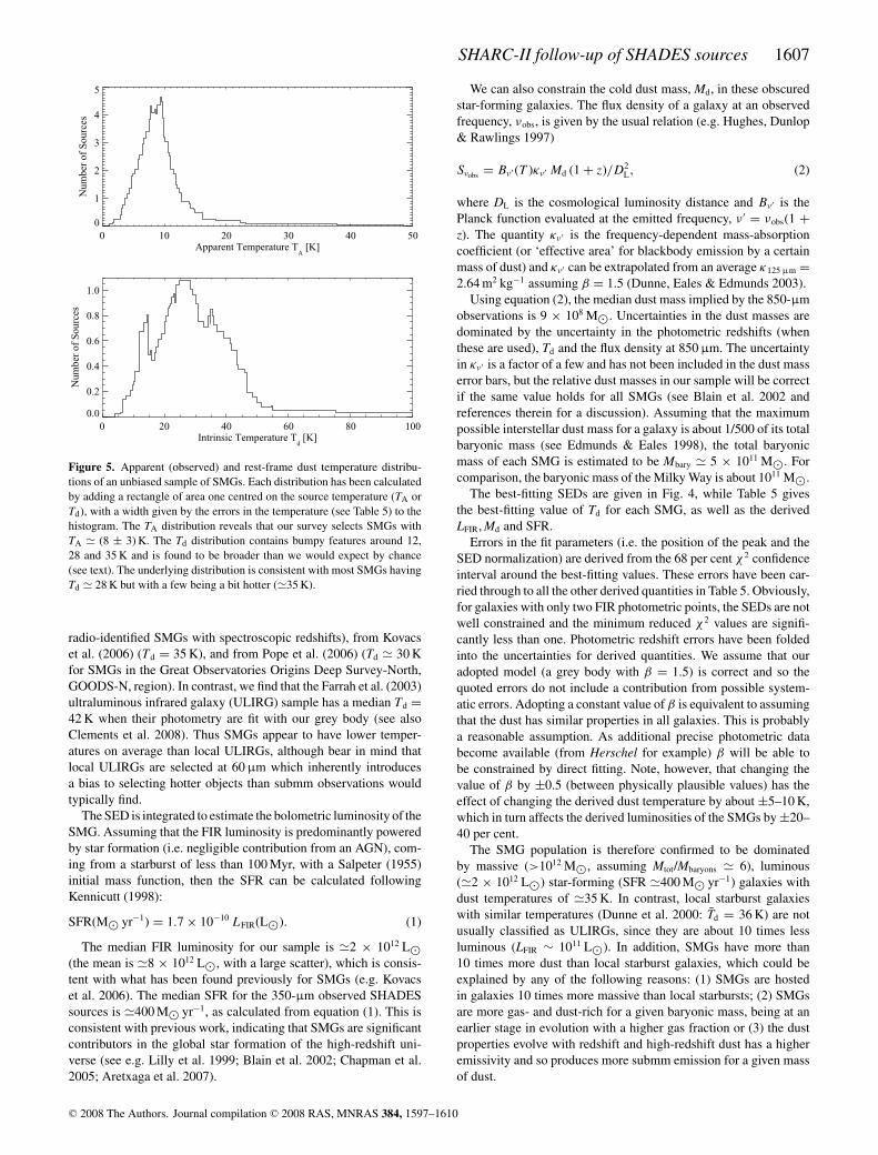
the source TA, with a width given by the errors in TA to the histogram(see Fig. 5). It appears that our survey selects SMGs with TA � (8 ±3) K. We recover the intrinsic dust temperature (Td) distribution ofSMGs by shifting each SED into the rest frame, following a similarprocedure to that described for the TA distribution above (see Fig. 5).The Td distribution appears to contain structure (‘bumps’ centredaround 12, 28 and 35 K) and is broader compared with the TA

distribution. To investigate if this distribution is more structuredand/or wider than we would expect by chance, we have simulatedthe temperature distribution we would expect to see if all SMGshave Td = 28 K. The simulated Td distribution is constructed byadding an error box of area one centred on Td = 28 K + rand ×σ , where ‘rand’ is a normally distributed random number, for eachsource. Although the shape and width of the simulated distributionchanges notably depending on the random realization, we neverreproduce the ‘bumps’ at Td � 12 or 35 K and we always predict

more SMGs at a few K than we see. Therefore we conclude thatthe underlying distribution is just a bit wider than we expect bychance and is consistent with most SMGs at 28 K with a few hotterones. Now we compare the dust temperatures of our photometricand spectroscopic redshift subsamples and to previous estimates forSMGs.

We derive a mean Td = (31 ± 18) K (median Td = 31 K) forour sample of SMGs with spectroscopic redshifts. For the sampleof 21 350-μm observed SMGs with only photometric redshifts,the mean is Td = (35 ± 17) K (median Td = 29 K). A two-sidedKolmogorov–Smirnov test reveals that the temperature distributionsof the photometric redshift and spectroscopic redshift subsets areconsistent with being drawn from the same distribution. Thereforewe quote a mean Td = (34 ± 17) K (median Td = 29 K) for ourentire sample of SMGs. Our mean Td is consistent with previousestimates for SMGs from Chapman et al. (2005) (Td = 36 K for



0 10 20 30 40 50Apparent Temperature T

A [K]

0

1

2

3

4

5N

umbe

r of

Sou

rces

0 20 40 60 80 100Intrinsic Temperature T

d [K]

0.0

0.2

0.4

0.6

0.8

1.0

Num

ber

of S

ourc

es

Figure 5. Apparent (observed) and rest-frame dust temperature distribu-tions of an unbiased sample of SMGs. Each distribution has been calculatedby adding a rectangle of area one centred on the source temperature (TA orTd), with a width given by the errors in the temperature (see Table 5) to thehistogram. The TA distribution reveals that our survey selects SMGs withTA � (8 ± 3) K. The Td distribution contains bumpy features around 12,28 and 35 K and is found to be broader than we would expect by chance(see text). The underlying distribution is consistent with most SMGs havingTd � 28 K but with a few being a bit hotter (�35 K).

radio-identified SMGs with spectroscopic redshifts), from Kovacset al. (2006) (Td = 35 K), and from Pope et al. (2006) (Td � 30 Kfor SMGs in the Great Observatories Origins Deep Survey-North,GOODS-N, region). In contrast, we find that the Farrah et al. (2003)ultraluminous infrared galaxy (ULIRG) sample has a median Td =42 K when their photometry are fit with our grey body (see alsoClements et al. 2008). Thus SMGs appear to have lower temper-atures on average than local ULIRGs, although bear in mind thatlocal ULIRGs are selected at 60 μm which inherently introducesa bias to selecting hotter objects than submm observations wouldtypically find.

The SED is integrated to estimate the bolometric luminosity of theSMG. Assuming that the FIR luminosity is predominantly poweredby star formation (i.e. negligible contribution from an AGN), com-ing from a starburst of less than 100 Myr, with a Salpeter (1955)initial mass function, then the SFR can be calculated followingKennicutt (1998):

SFR(M� yr−1) = 1.7 × 10−10 LFIR(L�). (1)

The median FIR luminosity for our sample is �2 × 1012 L�(the mean is �8 × 1012 L�, with a large scatter), which is consis-tent with what has been found previously for SMGs (e.g. Kovacset al. 2006). The median SFR for the 350-μm observed SHADESsources is �400 M� yr−1, as calculated from equation (1). This isconsistent with previous work, indicating that SMGs are significantcontributors in the global star formation of the high-redshift uni-verse (see e.g. Lilly et al. 1999; Blain et al. 2002; Chapman et al.2005; Aretxaga et al. 2007).

We can also constrain the cold dust mass, Md, in these obscuredstar-forming galaxies. The flux density of a galaxy at an observedfrequency, νobs, is given by the usual relation (e.g. Hughes, Dunlop& Rawlings 1997)

Sνobs = Bν′ (T )κν′ Md (1 + z)/D2L, (2)

where DL is the cosmological luminosity distance and Bν′ is thePlanck function evaluated at the emitted frequency, ν ′ = νobs(1 +z). The quantity κν′ is the frequency-dependent mass-absorptioncoefficient (or ‘effective area’ for blackbody emission by a certainmass of dust) and κν′ can be extrapolated from an average κ125 μm =2.64 m2 kg−1 assuming β = 1.5 (Dunne, Eales & Edmunds 2003).

Using equation (2), the median dust mass implied by the 850-μmobservations is 9 × 108 M�. Uncertainties in the dust masses aredominated by the uncertainty in the photometric redshifts (whenthese are used), Td and the flux density at 850 μm. The uncertaintyin κν′ is a factor of a few and has not been included in the dust masserror bars, but the relative dust masses in our sample will be correctif the same value holds for all SMGs (see Blain et al. 2002 andreferences therein for a discussion). Assuming that the maximumpossible interstellar dust mass for a galaxy is about 1/500 of its totalbaryonic mass (see Edmunds & Eales 1998), the total baryonicmass of each SMG is estimated to be Mbary � 5 × 1011 M�. Forcomparison, the baryonic mass of the Milky Way is about 1011 M�.

The best-fitting SEDs are given in Fig. 4, while Table 5 givesthe best-fitting value of Td for each SMG, as well as the derivedLFIR, Md and SFR.

Errors in the fit parameters (i.e. the position of the peak and theSED normalization) are derived from the 68 per cent χ 2 confidenceinterval around the best-fitting values. These errors have been car-ried through to all the other derived quantities in Table 5. Obviously,for galaxies with only two FIR photometric points, the SEDs are notwell constrained and the minimum reduced χ 2 values are signifi-cantly less than one. Photometric redshift errors have been foldedinto the uncertainties for derived quantities. We assume that ouradopted model (a grey body with β = 1.5) is correct and so thequoted errors do not include a contribution from possible system-atic errors. Adopting a constant value of β is equivalent to assumingthat the dust has similar properties in all galaxies. This is probablya reasonable assumption. As additional precise photometric databecome available (from Herschel for example) β will be able tobe constrained by direct fitting. Note, however, that changing thevalue of β by ±0.5 (between physically plausible values) has theeffect of changing the derived dust temperature by about ±5–10 K,which in turn affects the derived luminosities of the SMGs by ±20–40 per cent.

The SMG population is therefore confirmed to be dominatedby massive (>1012 M�, assuming Mtot/Mbaryons � 6), luminous(�2 × 1012 L�) star-forming (SFR �400 M� yr−1) galaxies withdust temperatures of �35 K. In contrast, local starburst galaxieswith similar temperatures (Dunne et al. 2000: Td = 36 K) are notusually classified as ULIRGs, since they are about 10 times lessluminous (LFIR ∼ 1011 L�). In addition, SMGs have more than10 times more dust than local starburst galaxies, which could beexplained by any of the following reasons: (1) SMGs are hostedin galaxies 10 times more massive than local starbursts; (2) SMGsare more gas- and dust-rich for a given baryonic mass, being at anearlier stage in evolution with a higher gas fraction or (3) the dustproperties evolve with redshift and high-redshift dust has a higheremissivity and so produces more submm emission for a given massof dust.



5 D ISCUSSION

5.1 Trends in the data and consideration of selection effects

We first consider selection effects in our data before looking fortrends in the derived properties. It is not surprising that the S350/S850

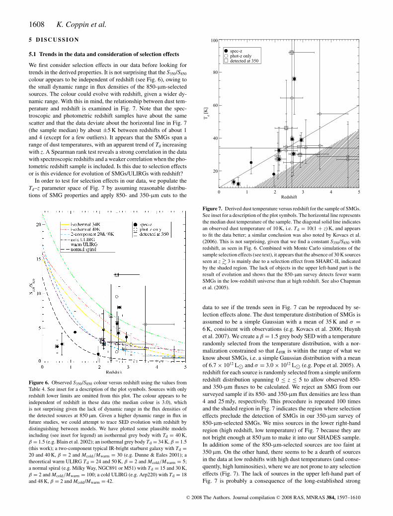
colour appears to be independent of redshift (see Fig. 6), owing tothe small dynamic range in flux densities of the 850-μm-selectedsources. The colour could evolve with redshift, given a wider dy-namic range. With this in mind, the relationship between dust tem-perature and redshift is examined in Fig. 7. Note that the spec-troscopic and photometric redshift samples have about the samescatter and that the data deviate about the horizontal line in Fig. 7(the sample median) by about ±5 K between redshifts of about 1and 4 (except for a few outliers). It appears that the SMGs span arange of dust temperatures, with an apparent trend of Td increasingwith z. A Spearman rank test reveals a strong correlation in the datawith spectroscopic redshifts and a weaker correlation when the pho-tometric redshift sample is included. Is this due to selection effectsor is this evidence for evolution of SMGs/ULIRGs with redshift?

In order to test for selection effects in our data, we populate theTd–z parameter space of Fig. 7 by assuming reasonable distribu-tions of SMG properties and apply 850- and 350-μm cuts to the

Figure 6. Observed S350/S850 colour versus redshift using the values fromTable 4. See inset for a description of the plot symbols. Sources with onlyredshift lower limits are omitted from this plot. The colour appears to beindependent of redshift in these data (the median colour is 3.0), whichis not surprising given the lack of dynamic range in the flux densities ofthe detected sources at 850 μm. Given a higher dynamic range in flux infuture studies, we could attempt to trace SED evolution with redshift bydistinguishing between models. We have plotted some plausible modelsincluding (see inset for legend) an isothermal grey body with Td = 40 K,β = 1.5 (e.g. Blain et al. 2002); an isothermal grey body Td = 34 K, β = 1.5(this work); a two-component typical IR-bright starburst galaxy with Td =20 and 40 K, β = 2 and Mcold/Mwarm = 30 (e.g. Dunne & Eales 2001); atheoretical warm ULIRG Td = 24 and 50 K, β = 2 and Mcold/Mwarm = 5;a normal spiral (e.g. Milky Way, NGC891 or M51) with Td = 15 and 30 K,β = 2 and Mcold/Mwarm = 100; a cold ULIRG (e.g. Arp220) with Td = 18and 48 K, β = 2 and Mcold/Mwarm = 42.

0 1 2 3 4 5Redshift

20

40

60

80

100

Td [

K]

spec-zphot-z onlydetected at 350

Figure 7. Derived dust temperature versus redshift for the sample of SMGs.See inset for a description of the plot symbols. The horizontal line representsthe median dust temperature of the sample. The diagonal solid line indicatesan observed dust temperature of 10 K, i.e. Td = 10(1 + z) K, and appearsto fit the data better; a similar conclusion was also noted by Kovacs et al.(2006). This is not surprising, given that we find a constant S350/S850 withredshift, as seen in Fig. 6. Combined with Monte Carlo simulations of thesample selection effects (see text), it appears that the absence of 30 K sourcesseen at z � 3 is mainly due to a selection effect from SHARC-II, indicatedby the shaded region. The lack of objects in the upper left-hand part is theresult of evolution and shows that the 850-μm survey detects fewer warmSMGs in the low-redshift universe than at high redshift. See also Chapmanet al. (2005).

data to see if the trends seen in Fig. 7 can be reproduced by se-lection effects alone. The dust temperature distribution of SMGs isassumed to be a simple Gaussian with a mean of 35 K and σ =6 K, consistent with observations (e.g. Kovacs et al. 2006; Huynhet al. 2007). We create a β = 1.5 grey body SED with a temperaturerandomly selected from the temperature distribution, with a nor-malization constrained so that LFIR is within the range of what weknow about SMGs, i.e. a simple Gaussian distribution with a meanof 6.7 × 1012 L� and σ = 3.0 × 1012 L� (e.g. Pope et al. 2005). Aredshift for each source is randomly selected from a simple uniformredshift distribution spanning 0 ≤ z ≤ 5 to allow observed 850-and 350-μm fluxes to be calculated. We reject an SMG from oursurveyed sample if its 850- and 350-μm flux densities are less than4 and 25 mJy, respectively. This procedure is repeated 100 timesand the shaded region in Fig. 7 indicates the region where selectioneffects preclude the detection of SMGs in our 350-μm survey of850-μm-selected SMGs. We miss sources in the lower right-handregion (high redshift, low temperature) of Fig. 7 because they arenot bright enough at 850 μm to make it into our SHADES sample.In addition some of the 850-μm-selected sources are too faint at350 μm. On the other hand, there seems to be a dearth of sourcesin the data at low redshifts with high dust temperatures (and conse-quently, high luminosities), where we are not prone to any selectioneffects (Fig. 7). The lack of sources in the upper left-hand part ofFig. 7 is probably a consequence of the long-established strong



0 1 2 3 4 5Redshift

1010

1011

1012

1013

1014

LF

IR [

Lsu

n]

spec-z

phot-z onlyphot-z lower limit

detected at 350

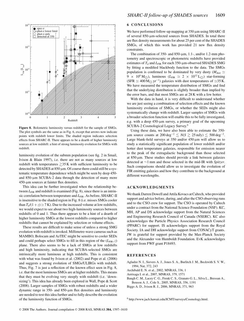
Figure 8. Bolometric luminosity versus redshift for the sample of SMGs.The plot symbols are the same as in Fig. 6, except that arrows now indicatepoints with redshift lower limits. The shaded region indicates selectioneffects from SHARC-II. There appears to be a dearth of higher luminositysources at low redshift: a hint of strong luminosity evolution for SMGs withredshift.

luminosity evolution of the submm population (see fig. 2 in Smail,Ivison & Blain 1997), i.e. there are not as many sources at lowredshift with temperatures �35 K with sufficient luminosity to bedetected by SHADES at 850 μm. Of course there could still be a sys-tematic temperature dependence which might be seen by deep 450-and 850-μm SCUBA-2 data through the detection of many more450-μm sources at fainter flux densities.

This idea can be further investigated when the relationship be-tween LFIR and redshift is examined (Fig. 8), since there is an intrin-sic correlation between temperature and LFIR. As before, SHARC-IIis insensitive to the shaded region in Fig. 8 (i.e. misses SMGs coolerthan Td/(1 + z) � 7 K). Due to the increased volume at low redshifts,we would expect to see about two high-luminosity sources betweenredshifts of 0 and 1. Thus there appears to be a hint of a dearth ofhigher luminosity SMGs at the lowest redshifts compared to higherredshifts that cannot be explained by selection or volume effects.

These results are difficult to make sense of unless a strong SMGevolution with redshift is invoked. Millimetre-wave cameras such asMAMBO, Bolocam and AzTEC might be sensitive to cooler SEDsand could perhaps select SMGs to fill in this region of the (LFIR, z)plane. There also seems to be a lack of SMGs at low redshiftsand high luminosity, indicating that SCUBA-selected SMGs areintrinsically more luminous at high redshifts. This is consistentwith what was found by Ivison et al. (2002) and Pope et al. (2006)and suggests a strong evolution of SMGs/ULIRGs with redshift.Thus, Fig. 7 is just a reflection of the known effect seen in Fig. 8,i.e. that the most luminous SMGs are at higher redshifts. This meansthat they must be evolving very steeply with redshift (i.e. ‘down-sizing’). This idea has already been explored in Wall, Pope & Scott(2008). Larger samples of SMGs with robust redshifts and a widerdynamic range in 350- and 850-μm flux densities and luminosityare needed to test this idea further and to fully describe the evolutionof the luminosity function of SMGs.

6 C O N C L U S I O N S

We have performed follow-up mapping at 350 μm using SHARC-IIof several 850-μm-selected sources from SHADES. In total thereare flux density measurements for about 25 per cent of the SHADESSMGs, of which this work has provided 21 new flux densityconstraints.

The combination of 350- and 850-μm, 1.1-, and/or 1.2-mm pho-tometry and spectroscopic or photometric redshifts have providedestimates of Td and LFIR for each 350-μm-observed SHADES SMGby fitting a modified blackbody function to the data. The SMGspopulation is confirmed to be dominated by very dusty (Mdust �9 × 108 M�), luminous (LFIR � 2 × 1012 L�) star-forming(SFR � 400 M� yr−1) galaxies with dust temperatures of �35 K.We have measured the temperature distribution of SMGs and findthat the underlying distribution is slightly broader than implied bythe error bars, and that most SMGs are at 28 K with a few hotter.

With the data in hand, it is very difficult to understand whetherwe are just seeing a combination of selection effects and the knownluminosity evolution of SMGs, or whether the SEDs might alsosystematically change with redshift. Larger samples of SMGs witha broader selection function will enable this to be fully investigated,e.g. with a deep 450-μm survey, a primary goal of the upcomingSCUBA-2 Cosmological Legacy Survey.6

Using these data, we have also been able to estimate the 350-μm source counts at 200 deg−2 � N(S � 25 mJy) � 500 deg−2.Large blank-field surveys at 350 and/or 450 μm will allow us tostudy a statistically significant population of lower redshift and/orhotter dust temperature galaxies, responsible for emission nearerto the peak of the extragalactic background than those selectedat 850 μm. These studies should provide a link between galaxiesdetected at ∼1 mm and those selected in the mid-IR with Spitzer.Such comparisons should allow us to investigate the evolution ofFIR emitting galaxies and how they contribute to the background atdifferent wavelengths.

AC K N OW L E D G M E N T S

We thank Darren Dowell and Attila Kovacs at Caltech, who providedsupport and advice before, during, and after the CSO observing runsand to the CSO crew for support. The CSO is operated by Caltechunder a contract from the National Science Foundation (NSF). KC,MH, AP and DS acknowledge support from the Natural Sciencesand Engineering Research Council of Canada (NSERC). KC alsoacknowledges the Particle Physics Association Research Council(PPARC) for support. IS acknowledges support from the RoyalSociety. IA and DH acknowledge support from CONACyT grants.JW is grateful for support provided by the Max-Planck Societyand the Alexander von Humboldt Foundation. EvK acknowledgessupport from FWF grant P18493.

REFERENCES

Agladze N. I., Sievers A. J., Jones S. A., Burlitch J. M., Beckwith S. V. W.,1994, Nat, 372, 243

Archibald E. N. et al., 2002, MNRAS, 336, 1Aretxaga I. et al., 2007, MNRAS, 379, 1571Baugh C. M., Lacey C. G., Frenk C. S., Granato G. L., Silva L., Bressan A.,

Benson A. J., Cole S., 2005, MNRAS, 356, 1191Biggs A. D., Ivison R. J., 2006, MNRAS, 371, 963

6 http://www.jach.hawaii.edu/JCMT/surveys/Cosmology.html.



Blain A. W., Smail I., Ivison R. J., Kneib J.-P., Frayer D. T., 2002, Phys.Rep., 369, 111

Blain A. W., Barnard V. E., Chapman S. C., 2003, MNRAS, 338, 733Chapman S. C., Lewis G. F., Scott D., Borys C., Richards E., 2002, ApJ,

570, 557Chapman S. C., Blain A. W., Ivison R. J., Smail I. R., 2003, Nat, 422, 695Chapman S. C., Blain A. W., Smail I., Ivison R. J., 2005, ApJ, 622, 772Clements D. et al. 2008, MNRAS, in pressCoppin K., Halpern M., Scott D., Borys C., Chapman S. C., 2005, MNRAS,

357, 1022Coppin K. et al., 2006, MNRAS, 372, 1621Devlin M. et al., 2004, in Zmvidzinas J., Holland W. S., Withington S., eds,

SPIE Conf. Proc. Vol. 5498, Millimeter and Submillimeter Detectors forAstronomy II, SPIE, Bellingham WA, p. 42

Dowell C. D. et al., 2003, in Phillips T. G., Zmuidzinas J., eds, SPIE Conf.Proc. Vol. 4855, Millimeter and Submillimeter Detectors for Astronomy.SPIE, Bellingham WA, p. 73

Dunlop J. S., 2001, New Astron. Rev., 45, 609Dunne L., Eales S., 2001, MNRAS, 327, 697Dunne L., Eales S., Edmunds M., Ivison R., Alexander P., Clements D. L.,

2000, MNRAS, 315, 115Dunne L., Eales S., Edmunds M., 2003, MNRAS, 341, 589Edmunds M. G., Eales S. A., 1998, MNRAS, 299, L29Farrah D., Afonso J., Efstathiou A., Rowan-Robinson M., Fox M., Clements

D., 2003, MNRAS, 343, 585Greve T. R., Ivison R. J., Bertoldi F., Stevens J. A., Dunlop J. S., Lutz D.,

Carilli C. L., 2004, MNRAS, 354, 779Guiderdoni B., Hivon E., Bouchet F. R., Maffei B., 1998, MNRAS, 295,

877Hildebrand R. H., 1983, QJRAS, 24, 267Holland W. S. et al., 1999, MNRAS, 303, 659Holland W. S. et al., 2006, in Zmuidzinas J., Holland W. S., Withington

S., Duncan W. D., eds, SPIE Conf. Proc. Vol. 6275, Millimeter andSubmillimeter Detectors and Instrumentation III. SPIE, Bellingham WA,p. 45

Hughes D. H., Dunlop J. S., Rawlings S., 1997, MNRAS, 289, 766Huynh M. T., Pope A., Frayer D. T., Scott D., 2007, ApJ, 659, 305Ivison R. J., 2006, Conf. Proc. Sintra, preprint (astro-ph/0701453)Ivison R. J. et al., 2002, MNRAS, 337, 1Ivison R. J. et al., 2005, MNRAS, 364, 1025Ivison R. J. et al., 2007, MNRAS, 380, 199Kennicutt R. C., 1998, ARA&A, 36, 189Khan S. et al., 2005, ApJ, 631, 9Khan S. et al., 2007, ApJ, 665, 973Kovacs A., 2006, PhD thesis, CaltechKovacs A., Chapman S. C., Dowell C. D., Blain A. W., Ivison R. J., Smail

I., Phillips T. G., 2006, ApJ, 650, 592Lagache G. et al., 2004, ApJS, 154, 112Laurent G. T. et al., 2005, ApJ, 623, 742Laurent G. T., Glenn J., Egami E., Rieke G. H., Ivison R. J., Yun M. S.,

Aguirre J. E., Maloney P. R., 2006, ApJ, 643, 38Leong M. M., 2005, URSI Conf. Sec., J3-J10, 426Lilly S. J., Eales S. A., Gear W. K. P., Hammer F., Le Fevre O., Crampton

D., Bond R. J., Dunne L., 1999, ApJ, 518, 641Mortier A. M. J. et al., 2005, MNRAS, 363, 563Pilbratt G. L., 2003, in Mather J. C., ed., SPIE Conf. Proc. Vol.

4850, IR Space Telescopes and Instruments. SPIE, Bellingham WA,p. 586

Pope A., Borys C., Scott D., Conselice C., Dickinson M., Mobasher B.,2005, MNRAS, 358, 149

Pope A. et al., 2006, MNRAS, 370, 1185Sajina A., Lacy M., Scott D., 2005, ApJ, 621, 256Salpeter E. E., 1955, ApJ, 121, 161Sanders D. B., Mirabel F., 1996, ARA&A, 34, 749Smail I., Ivison R. J., Blain A. W., 1997, ApJ, 490, L5Spergel D. N. et al., 2003, ApJS, 148, 175Tauber J. A., 2004, Adv. Space Res., 34, 491Wall J. V., Pope A., Scott D. S., 2008, MNRAS, 383, 435

APPENDI X A : EFFECTI VE EXPOSURE T IMES

When describing astronomical data, it is common and straightfor-ward to give total observation times, or perhaps in chopped systemsthe total time on source. These times give an indication of theamount of effort expended to collect the data. However, becausethe atmosphere is far from transparent at submm wavelengths (evenin the atmospheric windows) and the transmission is so weatherdependent, the total exposure time does not give a good indicationof data quality or expected noise level in the final output. It is moreuseful to refer to the effective total exposure which is the noise-squared weighted sum of exposure times referred to a completelytransparent atmosphere.

The optical depth of the atmosphere in a given direction is de-termined from the wavelength dependent optical depth at zenith,τ λ, and the cosecant of the zenith angle, θ , of observation, calledthe airmass, A. Thus, the strength of an observed astronomical fluxdensity, So is

So = S e−τλ(t)A(θ). (A1)

At 850 μm, the zenith optical depth, τ 850, ranges from, say, 0.16in very good weather to 0.7 in bad weather, and the optical depthat 350 or 450 μm is typically seven times higher. The first step incombining data collected at different times of night with differentvalues of τ λ and A is to correct So for atmospheric absorption bymultiplying by eτλ A (see Archibald et al. 2002).

After correcting for atmospheric transients, etc., but not opacity,the output noise at the detector is fairly independent of atmosphericopacity, at least for SCUBA operating on the James Clerk MaxwellTelescope on Mauna Kea at 450 and 850 μm, and for SHARC-IIoperating at 350 μm at the CSO also on Mauna Kea. Therefore, theeffective noise of an observation is inflated exponentially in τ λ andA. The sum

teff =∑

�toe2 τλ(t)A (A2)

is the integration time that would be required with a completelytransparent atmosphere to get the same noise level as a given noise-squared weighted sum of observations, each of size �to. We callthis the effective exposure time and find that tracking this quantityduring observations is an effective way to monitor experimentalprogress.

In practice, the optical depth as a function of time is obtainedfrom automated measurements made at the CSO at 225 GHz every10 min. The optical depths at submm wavelengths are very wellcorrelated with these values and one multiplies τ 225 GHz by about4 and 24 to get optical depths for SCUBA at 850 and 450 μm,respectively, and by 26 to get τ for SHARC-II at 350 μm (Archibaldet al. 2002).

As a numerical example, observation of a source which risesthrough transit with an average airmass of 1.3 and τ 225 GHz = 0.05for 4-h results in effective exposure times of 2.4 h at 850 μm,20.7 min at 450 μm with SCUBA, and 9.5 min with SHARC-II. Theshorter effective times at shorter wavelengths are a consequenceof the fact that the atmosphere is not very transparent at thosewavelengths. This is why space experiments like Herschel-SPIREand BLAST are useful even with comparatively small apertures,and why neither of those experiments carries an 850-μm channel.Experience has shown that effective exposures of between 500 and600 s with SHARC-II are often sufficient to detect faint extragalactichigh-redshift sources.

This paper has been typeset from a TEX/LATEX file prepared by the author.


The SCUBA HAlf Degree Extragalactic Survey – VI....

Documents

Transcript of The SCUBA HAlf Degree Extragalactic Survey – VI....