Dan Schultz August 20, 2015
86
Notes on Modular Forms Dan Schultz August 20, 2015
Transcript of Dan Schultz August 20, 2015
Notes on Modular Forms
Dan Schultz
August 20, 2015
Contents
0.1 Notation . . . . . . . . . . . . . . . . . . . . . . . . . . . . . . . . . . . . . . . . . . . 2
1 Introduction 41.1 Partitions and the η function . . . . . . . . . . . . . . . . . . . . . . . . . . . . . . . 41.2 Sums of squares and the θ function . . . . . . . . . . . . . . . . . . . . . . . . . . . . 41.3 Ramanujan’s τ Function . . . . . . . . . . . . . . . . . . . . . . . . . . . . . . . . . . 51.4 Mock Modular Forms . . . . . . . . . . . . . . . . . . . . . . . . . . . . . . . . . . . . 51.5 Special Values of the j Function . . . . . . . . . . . . . . . . . . . . . . . . . . . . . . 6
2 Elliptic Functions and Basic Modular Forms on SL2(Z) 72.1 Theory of Elliptic Functions . . . . . . . . . . . . . . . . . . . . . . . . . . . . . . . . 72.2 The Weierstrass ℘ Function . . . . . . . . . . . . . . . . . . . . . . . . . . . . . . . . 82.3 Eisenstein Series . . . . . . . . . . . . . . . . . . . . . . . . . . . . . . . . . . . . . . 92.4 Modular Discriminant ∆(τ) and Klein’s Absolute Invariant j(τ) . . . . . . . . . . . . 102.5 Basic Properties of SL2(Z) . . . . . . . . . . . . . . . . . . . . . . . . . . . . . . . . . 112.6 The η function and E2 . . . . . . . . . . . . . . . . . . . . . . . . . . . . . . . . . . . 122.7 Recursions for the Eisenstein Series . . . . . . . . . . . . . . . . . . . . . . . . . . . . 152.8 Elliptic Θ Functions . . . . . . . . . . . . . . . . . . . . . . . . . . . . . . . . . . . . 152.9 Γ(2) and the Asymptotic of Θ Near the Cusps . . . . . . . . . . . . . . . . . . . . . . 192.10 Addition Formulas . . . . . . . . . . . . . . . . . . . . . . . . . . . . . . . . . . . . . 232.11 Γ(3) and the Asymptotic of η Near the Cusps . . . . . . . . . . . . . . . . . . . . . . 242.12 Exercises . . . . . . . . . . . . . . . . . . . . . . . . . . . . . . . . . . . . . . . . . . . 28
3 Theory of Modular Forms on SL2(Z) 313.1 Definition of a Modular Form . . . . . . . . . . . . . . . . . . . . . . . . . . . . . . . 313.2 Valence Formula . . . . . . . . . . . . . . . . . . . . . . . . . . . . . . . . . . . . . . 323.3 Dimension Formulas and Generators . . . . . . . . . . . . . . . . . . . . . . . . . . . 333.4 Applications to Identities . . . . . . . . . . . . . . . . . . . . . . . . . . . . . . . . . . 343.5 Exercises . . . . . . . . . . . . . . . . . . . . . . . . . . . . . . . . . . . . . . . . . . . 35
4 Theory of Modular Forms on Congruence Subgroups of SL2(Z) 364.1 Definition of modular forms on Γ with [Γ(1) : Γ] <∞ . . . . . . . . . . . . . . . . . . 364.2 Dimension formulas . . . . . . . . . . . . . . . . . . . . . . . . . . . . . . . . . . . . . 384.3 Counting εi for Γ(N) and Γ1(N) and Γ0(N) . . . . . . . . . . . . . . . . . . . . . . . 404.4 General properties of Ak(Γ) . . . . . . . . . . . . . . . . . . . . . . . . . . . . . . . . 424.5 Working with finite index subgroups of Γ(1) . . . . . . . . . . . . . . . . . . . . . . . 464.6 Γ(2) . . . . . . . . . . . . . . . . . . . . . . . . . . . . . . . . . . . . . . . . . . . . . 524.7 Building congruence modular forms N from Klein Forms . . . . . . . . . . . . . . . . 534.8 Building congruence modular forms from η products . . . . . . . . . . . . . . . . . . . 554.9 Γ(N) and regular polyhedron . . . . . . . . . . . . . . . . . . . . . . . . . . . . . . . 57
1
4.10 Representations by x2 + y2 . . . . . . . . . . . . . . . . . . . . . . . . . . . . . . . . . 644.11 Building congruence modular forms from Θ functions . . . . . . . . . . . . . . . . . . 654.12 Representations by x2 + xy + y2 other quadratic forms . . . . . . . . . . . . . . . . . 674.13 Subgroups up to index 7: non-congruence examples . . . . . . . . . . . . . . . . . . . 69
5 Hecke Operators 745.1 Definition of the Hecke operators . . . . . . . . . . . . . . . . . . . . . . . . . . . . . 745.2 Eigenforms . . . . . . . . . . . . . . . . . . . . . . . . . . . . . . . . . . . . . . . . . 745.3 Newforms . . . . . . . . . . . . . . . . . . . . . . . . . . . . . . . . . . . . . . . . . . 74
6 Modular Forms mod p 756.1 The structure of modular forms on SL2(Z) mod p . . . . . . . . . . . . . . . . . . . . 756.2 The congruences for p(n) mod 5,7,11 are the Unique Ramanujan Congruences . . . . 75
6.3 24n ≡ 1 mod 5a7b11c implies p(n) ≡ 0 mod 5a7bb2c+111c . . . . . . . . . . . . . . . . 75
7 Modular Equations and Singular Values 767.1 Modular equations for j . . . . . . . . . . . . . . . . . . . . . . . . . . . . . . . . . . 767.2 Modular equations for the Weber functions . . . . . . . . . . . . . . . . . . . . . . . . 777.3 Quadratic Forms . . . . . . . . . . . . . . . . . . . . . . . . . . . . . . . . . . . . . . 777.4 Singular Values of the j Function . . . . . . . . . . . . . . . . . . . . . . . . . . . . . 787.5 Singular Values of the Weber Functions . . . . . . . . . . . . . . . . . . . . . . . . . . 797.6 The Class Number One Problem . . . . . . . . . . . . . . . . . . . . . . . . . . . . . . 807.7 Singular Values of the η Function . . . . . . . . . . . . . . . . . . . . . . . . . . . . . 80
8 Hypergeometric Functions 818.1 Basic Properties of the 2F1(x) and 3F2(x) Series . . . . . . . . . . . . . . . . . . . . . 818.2 Jacobi’s Inversion Formula and Generalizations . . . . . . . . . . . . . . . . . . . . . 818.3 Solution of the General Quintic by Modular Functions . . . . . . . . . . . . . . . . . 81
9 Mock Modular Forms 84
0.1 Notation
Symbol Meaningq e2πiτ
qa e2πiaτ (not (e2πiτ )a)qaz e2πiaz
e(z) exp(2πiz)ζab root of unity e(a/b)
log z the logarithm with −π < Im log z ≤ πab exp b log a
(x; q)n∏n−1
k=0(1− xqk)(x; q)∞
∏∞k=0(1− xqk), for |q| < 1
℘(z|ω1, ω2) Weierstrass ℘ function for the lattice ω1Z + ω2Z
2
ζ(z|ω1, ω2) Weierstrass ζ functionσ(z|ω1, ω2) Weierstrass σ function
℘(z|τ) ℘(z|τ, 1)η(τ) Dedekind’s η function q1/24(q; q)∞j(τ) E4(τ)3η(τ)−24
γ2(τ) j1/3 = E4(τ)η(τ)−8
γ3(τ) (j − 1728)1/2 = E6(τ)η(τ)−12
Θ[~v](z|τ) general elliptic Θ function with characteristic ~vΘi(z|τ) Jacobi’s four Θ functions with half-integer characteristics
Θi(z) Θi(z|τ)Θi(τ) Θi(0|τ)Γ(N) M ∈ SL2(Z) |M ≡ ( 1 0
0 1 ) mod NΓ1(N) M ∈ SL2(Z) |M ≡ ( 1 ∗
0 1 ) mod NΓ1(N) M ∈ SL2(Z) |M ≡ ( 1 0
∗ 1 ) mod NΓ0(N) M ∈ SL2(Z) |M ≡ ( ∗ 0
∗ ∗ ) mod NΓ0(N) M ∈ SL2(Z) |M ≡ ( ∗ ∗0 ∗ ) mod NΓ0
0(N) M ∈ SL2(Z) |M ≡ ( ∗ 00 ∗ ) mod N
u.v dot product of two vectorsu.M product of vector u interpreted as a row vector and the matrix MM.v product of matrix M and the vector v interpreted as a column vector
3
Chapter 1
Introduction
The generating functions for many interesting combinatorial objects turn out to be modular forms.
1.1 Partitions and the η function
We have
1
(q; q)∞= (1 + q + q2 + q3 + · · · )(1 + q2 + q4 + q6 + · · · )(1 + q3 + q6 + q9 + · · · ) · · ·
=∞∑n=0
p(n)qn,
where p(n) is the number of partitions of n. We have the properties
• p(5n+ 4) ≡ 0 mod 5
• p(7n+ 5) ≡ 0 mod 7
• p(11n+ 6) ≡ 0 mod 11
• p(59413n+ 111247) ≡ 0 mod 13 (see [2])
The three primes 5, 7, 11 are unique in this way. Similar congruences hold at powers of these primes.
1.2 Sums of squares and the θ function
Setθ(τ) =
∑n∈Z
qn2
.
Then, the generating function for #(x1, . . . , xk)|n = x21 + · · · + x2
k, which is the number of repre-sentations of n by the sum of k squares, is θ(τ)k. If χ4 is the non-trivial character modulo 4 and 4|cand ad− bc = 1, will we see that θ satisfies the weight 1/2 relation
θ
(aτ + b
cτ + d
)=( cd
)χ4(d)−1/2
√cτ + dθ(τ),
and characterize all functions that satisfy even powers of this functional equation. This leads to andeasy proof of
(x, y) ∈ Z2|n = x2 + y2 = 4∑d|n
χ4(d).
4
Similar formulas exists for other θ functions.
(x, y) ∈ Z2|n = x2 + xy + y2 = 6∑d|n
χ3(d).
1.3 Ramanujan’s τ Function
Define τ(n) by
η(τ)24 = q(q; q)24∞ =:
∞∑n=1
τ(n)qn.
The following properties were observed by Ramanujan.
• τ(mn) = τ(m)τ(n) for (m,n) = 1
• τ(pk+1) = τ(pk)τ(p)− p11τ(pk−1)
• τ(p) ≤ 2p11/2
• τ(n) ≡ σ11(n) mod 691
The weight 12 relation is satisfied by η(τ)24 is
η
(aτ + b
cτ + d
)24
= (cτ + d)12η(τ)24.
The first two are equivalent to the Euler product
f(s) =∞∑n=1
τ(n)
ns=∏p
1
1− τ(p)p−s + p11−2s,
and the weight 12 transformation formula gives the reflection formula
f(s)Γ(s)
(2π)s=f(12− s)Γ(12− s)
(2π)12−s .
1.4 Mock Modular Forms
By considering the Durfee square, we have
1
(q; q)∞=∞∑n=0
qn2
(q; q)2n
,
which is essentially a (weak) modular form of weight −1/2. The function
f(τ) =∞∑n=0
qn2
(−q; q)2n
turns out to not be modular, but can be made modular by adding some non-holomorphic function toit. Set
F (z) = q−1z f(24z) +
√−8
∫ i∞
−z
∑n∈Z χ12(n)nqn
2√−i(τ + z)
dτ .
If ad− bc = 1 and 144|c, we have
F
(aτ + b
cτ + d
)=
(12c
d
)χ4(d)−1/2
√cτ + dF (τ).
5
1.5 Special Values of the j Function
Let K = Q(√−d) be an imaginary quadratic field and let Z + Zτ be its ring of integers. Then,
j(τ) is an algebraic integer of degree h(−d) over Q, and K(j(τ)) is the maximal unramified Abelianextension of K.
6
Chapter 2
Elliptic Functions and Basic ModularForms on SL2(Z)
2.1 Theory of Elliptic Functions
Definition 2.1.1. Let ω1, ω2 ∈ C with Im(ω1/ω2) > 0. An elliptic function modulo Zω1 + Zω2 is ameromorphic function C→ C satisfying
f(z) = f(z + ω1) = f(z + ω2).
For the order of a non-constant function at a point z0, we say ordz0(f(z)) = n if
f(z) = (z − z0)n(c+O(z − z0)), c 6= 0,
and ord f(z), the (total) order of the function f(z), is the number of poles of f counted according tomultipliticy (modulo Λ).
Proposition 2.1.2. Let f be a non-constant elliptic function modulo Λ. Then,
1.∑
z∈C/Λ resz(f) = 0
2.∑
z∈C/Λ ordz(f) = 0
3.∑
z∈C/Λ z ordz(f) ∈ Λ
4. ord f ≥ 2.
Proof. Let C denote the counterclockwise traversal of the parallelogram with vertices 0, ω2, ω2+ω1, ω1.Then, ∑
z∈C/Λ
resz(f) =1
2πi
∫C
f(z)dz = 0
∑z∈C/Λ
ordz(f) =1
2πi
∫C
f ′(z)
f(z)dz = 0
7
since integrals along opposite sides cancel. Next∑z∈C/Λ
z ordz(f) =1
2πi
∫C
zf ′(z)
f(z)dz
=1
2πi
∫ ω1
0
zf ′(z)
f(z)− (ω2 + z)f ′(ω2 + z)
f(ω2 + z)dz
+1
2πi
∫ ω2
0
−zf′(z)
f(z)+
(ω1 + z)f ′(ω1 + z)
f(ω1 + z)dz
= −ω2 ·1
2πi
∫ ω1
0
f ′(z)
f(z)dz
+ ω1 ·1
2πi
∫ ω2
0
f ′(z)
f(z)dz
= −ω2
(1
2πilog f(z)
]ω1
0
)+ ω1
(1
2πilog f(z)
]ω2
0
)∈ Λ
since ω1 (and ω2) is a period of the function f(z), so the logarithm must change by an integral multipleof 2πi. For (4), if f had order 0, then it has no poles, and is thus bounded so is constant by Liouville’stheorem. If f had order 1, then it has a simple pole with non-zero residue, which contradicts (1).
Later will we see that part (3) of Proposition 2.1.2 has a converse, that is, we can construct anelliptic function with any poles and zeros that satisfy (3).
2.2 The Weierstrass ℘ Function
For a lattice Λ, let Λ′ denote Λ− 0. Set
℘(z|ω1, ω2) =1
z2+∑ω∈Λ′
1
(z + ω)2− 1
ω2,
℘′(z|ω1, ω2) =∑ω∈Λ
−2
(z + ω)3,
Gk(ω1, ω2) =∑ω∈Λ′
1
ωk.
The sum for ℘(z) is arranged so that
1
(z + ω)2− 1
ω2= O(w−3)
which makes the sum over Λ absolutely convergent. The series for G2 is not absolutely convergent,so this is not a proper definition of G2. Later, when defining E2, we will fix the order of summation.
Proposition 2.2.1. Set Λ = Zω1 + Zω2. Then, ℘(z|ω1, ω2) is an elliptic function of order 2 mod Λ,and we have:
1. The power series expansion
℘(z|ω1, ω2) =1
z2+∞∑k=1
(2k + 1)G2k+2(ω1, ω2)z2k.
8
2. For λ 6= 0 and integers a, b, c, d with ad− bc = 1,
℘(z|ω1, ω2) = λ2℘(λz|λω1, λω2),
℘(z|ω1, ω2) = ℘(z|aω1 + bω2, cω1 + dω2).
3. The differential equation (set g2 = 60G4(ω1, ω2), g3 = 140G6(ω1, ω2))
℘′(z)2 = 4℘(z)3 − g2℘(z)− g3.
Proof. From the definitions, it is clear that ℘′(z) is elliptic modulo Λ and ℘(z) is an even function.Let ω ∈ Λ. Since ℘′(z + ω) = ℘′(z), it follows that ℘(z + ω) = ℘(z) + η for some constant η. Settingz = −ω/2 shows that η = 0. For (2), set M = ( a bc d ). Then,
℘(z|aω1 + bω2, cω1 + dω2) =1
z2+
∑~n∈Z2−0,0
1
(z + ~n.M.(ω1, ω2)ᵀ)2− 1
(~n.M.(ω1, ω2)ᵀ)2
=1
z2+
∑~m∈Z2−0,0
1
(z + ~m.(ω1, ω2)ᵀ)2− 1
(~m.(ω1, ω2)ᵀ)2
= ℘(z|ω1, ω2).
Since det(M) = 1, ~n.M ranges over all of Z2 − 0, 0 and includes each point once, the change ofvariables ~m = ~n.M is justified.
For (3),
℘′(z)2 =4
z6− 24G4
z2− 80G6 +O(z2)
4℘(z)3 =4
z6+
36G4
z2+ 60G6 +O(z2)
60℘(z) =60G4
z2+O(z2).
From this it is clear that ℘′(z)2−4℘(z)3+60G4℘(z) is an entire elliptic function, hence it is a constant.This constant is also easily seen to be −140G6.
2.3 Eisenstein Series
Due to the homogeneity property in Proposition 2.2.1, without loss of generality we can set ω1 = τand ω2 = 1. In this case we have
℘(z|τ, 1) = (cτ + d)−2℘
(z
cτ + d
∣∣∣aτ + b
cτ + d, 1
),
which shows that the power series coefficients satisfy
G2k
(aτ + b
cτ + d, 1
)= (cτ + d)2kG2k(τ, 1), k ≥ 2.
It will be convenient to have a normalization of these functions E2k(τ) with E2k(i∞) = 1. For k ≥ 1,set
E2k(τ) =G2k(τ, 1)
G2k(i∞, 1)
=1
2ζ(2k)
∞∑m=−∞
∞∑n=−∞
(m,n)6=(0,0)
1
(mτ + n)2k.
9
Proposition 2.3.1. The Eisenstein series E2k have the following properties.
1. For k ≥ 1, we have
E2k(τ) = 1 +2
ζ(1− 2k)
∞∑n=1
n2k−1qk
1− qk.
2. For k ≥ 2, E2k(τ) is a holomorphic function H→ C satisfying
E2k
(aτ + b
cτ + d
)= (cτ + d)2kE2k(τ).
We cannot conclude the last property for k = 1 because the series defining G2(τ, 1) is not absolutelyconvergent. It turns out that E2(τ) has a similar functional equation with a small “error” term.
Proof. Using Exercise 2.12.3,
E2k(τ) =1
2ζ(2k)
(∞∑n=1
2
(n)2k+∞∑m=1
∞∑n=−∞
1
(mτ + n)2k+
1
(−mτ + n)2k
)
= 1 +1
ζ(2k)
∞∑m=1
∞∑n=−∞
1
(mτ + n)2k
= 1 +2
ζ(1− 2k)
∞∑m=1
∞∑j=1
j2k−1qjm
= 1 +2
ζ(1− 2k)
∞∑j=1
j2k−1 qj
1− qj
2.4 Modular Discriminant ∆(τ ) and Klein’s Absolute Invari-
ant j(τ )
Let ei(τ) be the roots of the cubic polynomial in the differential equation for ℘, that is,
(℘′)2 = 4℘3 − g2℘− g3
= 4(℘− e1)(℘− e2)(℘− e3).
The discriminant of the cubic polynomial is therefore
∆(τ) : = 16(e1 − e2)2(e2 − e3)2(e3 − e1)2
= −64 (e1e2 + e1e2 + e3e1) 3 − 432e21e
22e
23
= g32 − 27g2
3,
where we have used
0 = e1 + e2 + e3,
g2 = −4 (e1e2 + e2e3 + e3e1) ,
g3 = 4e1e2e3.
10
Also, set
j(τ) =1728g2(τ)3
∆(τ).
This function is known as Klein’s absolute invariant, or just the j function.
Proposition 2.4.1. For ∆(τ) and j(τ) we have
1. Representation in E4 and E6 and q-series expansions:
∆(τ) =64π12
27(E3
4 − E26) = (2π)12q +O(q2),
j(τ) =1728E3
4
E34 − E2
6
=1
q+ 744 +O(q).
2. For ad− bc = 1,
∆
(aτ + b
cτ + d
)= (cτ + d)12∆(τ),
j
(aτ + b
cτ + d
)= j(τ).
3. At τ = i∞, ∆(τ) vanishes and j(τ) blows up.
4. ∆(τ) does not vanish (equiviently, j(τ) has no poles) at any τ ∈ H.
Proof. Exercise 2.12.2.
2.5 Basic Properties of SL2(Z)
For the Eisenstein series, we were able to find the transformation formula for any a, b, c, d directly.However, in most cases we will just prove the transformation formula for specific a, b, c, d and hopethat the result for general a, b, c, d can be obtained by iterating these special cases. Set
Γ(1) = SL2(Z),
i.e. the “modular group” or “full modular group”. A matrix in SL2(Z) acts on H via(a bc d
): τ 7→ aτ + b
cτ + d
Note that
Im
(aτ + b
cτ + d
)=
Im τ
|cτ + d|2(2.5.1)
Two important elements are S and T :
S =
(0 −11 0
): τ 7→ −1
τ,
T =
(1 10 1
): τ 7→ τ + 1.
Also setF =
τ ∈ H | −1
2≤ Re τ ≤ 1
2and |τ | ≥ 1
.
The left and right edges with Re τ = ±12
are identified via T , and the left and right edges of F on|τ | = 1 are identified via S. We will also formally include i∞ in F as well.
11
Proposition 2.5.1. For Γ(1), we have
1. F is a fundamental domain for H/Γ(1) with the appropriate edges identitfied.
2. S and T generate Γ(1)/± I.
3. For any τ ∈ F the isotropy subgroup Γ(1)τ := g ∈ Γ(1)|gτ = τ is ±I except in the cases
• τ = i∞, Γ(1)τ := ±T kk∈Z• τ = i, Γ(1)τ := ±I, S• τ = e(1/3), Γ(1)τ := ±I, ST, (ST )2• τ = e(1/6), Γ(1)τ := ±I, TS, (TS)2
Proof. Sketch of (1) and (3): Given τ ∈ H, we can apply T and S to get a point in F by repeatingthe following steps. Apply T k to get τ inside −1
2≤ Re τ ≤ 1
2. If |τ | < 1 apply S. This must terminate
with a point in F because Im τ only increases throughout the process. Now suppose τ1, τ2 ∈ F withIm τ2 ≥ Im τ1 are related by τ2 = (aτ1 + b)/(cτ1 + d). From (2.5.1), this means that |cτ1 + d| ≤ 1.Since τ1 is in F this restricts c to c = 0, 1,−1.
(2). Given g ∈ Γ(1) take any τ in the interior of F . Use S and T to get gτ back into F and use(1) to conclude that g is a product of T and S (modulo ±I).
2.6 The η function and E2
The logarithmic derivative ofη(τ) := q1/24(q; q)∞
is simply related to E2(τ).
1
2πi
d
dτlog η(τ) =
1
2πi
d
dτ
(2πiτ
24+∞∑n=1
log(1− qn)
)
=1
24+ q
d
dq
∞∑n=1
log(1− qn)
=1
24−∞∑n=1
nqn
1− qn
=1
24E2(τ).
Lemma 2.6.1 (Poisson Summation Formula for Cosine). Under suitable restrictions of the functionf , if
fc(y) =
∫ ∞−∞
f(x) cos(2πxy)dx,
then∞∑
n=−∞
fc(n) =f(0)
2+∞∑n=1
f(n).
Proposition 2.6.2. For ( a bc d ) ∈ Γ(1), we have
12
1. E2 transformation:
E2 (τ + 1) = E2(τ),
τ−2E2
(−1
τ
)= E2(τ) +
12
2πiτ,
(cτ + d)−2E2
(aτ + b
cτ + d
)= E2(τ) +
12c
2πi(cτ + d).
2. η transformation:
η (τ + 1) = e
(1
24
)η(τ),
η
(−1
τ
)=√−iτη(τ),
η
(aτ + b
cτ + d
)= εη
(a bc d
)√−i(cτ + d)η(τ),
where εη( a bc d ) is some 24th root of unity.
Proof. The first parts of (1) and (2) are trivial, so we start with the second part of (1). In Lemma2.6.1 set
f(x) = −24∞∑n=1
xe(nτx) =−24xqx
1− qx,
f(0) =24
2πiτ.
The result
fc(y) =1
2ζ(2)
∞∑n=1
1
(nτ + y)2+
1
(−nτ + y)2
=1
2ζ(2)
∑n∈Zn6=0
1
(nτ + y)2
is elementary, so the assertion of Lemma 2.6.1 gives
1
2ζ(2)
∞∑m=−∞
∞∑n=−∞n6=0
1
(nτ +m)2=
12
2πiτ− 24
∞∑n=1
nqn
1− qn,
or,1
2ζ(2)
(−2ζ(2) + τ−2G2
(−1
τ
))=
12
2πiτ− 1 + E2(τ),
which is the second part of (1). The second part of (2) follows from integrating the second part of (1)and using τ = i to evaluate the constant of integration. The third parts of each follow from the firsttwo since S and T generate Γ(1).
13
Note that the η function is non-vanishing on H so we may define a logarithm
log η(τ) :=2πiτ
24+∞∑n=1
log (1− qn) .
This also entails that we may define a logarithm of the corresponding multiplier system
log εη( a bc d ) := log η
(aτ + b
cτ + d
)− 1
2log(
√−i(cτ + d))− log η(τ).
Now we give a formula for log εη( a bc d ) in terms of Dedekind sums and a slightly simpler formula for
its exponential εη( a bc d ). For odd primes p let(cp
)be the usual Legendre symbol. Extend this to all
positive odd d by means of the prime factorization d = pe11 · · · penn via( cd
)=
(c
p1
)e1· · ·(c
pn
)en.
Then, extend to negative odd d by( cd
)= (−1)
sign(d)−12
sign(c)−12
(c
|d|
).
Note we have the generalized quadratic reciprocity and periodicity( cd
)= (−1)
d−12
c−12
(d
|c|
), for c, d odd(
c+ d
d
)=
−(cd
), d < 0 and sign(c) 6= sign(c+ d)
+(cd
), otherwise
,
(d
c+ 2d
)=
−(dc
), d ≡ 2, 3 mod 4
+(dc
), d ≡ 0, 1 mod 4
,
which are useful in evaluating the Jacobi symbol.
Proposition 2.6.3. For c > 0, the multiplier system of η(τ) satisfies
εη
(a bc d
)=
(dc
)ζ
3(1−c)+bd(1−c2)+c(a+d)24 , c odd(
c|d|
)ζ
3d+ac(1−d2)+d(b−c)24 , d odd
,
log εη
(a bc d
)= 2πi
(a+ d
24c+S(−d, c)
2
),
where S is the Dedekind sum S(h, k) =∑k−1
r=1rkB1
(hrk
)and B1(x) is the periodic Bernoulli polynomial
B1(x) =∞∑n=1
−sin(2πnx)
πn= FracPart(x)− 1
2.
Proof. The first formula can be found in [8, pg. 51]. The second formula can be found in [1, sec. 3.4].The first formula can also be deduced directly from the main result of Section 2.11.
14
2.7 Recursions for the Eisenstein Series
The main result of this section is that the Eisenstein series E8, E10, . . . can be expressed as polynomialsin just E4 and E6. In the next chapter we will see that this is no accident and that the representationis unique.
Proposition 2.7.1. For n ≥ 0
E2n+8(τ) =∑
0≤k,l≤nk+l=n
6(2k + 3)(2l + 3)ζ(2k + 4)ζ(2l + 4)
(n+ 1)(2n+ 7)(2n+ 9)ζ(2n+ 8)E2k+4(τ)E2l+4(τ).
Proof. We have
℘′′(z) =6
z4+ 6G4 + 60G6z
2 + 210G8z4 + 504G10z
6 +O(z8),
6℘(z)2 =6
z4+ 36G4 + 60G6z
2 +(54G2
4 + 84G8
)z4 + (180G4G6 + 108G10) z6 +O(z8),
so ℘′′(z)− 6℘(z)2 must be a constant. The assertion follows by equating the coefficients of z4, z6, . . .to zero in the difference ℘′′(z)− 6℘(z)2. Recall that E2k = 1
2ζ(2k)G2k.
2.8 Elliptic Θ Functions
Besides the Eisenstein series, there are other ways of constructing modular forms. The main ingredientis the Poisson summation formula applied to the Gaussian distribution. For arbitrary α, β ∈ R, definethe Θ function with characteristics α, β as
Θ
[αβ
](z|τ) =
∑n∈Z
e((z + β) (n+ α) + τ (n+ α)2 /2
)The variable z may take any value in C, but τ is constrained to H, where the sum absolutely conver-gent. Jacobi’s four Θ functions are then
Θ1(z|τ) = Θ
[1/21/2
](z|τ) = −2 sin(πz)q1/8 + 2 sin(3πz)q9/8 +O(q17/8),
Θ2(z|τ) = Θ
[1/20/2
](z|τ) = 2 cos(πz)q1/8 + 2 cos(3πz)q9/8 +O(q17/8),
Θ3(z|τ) = Θ
[0/20/2
](z|τ) = 1 + 2 cos(2πz)q1/2 + 2 cos(4πz)q2 +O(q5/2),
Θ4(z|τ) = Θ
[0/21/2
](z|τ) = 1− 2 cos(2πz)q1/2 + 2 cos(4πz)q2 +O(q5/2).
Proposition 2.8.1. For integers A and B, we have
1. Quasi-periodicity relation:
Θ
[αβ
](z + Aτ +B|τ) = e
(Bα− Aβ − Az − A2τ
2
)Θ
[αβ
](z|τ).
15
2. Shift of characteristics:
Θ
[α + Aβ +B
](z|τ) = e(αB)Θ
[αβ
](z|τ)
Proof. For (1), letsn(z) = e
((z + β) (n+ α) + τ (n+ α)2 /2
).
We have
Θ
[αβ
](z + Aτ +B|τ) =
∑n∈Z
sn(z + Aτ +B)
= e
(−AB − Aβ − Az − A2τ
2
)∑n∈Z
sn+A(z +B)
= e
(−Aβ − Az − A2τ
2
)∑n∈Z
sn(z +B)
= e
(−Aβ − Az − A2τ
2
)e(Bα +Bn)
∑n∈Z
sn(z)
= e
(Bα− Aβ − Az − A2τ
2
)Θ
[αβ
](z|τ).
(2) says that Θ doesn’t change much when the characteristics are changed by integers and follows by
shifting n→ n− A in the series definition of Θ
[α + Aβ +B
](z|τ).
Lemma 2.8.2 (Poisson Summation Formula). Under suitable restrictions of the function f , if
f(y) =
∫ ∞−∞
f(x) exp(−2πxy)dy,
then∞∑
n=−∞
f(n) =∞∑
n=−∞
f(n).
Proposition 2.8.3. For ( a bc d ) ∈ Γ(1), we have
1. Transformation under T :
Θ1(z|τ + 1) =√iΘ1(z|τ),
Θ2(z|τ + 1) =√iΘ2(z|τ),
Θ3(z|τ + 1) = Θ4(z|τ),
Θ4(z|τ + 1) = Θ3(z|τ).
2. Transformation under S:
Θ1
(z
τ
∣∣∣− 1
τ
)= −i
√−iτe
(z2
2τ
)Θ1(z|τ),
Θ2
(z
τ
∣∣∣− 1
τ
)=√−iτe
(z2
2τ
)Θ4(z|τ),
Θ3
(z
τ
∣∣∣− 1
τ
)=√−iτe
(z2
2τ
)Θ3(z|τ),
Θ4
(z
τ
∣∣∣− 1
τ
)=√−iτe
(z2
2τ
)Θ2(z|τ).
16
3. General transformation for Θ1:
Θ1
(z
cτ + d
∣∣∣aτ + b
cτ + d
)= εΘ1
√−i(cτ + d)e
(cz2
2(cτ + d)
)Θ1(z|τ)
where εΘ1 (( a bc d )) is some 8th root of unity.
4. General transformation for arbitrary characteristics:
Θ
[12
+ α12
+ β
](z
cτ + d
∣∣∣aτ + b
cτ + d
)= εΘ1
√−i(cτ + d)e
(cz2
2(cτ + d)
)Θ
[12
+ aα + cβ12
+ bα + dβ
](z|τ)
×e(abα2
2+ bcαβ +
cdβ2
2
)e
((a− 1)α + cβ
2
)Proof. The transformations in (1) are straightforward, so we concentrate on (2), where the proof forΘ3 will give the idea of the proof of the others. In Lemma 2.8.2 set
f(x) = e(zx+ τx2/2
)It is easy to compute
f(y) =e(zyτ− y2
2τ
)√−iτe
(z2
2τ
) ,
so the transformation for Θ3 follows. (3) follows by iterating (1) and (2).The assertion (4) is equivalent to (3) since the Θ function with an arbitrary characteristic is no
more general than Θ1(z|τ). We can write Θ1 as a shift of the Θ function with general characteristicsas
Θ1(z|τ) = e
(α(ατ − 2z − 1)
2
)Θ
[12
+ α12
+ β
](z − ατ − β|τ)
and then transform part (3) of Proposition 2.8.3 . The details are messy but straightforward.
Proposition 2.8.4. We have
1. Θ1(z) is an odd function of z
2. The zero set of Θ1(z) is exactly Z + Zτ
3. Jacobi Triple Product:
Θ1(z|τ) = −iq−1/2z q1/8(qz; q)∞(q/qz; q)∞(q; q)∞.
4. As z → 0Θ1(z|τ) = −2πη(τ)3z +O(z3).
5. εΘ1
(a bc d
)= −iεη
((a bc d
))3
.
Proof. (1) follows by replacing n→ −1− n in the series definition of Θ1.
Θ1(z|τ) =∑n∈Z
q12
(n+ 12
)2
i(−1)ne
(z
(n+
1
2
))
17
For (2), we integrate around a fundamental parallelogram to get the number of zeros of Θ1 modulothe lattice as
1
2πi
(∫ w+1
w
+
∫ w+1+τ
w+1
+
∫ w+τ
w+1+τ
+
∫ w
w+τ
)d log Θ1(z).
By Proposition 2.8.1, we have
d log Θ1(z + 1) = d log Θ1(z)
d log Θ1(z + τ) = d log Θ1(z)− 2πidz
This first equation says that the second and fourth integrals cancel completely. This second equationsays that the first and third integrals combine to give a total of
1
2πi
∫ w+1
w
2πidz = 1
zero in a fundamental parallelogram.(3) is a well-known identity, and (4) follows from rewriting (3) as
Θ1(z|τ)
i(q1/2z − q−1/2
z )= q1/8(qqz; q)∞(q/qz; q)∞(q; q)∞,
and letting z → 0.(5) follows from differentiating part (3) of Proposition 2.8.3 and substituting part (4) here.
Proposition 2.8.5. We have
1. Relation between ℘(z) and Θ1(z):
℘(z|τ) = − ∂2
∂z2log Θ1(z|τ)− π2
3E2(τ).
2. If p1 + · · ·+ pr = q1 + · · ·+ qr, then
Θ1(z − q1|τ) · · ·Θ1(z − qr|τ)
Θ1(z − p1|τ) · · ·Θ1(z − pr|τ)
is an elliptic function modulo Z + Zτ with poles p1, . . . , pr and zeros q1, . . . , qr.
3. Factorization of ℘(z1)− ℘(z2):
℘(z1)− ℘(z2) = (2πi)2η(τ)6 Θ1(z1 − z2)Θ1(z1 + z2)
Θ1(z1)2Θ1(z2)2.
Proof. From Propositions 2.8.1 and 2.8.4, we see that
℘(z|τ) +∂2
∂z2log Θ1(z, τ)
is an entire elliptic function, hence it is some constant C. In order to evaluate this constant we needto get the next coefficient in the expansion of Θ1(z), i.e.
Θ1(z) = −2πη(τ)3(z +C
2z3 +O(z5)).
18
To this end, note that
∂3
∂z3Θ1(z|τ) = (2πi)3
∑n∈Z
(n+
1
2
)3
e
((z +
1
2
)(n+
1
2
)+τ
2
(n+
1
2
)2)
= 4πi∂2
∂τ∂zΘ1(z|τ).
Therefore,
−2πη(τ)3C
2· 6 =
∂3
∂z3Θ1(z|τ)
∣∣∣z=0
= 4πi∂2
∂τ∂zΘ1(z|τ)
∣∣∣z=0
= −8π2i∂
∂τη(τ)3
= 2π3η(τ)3E2(τ),
and so C = −π2
3E2(τ).
(2) Follows immediately from Proposition 2.8.1, which says that
Θ1((z + 1)− a|τ) = −Θ1(z − a|τ),
Θ1((z + τ)− a|τ) = −e(a− z − τ/2)Θ1(z − a|τ).
As long as e(q1 + · · · + qr − p1 − · · · − pr) = 1, the displayed quotient will be an elliptic functionmodulo Z + Zτ .
For (3), note that there is a constant A, depending only on τ , such that
℘(z1)− ℘(z2) = AΘ1(z1 − z2)Θ1(z1 + z2)
Θ1(z1)2Θ1(z2)2,
since both sides have the same poles and zeros as functions of either z1 or z2. To evaluate this constant,multiply both sides by z2
1 and let z1 → 0. This gives
1 = AΘ1(−z2)Θ1(z2)
Θ1(z2)2limz1→0
z21
Θ1(z1)2
= −A limz1→0
z21
Θ1(z1)2
= −A(−2πη(τ)3)−2.
2.9 Γ(2) and the Asymptotic of Θ Near the Cusps
According to Proposition 2.8.3, we have a surjective homomorphism Γ(1) → S3, where S3 the thegroup of permutations on the Θ functions Θ2,Θ3,Θ4. One might wonder what the kernel and stabilizerof, say, Θ3 is, that is, what the groups
G1 =
(a bc d
)∈ Γ(1) | Θi
(0∣∣∣aτ + b
cτ + d
)8
= (cτ + d)4Θi(0|τ)8 for all i ∈ 2, 3, 4
,
G2 =
(a bc d
)∈ Γ(1) | Θ3
(0∣∣∣aτ + b
cτ + d
)8
= (cτ + d)4Θ3(0|τ)8
19
are. To answer this question we can apply part (4) of Proposition 2.8.3 to see that the kernel of thehomomorphism Γ(1)→ S3 consists of those ( a bc d ) ∈ Γ(1) for which
aα + cβ = α mod 1,
bα + dβ = β mod 1,
for all half-integers α and β. Clearly this is the group
G1 = Γ(2) :=
(a bc d
)∈ Γ(1) |
(a bc d
)≡(
1 00 1
)mod 2
.
By the first isomorphism theorem, we have
Γ(1)/Γ(2) ' S3 = Γ(2), (ST )Γ(2), (ST )2Γ(2), (S)Γ(2), (T )Γ(2), (TST )Γ(2).
The following groups between Γ(1) and Γ(2) have important names:
Γ0(2) = Γ(2), (T )Γ(2)
=
(a bc d
)∈ Γ(1) | c ≡ 0 mod 2
,
Γϑ = Γ(2), (S)Γ(2)
=
(a bc d
)∈ Γ(1) | ab ≡ cd ≡ 0 mod 2
.
Note that G2 = Γϑ, which is known as the theta subgroup of Γ(1) while Γ0(2) is know as the principleHecke subgroup of level 2.
The main goal of this section is to establish asymptotic formulas for the Θ functions near thecusps in order to obtain explicit formulas for the roots of unity involved in the multiplier systems forthese functions. When the function vanishes at a cusp, it seems that we need to use the modularinverse symbol
x−1mod y = z whenever there is a z such that zx ≡ 1 mod y and 0 ≤ z/y < 1.
Note that we always have a reciprocity property given by
x−1mod y
y+y−1
mod x
x= 1 +
1
xy.
When it is clear, we will set Θ(τ) = Θ(0|τ).
Proposition 2.9.1. Let c and d be any integers with (c, d) = 1 and c 6= 0. Then, as t→ 0+,
1. Relation to exponential sums
√ictΘ3
(it− d
c
)∼ 1√−ic
|c|∑n=1
ζ−dn2
2c , cd even
eπ
4c2t
2
√ictΘ3
(it− d
c
)∼ 1√−4ic
|c|∑n=1
(ζn2c + ζ−n2c
)ζ−dn
2
2c , cd odd
20
2. Θ3:√ictΘ3
(it− d
c
)∼( cd
)ζ1−d
8 , c even d odd
eπ
4c2t
2
√ictΘ3
(it− d
c
)∼(d
|c|
)ζc8ζ
(8d)−1mod c
c , c odd d odd
√ictΘ3
(it− d
c
)∼(d
|c|
)ζc8 , c odd d even
3. Θ4:√ictΘ4
(it− d
c
)∼( cd
)ζ1+2c−d−cd
8 , c even d odd
√ictΘ4
(it− d
c
)∼(d
|c|
)ζc8 , c odd d odd
eπ
4c2t
2
√ictΘ4
(it− d
c
)∼(d
|c|
)ζc8ζ
(8d)−1mod c
c , c odd d even
4. Θ2:e
π4c2t
2
√ictΘ2
(it− d
c
)∼( cd
)ζ3d−3
8 ζd−1
mod 8c8c , c even d odd
√ictΘ2
(it− d
c
)∼(d
|c|
)ζcd+3c+2d+2
8 , c odd d odd
√ictΘ2
(it− d
c
)∼(d
|c|
)ζcd+c−2d
8 , c odd d even
Proof. To avoid complications, the factor√−ict is handled like
√|c|t. This results in a ζ
sgn(c)8 canceling
in the formulas, since √ict =
√|c|tζsgn(c)
8 .
For (1), if cd is even then the function of n given by e(−dn2
2c
)has c as a period. Therefore,
Θ3
(it− d
c
)=∑n∈Z
e
(−dn2
2c
)e−πn
2t
=
|c|∑n=1
e
(−dn2
2c
) ∑m∈Z
m≡n mod c
e−πm2t
=
|c|∑n=1
e
(−dn2
2c
)e−πc
2tΘ3
(icnt|ic2t
)=
|c|∑n=1
e
(−dn2
2c
)1
|c|√tΘ3
(n
c
∣∣∣ ic2t
)
∼ 1√|c|
|c|∑n=1
ζ−dn2
2c × 1√|c|t
.
If cd is odd, then Θ3 vanishes at this cusp, so the evaluation is slightly more difficult. In this case
21
e(dn2
2c
)changes sign when n is incremented by c, so temporarily setting q = e−
π4c2t ,
Θ3
(it− d
c
)=
|c|∑n=1
e
(dn2
2c
) ∑m∈Z
m≡n mod 2|c|
e−πm2t − e−π(m+c)2t
=
|c|∑n=1
e
(dn2
2c
) Θ3
(n2c
∣∣∣ i4c2t
)−Θ3
(c+n2c
∣∣∣ i4c2t
)2|c|√t
=
|c|∑n=1
e
(−dn2
2c
) (1 + 2q cos(πnc
)+ · · ·
)−(
1 + 2q cos(π(n+c)
c
)+ · · ·
)2|c|√t
∼ 1√|c|
|c|∑n=1
e
(−dn2
2c
)cos
(2nπ
c
)× 2q√
|c|t.
For (2), let T (d, c) denote limt→0
√|c|tΘ3
(it− d
c
). By (1),
T (d, c) =1√|c|
|c|∑n=1
ζ−dn2
2c =
(d|c|
)ζc−sgn(c)8 , c odd d even(
cd
)ζ
1−d−sgn(c)8 , c even d odd
,
where we have used the classical evaluation of quadratic Gauss sums (for any integers p and q withq > 0 and (p, q) = 1
1√q
q∑n=1
ζpn2
q =
(pq
)1+i1+iq
, q odd(qp
)1+ip
1+i1+iq
1−i , p odd
) in the case c odd d even for in this cases it becomes a sum over |c|th roots of unity. The c oddand d even case follows from Θ3(−1/τ) =
√−iτΘ3(τ). The second part of (2) can be obtained by
completing the square in the sum∑|c|
n=1
(ζn2c + ζ−n2c
)ζ−dn
2
2c , but here will use the easy identity
Θ3(τ + 1) = 2Θ3(4τ)−Θ3(τ).
to give an alternate derivation. First, we need to obtain the next term in the expansion of Θ3
(it− d
c
)for c odd and d even. In this cases find integers a and b so that ad − bc = 1 and a is even. Thetransformation formula for Θ3 is
Θ3(τ) =ε√
−i(cτ + d)Θ3
(aτ + b
cτ + d
),
where ε is some 8th root of unity. Setting τ = it− d/c in this formula produces
Θ3
(−dc
+ it
)=
ε√ct
Θ3
(a
c+
i
c2t
)=
ε√ct
(1 + 2e
( a2c
)e−
πc2t + · · ·
)=T (d, c)√|c|t
(1 + 2e
((2d)−1
mod c
c
)e−
πc2t + · · ·
).
22
Now let c and d both be odd. Setting τ = −c−dc
+ it in the identity produces
Θ3
(−dc
+ it
)= 2Θ3
(−4c− 4d
c+ 4it
)−Θ3
(−c− dc
+ it
)= 2
T (4d+ 4c, c)√4|c|t
(1 + 2e
((8d+ 8c)−1
mod c
c
)e−
π4c2t + · · ·
)− T (d+ c, c)√
|c|t
(1 + 2e
((2d+ 2c)−1
mod c
c
)e−
πc2t + · · ·
)=T (d+ c, c)√
|c|te
((8d)−1
mod c
c
)2e−
π4c2t + · · · ,
which gives the second part of (2). Parts (3) and (4) follow from the identities
Θ4(τ + 1) = Θ3(τ),
Θ2(−1/τ) =√−iτΘ4(τ).
Care has been taken to ensure that the formulas are valid for negative c as well.
2.10 Addition Formulas
Theorem 2.10.1 (Weierstrass). A meromorphic function f : C→ C possesses an algebraic additiontheorem, that is, a non-trivial relation of the form
P (f(x), f(y), f(x+ y)) = 0,
for some polynomial P with coefficients independent of x and y if and only if f(z) is one of the threepossibilities:
1. rational function of z
2. rational function of e(z/ω) for some period ω
3. rational function of ℘(z|ω1, ω2) and ℘′(z|ω1, ω2) for some periods ω1, ω2
The third part of this theorem is usually stated with “an elliptic function of z modulo Zω1 +Zω2”.These are equivalent because any elliptic function is a rational function of ℘(z) and ℘′(z). Firstsuppose that f(z) is an even elliptic function with zeros ±qn, ...,±qn and poles ±pn, ...,±qn. Then,there must be a constant c such that
f(z) = c
n∏i=1
℘(z)− ℘(qi)
℘(z)− ℘(pi),
and so f(z) is a rational function of ℘(z). Next, for an elliptic function that is not necessarily even,use
f(z) =f(z) + f(−z)
2+ ℘′(z) · f(z)− f(−z)
2℘′(z),
where f(z)+f(−z)2
and f(z)−f(−z)2℘′(z)
are even elliptic functions.
Proposition 2.10.2.
23
1. The map z → (℘(z|ω1, ω2), ℘′(z|ω1, ω2)) defines a bijection between the points of C/(ω1Z+ω2Z)and the points on the curve y2 = 4x3 − g2x− g3 (with ∞ included).
2. For any g2, g3 ∈ C such that g32 − 27g2 6= 0, the system
g2 = 40G4(ω1, ω2)
g3 = 140G6(ω1, ω2)
is solvable for some periods ω1, ω2.
3. If u+v+w ≡ 0 mod ω1Z+ω2Z, then (℘(u), ℘′(u)), (℘(v), ℘′(v)), and (℘(w), ℘′(w)) are colinear,that is
det
1 ℘(u) ℘′(u)1 ℘(v) ℘′(v)1 ℘(w) ℘′(w)
= 0
4. Explicit addition formula for ℘(z):
℘(u+ v) = ℘(u) + ℘(v) +1
4
(℘′(u)− ℘′(v)
℘(u)− ℘(v)
)2
.
Proof. (4) is left as an exercise. (2) will be established later when it is shown that j(τ) is a univalentfunction H/Γ(1)→ C.
For (1), suppose that (℘(z1), ℘′(z1)) = (℘(z2), ℘′(z2)). Since ℘(z) is an elliptic function of order2, we must have z1 + z2 ≡ 0. This implies that ℘′(z1) = ℘′(−z2) = −℘′(z2) = −℘′(z1) which meansthat ℘′(z1) = 0 and ℘′(z2) = 0. If it were true that z1 6≡ z2 this would mean that the functionf(z) = ℘(z) − ℘(z1) would have at least double zeros at the two distinct locations z1 and z2. Thiscontradicts the fact the f(z) has order 2.
For (3), determine the line l(x, y) = 0 through the points (℘(u), ℘′(u)) and (℘(v), ℘′(v)). Assumethat this line is not vertical, so l(x, y) = A+Bx+y for some constants A and B. The elliptic functionl(℘(z), ℘′(z)) has order 3 in this case so its zeros u, v and w1, say, satisfy u+ v+w1 ≡ 0. This impliesthat w1 ≡ w, so the assertion follows. If line is vertical, then it follows that u+ v ≡ 0, and so w ≡ 0,which is consistent with the third point (℘(w), ℘′(w)) being located at ∞.
2.11 Γ(3) and the Asymptotic of η Near the Cusps
The η function vanishes at every cusp and is modular with respect to Γ(1). It turns out that thereis quite a magical formula for the asymptotics near the cusps. We simply state this first and devotethis section to understanding this formula.
Proposition 2.11.1. Let c and d be any integers with (c, d) = 1 and c 6= 0. Then, as t→ 0+,
√ict e
π12c2t η
(−dc
+ it
)∼ 1√−3ic
|c|∑n=0
(−1)n(ζ−2(6n−1)24c + ζ
2(6n−1)24c
)ζ−d(6n−1)2
24c
= ζd+(c2−1)(d2−1)d−1
mod c24c ×
(cd
)ζ15+9d+cd
24 , d odd(d|c|
)ζ3c−2cd
24 , c odd
24
Proof. Let us first check that the final expression on the right hand side is well-defined. This entailsshowing that (c2 − 1)(d2 − 1) ≡ 0 mod 24, which is indeed true for relatively prime integers c and d.As a consequence of the Jacobi’s triple product identity, we have the representation
η(τ) = q1/24(q, q3)∞(q2, q3)∞(q3, q3)∞ =∑m∈Z
(−1)me
((6m− 1)2τ
24
),
hence the representation as a sum over roots of unity follows along the same lines as the calculationsin Proposition 2.9.1. The explicit evaluation will be deduced below.
Since the exponential sum in Proposition 2.11.1 seems difficult to evaluate directly, we will use anindirect approach based properties of the modular group. Recall that we have the subgroup of Γ(1)given by
Γ(2) = M ∈ Γ(1)|M ≡ I mod 2.
We had Γ(1)/Γ(2) ' S3 with the elements of the quotient realized as the six permutations of thethree functions Θ2(τ)8, Θ3(τ)8 and Θ4(τ)8. We can also define
Γ(3) = M ∈ Γ(1)|M ≡ I mod 3.
The full modular group Γ(1) acts on the four functions
f∞(τ) = 312η(3τ)24, f0(τ) = η(τ
3
)24
, f1(τ) = η
(τ + 1
3
)24
, f2(τ) = η
(τ + 2
3
)24
by permuting them according to A4 since the two permutations
f∞(−1/τ) = τ 12f0(τ), f∞(τ + 1)= f∞(τ),
f0(−1/τ) = τ 12f∞(τ), f0(τ + 1) = f1(τ),
f1(−1/τ) = τ 12f2(τ), f1(τ + 1) = f2(τ),
f2(−1/τ) = τ 12f1(τ), f2(τ + 1) = f0(τ)
generate all of A4. It is not hard to show that the kernel of this homomorphism Γ(1)→ A4 is exactly±Γ(3). Suppose f∞ and f0 are fixed by some ( a bc d ) ∈ Γ(1). Thse two conditions are equivalent to(
3 00 1
)(a bc d
)(3 00 1
)−1
=
(a 3bc/3 d
)∈ Γ(1),(
1 00 3
)(a bc d
)(1 00 3
)−1
=
(a b/33c d
)∈ Γ(1).
Therefore, we must have b ≡ c ≡ 0 mod 3, which is exactly the defining congruences for ±Γ(3). Now,any permutation in A4 that fixes f∞ and f0 necessarily fixes f1 and f2, so we have shown that thekernel is exactly ±Γ(3).
Since S3 has a normal subgroup whose factor group is Z2, there is a group Γ2 with Γ(1)/Γ2 ' Z2.Similarly, A4 has a normal subgroup (Z2 × Z2) whose factor group is Z3, so there is a group Γ3 withΓ(1)/Γ3 ' Z3. In summary,
Γ(2) E Γ2 E Γ(1) with Γ(1)/Γ2 ' Z2,
±Γ(3) E Γ3 E Γ(1) with Γ(1)/Γ3 ' Z3.
25
For a given subgroup Γ of SL2(Z), let Γ denote Γ/± I, that is, the equivalent classes of matricesup to sign. Sometimes, if we are very careful, we will denote these elements with a bar over them.Note that
Γ(1)/Γ(2) ' S3, Γ(1)/Γ2' Z2,
Γ(1)/Γ(3) ' A4, Γ(1)/Γ3' Z3.
Also, let Gab denote the Abelianization of G, the quotient of G and its commutator subgroup. Wehave the following universal property of the Abelianization: if φ : G→ im(φ) is a homomorphism toan Abelian group, then there is a unique homomorphism h : Gab → im(φ) so that the diagram
G Gab
im(φ)
φ
π
h
commutes. Since Γ(1) is generated by S and ST and these elements have orders two and three,respectively, it follows that
Γ(1)ab ⊂ Si(ST )j | i ∈ 0, 1, j ∈ 0, 1, 2 ' Z6.
Now define π : Γ(1)→ Z6 by
π
((a bc d
))=
η(aτ+bcτ+d
)4
(cτ + d)2η(τ)4,
where we have identified Z6 with the sixth roots of unity. Since π(S) = −1 and π(T ) = ζ6, we seethat π is a surjection, and so
Γ(1)ab ' Z6.
Proposition 2.11.2. The function η(τ)4 is modular in weight 2 with respect to Γ(2) ∩ Γ(3), i.e.
η
(aτ + b
cτ + d
)4
= (cτ + d)2η (τ)4 , for
(a bc d
)∈ Γ(2) ∩ Γ(3).
Proof. The natural projection map φ : Γ(1)→ Γ(1)/Γ2 × Γ(1)/Γ
3has image Z2 × Z3 ' Z6, which is
Abelian. By the universal property of the Abelianization, we have φ = h π, where, in this case, h
must be an isomorphism. Therefore, ker(π) = ker(φ) = Γ2 ∩ Γ
3 ⊂ Γ(2) ∩ Γ(3).
According to Proposition 2.11.2, if we want to find the sixth root of unity ε(( a bc d )) so that
η
(aτ + b
cτ + d
)4
= ε
((a bc d
))(cτ + d)2η (τ)4 , for ( a bc d ) ∈ Γ(1),
it suffices to find a formula for ε(( a bc d )) that satsifies
η
(aτ + b
cτ + d
)12
= ε
((a bc d
))3
(cτ + d)6η (τ)12 , for ( a bc d ) ∈ Γ(1),
η
(aτ + b
cτ + d
)8
= ε
((a bc d
))2
(cτ + d)4η (τ)8 , for ( a bc d ) ∈ Γ(1).
26
for just the finite number of elements in Γ(1)/Γ(2) for the first formula and Γ(1)/ ± Γ(3) for thesecond formula. For Γ(1)/Γ(2), we have,
ε
((1 00 1
))3
= 1 ε
((0 11 0
))3
= −1,
ε
((1 11 0
))3
= 1 ε
((1 01 1
))3
= −1,
ε
((0 11 1
))3
= 1 ε
((1 10 1
))3
= −1.
(2.11.1)
For Γ(1)/± Γ(3), we have
ε
(±(
1 00 1
))2
= ζ03 ε
(±(
0 12 2
))2
= ζ13 ε
(±(
0 12 1
))2
= ζ23 ,
ε
(±(
0 12 0
))2
= ζ03 ε
(±(
1 02 1
))2
= ζ13 ε
(±(
1 01 1
))2
= ζ23 ,
ε
(±(
1 11 2
))2
= ζ03 ε
(±(
1 10 1
))2
= ζ13 ε
(±(
1 12 0
))2
= ζ23 ,
ε
(±(
1 22 2
))2
= ζ03 ε
(±(
1 21 0
))2
= ζ13 ε
(±(
1 20 1
))2
= ζ23 .
(2.11.2)
In order to complete these calculations, we write each matrix in SL2(Z/2Z) (resp. SL2(Z/3Z)) asa word in S and T modulo 2 (resp. 3) and apply the homomorphism (T 7→ ζ2, S 7→ ζ2) (resp.(T 7→ ζ3, S 7→ 1)). Noticing that 1 − c2 is congruent to 0 mod 2 (resp. 3) only when c is notcongruent to 0 mod 2 (resp. 3), we split the evaluations into the two cases c ≡ 0 mod 2 (resp. 3)and c 6≡ 0 mod 2 (resp. 3). By inspection of (2.11.1) and (2.11.2), we see that
ε
((a bc d
))3
=
ζbd2 , c ≡ 0 mod 2
ζa+d+12 , c 6≡ 0 mod 2
,
ε
(±(a bc d
))2
=
ζbd3 , c ≡ 0 mod 3
ζ(a+d)c3 , c 6≡ 0 mod 3
.
Therefore, we have
ε
((a bc d
))3
= ζbd(1−c2)+(a+d+1)c2 ,
ε
((a bc d
))2
= ζbd(1−c2)+(a+d)c3 ,
and so,
ε
((a bc d
))= ε6
((a bc d
))3
/ε6
((a bc d
))2
= ζbd(1−c2)+(a+d+3)c6 .
Finally, setting τ = it− d/c in the transformation formula
η
(aτ + b
cτ + d
)4
= ζbd(1−c2)+(a+d+3)c6 (cτ + d)2η (τ)4 ,
27
and keeping in mind that ad− bc = 1, we derive
(ict)2 eπ
3c2t η
(−dc
+ it
)4
∼ e
(−ac
6+
a
6c+bc2d
6− bd
6− cd
6− c
2
).
In order to determine the correct fourth root, we need a formula for an odd power of the η function.Fortunately, the relation
η(τ)3 =1
2Θ2(τ)Θ3(τ)Θ4(τ) (2.11.3)
is a consequence of Jacobi’s triple product identity (see Exercise 2.12.4). Let us now assume that c isodd and apply the asymptotic for the Θ functions derived in Section 2.9. These formulas give
(ict)3/2 eπ
4c2t η
(it− d
c
)3
∼
(d|c|
)ζ
(8d)−1mod c
c ζ5c+2d+cd+28 , d odd(
d|c|
)ζ
(8d)−1mod c
c ζ3c−2d+cd8 , d even
=
(d
|c|
)ζ
(8d)−1mod c
c ζc(3−d)8 ,
=
(d
|c|
)e
(a(1− c2)
8c− cd
8+
3c
8
),
where we have cleverly combined the two cases into one that holds for all d and used the elementaryobservation that
(8d)−1mod c
c≡ (1− c2)a
8cmod 1
for odd c (recall that ad− bc = 1 so a = d−1mod c). Also, this is well-defined because c2− 1 ≡ 0 mod 8.
Finally, since c2 − 1 ≡ 0 mod 8,
√ict e
π12c2t η
(−dc
+ it
)= e
(c− bd(c2 − 1)
8
)(ict)2 e
π3c2t η
(it− d
c
)4
(ict)3/2 eπ
4c2t η(it− d
c
)3
∼(d
|c|
)e
(−ac
24+
a
24c+bc2d
24− bd
24− cd
24+c
8
).
After eliminating b via ad − bc = 1 and replacing a by d−1mod c, this becomes the assertion of the
proposition for c odd. The case d odd can be dealt with similarly, but we can also use η(−1/τ) =√−iτη(τ), and, when relating d−1
c to c−1d , we can use
d−1c
c+c−1d
d≡ 1
cdmod 1.
2.12 Exercises
Exercise 2.12.1. Prove part (4) of Proposition 2.10.2. You will have to actually work out the thirdintersection point of a line with the curve y2 = 4x3 − g2x− g3.
Exercise 2.12.2. Prove all parts of Proposition 2.4.1
Exercise 2.12.3 (Lipschitz summation formula). For integers k ≥ 1, show
1
ζ(2k)
∞∑n=−∞
1
(z + n)2k=
2
ζ(1− 2k)
∞∑j=1
j2k−1qjz.
28
You might need the functional equation for ζ in the form
2
ζ(1− 2k)=
(2πi)2k
(2k − 1)!
1
ζ(2k).
Exercise 2.12.4. Via Jacobi’s triple product identity, show that
Θ2(0|τ) = 2η(2τ)2
η(τ)= 2q1/8 + · · · ,
Θ3(0|τ) =η(τ)5
η(2τ)2η(τ/2)2= 1 + 2q1/2 + · · · ,
Θ4(0|τ) =η(τ/2)2
η(τ)= 1− 2q1/2 + · · · .
Exercise 2.12.5. This exercise deals with the theta subgroup
Γϑ =
(a bc d
)∈ Γ(1) | ab ≡ cd ≡ 0 mod 2
.
1. Show that S and T 2 generate Γϑ/ ± I. Possible hint: first show that every rational numberis Γϑ-equivalent to either 1(= 1/1) or i∞(= 1/0) and deduce a fundamental domain that has3 = [Γ(1) : Γϑ] translates of the fundamental domain for Γ(1).
2. Deduce that the multiplier system for Θ3 satisfies
Θ3
(0∣∣∣aτ + b
cτ + d
)= Θ3(0|τ)×
(dc
)e(
1−c8
)√−i(cτ + d) , c odd(
cd
)e(d−1
8
)√cτ + d , d odd
for any ( a bc d ) ∈ Γϑ. Hint: Let τ = it− d/c and use the asymptotics at the cusps and be carefulwith the branches of the square root: −π/2 < Arg(
√z) ≤ π/2 and the properties of the Jacobi
symbol.
Exercise 2.12.6. Show that for any ( a bc d ) ∈ Γ(1)
η
(aτ + b
cτ + d
)=√−i(cτ + d)η(τ)×
(dc
)ζ
3(1−c)+c(a+d)+bd(1−c2)24 , c odd(
c|d|
)ζ
3d+d(b−c)+ac(1−d2)24 , d odd
.
Exercise 2.12.7. Investigate
log |Θ3
(it+ 1+
√5
2
)|
log(t)
as t→ 0+.
Exercise 2.12.8. The Weierstrass σ function for the lattice Λ = Zτ+Z is the entire function definedas
σ(z|τ) = z∏ω∈Λ′
(1− z
ω
)ezω
+ z2
2ω2 .
29
The product is absolutely convergent. For ( a bc d ) ∈ Γ(1) and integers A,B with ω = Aτ +B, show that
℘(z|τ) = − ∂2
∂z2σ(z|τ)
σ(z|τ) =−eπ
2
6E2(τ)z2
2πη(τ)3Θ1(z|τ)
σ
(z
cτ + d
∣∣∣aτ + b
cτ + d
)= (cτ + d)−1σ(z|τ)
σ(z + ω|τ)
σ(z|τ)= (−1)A+B+ABe
(−(6A+ πiE2(τ)ω)(2z + ω)
12
)Exercise 2.12.9. Use Proposition 2.7.1 to get
E8 = E24
E10 = E4E6
30
Chapter 3
Theory of Modular Forms on SL2(Z)
3.1 Definition of a Modular Form
Define the slash operator |( a bc d
),kin weight k (an integer) for a matrix ( a bc d ) with positive determinant
as
f |( a bc d
),k(τ) =
(ad− bc)k/2
(cτ + d)kf
(aτ + b
cτ + d
).
One can easily check that this operation is compatible with matrix multiplication, that is,
f |M1,k|M2,k(τ) = f |M1M2,k(τ).
Here, |M1,k|M2,k means the result of applying |M1,k followed by |M2,k.Now suppose that f(τ) has period 1 (f |T = f) so that it has a Fourier series expansion in the
form
f(τ) =∞∑
k=−∞
akqk. (3.1.1)
We say:
1. f(τ) is meromorphic at ∞ if only finitely many negative powers of q appear in (3.1.1).
2. f(τ) is holomorphic at ∞ if only no (strictly) negative powers of q appear in (3.1.1).
3. f(τ) is vanishes at ∞ if only (strictly) powers of q appear in (3.1.1).
Since T ∈ Γ(1), the following definition makes sense.
Definition 3.1.1. Suppose that
f |g,k(τ) = f(τ), for all g ∈ Γ(1) and almost all τ ∈ H.
Define the various spaces Ak, M !k, Mk, Sk for any integer k as
1. Automorphic forms of weight k:
Ak(Γ(1)) = f(τ) | f meromorphic on H and meromorphic at ∞.
2. Weakly-modular forms of weight k:
M !k(Γ(1)) = f(τ) | f holomorphic on H and meromorphic at ∞.
31
3. Modular forms of weight k:
Mk(Γ(1)) = f(τ) | f holomorphic on H and holomorhpic at ∞.
4. Cusp forms of weight k:
Sk(Γ(1)) = f(τ) | f holomorphic on H and vanishes at ∞.
3.2 Valence Formula
For any τ0 ∈ H ∪ ∞, define the order of a meromorphic function as
ordτ0(f) =
smallest power of (τ − τ0) in the Laurent series expansion of f at τ0 , τ0 ∈ Hsmallest power of q in the q-series expansion of f , τ0 =∞
.
Proposition 3.2.1. If f ∈ Ak(Γ(1)) is not a constant, then
ord∞(f) +1
2ordi(f) +
1
3orde( 1
3)(f) +
∑τ∈H/Γ(1)
τ 6=i,e( 13
)
ordτ (f) =k
12.
Proposition 3.2.2. If f ∈ Ak(Γ(1)) is not a constant, then
1. k is even
2. Set ζ = e(13) and n = ordζ(f). Then, n ≡ −k/2 mod 3, and f has an expansion in the local
variable at ζ of the form(τ − ζζ − ζ
)kf(τ) =
∞∑j=0
cj
(τ − ζτ − ζ
)n+3j
, c0 6= 0.
3. Set ζ = i and n = ordζ(f). Then, n ≡ −k/2 mod 2, and f has an expansion in the local variableat ζ of the form (
τ − ζζ − ζ
)kf(τ) =
∞∑j=0
cj
(τ − ζτ − ζ
)n+2j
, c0 6= 0.
Proof. Since −I ∈ Γ(1), (1) follows.For (2), set ζ = e(1
3) and t = τ−ζ
τ−ζ . The fact that n ≡ −k/2 mod 3 follows easily from the valence
formula. Next with g(t) defined for |t| < 1 by(τ − ζζ − ζ
)kf(τ) = tng(t)
Note that g(t) is holomorphic at t = 0. One checks that the relation f(−1−1/τ) = τ kf(τ) is equivlantto g(ζt) = ζk−ng(t). Since g(0) 6= 0, this provides another proof of the fact that n ≡ k mod 3. Also,g(t) has a expansion in non-negative powers of t that are all multiples of 3 since g(ζt) = g(t).
A similar argument establishes (3).
32
3.3 Dimension Formulas and Generators
Proposition 3.3.1. We have
1. Ak1 ∩ Ak2 = 0 for k1 6= k2.
2. Ak1 · Ak2 ⊂ Ak1+k2.
3. M !0(Γ(1)) = C[j(τ)].
4. A0(Γ(1)) = C(j(τ)).
5. Sk(Γ(1)) = ∆(τ)Mk−12(Γ(1)).
6. Mk(Γ(1)) =⊕
4a+6b=ka,b≥0
CEa4E
b6. Also,
∞∑k=−∞
dimMk(Γ(1))tk =1
(1− t4)(1− t6)=
1 + t4 + t6 + t8 + t10 + t14
(1− t12)2
= 1 + t4 + t6 + t8 + t10 + 2t12 + t14 + 2t16 + 2t18 + 2t20 + · · · .
Proof. (3). By subtracting powers of the j function (j = 1q
+ · · · ), for any f ∈M !0(Γ(1)) we can write
f(τ)− P (j(τ)) = O(q)
where P is a polynomial. The valence formula implies that f(τ)−P (j(τ)) vanishes identically becauseit is a function of weight 0 without any poles and a zero at ∞.
(4). Given any f(τ) ∈ A0(Γ(1)), we can multiply it by a suitable polynoimal in j(τ) to obtain afunction in M !
0(Γ(1)). By (3), f(τ) must be a rational function of j(τ).(5). If f(τ) ∈ Sk(Γ(1)) then f(τ)/∆(τ) ∈Mk−12(Γ(1)) since ∆(τ) has no zeros on H (Proposition
2.4.1) and a simple zero at ∞.(6). The valence formula implies that dim(Mk(Γ(1))) = 0 for k = 2 or k < 0 (or k odd) and that
dim(M0(Γ(1))) = 1. Suppose that k is even and f(τ) = c+O(q) ∈Mk(Γ(1)). Then,
f(τ) = cEk(τ) + (E4(τ)3 − E6(τ)2)g(τ)
where g(τ) ∈ Mk−12(τ). Since we have already shown that Ek is a polynomial in E4 and E6, byinduction we obtain that f is of the form
f(τ) =∑
4a+6b=ka,b≥0
ca,bEa4E
b6.
This representation is unique because if
0 =∑
4a+6b=ka,b≥0
ca,bEa4E
b6
for some k and some choice of ca,b then muliplying by E−k/44 shows that E2
6/E34 is constant, which it
is not.
Proposition 3.3.2. The map τ 7→ j(τ) defines a bijection between H/Γ(1) and C.
Proof. The function j(τ)− c ∈ A0(Γ(1)) has exactly pole (at ∞) so has exactly one zero.
33
3.4 Applications to Identities
Proposition 3.4.1.∆(τ) = (2π)12η(τ)24.
Proof. dimS12(Γ(1)) = 1 and the first term in the q-series expansion of ∆ is given in Proposition2.4.1.
Proposition 3.4.2. Let fi be a non-constant element of Mki(Γ(1)) for i = 1, 2, 3. Then, there is anontrivial algebraic relation of the form
P (f1, f2, f3) = 0,
for some polynomial P .
Proof. Consider the setFk =
fa1 f
b2f
c3
a,b,c≥0
ak1+bk2+ck3=k.
We have (as k →∞)
|F0|+ |F1|+ · · ·+ |Fk| = |(a, b, c) ∈ Z3≥0 | ak1 + bk2 + ck3 ≤ k|
∼ 1
3!
k3
k1k2k3
.
If f1, f2, f3 were algebraically independent, Fk would be a set of linearly independent elements of Mk
for any k. Therefore, |Fk| ≤ dimMk and
|F0|+ |F1|+ · · ·+ |Fk| ≤ dimM0 + dimM1 + · · ·+ dimMk
∼ 1
2!
k2
4 · 6,
which is a contradition for large k.
One should note that Propostion 3.4.2 applies not only to Γ(1) but to any finite index subgroupΓ of Γ(1), as later we will show that
dimMk(Γ) ∼ k
12[Γ(1) : Γ],
where this formula is restricted to even k when −I ∈ Γ.
Proposition 3.4.3. The three Θ constants Θ2(τ),Θ3(τ),Θ4(τ) are algebraically dependent, and
Θ3(τ)4 = Θ2(τ)4 + Θ4(τ)4.
Proof. We can obtain the algebraic dependence from Propostion 3.4.2 with fi = Θ8i2 + Θ8i
3 + Θ8i4 . In
order to actually obtain the relation, we compute that
2E4 = Θ82 + Θ8
3 + Θ84,
2E24 = Θ16
2 + Θ163 + Θ16
4 ,
E24 = Θ8
2Θ83 + Θ8
3Θ84 + Θ8
4Θ82,
28η24 = Θ82Θ8
3Θ84,
34
since M4, M8 and S12 are all one-dimensional. Therefore,
0 = Θ162 + Θ16
3 + Θ164 − 2
(Θ8
2Θ83 + Θ8
4Θ83 + Θ8
2Θ84
)=(Θ4
2 −Θ43 −Θ4
4
) (Θ4
2 + Θ43 −Θ4
4
) (Θ4
2 −Θ43 + Θ4
4
) (Θ4
2 + Θ43 + Θ4
4
).
By examining the q-series expansions, we see that it must be the third term that vanishes identically.
We will frequently use Ramanujan’s differential operator θ defined by
θf(τ) =1
2πi
d
dτf(τ) = q
d
dqf(τ).
Lemma 3.4.4. The operator
f(τ) 7→ θf(τ)− k
12E2(τ)f(τ)
maps Mk(Γ(1)) to Mk+2(Γ(1)) (and Ak(Γ(1)) to Ak+2(Γ(1))).
Proof. Exercise.
Proposition 3.4.5.
θj(τ) = −E6(τ)
E4(τ)j(τ).
Proof. Exercise.
3.5 Exercises
Exercise 3.5.1. Show that
f(τ) 7→ θf(τ)− k
12E2(τ)f(τ)
maps Ak → Ak+2, Mk →Mk+2, and Sk → Sk+2.
Exercise 3.5.2. Show that
θj(τ) = −E6(τ)
E4(τ)j(τ).
Hint: j = E34/η
24 and M14(Γ(1)) = CE24E6.
Exercise 3.5.3. Express j(τ) as a rational function of the elliptic λ function, which is defined by
λ(τ) =Θ2(τ)4
Θ3(τ)4= 1− Θ4(τ)4
Θ3(τ)4.
Exercise 3.5.4. Show that E4(−1+√−3
2) = 0 and E6(
√−1) = 0 and deduce the following values of the
j function at quadratic irrationals:
j(−1+√−3
2) = 0,
j(√−1) = 123.
35
Chapter 4
Theory of Modular Forms on CongruenceSubgroups of SL2(Z)
In this chapter several ways of building modular forms on conruence subgroups of Γ(1) are presented.Although there certainly are other methods, we will contruct functions by means of
• Klein forms and Eisenstein series. These turn out to be specializations of the functions σ(z) andζ(z), ℘(z), ℘′(z), ℘′′(z), . . . functions to points z ∈ 1
NZ+ 1
NZτ . These produce modular functions
and forms on Γ(N).
• Θ functions from any positive definite qudratic form. If the quadratic form takes values in theeven integers and its dual takes values in 1
NZ, then the resulting Θ function is modular with
respect to Γ0(N).
• The η function q−1/24∏∞
n=1(1 − qn) can be generalized, leading to a function that is invariantunder a subgroup of Γ0(N) of index 2.
Using the theory developed in this chapter, many identities involving these functions can be easilyobtained.
4.1 Definition of modular forms on Γ with [Γ(1) : Γ] <∞Extend the action of SL2(Z) to include Q ∪ ∞ by setting(
a bc d
)(p
q
)=ap+ bq
cp+ dq,(
a bc d
)(−dc
)=∞,(
a bc d
)(∞) =
a
c.
We will also set H = H ∪Q ∪ ∞.We need to make sense of the order of vanishing of a function on the quotient H/Γ
Definition 4.1.1. Let [Γ(1) : Γ] < ∞ and let f be a non-constant function such that f |M,k = f forall M ∈ Γ. We define the invariant order of the function f at a point τ0 ∈ H with respect to Γ asfollows. (Note: cn 6= 0.)
36
1. For any τ0 ∈ H,
ordτ0(f,Γ) =n
|Γτ0|where f =
∑m≥n
cm(τ − τ0)m.
Points where |Γτ0| = 2 are called elliptic points of order two, and these only occur at points inΓ(1)(i). The size of the Γ-equivalence class of elliptic points of order two is denoted by ε2.
Points where |Γτ0| = 3 are called elliptic points of order three, and these only occur at points inΓ(1)(e(1
3)). The size of the Γ-equivalence class of elliptic points of order three is denoted by ε3.
2. For τ0 ∈ Q, let α ∈ Γ(1) be such that τ0 = α(∞), and let h ∈ Z>0, the width of the cusp τ0, bedefined by
(α−1Γα)∞ =⟨
( 1 h0 1 )
⟩.
Then,
ordτ0(f,Γ) =
n if (α−1Γα)∞ = ±〈( 1 h
0 1 )〉 and f |α =∑
m≥n cmqmh
n if (α−1Γα)∞ = 〈+( 1 h0 1 )〉 and f |α =
∑m≥n cmq
mh
n if (α−1Γα)∞ = 〈−( 1 h0 1 )〉 and f |α =
∑m≥n cmq
mh and k even
n2
if (α−1Γα)∞ = 〈−( 1 h0 1 )〉 and f |α =
∑m≥n cmq
m2h and k odd
These points are called cusps. The size of the Γ-equivalence class of cusps is denoted by ε∞.When the last condition is satisfied, the cusp is called irregular, otherwise it is called regular,the sizes of the Γ-equivalence classes of theses sets are denoted by εirr∞ and εreg
∞ .
Definition 4.1.2. If [Γ(1) : Γ] <∞ and α ∈ Q, let hΓ(α) be the width of the cusp α for Γ. The levelof Γ is the least common multiple of all cusp widths. That is,
level(Γ) = lcm(hΓ(α)α∈Q).
Definition 4.1.3. Suppose that f |M,k = f for all M ∈ Γ.
Ak(Γ) = f | ∀τ∈H ordτ (f,Γ) > −∞ and ∀τ∈Q ordτ (f,Γ) > −∞,M !
k(Γ) = f | ∀τ∈H ordτ (f,Γ) ≥ 0 and ∀τ∈Q ordτ (f,Γ) > −∞,Mk(Γ) = f | ∀τ∈H ordτ (f,Γ) ≥ 0 and ∀τ∈Q ordτ (f,Γ) ≥ 0,Sk(Γ) = f | ∀τ∈H ordτ (f,Γ) ≥ 0 and ∀τ∈Q ordτ (f,Γ) > 0,Ek(Γ) = Mk(Γ)/Sk(Γ).
For an example of an irregular cusp, take Γ = Γ1(4). The cusp 12
is irregular. In this case12
= ( 1 02 1 )(∞), so α = ( 1 0
2 1 ), and
+α
(1 h0 1
)α−1 =
(+1− 2h +h−4h +1 + 2h
),
−α(
1 h0 1
)α−1 =
(−1 + 2h −h
+4h −1− 2h
).
Thus, we see that (α−1Γ1(4)α)∞ is generated by −( 1 10 1 ), which means that 1
2is an irregular cusp of
width 1 for Γ1(4). Furthermore, for the cusp 0 = α(∞) where α = S, the computation
α
(1 h0 1
)α−1 =
(1 0−h 1
)shows that 0
1is a regular cusp of width 4 for Γ1(4).
37
4.2 Dimension formulas
Proposition 4.2.1 (Valence Formula). If f ∈ Ak(Γ) is not constant, then∑τ∈H/Γ
ordτ (f,Γ) =k[Γ(1) : Γ]
12.
Proof. Let d = [Γ(1) : Γ] and let M1, . . . ,Md be a list of representatives of Γ Γ(1). First assume thatk is even and define
g(τ) =∏j
f |Mj ,k(τ),
and note that g ∈Mkd(Γ(1)). The valence formula for Γ(1) now reads as
ord∞(g,Γ(1)) +∑
τ∈H/Γ(1)
ordτ (g,Γ(1)) =k[Γ(1) : Γ]
12.
We will deal with the points of finite order first.
ordτ (g) =i∑
j=1
ordτ (f |Mj)
=i∑
j=1
ordMjτ (f)
=∑
z∈(Γ(1)τ)/Γ
|Γ(1)τ ||Γz|
ordz(f)
Dividing this equality by |Γ(1)τ | and summing over all τ in the fundamental domain for Γ(1) gives∑τ∈H/Γ(1)
ordτ (g,Γ(1)) =∑
τ∈H/Γ(1)
ordτ (g)
|Γ(1)τ |
=∑z∈H/Γ
ordτ (g)
|Γτ |
=∑z∈H/Γ
ordτ (g,Γ).
For the cusps, we have the easy equality
ord∞(g) =∑τ∈Q/Γ
ordτ (f,Γ).
For odd k, we can apply the formula to g2, and using
ordτ (f2,Γ) = 2 ordτ (f,Γ),
we see that the formula is valid for odd k as well.
Proposition 4.2.2 (Genus Formula).
g = 1 +[Γ(1) : Γ]
12− ε2
4− ε3
3− ε∞
2
38
Proof. Set d = [Γ(1) : Γ]. Define f : H/Γ → H/Γ(1) via the natural projection to the fundamentaldomain for Γ(1). Triangulate the domain for Γ(1) with
|F ′| = 2
|E ′| = 3
|V ′| = 3
with a vertex at i, e(13) and ∞. Pull back this trangulation via f−1. For the triangulation of a
fundamental domain for Γ, we have
|F | = 2d
|E| = 3d
|V | = ε∞ + d−∑
z∈f−1(i)
0, if z is an elliptic point of order 2
1, if z is not an elliptic point of order 2
+ d−∑
z∈f−1(e(13
))
0, if z is an elliptic point of order 2
2, if z is not an elliptic point of order 3.
Therefore, |V | = ε∞ + d − 12(d − ε2) + d − 2
3(d − ε3) and the formula for the genus follows from
2− 2g = |F | − |E|+ |V |.
We next simply quote the dimension formulas from [4, Ch. 3], as the derivation requires theRiemann-Roch Theorem from the theory of Riemann surfaces. If we need the dimension of anyspecific one of these spaces in the future, hopefully we can give a self-contained argument.
Theorem 4.2.3. We have
1. Dimension formulas for k even:
dimMk(Γ) =
(k − 1)(g − 1) + bk
4cε2 + bk
3cε3 + k
2ε∞ , k ≥ 2
1 , k = 0
0 , k < 0
,
dimSk(Γ) =
(k − 1)(g − 1) + bk
4cε2 + bk
3cε3 +
(k2− 1)ε∞ , k ≥ 4
g , k = 2
0 , k ≤ 0
,
dimEk(Γ) =
ε∞ , k ≥ 4
ε∞ − 1 , k = 2
1 , k = 0
0 , k < 0
.
39
2. Dimension formulas for k odd and −I 6∈ Γ (ε2 = 0 in this case):
dimMk(Γ) =
(k − 1)(g − 1) + bk
4cε2 + bk
3cε3 + k
2εreg∞ + k−1
2εirr∞ , k ≥ 3
≥ 12εreg∞ (equality if εreg
∞ > 2g − 2) , k = 1
0 , k < 0
,
dimSk(Γ) =
(k − 1)(g − 1) + bk
4cε2 + bk
3cε3 + k−2
2εreg∞ + k−1
2εirr∞ , k ≥ 3
dimM1(Γ)− 12εreg∞ , k = 1
0 , k < 0
,
dimEk(Γ) =
εreg∞ , k ≥ 3
12εreg∞ , k = 1
0 , k < 0
.
4.3 Counting εi for Γ(N) and Γ1(N) and Γ0(N)
Set
Γ(N) = M ∈ Γ(1) |M ≡ ( 1 00 1 ) mod N,
Γ1(N) = M ∈ Γ(1) |M ≡ ( 1 ∗0 1 ) mod N,
Γ0(N) = M ∈ Γ(1) |M ≡ ( ∗ ∗0 ∗ ) mod N.
Proposition 4.3.1. For Γ(N), we have
1. [Γ(1) : Γ(N)] = | SL2(Z/NZ)| = N3∏
p|N
(1− 1
p2
).
[Γ(1) : Γ(N)] =
12N3∏
p|N
(1− 1
p2
), N ≥ 3
6 , N = 2.
2. Two cusps a1/c1 and a2/c2 (gcd(ai, ci) = 1) of Γ(N) are equivalent when.
(a1, c1) ≡ ±(a2, c2) mod (Z/NZ)2.
The total number of cusps is
ε∞ =
12N2∏
p|N
(1− 1
p2
), N ≥ 3
3 , N = 2.
3. There are no elliptic points.ε2 = ε3 = 0.
Proposition 4.3.2. For Γ1(N), we have
1. [Γ1(N) : Γ(N)] = N .
[Γ(1) : Γ1(N)] = N2∏p|N
(1− 1
p2
).
40
2. The number of cusps is given by
ε∞ =
12
∑d|N φ(d)φ(N/d) , N > 4
3 , N = 4
2 , N = 2, 3
.
3. The number of elliptic points of order 2 is given by
ε2 =
1 , N = 2
0 , N 6= 2.
4. The number of elliptic points of order 3 is given by
ε3 =
1 , N = 3
0 , N 6= 2.
Proposition 4.3.3. For Γ0(N), we have
1. [Γ0(N) : Γ1(N)] = φ(N).
[Γ(1) : Γ0(N)] = N∏p|N
(1 +
1
p
).
2. The cusps are enumerated by ac
with gcd(a, c) = 1 and c|N and where the a’s are chosen inthe interval 1 ≤ a ≤ c to be inequivalent modulo gcd(c,N/c). Since for d|c the reduction map(Z/cZ)∗ → (Z/dZ)∗ surjects, the number of choices for a is φ(gcd(c,N/c)). The number ofcusps is
ε∞ =∑c|N
φ(gcd(c,N/c)).
The width of the cusps with denominator c is N/(c gcd(c,N/c)).
3. The elliptic points of order 2 are enumerated by ( 0 −11 k )(i) where k (taken modulo N) ranges over
the solutions to k2 + 1 = 0 mod N .
ε2 =
∏p|N
(1 +
(−1p
)), 4 - N
0 , 4 | N.
4. The elliptic points of order 3 are enumerated by ( 0 −11 k )(e(1
6)) where k (taken modulo N) ranges
over the solutions to k2 + k + 1 = 0 mod N .
ε3 =
∏p|N
(1 +
(−3p
)), 9 - N
0 , 9 | N.
Proof. We will show (1) and (2) just for prime N = p. The full discussion for any N can be found in[4, Ch. 3]. Since (
a bc d
)(1
0
)=a
c,(
a bc d
)(0
1
)=b
d,
41
any rational number with denominator divisible by p is equivalent to 10
while the other rationalnumbers are equivalent to 0
1. Thus, since 0
1has width p and 1
0has width 1,
[Γ(1) : Γ0(p)] = p+ 1.
(3). Let us first show that, with g = ( a bc d ) ∈ Γ(1), the points g(i) with non-trivial stabilizers inΓ0(N) are all Γ0(N)-equivalent to Mk(i) with Mk = ( 0 −1
1 k ). We can compute that
gSg−1 =
(ac+ bd −a2 − b2
c2 + d2 −ac− bd
),
so any g(i) with non-trivial stabilizer in Γ0(N) must have c2 + d2 ≡ 0 mod N . Since c and d arerelatively prime, this means that c and N are also relatively prime. Now,(
a bc d
)=
(ak − b ack − d c
)(0 −11 k
).
Since c and N are relatively prime, we can find an integer k so that ck− d ≡ 0 mod N , thus showingthat g(i) and Mk(i) are Γ0(N)-equivalent.
If Mk(i) has a non-trivial stabilizer in Γ0(N), we need k2 + 1 ≡ 0 mod N . Let us show thatwhen k is as such and is taken modulo N , these points are inequivalent under Γ0(N). Supposethat Mk1(i) = hMk2(i) for some h ∈ Γ0(N) with k2
1 + 1 ≡ k22 + 1 ≡ 0 mod N . This means that
Mk1SiM−1
k2∈ Γ0(N) for i = 0 or 1. As
Mk1S0M−1
k2=
(1 0
k2 − k1 1
),
Mk1S1M−1
k2=
(−k2 −1
k1k2 + 1 k1
),
we see that k1 ≡ k2 mod N since k1k2 ≡ −1 mod N is equivalent to k1 ≡ k2 mod N becausek2
2 ≡ −1 mod N .
4.4 General properties of Ak(Γ)
The proof of the follow proposition follows exactly along the same lines as the proof of Proposition3.2.2.
Proposition 4.4.1. Suppose k is even and f ∈ Ak(Γ).
1. If ζ is an elliptic point of order 2 then
k
2+ 2 ordζ(f,Γ) ≡ 0 mod 2.
2. If ζ is an elliptic point of order 3 then
k
2+ 3 ordζ(f,Γ) ≡ 0 mod 3.
42
It follows that for functions in A0(Γ) the order should be measured in the variable
t =
(τ−zτ−z
)|Γz |, z ∈ H
exp 2πihα−1(τ) , z = α(∞), h is cusp width
,
called the local variable at z ∈ H, and all function will have expansions in integral powers of thisvariable. In the case of the cusp ∞, this variable is also q1/h.
As with elliptic functions, we usually refer to the number of poles of a function as its order, butaccording to the following definition this number is also the number of times the function takes anycomplex value.
Definition 4.4.2. If f ∈ A0(Γ) then the number of solution to f(τ) = c counted according to multi-plicity for any c ∈ C∞ is independent of c and is called the order of the function f , also denoted byordΓ(f).
Proof. The number of zeros of f(τ)−c is equal to the number of poles of f(τ) by the valence formula,so ordΓ(f) is well-defined.
Definition 4.4.3. If f ∈ A0(Γ), define the ramification index ramz(f,Γ) ∈ Z>0 by
ramz(f,Γ) =
ordz(f − f(z)) , f(z) 6=∞− ordz(f) , f(z) =∞
Proposition 4.4.4. If f ∈ A0(Γ) and g is the genus of H/Γ, then∑z∈H/Γ
(ramz(f,Γ)− 1) = 2(g − 1 + ordΓ(f)).
Proof. The is a special case of the Riemann-Hurwitz Formula where the target space is C∞. It maybe proven exactly as the genus formula was obtained (in fact the genus formula is this with f = j sothat ordΓ(j) = [Γ(1) : Γ]). One triangulates H/Γ with vertices at the finite number of points z whereramz(f,Γ) > 1.
Proposition 4.4.5. S0(Γ) = 0 and M0(Γ) = C.
Proof. The first assertion follows from the valence formula. For the second, if f(τ) = c + O(q1/h)where h is the width of the cusp ∞, then f(τ)− c has a zero at ∞ and is still an element of M0(Γ).The valence formula then implies that f(τ) is constant.
Proposition 4.4.6. If R is a rational function of degree d and x ∈ A0(Γ), then
ordΓ(R(x)) = d ordΓ(x).
The function x in the following proposition, if it exists, is called a Hauptmodul for Γ, and allHauptmoduln for a given Γ differ by a Mobius transformation.
Proposition 4.4.7. Suppose that x ∈ A0(Γ) with ordΓ(x) = 1.
1. x : H/Γ→ C∞ is a bijection and g = 0.
2. If y is another non-constant function in A0(Γ), then there are polynomials pi(x) such thatp0(x) + p1(x)y = 0. Specifically, there is a constant c such that cy =
∏z∈H/Γ(x − x(z))ordz(y,Γ)
where the possible term from the pole z of x is omitted.
43
3. A0(Γ) = C(x).
4. S1(Γ) = S2(Γ) = 0.
Proof. (1). x(τ)− c has one pole so it has exactly one zero by the valence formula. The proves thatx defines a bijection. Suppose that g > 0. Then there is a loop on H/Γ that may not be contractedto a point. However, the image of this loop on C∞ is contractible. This is a contradiction becausethe contraction of the loop on C∞ may be pulled back (via x−1) to a contraction on H/Γ.
(2). Define
g(τ) =1
y(τ)
∏z∈H/Γx(z)6=∞
(x(τ)− x(z))ordz(y,Γ).
Since x(τ)− x(z) has a simple zero at τ = z (as measured in the local variable at z), for all z = H/Γwe have ordz(g,Γ) = 0 expect possibly at the unique pole of the function x. However, if z is this pole,the valence formula implies that ordz(g,Γ) = 0 as well. Thus, g ∈ M0(Γ) which consists entirely ofconstants.
(3) is then a direct consequence of (2).(4) If f ∈ S2(Γ) then define
g(τ) =f(τ)
dx/dτ.
That g(τ) ∈ A0(Γ) is essentially Lemma 3.4.4. Let z ∈ H not be a pole of x and p = |Γz| andlet t be the local variable at z. Let ci denote certain non-zero constants (that could depend onz). Recalling that x(τ) − x(z) has a simple zero at τ = z, we see that dx = (c1 + O(t))dt. Since
dτ = t1p−1(c2 +O(t))dt, we have
g(τ) =f(τ)
dx/dτ= tordz(f,Γ)+ 1
p−1(c3 +O(t)).
Since, by definition of S2(Γ), ordz(f,Γ) > 0, and we have ordz(f,Γ) ≡ 1 − 1p
mod 1 by Proposition
4.4.1, g(τ) does not have a pole at z. If z is a pole of x then the only thing that needs to be changedin this discussion is that dx = t−2(c3 +O(t))dt, and so we see that g(τ) has a zero at z in this case.
Next, if z = ( a bc d )(∞) ∈ Q, let t be the local variable at this cusp z. We have
f(τ) = (a− cτ)2tordz(f,Γ)(c4 +O(t))
dτ = (a− cτ)−2t−1c5dt
dx =
(c6 +O(q))dt , z is not a pole of x
t−2(c7 +O(q))dt , z is a pole of x.
Thus we see that g does not have a pole and actually vanishes at the pole of x. Since g was anelement of A0(Γ), this means that g mush be identically 0. Therefore, S2(Γ) = 0. The square ofany element of S1(Γ) is in S2(Γ), so S1(Γ) = 0 as well.
Proposition 4.4.8. Suppose that x ∈ A0(Γ) with ordΓ(x) = 2.
1. Any three functions in A0(Γ) are linearly dependent over C(x).
2. If y is a function of odd order, then there is a unique irreducible polynomial P (x, y) of degree 2in y with P (x(τ), y(τ)) = 0, and we have A0(Γ) = C(x, y)/(P (x, y)).
44
Proof. (1). By Proposition 4.4.4 there is a ramification point of the function x because∑z∈H/Γ
(ramz(x,Γ)− 1) = 2(g + 1) > 0.
Since none of the assertions of the proposition are affected by applying a Mobius transformation tox, if necessary, we can let z be such a ramification point and replace x by 1/(x−x(z)) to assume thatx has a single double pole at some point z.
Let L(m) denote the vector space of functions that have poles only at z and the order of this poleis ≤ m. Clearly,
dimL(m) ≤ 1 +m.
Let f1, f2, f3 ∈ A0(Γ) and assume that they are linearly independent over C(x). We can find polyno-mials pi(x) so that pi(x)fi has no poles outside z. This means that there is an integer m0 such that,for i = 1, 2, 3,
pi(x)fi ∈ L(2m0).
For any integer m ≥ m0, the setxjpi(x)fi i=1,2,3
0≤j≤m−m0
consists of 3(m − m0 + 1) linearly independent functions in L(2m). This contradicts the bounddimL(2m) ≤ 1 + 2m for large m and shows that f1, f2, f3 are linearly dependent over C(x).
(2). Let y be a function of odd order. By multiplying by a suitable polynomial in x, we mayassume that y has no poles outside of z and that y has a pole of odd order at z because multiplyingby a polynomial in x changes the order of y by an even integer. Then, it is easy to see that 1 and yare linearly independent over C(x), for suppose that there were polynomials p0(x) and p1(x) with
p0(x) + p1(x)y = 0.
If p1(x) 6= 0, then the Laurent series expansion of p0(x) begins with t to a negative even power andp1(x)y begins with a negative odd power. Thus p1(x) = p0(x) = 0 and 1 and y are linearly independentover C(x). We can get the quadratic relation by applying (1) to the three functions 1, y, y2. Finally,if f ∈ A0(Γ), apply (1) to the three functions 1, y, f .
Proposition 4.4.9. If x ∈ A0(Γ) with l = ordΓ(x), then any l + 1 functions in A0(Γ) are linearlydependent over C(x).
Proof. Suppose x has poles at q1, . . . , qr and that the orders of these poles are n1, . . . , nr. Assumethat there are l + 1 functions f1, . . . , fl+1 that are linearly independent over C(x). Let L(m) denotethe vector space of functions that have no poles outside q1, . . . , qr and having a pole of order not worsethan mni at each qi. Clearly, dim(L(m)) ≤ 1 +mn1 + · · ·+mnr = 1 +ml. We can find polynomialsp1, . . . , pr with p1(x)f1, . . . , pr(x)fr each having no poles outisde of q1, . . . , qr. Therefore, for somefixed m0, we have pi(x)fi ∈ L(m0) for every i = 1, . . . , l + 1. It follows that
xjpi(x)fi i=1,...,l+10≤j≤m−m0
consists of (m−m0 + 1)(l + 1) linearly independent functions in L(m), which contradicts the bounddim(L(m)) ≤ 1 +ml for large m.
45
4.5 Working with finite index subgroups of Γ(1)
This section discusses several of the representations of a finite index subgroup, Γ, of Γ(1). The first andmost intuitive way is via the combination of a fundamental domain for Γ and edge-pairing matrices,as given in the following theorem.
Theorem 4.5.1 (Siegel). If [Γ(1) : Γ] < ∞, there is a connected fundamental domain D for Γ inwhich the sides of D can be paired up by elements of Γ, and the elements of Γ that the pair up all ofthe sides generate Γ.
Unfortunately, the generators in this theorem are not guaranteed to be independent. For exampleS and T pair up the edges in the usual fundamental domain for Γ(1), but S and T are not independentgenerators. We will describe the so called Farey symbol for subgroup Γ of Γ(1) of finite index, whichallows a list of independent generators to be easily computed (see [10] and [9]). We will also describethe bicuboid graph for Γ as well, and find the following correspondences:
1. fundamental domains with side pairings ⇒ subgroups (onto, many-to-one)
2. Farey symbols ⇒ subgroups (onto, many-to-one)
3. bicuboid graphs ⇔ conjugacy classes of subgroups (bijection)
4. marked bicuboid graphs ⇔ subgroups (bijection)
5. marked bicuboid graphs with cuts ⇔ Farey symbols (bijection)
We will first define all of these terms appears in these correspondences.
Definition 4.5.2.
1. Label the following points in H:
(a) An even point is the image of i under some element of Γ(1).
(b) An odd point is the image of e(16) under some element of Γ(1).
(c) An cusp is the image of ∞ under some element of Γ(1).
2. Label the following half arcs in H:
(a) An even edge is the image the set e(14) + it | t > 0 under some element of Γ(1).
(b) An odd edge is the image the set e(16) + it | t > 0 under some element of Γ(1).
(c) A free edge is the image the set e(t) | 16< t < 1
4 under some element of Γ(1).
3. A special polygon for Γ is a convex hyperbolic polygon P satisfying:
(a) The boundary of P consists of even and odd edges.
(b) The even edges come in pairs, each pair forming an arc connecting two elements of Q.Each arc is either paired with itself under Γ (in which case it contains an elliptic point oforder 2) or is paired with another such arc under Γ.
(c) The odd edges come in pairs, each pair meeting at a vertex with angle 2π/3, which is anelliptic point of order 3 for Γ.
Definition 4.5.3.
46
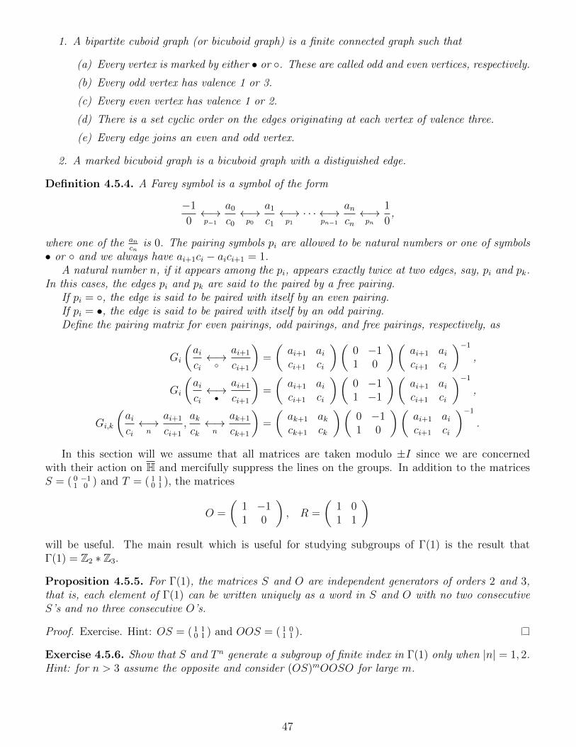
1. A bipartite cuboid graph (or bicuboid graph) is a finite connected graph such that
(a) Every vertex is marked by either • or . These are called odd and even vertices, respectively.
(b) Every odd vertex has valence 1 or 3.
(c) Every even vertex has valence 1 or 2.
(d) There is a set cyclic order on the edges originating at each vertex of valence three.
(e) Every edge joins an even and odd vertex.
2. A marked bicuboid graph is a bicuboid graph with a distiguished edge.
Definition 4.5.4. A Farey symbol is a symbol of the form
−1
0←→p−1
a0
c0
←→p0
a1
c1
←→p1
· · · ←→pn−1
ancn←→pn
1
0,
where one of the ancn
is 0. The pairing symbols pi are allowed to be natural numbers or one of symbols• or and we always have ai+1ci − aici+1 = 1.
A natural number n, if it appears among the pi, appears exactly twice at two edges, say, pi and pk.In this cases, the edges pi and pk are said to the paired by a free pairing.
If pi = , the edge is said to be paired with itself by an even pairing.If pi = •, the edge is said to be paired with itself by an odd pairing.Define the pairing matrix for even pairings, odd pairings, and free pairings, respectively, as
Gi
(aici←→
ai+1
ci+1
)=
(ai+1 aici+1 ci
)(0 −11 0
)(ai+1 aici+1 ci
)−1
,
Gi
(aici←→•
ai+1
ci+1
)=
(ai+1 aici+1 ci
)(0 −11 −1
)(ai+1 aici+1 ci
)−1
,
Gi,k
(aici←→n
ai+1
ci+1
,akck←→n
ak+1
ck+1
)=
(ak+1 akck+1 ck
)(0 −11 0
)(ai+1 aici+1 ci
)−1
.
In this section will we assume that all matrices are taken modulo ±I since we are concernedwith their action on H and mercifully suppress the lines on the groups. In addition to the matricesS = ( 0 −1
1 0 ) and T = ( 1 10 1 ), the matrices
O =
(1 −11 0
), R =
(1 01 1
)will be useful. The main result which is useful for studying subgroups of Γ(1) is the result thatΓ(1) = Z2 ∗ Z3.
Proposition 4.5.5. For Γ(1), the matrices S and O are independent generators of orders 2 and 3,that is, each element of Γ(1) can be written uniquely as a word in S and O with no two consecutiveS’s and no three consecutive O’s.
Proof. Exercise. Hint: OS = ( 1 10 1 ) and OOS = ( 1 0
1 1 ).
Exercise 4.5.6. Show that S and T n generate a subgroup of finite index in Γ(1) only when |n| = 1, 2.Hint: for n > 3 assume the opposite and consider (OS)mOOSO for large m.
47
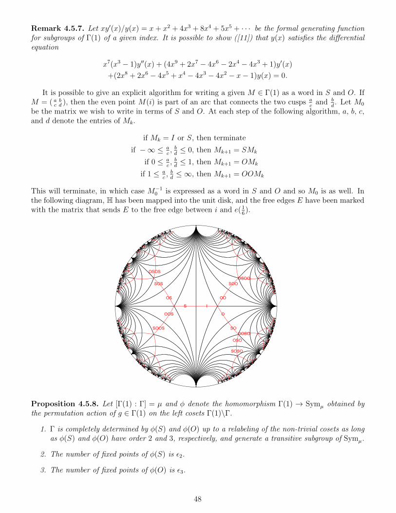
Remark 4.5.7. Let xy′(x)/y(x) = x+ x2 + 4x3 + 8x4 + 5x5 + · · · be the formal generating functionfor subgroups of Γ(1) of a given index. It is possible to show ([11]) that y(x) satisfies the differentialequation
x7(x3 − 1)y′′(x) + (4x9 + 2x7 − 4x6 − 2x4 − 4x3 + 1)y′(x)
+(2x8 + 2x6 − 4x5 + x4 − 4x3 − 4x2 − x− 1)y(x) = 0.
It is possible to give an explicit algorithm for writing a given M ∈ Γ(1) as a word in S and O. IfM = ( a bc d ), then the even point M(i) is part of an arc that connects the two cusps a
cand b
d. Let M0
be the matrix we wish to write in terms of S and O. At each step of the following algorithm, a, b, c,and d denote the entries of Mk.
if Mk = I or S, then terminate
if −∞ ≤ ac, bd≤ 0, then Mk+1 = SMk
if 0 ≤ ac, bd≤ 1, then Mk+1 = OMk
if 1 ≤ ac, bd≤ ∞, then Mk+1 = OOMk
This will terminate, in which case M−10 is expressed as a word in S and O and so M0 is as well. In
the following diagram, H has been mapped into the unit disk, and the free edges E have been markedwith the matrix that sends E to the free edge between i and e(1
6).
IS
O
OOOS
OOS
SO
SOOSOS
OSO
OSOO
SOOSOOSO
OSOS
SOSO
Proposition 4.5.8. Let [Γ(1) : Γ] = µ and φ denote the homomorphism Γ(1) → Symµ obtained bythe permutation action of g ∈ Γ(1) on the left cosets Γ(1)\Γ.
1. Γ is completely determined by φ(S) and φ(O) up to a relabeling of the non-trivial cosets as longas φ(S) and φ(O) have order 2 and 3, respectively, and generate a transitive subgroup of Symµ.
2. The number of fixed points of φ(S) is ε2.
3. The number of fixed points of φ(O) is ε3.
48
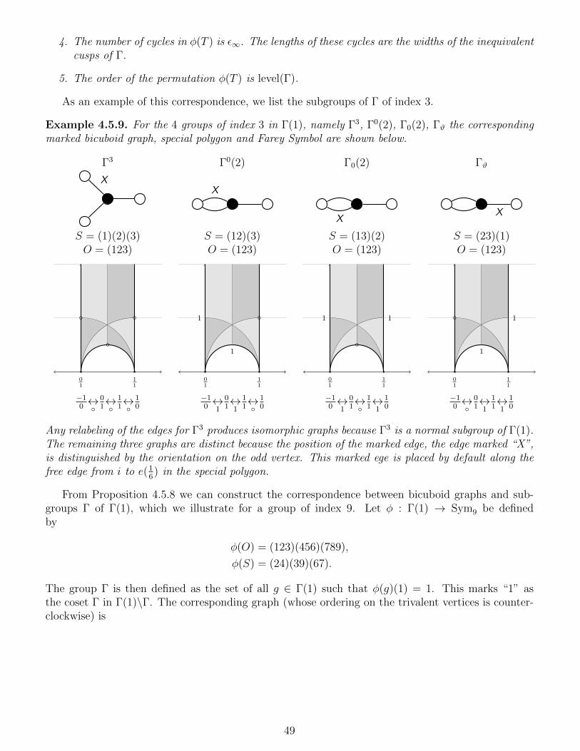
4. The number of cycles in φ(T ) is ε∞. The lengths of these cycles are the widths of the inequivalentcusps of Γ.
5. The order of the permutation φ(T ) is level(Γ).
As an example of this correspondence, we list the subgroups of Γ of index 3.
Example 4.5.9. For the 4 groups of index 3 in Γ(1), namely Γ3, Γ0(2), Γ0(2), Γϑ the correspondingmarked bicuboid graph, special polygon and Farey Symbol are shown below.
Γ3 Γ0(2) Γ0(2) Γϑ
X
S = (1)(2)(3)O = (123)
X
S = (12)(3)O = (123)
X
S = (13)(2)O = (123)
X
S = (23)(1)O = (123)
01
11
1
1
01
11
1 1
01
11
1
1
01
11
−10↔
01↔
11↔
10
−10↔1
01↔1
11↔
10
−10↔1
01↔
11↔1
10
−10↔
01↔1
11↔1
10
Any relabeling of the edges for Γ3 produces isomorphic graphs because Γ3 is a normal subgroup of Γ(1).The remaining three graphs are distinct because the position of the marked edge, the edge marked “X”,is distinguished by the orientation on the odd vertex. This marked ege is placed by default along thefree edge from i to e(1
6) in the special polygon.
From Proposition 4.5.8 we can construct the correspondence between bicuboid graphs and sub-groups Γ of Γ(1), which we illustrate for a group of index 9. Let φ : Γ(1) → Sym9 be definedby
φ(O) = (123)(456)(789),
φ(S) = (24)(39)(67).
The group Γ is then defined as the set of all g ∈ Γ(1) such that φ(g)(1) = 1. This marks “1” asthe coset Γ in Γ(1)\Γ. The corresponding graph (whose ordering on the trivalent vertices is counter-clockwise) is
49
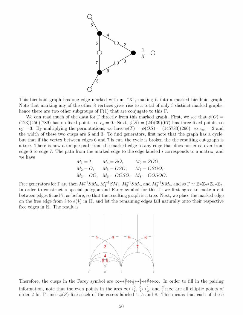
1
5
8
2
4
3
9
6
7
X
This bicuboid graph has one edge marked with an “X”, making it into a marked bicuboid graph.Note that marking any of the other 8 vertices gives rise to a total of only 3 distinct marked graphs,hence there are two other subgroups of Γ(1) that are conjugate to this Γ.
We can read much of the data for Γ directly from this marked graph. First, we see that φ(O) =(123)(456)(789) has no fixed points, so ε3 = 0. Next, φ(S) = (24)(39)(67) has three fixed points, soε2 = 3. By multiplying the permutations, we have φ(T ) = φ(OS) = (145783)(296), so ε∞ = 2 andthe width of these two cusps are 6 and 3. To find generators, first note that the graph has a cycle,but that if the vertex between edges 6 and 7 is cut, the cycle is broken the the resulting cut graph isa tree. There is now a unique path from the marked edge to any edge that does not cross over fromedge 6 to edge 7. The path from the marked edge to the edge labeled i corresponds to a matrix, andwe have
M1 = I, M4 = SO, M9 = SOO,
M2 = O, M5 = OSO, M7 = OSOO,
M3 = OO, M6 = OOSO, M8 = OOSOO.
Free generators for Γ are thenM−17 SM6, M−1
1 SM1, M−15 SM5, andM−1
8 SM8, and so Γ ' Z∗Z2∗Z2∗Z2.In order to construct a special polygon and Farey symbol for this Γ, we first agree to make a cutbetween edges 6 and 7, as before, so that the resulting graph is a tree. Next, we place the marked edgeon the free edge from i to e(1
6) in H, and let the remaining edges fall naturally onto their respective
free edges in H. The result is
1
2
3 9
7
8
45 6
0 12 1 2
Therefore, the cusps in the Farey symbol are ∞↔01↔1
2↔1
1↔2
1↔∞. In order to fill in the pairing
information, note that the even points in the arcs ∞↔01, 0
1↔1
2, and 2
1↔∞ are all elliptic points of
order 2 for Γ since φ(S) fixes each of the cosets labeled 1, 5 and 8. This means that each of these
50
three arcs is paired with itself. Finally the arc 12↔1
1is paired with the arc 1
1↔2
1in order to glue back
together the cut that was made between the edges 6 and 7. In summary, a Farey symbol for Γ isgiven by
∞←→
0
1←→
1
2←→
1
1
1←→
1
2
1←→∞.
We could have made one cut between edges 2 and 4 or 3 and 9, so there are in total two more Fareysymbols corresponding to this subgroup Γ.
Algorithm 4.5.10. Input: a finite index subgroup Γ of Γ(1). Output: a Farey symbol for Γ.Step 1: If [Γ(1) : Γ] ≤ 2
return
−10←→
01←→•
10
, ( 0 −11 0 ), ( 1 1
0 1 ) ∈ Γ (i.e. Γ = Γ(1))
−10←→•
01←→•
10
, ( 0 −11 1 ), ( 1 −1
0 1 ) ∈ Γ (i.e. Γ = Γ2).
Step 2: Let F be the partial Farey symbol
F =
−10←→ 0
1←→ 1
1←→ 1
0, ( 1 −1
1 0 ) 6∈ Γ
−10←→ −1
1←→ 0
1←→ 1
0, ( 1 −1
1 0 ) ∈ Γ.
Step 3: For each unpaired edge in F , check if it can be paired with itself by an even or odd pairing(Gi ∈ Γ) or if it can be paired with another unpaired edge (free pairing Gi,k ∈ Γ) and fill in all of thepossible pairings.Step 4: If all edges are paired, then return F .Step 5: If there is still an unpaired edge in F between, say, ai/ci and ai+1/ci+1, place an new vertex(ai + ai+1)/(ci + ci+1) in between with no pairing information on the two adjacent edges and goto Step3.
Given a special polygon P , we may convert P to a Farey symbol F and vice-versa. If P is a specialpolygon, we assume that that ∞ is included as a vertex and that there are certain rational verticesa0
c0< · · · < an
cn. These are put into F in the obvious way with the corresponding pairing information.
Note that we have ai+1ci − aici+1 = 1 because the quantity ai+1ci − aici+1 is unchanged when aici
andai+1
ci+1are simultaneously acted upon by some element of Γ(1) and ai+1ci − aici+1 = 1 for the basic
choices aici
= −10
and ai+1
ci+1= 0
1.
Now given F , we can convert to edges of P in the following way (set g = ( ai+1 aici+1 ci )).
aici←→
ai+1
ci+1
aici←→n
ai+1
ci+1
⇐⇒ g(E ∪ ( 0 −1
1 0 )(l)), E = e(14) + it | t > 0
aici←→•
ai+1
ci+1
⇐⇒ g(E ∪ ( 0 −11 −1 )(E)), E = e(1
6) + it | t > 0
Theorem 4.5.11.
1. If P is a special polygon, then the edge pairing matrices gi generate some Γ and P is afundamental domain for Γ.There are ε2 generators of order 2.There are ε3 generators of order 3.There are 2g + ε∞ − 1 free generators (order ∞).
51
2. The gi are an independent set of generators for Γ. This means that any element of Γ can bewritten uniquely as
∏gk∈gi g
ekk where ek 6= 0 and ek is further restricted to 1 ≤ ek < p if gk is
a generator of finite order p. In symbols,
Γ ' Z∗ε22 ∗ Z∗ε33 ∗ Z∗(2g−1+ε∞).
Proof. See [9].
4.6 Γ(2)
The main function for the group Γ(2), which play the same role as j(τ) plays for Γ(1) (the so-calledHauptmodul), is the modular λ function defined by
λ(τ) =
(Θ2(τ)
Θ3(τ)
)4
.
Proposition 4.6.1. Let λ(τ) be the modular λ function. Then,
1. λ(τ) ∈M !0(Γ(2)), Θ4
2,Θ43,Θ
44 ∈M2(Γ(2))
2. λ(τ) has a simple pole at 11, a simple zero at 1
0, and takes the value 1 at 0
1.
3. A0(Γ(2)) = C(λ).
4. Sk(Γ(2)) = Θ42Θ4
3Θ44Mk−6(Γ(2)).
5. Θ43 = Θ4
2 + Θ44.
6. Mk(Γ(2)) =⊕
2a+2b=ka,b≥0
CΘ4a2 Θ4b
3 .
Proof. (1). The fundamental domain τ | |Re(τ)| ≤ 1 and |2τ ± 1| ≥ 1 for Γ(2) shows that Γ(2) isgenerated by T 2 and ST 2S. From Proposition 2.8.3, we have
(Θ2,Θ3,Θ4)|T = (ζ18Θ2,Θ3,Θ4),
(Θ2,Θ3,Θ4)|S = ζ−18 (Θ4,Θ3,Θ2).
Therefore,
(Θ2,Θ3,Θ4)|T 2 = (ζ4Θ2,Θ3,Θ4),
(Θ2,Θ3,Θ4)|ST 2S = (ζ34Θ2, ζ
34Θ3,Θ4).
and we see that Θ42/Θ
43 ∈M !
0(Γ(2)) because Exercise 2.12.4 shows that λ has no poles or zeros in H.(2). For the values at the cusps, we have the table
cusp function q-series10
λ|I Θ42
Θ43
= 2q1/2 + · · ·01
λ|S Θ44
Θ43
= 1 + · · ·11
λ|TS −Θ44
Θ42
= −12q−1/2 + · · ·
52
(3). Since ordΓ(2)(λ) = 1 all of the assertions of Proposition 4.4.7 apply.(4). Since Θ4
2Θ43Θ4
4 has a simple zero at each cusp, we must obtain Sk in this way.(5). The form Θ4
2 + Θ44 − Θ4
3 = O(q2/2) in M2(Γ(2)) has a zero of order at least 2 at ∞ whichcontradicts the valence formula unless this function vanishes identically.
(6). First note Θ2 and Θ3 are algebraically independent. If f ∈ Mk(Γ(2)) with k ≥ 0 and even,then g := f/Θ2k
3 ∈ A0(Γ(2)) with the only possible pole of g located at the pole of λ. Therefore,part 2 of Prop 4.4.7 shows that g is a polynomial in λ of degree no more than k/2 since the valenceformula says that f has k/2 zeros (hence g has no more than k/2 zeros).
4.7 Building congruence modular forms N from Klein Forms
A subgroup Γ of Γ(1) is called a congruence subgroup if Γ contains Γ(N) for some N . The smallestsuch N turns out to be the level of Γ in this case (see Proposition 4.13.4 below). Similarly, a modularfunction f is said to have level N if it is invariant under Γ(N). Most subgroups of Γ(1) are notcongruence; let an denote the number of subgroups of Γ(1) of index n and let bn denote the numberof congruence subgroups of Γ(1) of index at most n. Then it is known ([11], [12], [15]) that
an ∼ exp
(1
6n log n− 1
6n+ n1/2 + n1/3 +
1
2log n− 1
4− 1
2log 2π
),
log(bn) ∼
(√2− 1
2
)2log2 n
log log n.
One of the building blocks of modular forms of higher levels is the Klein form k~r(τ), which isdefined for ~r ∈ Q2, τ ∈ H and has weight −1 and generalizes η(τ)−2. We will also introduce a form ofpositive integral weight k by ek~r(τ) which generalizes the Eisenstein series E2k(τ). Set
k~r(τ) = −2πizeπir1z∏ω∈Λ′
(1 +
z
ω
)e−
zω ,
e1~r(τ) =
1
2πi
(1
z+∑Ω∈Λ′
1
z + ω− 1
ω
),
ek~r(τ) =(k − 1)!
(2πi)k
∑ω∈Λ
1
(z + ω)k, k ≥ 2,
where Λ = Zτ +Z and z = r1τ + r2 and the sums or products over ω = mτ + n are performed over nfirst and then m. These sums are not defined if ~r ∈ Z2, in which we take out the undefined term andobtain the definitions
ek~r(τ) =
ζ(1− k)Ek(τ) , k even
0 , k odd, for ~r ∈ Z2.
53
Proposition 4.7.1. Set z = r1τ + r2. The Klein forms have the series expansions,
k~r(τ) = q(r1−1)/2z
(qz; q)∞(q/qz; q)∞(q; q)2
∞,
e1~r(τ) =
qz + 1
2(qz − 1)−∞∑n=1
(qnz − q−nz )qn
1− qn, for |r1| < 1,
e2~r(τ) =
qz(qz − 1)2
+∞∑n=1
(qnz + q−nz )nqn
1− qn, for |r1| < 1,
e3~r(τ) =
qz(qz + 1)
(qz − 1)3−∞∑n=1
(qnz − q−nz )n2qn
1− qn, for |r1| < 1,
where ek+1~r (τ) is formally obtained from ek~r(τ) by applying −1
2πi∂∂z
.
Proposition 4.7.2. For N > 1, we have
N−1∏j=0
k iN, jN
(τ) = ζ(N−1)(i−N)4N
η(Nτ)2
η(τ)2Nk iN, 0N
(Nτ),
N−1∏j=1
k 0N, jN
(τ) = ζ1−N4
η(Nτ)2
η(τ)2N.
Proposition 4.7.3. For ~r = (r1, r2) and g = ( a bc d ) ∈ Γ(1),
k~r|g(τ) = k~r.g(τ),
e1~r|g(τ) = e1
~r.g(τ) + c(aτ + b)r1 + c(cτ + d)r2,
e2~r|g(τ) = e2
~r.g(τ)− c
2πi(cτ + d),
ek~r |g(τ) = ek~r.g(τ), k ≥ 3.
If (n1, n2) ∈ Z2,
k~r+(n1,n2)(τ) = (−1)n1+n2+n1n2e(12(r1n2 − r2n1))k~r(τ),
e1~r+(n1,n2)(τ) = e1
~r(τ)− n1,
ek~r+(n1,n2)(τ) = ek~r(τ), k ≥ 2.
Proposition 4.7.4. If gcd(a, c) = 1, then
ordack~r(τ) =
(frac(~r.~v)
2
),
where ~v = (a, c)ᵀ is the vector corresponding to the cusp ac
and frac(x) denotes the fractional part ofx that satisfies 0 ≤ frac(x) < 1.
Proof. Exercise.
Proposition 4.7.5. For ~r = (r1, r2) ∈ 1NZ2,
54
1. For k = −∑
~rm(~r), the form∏~r k~r(τ)m(~r) is in M !
k(Γ(N)) if and only if∑~r
m(~r)(Nr1)2 ≡ 0 mod N gcd(2, N),∑~r
m(~r)(Nr2)2 ≡ 0 mod N gcd(2, N),∑~r
m(~r)(Nr1)(Nr2) ≡ 0 mod N .
2. The form∑
~rm(~r)e1~r(τ) is in M1(Γ(N)) if and only if
∑~rm(~r)r1 = 0.
3. The form∑
~rm(~r)e2~r(τ) is in M2(Γ(N)) if and only if
∑~rm(~r) = 0.
4. The form∑
~rm(~r)ek~r(τ) is in Mk(Γ(N)) for any k ≥ 3.
We will give a generator xN for the function field A0(Γ(N)) for N < 6 in Section 4.9. The followingtheorem tells us that two ratios of Klein forms suffice for N ≥ 6.
Theorem 4.7.6 ([7]). For N ≥ 6, we have A0(Γ(N)) = C(x2,N(τ), x3,N(τ)), where
xr,N(τ) =
(kr/N,0(Nτ)
k1/N,0(Nτ)
)gcd(2,r,N)
.
Furthermore, x3,N is integral over Q[x2,N ].
4.8 Building congruence modular forms from η products
Proposition 4.8.1. Let gcd(a, c) = 1 and M ∈ Z2×2 with detM > 0. Then,
ordacη|M(τ) =
1
24
gcd(M.~v)2
det(M),
where ~v = (a, c)ᵀ is the vector corresponding to the cusp ac.
Proof. Exercise.
Proposition 4.8.2. Set Γ = Γ0(N) and suppose that f(τ) =∏
l|N η(lτ)rl and that the three numbers
k = 12
∑l|N
rl, ord∞(f,Γ) = 124
∑l|N
lrl, ord0(f,Γ) = 124
∑l|N
Nlrl,
are all integers. Then, for any g = ( a bc d ) ∈ Γ with odd d, f satisfies
f |g,k(τ) =
((−1)k
∏l|N l
|rl|
d
)f(τ).
Remark 4.8.3. In the case that d is even, c must be odd and we can recover the multiplier for suchd by
f |g,k(τ) =
((−1)k
∏l|N l
|rl|
c+ d
)f(τ).
simply be replacing τ by τ − 1.
55
Proof. Assuming d is odd, the multiplier system for η (Exercise 2.12.6) has the form
η
(aτ + b
cτ + d
)=
(c
|d|
)ζ
3d+d(b−c)+ac(1−d2)24
√−i(cτ + d)η(τ),
or η
(laτ + b
cτ + d
)rl=
(c|rl|l|rl|
|d|
)ζ
3drl+dblrl−(ad2−a+d) cNNlrl
24 (−i(cτ + d))rl2 η(lτ)rl ,
since l aτ+bcτ+d
= a(lτ)+blcNNl
(lτ)+d. Therefore
f |g,k(τ)
f(τ)= (−i)k
(c2|k|∏
l|N l|rl|
|d|
)ζ
6dk+24db ord∞(f,Γ)−24(ad2−a+d) cN
ord0(f,Γ)
24
=
((−1)k
∏l|N l
|rl|
d
),
since k, ord∞(f,Γ), and ord0(f,Γ) are all integers.
Following [6], the η function can be generalized to any even real Dirichlet character χ. Set
ηχ(τ) = q−12L(−1,χ)
∞∏n=1
(1− qn)χ(n), (χ(−1) = 1).
Here L(s, χ) is the Dirichlet series∑∞
n=1χ(n)ns
, which converges for s > 1 and can be analyticallycontinued to C with a possible pole at s = 1. When χ is the function 1 identically, we recoverthe usual η function because of the value L(−1, 1) = ζ(−1) = − 1
12. It suffices to study primitive
characters because if χ is a character modulo k and χ(n) = χ1(n)χ0(n) where χ1 is the primitivecharacter modulo ∆|k and χ0(n) is the principle character modulo k, then
ηχ(τ) =∏l| k
∆
ηχ1(lτ)µ(l)χ1(l).
It should be pointed out at this point that the only real even primitive characters are given by
χ(n) =
(∆
n
),
where( ··
)is the Kronecker symbol and ∆ is a fundamental discriminant (see definition 7.3.1). The
period of this character is ∆.
Proposition 4.8.4 ([6]). Let ∆ > 1 be a fundamental discriminant and χ the associated primitive realeven character. Set χ′(n) to be χ(n) if ∆ is a prime, and 1 otherwise. Then, for any ( a bc d ) ∈ Γ0(∆),ηχ satisfies the transformation formula
ηχ
(aτ + b
cτ + d
)= χ′(d)ηχ(τ)χ(d) ×
ζab5 , ∆ = 5
ζa−d+bc−8b16 , ∆ = 8
1 , ∆ > 8
.
56
4.9 Γ(N) and regular polyhedron
It is known that the finite groups acting faithfully on C∞ are exactly
Zn the cyclic group of order n,Zn o Z2 the dihedral group of order 2n,A4 the symmetries of the tetrahedron of order 12,S4 the symmetries of the octahedron of order 24,A5 the symmetries of the icosahedron of order 60.
For the modular group, it turns out that restricting to normal subgroups of genus 0 puts a restrictionon the first two types, and there is a finite list of possible groups. First, for any subgroup Γ withµ = [Γ(1) : Γ], let e2 (resp. e3, e∞) denote the number of equivalent classes under Γ of the pointsΓ(1)(i) (resp. Γ(1)(e(1
3)), Γ(1)(∞)). Thus, em = εm + µ−εm
mfor m = 2, 3,∞ since e∞ = ε∞. Next,
suppose that Γ is a normal subgroup of Γ(1). This means that the order of any point is same, andtherefore that em|µ for m = 2, 3,∞. Thus, in this case we can define nm by
µ = n2e2 = n3e3 = n∞e∞,
and this corresponds to the triplet (n2, n3, n∞) describing the branching information of Γ. The genusformula may be rearranged as
2− 2g
µ=
1
n2
+1
n3
+1
n∞− 1. (4.9.1)
Note that n2 is either 1 or 2 and n3 is either 1 or 3, while n∞, which is the width of any cusp, hasno such restriction. An easy consequence is that µ ≡ 0 mod 6 if µ > 3. Also, if Γ2 E Γ1 E Γ(1), theneach nm(Γ1) divides nm(Γ2).
Proposition 4.9.1. If Γ is a proper normal subgroup of Γ(1) with finite index and genus 0, then Γis one of the following:
Γ Γ(1)/Γ Γ Γ(1)/ΓΓ2 Z2 Γ(3) A4
Γ3 Z3 Γ(4) S4
Γ(2) S3 ' Z3 o Z2 Γ(5) A5
Proof. We first deal with the case n2 = n3 = 1. In this case, (4.9.1) is 2µ
= 1+ 1n∞
and so µ = 1 = n∞.
So in this case, Γ = Γ(1). Next, suppose that n2 = 1 and n3 = 3, so that 2µ
= 13
+ 1n∞
. Since µ ≥ n∞this implies that µ = 3 and that Γ = Γ3 as this is the only normal subgroup of index 3. Next, supposethat n2 = 2 and n3 = 1, so that 2
µ= 1
2+ 1
n∞. Since µ ≥ n∞ this implies that µ = 2 and that Γ = Γ2
as this is the only normal subgroup of index 2. Next, suppose that n2 = 2 and n3 = 3, so that2µ
= −16
+ 1n∞
. This implies that n∞ = 2, 3, 4, 5 with corresponding µ = 6, 12, 24, 60. Set G = Γ(1)/Γ
so that µ = |G|. We will first determine G up to isomorphism and then Γ exactly. Note that G isgenerated (modulo Γ) by S, ST and T with S2 = (ST )3 = T n∞ = 1.
First, suppose that |G| = 6, (2, 3, 2). Since S has order 2 and ST has order 3 but their product Thas order 2 (not 6), G cannot be Abelian, and so G ' S3.
Next, suppose that |G| = 12, (2, 3, 3). A Sylow 3 subgroup cannot be normal, because otherwiseits quotient would correspond to a normal subgroup of Γ(1) of index 4 which doesn’t exist. Since A4
is the only group of order 12 that doesn’t have a normal Sylow 3 subgroup, G ' A4.Next, suppose that |G| = 24, (2, 3, 4). As before, there are 4 Sylow 3 subgroups, and we obtain a
homomorphism φ : G→ S4 by the action of G on the 4 Sylow 3 subgroups where imφ ' A4, S4 sincethese are the only transitive subgroups of S4 whose order is divisible by 6. If imφ = A4, then this
57
corresponds to another normal subgroup Γ1 of index 12. The only group with index 12 correspondsto the triplet (2, 3, 3), which does not divide the triplet (2, 3, 4). Hence imφ = S4 and so G ' S4.
Finally, suppose that |G| = 60, (2, 3, 5). Since the only triplets dividing (2, 3, 5) are the trivialones, G must be simple. Standard group theory arguments using the Sylow 2 subgroup show that A5
is the only simple group of order 60.To finish the proof, we need to show that Γ(N) is the only possibility for Γ when the branching
information is (2, 3, N) (and g = 0). By Proposition 4.3.1, the groups Γ(2),Γ(3),Γ(4),Γ(5) have thecorrect indexes in Γ(1), that is
µ =12N
6−N= [Γ(1) : Γ(N)] =
12N3∏
p|N
(1− 1
p2
), N ≥ 3
6 , N = 2,
for N = 2, 3, 4, 5. Consider Γ∩Γ(N) for N = 2, 3, 4, 5. We know that Γ∩Γ(N) is a normal subgroupof Γ, but be do not know a priori that the genus of Γ ∩ Γ(N) is 0. However, we are given that bothΓ and Γ(N) have cusp width N , and so Γ ∩ Γ(N) has cusp width N . This means that the branchingdata of Γ ∩ Γ(N) is (2, 3, N) and if µ and g denote the index and genus of Γ ∩ Γ(N), we have
2− 2g
µ=
1
2+
1
3+
1
N− 1.
Since the right hand side is strictly positive for N = 2, 3, 4, 5, g is forced to be 0 and µ is forced to be12N/(6−N). This means that [Γ(1) : Γ ∩ Γ(N)] = [Γ(1) : Γ(N)], which forces Γ = Γ(N).
Although we deduced that there is only one normal subgroup of genus 0 with branching data(2, 3, N) for N = 2, 3, 4, 5, this result does not need to hold for higher genera. For example, all normalsubgroups of genus 1 have branching data (2, 3, 6), and there are infinitely many of them ([13]).
Having classified all of the normal subgroup Γ of Γ(1) with genus 0, let us turn now to theproblem of constructing the spaces Mk(Γ) for these Γ. The groups Γ2 and Γ3 are not very interesting,as (Exercise 4.9.8)
A0(Γ2) = C(√j − 1728), A0(Γ3) = C(j1/3).
so let us turn to Γ(N) for N = 2, 3, 4, 5. Assuming that there is a Hauptmodul, say fN(τ), for theseΓ(N), it is possible to show that there is a Hauptmodul xN that is uniquely determined by
xN(τ) = q−1N (1 + integral powers of q).
Since Γ(N) is a normal subgroup of Γ(1), there must be constants A,B,C,D, depending on N , suchthat
fN |T =AfN +B
CfN +D.
By rescaling the matrix M = ( A BC D ), we may assume that one of its eigenvalues is 1. If the other
eigenvalue were 1, then ( A BC D ) would be similar to either ( 1 1
0 1 ) or ( 1 00 1 ). The first is a contradiction
because MN
= I since TN ∈ Γ(N). If the second were true then fN would be invariant under T andso N divides ord∞(fN(τ) − fN(∞),Γ(N)) 6= 0, which is a contradiction because fN(τ) − fN(∞) isalso a Hauptmodul for Γ(N). We now have M = P−1( ζ 0
0 1 )P where ζ is an N th root of unity. SettingxN = P (fN) gives xN |T = ζrNxN for some integer r and so q−r/NxN has an expansion in integralpowers of q. Since xN is also a Hauptmodul, r = ±1 and we choose r = −1 whicn gives xN a simple
58
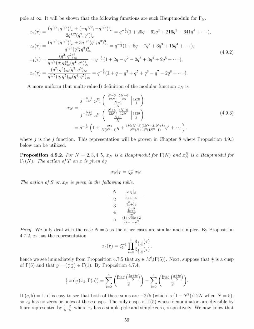
pole at ∞. It will be shown that the following functions are such Hauptmoduln for ΓN .
x2(τ) =(q1/2; q1/2)8
∞ + (−q1/2;−q1/2)8∞
2q1/2(q2; q2)8∞
= q−12 (1 + 20q − 62q2 + 216q3 − 641q4 + · · · ),
x3(τ) =(q1/3; q1/3)3
∞ + 3q1/3(q3; q3)3∞
q1/3(q3; q3)3∞
= q−13 (1 + 5q − 7q2 + 3q3 + 15q4 + · · · ),
x4(τ) =(q2; q2)6
∞q1/4(q; q)2
∞(q4; q4)4∞
= q−14 (1 + 2q − q2 − 2q3 + 3q4 + 2q5 + · · · ),
x5(τ) =(q2; q5)∞(q3; q5)∞q1/5(q; q5)∞(q4; q5)∞
= q−15 (1 + q − q3 + q5 + q6 − q7 − 2q8 + · · · ).
(4.9.2)
A more uniform (but multi-valued) definition of the modular function xN is
xN =
j−N−612N 2F1
( N−612N
, 5N−612N
N−1N
∣∣∣1728j
)j−
N+612N 2F1
( N+612N
, 5N+612N
N+1N
∣∣∣1728j
)= q−
1N
(1 + 120
N(N2−1)q + 180(N−5)(3N2+21N+8)
N2(N+1)2(4N2−1)q2 + · · ·
),
(4.9.3)
where j is the j function. This representation will be proven in Chapter 8 where Proposition 4.9.3below can be utilized.
Proposition 4.9.2. For N = 2, 3, 4, 5, xN is a Hauptmodul for Γ(N) and xNN is a Hauptmodul forΓ1(N). The action of T on x is given by
xN |T = ζ−1N xN .
The action of S on xN is given in the following table.
N xN |S2 8x+192
x−1
3 3x+18x−3
4 2x+4x−2
5 (1+√
5)x+2
2x−1−√
5
Proof. We only deal with the case N = 5 as the other cases are similar and simpler. By Proposition4.7.2, x5 has the representation
x5(τ) = ζ−15
4∏i=0
k 25, i5(τ)
k 15, i5(τ)
,
hence we see immediately from Proposition 4.7.5 that x5 ∈M !0(Γ(5)). Next, suppose that a
cis a cusp
of Γ(5) and that g = ( a bc d ) ∈ Γ(1). By Proposition 4.7.4,
15
ordac(x5,Γ(5)) =
4∑i=0
(frac
(2a+ic
5
)2
)−
4∑i=0
(frac
(a+ic
5
)2
).
If (c, 5) = 1, it is easy to see that both of these sums are −2/5 (which is (1−N2)/12N when N = 5),so x5 has no zeros or poles at these cusps. The only cusps of Γ(5) whose denominators are divisible by5 are represented by 1
5, 2
5, where x5 has a simple pole and simple zero, respectively. We now know that
59
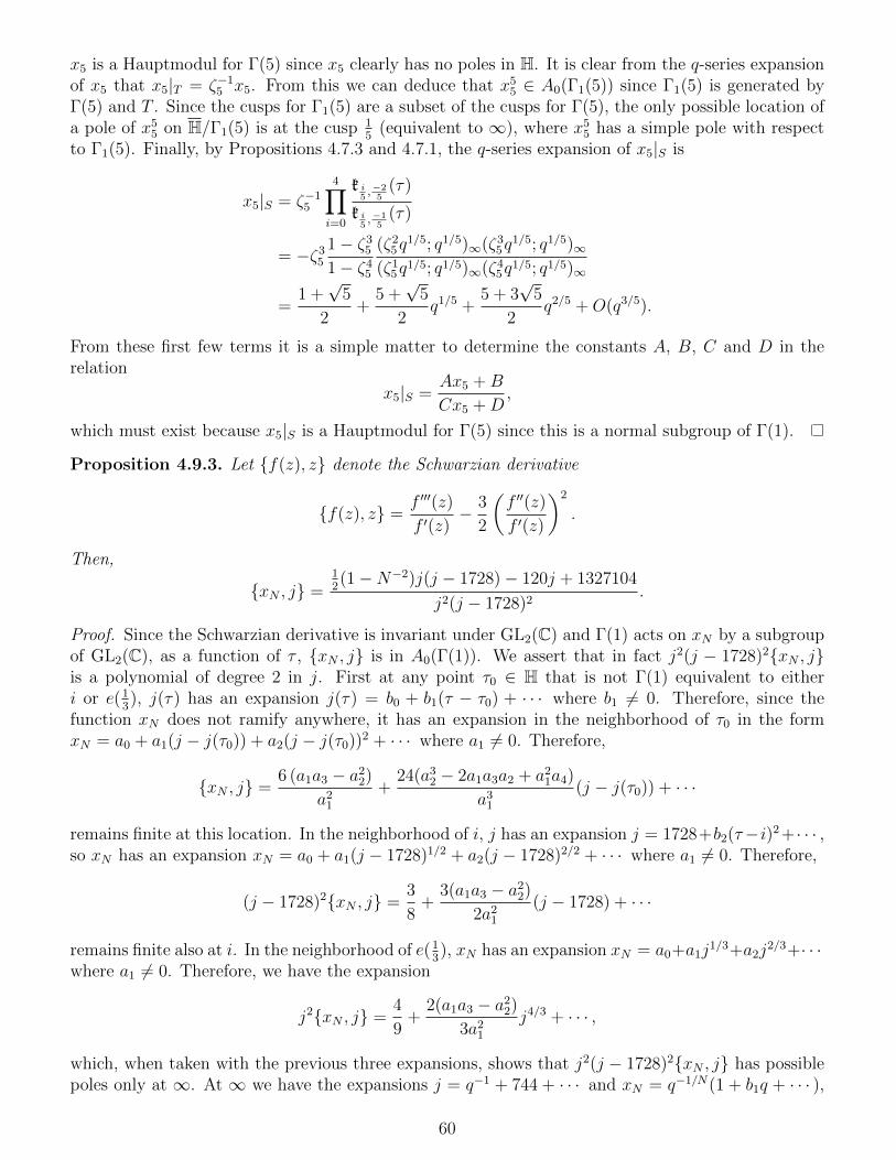
x5 is a Hauptmodul for Γ(5) since x5 clearly has no poles in H. It is clear from the q-series expansionof x5 that x5|T = ζ−1
5 x5. From this we can deduce that x55 ∈ A0(Γ1(5)) since Γ1(5) is generated by
Γ(5) and T . Since the cusps for Γ1(5) are a subset of the cusps for Γ(5), the only possible location ofa pole of x5
5 on H/Γ1(5) is at the cusp 15
(equivalent to ∞), where x55 has a simple pole with respect
to Γ1(5). Finally, by Propositions 4.7.3 and 4.7.1, the q-series expansion of x5|S is
x5|S = ζ−15
4∏i=0
k i5,−2
5(τ)
k i5,−1
5(τ)
= −ζ35
1− ζ35
1− ζ45
(ζ25q
1/5; q1/5)∞(ζ35q
1/5; q1/5)∞(ζ1
5q1/5; q1/5)∞(ζ4
5q1/5; q1/5)∞
=1 +√
5
2+
5 +√
5
2q1/5 +
5 + 3√
5
2q2/5 +O(q3/5).
From these first few terms it is a simple matter to determine the constants A, B, C and D in therelation
x5|S =Ax5 +B
Cx5 +D,
which must exist because x5|S is a Hauptmodul for Γ(5) since this is a normal subgroup of Γ(1).
Proposition 4.9.3. Let f(z), z denote the Schwarzian derivative
f(z), z =f ′′′(z)
f ′(z)− 3
2
(f ′′(z)
f ′(z)
)2
.
Then,
xN , j =12(1−N−2)j(j − 1728)− 120j + 1327104
j2(j − 1728)2.
Proof. Since the Schwarzian derivative is invariant under GL2(C) and Γ(1) acts on xN by a subgroupof GL2(C), as a function of τ , xN , j is in A0(Γ(1)). We assert that in fact j2(j − 1728)2xN , jis a polynomial of degree 2 in j. First at any point τ0 ∈ H that is not Γ(1) equivalent to eitheri or e(1
3), j(τ) has an expansion j(τ) = b0 + b1(τ − τ0) + · · · where b1 6= 0. Therefore, since the
function xN does not ramify anywhere, it has an expansion in the neighborhood of τ0 in the formxN = a0 + a1(j − j(τ0)) + a2(j − j(τ0))2 + · · · where a1 6= 0. Therefore,
xN , j =6 (a1a3 − a2
2)
a21
+24(a3
2 − 2a1a3a2 + a21a4)
a31
(j − j(τ0)) + · · ·
remains finite at this location. In the neighborhood of i, j has an expansion j = 1728+b2(τ−i)2 + · · · ,so xN has an expansion xN = a0 + a1(j − 1728)1/2 + a2(j − 1728)2/2 + · · · where a1 6= 0. Therefore,
(j − 1728)2xN , j =3
8+
3(a1a3 − a22)
2a21
(j − 1728) + · · ·
remains finite also at i. In the neighborhood of e(13), xN has an expansion xN = a0+a1j
1/3+a2j2/3+· · ·
where a1 6= 0. Therefore, we have the expansion
j2xN , j =4
9+
2(a1a3 − a22)
3a21
j4/3 + · · · ,
which, when taken with the previous three expansions, shows that j2(j − 1728)2xN , j has possiblepoles only at ∞. At ∞ we have the expansions j = q−1 + 744 + · · · and xN = q−1/N(1 + b1q + · · · ),
60
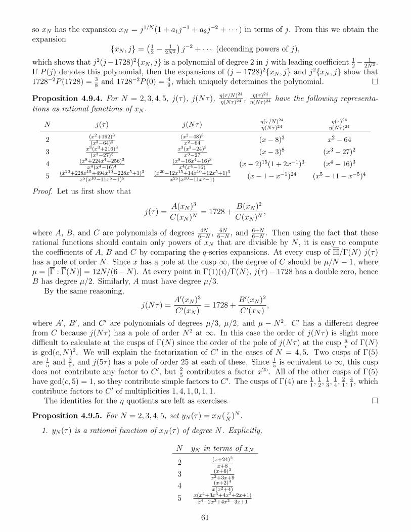
so xN has the expansion xN = j1/N(1 + a1j−1 + a2j
−2 + · · · ) in terms of j. From this we obtain theexpansion
xN , j =(
12− 1
2N2
)j−2 + · · · (decending powers of j),
which shows that j2(j−1728)2xN , j is a polynomial of degree 2 in j with leading coefficient 12− 1
2N2 .If P (j) denotes this polynomial, then the expansions of (j − 1728)2xN , j and j2xN , j show that1728−2P (1728) = 3
8and 1728−2P (0) = 4
9, which uniquely determines the polynomial.
Proposition 4.9.4. For N = 2, 3, 4, 5, j(τ), j(Nτ), η(τ/N)24
η(Nτ)24 , η(τ)24
η(Nτ)24 have the following representa-
tions as rational functions of xN .
N j(τ) j(Nτ) η(τ/N)24
η(Nτ)24η(τ)24
η(Nτ)24
2 (x2+192)3
(x2−64)2(x2−48)3
x2−64(x− 8)3 x2 − 64
3 x3(x3+216)3
(x3−27)3x3(x3−24)3
x3−27(x− 3)8 (x3 − 27)2
4 (x8+224x4+256)3
x4(x4−16)4(x8−16x4+16)3
x4(x4−16)(x− 2)15(1 + 2x−1)3 (x4 − 16)3
5 (x20+228x15+494x10−228x5+1)3
x5(x10−11x5−1)5(x20−12x15+14x10+12x5+1)3
x25(x10−11x5−1)(x− 1− x−1)24 (x5 − 11− x−5)4
Proof. Let us first show that
j(τ) =A(xN)3
C(xN)N= 1728 +
B(xN)2
C(xN)N,
where A, B, and C are polynomials of degrees 4N6−N , 6N
6−N , and 6+N6−N . Then using the fact that these
rational functions should contain only powers of xN that are divisible by N , it is easy to computethe coefficients of A, B and C by comparing the q-series expansions. At every cusp of H/Γ(N) j(τ)has a pole of order N . Since x has a pole at the cusp ∞, the degree of C should be µ/N − 1, whereµ = [Γ : Γ(N)] = 12N/(6−N). At every point in Γ(1)(i)/Γ(N), j(τ)− 1728 has a double zero, henceB has degree µ/2. Similarly, A must have degree µ/3.
By the same reasoning,
j(Nτ) =A′(xN)3
C ′(xN)= 1728 +
B′(xN)2
C ′(xN),
where A′, B′, and C ′ are polynomials of degrees µ/3, µ/2, and µ − N2. C ′ has a different degreefrom C because j(Nτ) has a pole of order N2 at ∞. In this case the order of j(Nτ) is slight moredifficult to calculate at the cusps of Γ(N) since the order of the pole of j(Nτ) at the cusp a
cof Γ(N)
is gcd(c,N)2. We will explain the factorization of C ′ in the cases of N = 4, 5. Two cusps of Γ(5)are 1
5and 2
5, and j(5τ) has a pole of order 25 at each of these. Since 1
5is equivalent to ∞, this cusp
does not contribute any factor to C ′, but 25
contributes a factor x25. All of the other cusps of Γ(5)have gcd(c, 5) = 1, so they contribute simple factors to C ′. The cusps of Γ(4) are 1
1, 1
2, 1
3, 1
4, 2
1, 4
1, which
contribute factors to C ′ of multiplicities 1, 4, 1, 0, 1, 1.The identities for the η quotients are left as exercises.
Proposition 4.9.5. For N = 2, 3, 4, 5, set yN(τ) = xN( τN
)N .
1. yN(τ) is a rational function of xN(τ) of degree N . Explicitly,
N yN in terms of xN
2 (x+24)2
x+8
3 (x+6)3
x2+3x+9
4 (x+2)4
x(x2+4)
5 x(x4+3x3+4x2+2x+1)x4−2x3+4x2−3x+1
61
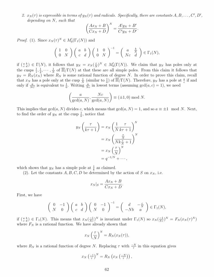
2. xN(τ) is expressible in terms of yN(τ) and radicals. Specifically, there are constants A,B, . . . , C ′, D′,depending on N , such that (
AxN +B
CxN +D
)N=A′yN +B′
C ′yN +D′.
Proof. (1). Since xN(τ)N ∈M !0(Γ1(N)) and(
1 00 N
)(a bc d
)(1 00 N
)−1
=
(a b
N
Nc d
)∈ Γ1(N),
if ( a bc d ) ∈ Γ(N), it follows that yN = xN( τN
)N ∈ M !0(Γ(N)). We claim that yN has poles only at
the cusps 11, 1
2, · · · , 1
Nof H/Γ(N) at that these are all simple poles. From this claim it follows that
yN = RN(xN) where RN is some rational function of degree N . In order to prove this claim, recallthat xN has a pole only at the cusp 1
N(similar to 1
0) of H/Γ(N). Therefore, yN has a pole at a
cif and
only if aNC
is equivalent to 10. Writing a
Ncin lowest terms (assuming gcd(a, c) = 1), we need(
a
gcd(a,N),
Nc
gcd(a,N)
)≡ (±1, 0) mod N.
This implies that gcd(a,N) divides c, which means that gcd(a,N) = 1, and so a ≡ ±1 mod N . Next,to find the order of yN at the cusp 1
k, notice that
yN
(τ
kτ + 1
)= xN
(1
N
τ
kτ + 1
)N= xN
( τN
Nk τN
+ 1
)N= xN
( τN
)N= q−1/N + · · · ,
which shows that yN has a simple pole at 1k
as claimed.(2). Let the constants A,B,C,D be determined by the action of S on xN , i.e.
xN |S =AxN +B
CxN +D.
First, we have (0 −1N 0
)(a bc d
)(0 −1N 0
)−1
=
(d − c
N
−Nb a
)∈ Γ1(N),
if ( a bc d ) ∈ Γ1(N). This means that xN(−1Nτ
)N is invariant under Γ1(N) so xN(−1Nτ
)N = FN(xN(τ)N)where FN is a rational function. We have already shown that
xN
( τN
)N= RN(xN(τ)),
where RN is a rational function of degree N . Replacing τ with −Nτ
in this equation gives
xN(−1τ
)N= RN
(xN(−N
τ
)),
62
or (AxN +B
CxN +D
)N= RN
(Ay
1/NN +B
Cy1/NN +D
).
Replacing τ by τN
in xN(−1Nτ
)N = FN(xN(τ)N), we derive an equation of the form(AxN +B
CxN +D
)N= FN (yN) .
Comparing these last two equation and keeping in mind that RN is a rational function of degree N ,we see that FN must be a rational function of degree 1 and the assertion of the proposition holds.
Proposition 4.9.6.
Mk(Γ(3)) =⊕a+b=ka,b≥0
Cη(3τ)3aη(τ/3)3b
η(τ)k,
Mk(Γ(4)) =⊕
a+b=2ka,b≥0
Cη(4τ)2b−2aη(2τ)5a−bη(τ)−2a,
Mk(Γ(5)) =⊕
a+b=5ka,b≥0
Cη(5τ)15k
η(τ)3kk 1
5, 05(5τ)ak 2
5, 05(5τ)b.
Proof. For N = 3, 4, 5, these bases for Mk(Γ(N)) follow from the observation that there is a fN(τ) ∈M !−1(Γ(N)) with a pole only at ∞. Specifically,
f3(τ) =η(τ)
η(3τ)3,
f4(τ) =η(2τ)2
η(4τ)4,
f5(τ) =η(τ)3
η(5τ)15k 15, 05(5τ)5
,
with poles only at ∞ of orders 1, 2 and 5, respectively. It follows that if f ∈ Mk(Γ(N)), thenfkNf ∈ M !
0(Γ(N)) and has a pole at ∞ of order at most k, 2k, 5k, respectively, and thus is apolynomial in xN of at most this degree.
Let us prove the claim about f5. We first observe that η(5τ)5
η(τ)∈M !
2(Γ(5)) by Proposition 4.8.2 and
k 15, 05(5τ) ∈M !
−1(Γ(5)) by Proposition 4.7.5. Since, by Propositions 4.7.4 and 4.8.1,
15
ordac
(η(τ)3
η(5τ)15k 15, 05(5τ)5
,Γ(5)
)=
3
24
gcd(1, c)2
1− 15
24
gcd(5, c)2
5− 5
4∑i=0
(frac
(a+ic
5
)2
)
=
−1 , a
c≡ 1
5mod Γ(5)
0 , ac≡ 2
5mod Γ(5)
2 , otherwise
,
the claim for f5 is verified.
Exercise 4.9.7. Obtain and explain the formulas for the η quotients in Proposition 4.9.4.
63
Exercise 4.9.8. Show the following. Sections 4.4 and 4.5 will be helpful, and one should recall thedefinitions of Γ2 and Γ3 in Section 2.11.
1. Γ2 (resp. Γ3) is the only normal subgroup of Γ(1) of index 2 (resp. 3).
2. Γ2
is freely generated by ( −1 −11 0 ) and ( 0 −1
1 −1 ), each of order 3.
3. Γ3
is freely generated by ( 0 −11 0 ), ( 1 −1
2 −1 ) and ( 1 −21 −1 ), each of order 2.
4. The commutator subgroup Γ(1)′ of Γ(1) is Γ2 ∩ Γ
3, has genus 1, and is freely generated by ( 1 1
1 2 )and ( 2 1
1 1 ).
5. A0(Γ2) = C(√j − 1728).
6. A0(Γ3) = C(j1/3).
7. A0(Γ2 ∩ Γ3) = C(j1/3,√j − 1728)
4.10 Representations by x2 + y2
Proposition 4.10.1. For any integer k ≥ 1
1. Θ3(2τ)2k ∈Mk(Γ1(4)).
2. dimMk(Γ1(4)) = bk+22c.
3. dimSk(Γ1(4)) = max(bk−32c, 0).
Proof. (1). Exercise 2.12.5 gives
Θ3
(aτ + b
cτ + d
)=( cd
)e
(d− 1
8
)√cτ + d Θ3(τ)
for any ( a bc d ) ∈ Γϑ with d odd. Since(2 00 1
)(a bc d
)(2 00 1
)−1
=
(a 2bc2
d
)∈ Γϑ
if ( a bc d ) ∈ Γ1(4), it follows that Θ3(2τ)2 ∈M1(Γ1(4)).(2). Proposition 4.9.6 gives
Mk(Γ(4)) =⊕
a+b=2ka,b≥0
Cη(4τ)2b−2aη(2τ)5a−bη(τ)−2a.
Since Mk(Γ1(4)) is the subspace of Mk(Γ(4)) consisting of forms with expansions in integral powersof q and
η(4τ)2b−2aη(2τ)5a−bη(τ)−2a = qb/4(q4; q4)2b−2a∞ (q2; q2)5a−b
∞ (q; q)−2a∞ ,
we must haveMk(Γ1(4)) =
⊕a+b=2ka,b≥0
b≡0 mod 4
Cη(4τ)2b−2aη(2τ)5a−bη(τ)−2a,
which implies that dimMk(Γ1(4)) = bk+22c.
(3). M5(Γ1(4)) is spanned by the three functions fi in the following table, where the orders aregiven at the cusps. Note that the cusps of Γ1(4) are representated by 1
0, 0
1, and 1
2, with widths 1, 4,
and 1.
64
fiη(2τ)50
η(τ)20η(4τ)20
η(2τ)26
η(τ)12η(4τ)4
η(2τ)2η(4τ)12
η(τ)4
ord 10(fi,Γ1(4)) 0 1 2
ord 01(fi,Γ1(4)) 0 0 0
ord 12(fi,Γ1(4)) 5
232
12
If A 6= 0, then f2 + Af3 has a zero of lowest possible order at the two cusps 10
and 12. Lets try to
determine A so that it also has a simple zero at the cusp 01.
η(2τ)26
η(τ)12η(4τ)4+ A
η(2τ)2η(4τ)12
η(τ)4
∣∣∣S,5
= −iAη
(τ4
)12η(τ2
)2
8192η(τ)4−
iη(τ2
)26
512η(τ4
)4η(τ)12
=(A+ 16) + (64− 12A)q1/4 +O(q2/4)
8i.
With A = −16, we see that there is a form f2 − 16f3 ∈ S5(Γ1(4)) with simple zeros at the regularcusps and a zero of order 1
2at the irregular cusp. Also, f2 − 16f3 has no zeros on H by the valence
formula. It follows that Sk(Γ1(4)) = (f2 − 16f3)Mk−5(Γ1(4)).
Proposition 4.10.2.
Θ3(2τ)2 = 2ie104, 14
= 1 + 4∞∑n=12-n
(−1)n−1
2qn
1− qn,
Θ3(2τ)4 = 3e204, 04− 2e2
04, 14− 1e2
04, 24
= 1 + 8∞∑n=14-n
nqn
1− qn,
Θ3(2τ)6 = −2ie304, 14− 1
4
3∑j=0
e314, j4
= 1 + 16∞∑n=1
n2qn
1 + q2n− 4
∞∑n=12-n
(−1)n−1
2n2qn
1− qn,
Θ3(2τ)8 = 152e4
04, 04− 1e4
04, 14− 1
2e4
04, 24
= 1 +∞∑n=1
n3qn
1− qn·
12 , n ≡ 2 mod 4
16 , otherwise.
4.11 Building congruence modular forms from Θ functions
Riemann’s Θ function with characteristic [ αβ ] ∈ R2×g is defined as
Θ [ αβ ] (z|Ω) =∑n∈Zg
e(
12(n+ α).Ω.(n+ α) + (z + β).(n+ α)
),
where z ∈ Cg and Ω ∈ Cg×g is symmetric with positive definite imaginary part so that the sum isabsolutely convergent. The Θ function without characteristics is defined as Θ(z|Ω) = Θ [ 0
0 ] (z|Ω).Since
Θ [ αβ ] (z|Ω) = e(α.(z + β) + 12α.Ω.α)Θ(z + α.Ω + β|Ω),
the function with characteristics is no more general but is slightly more convenient to work with. Wewill mainly make use of this function in the case z = 0 and Ω = τQ where τ is the usual variable in Hand Q is a symmetric positive definite matrix in Qg×g. In this case set ΘQ [ αβ ] (τ) = Θ [ αβ ] (τQ). Whenthe variable z is set to zero, it is commonly omitted from the notation so that Θ [ αβ ] (Ω) = Θ [ αβ ] (0|Ω).
65
Note that Riemann’s Θ function doesn’t change much if the characteristics change in sign or by integervectors, i.e.
Θ[ −α−β]
(Ω) = Θ [ αβ ] (Ω),
Θ[α+sβ+t
](Ω) = e(α.t)Θ [ αβ ] (Ω), s, t ∈ Zg.
Proposition 4.11.1. We have the following properties of Θ [ αβ ] (z|Ω).
1. Quasi-periodicity: For any s, t ∈ Zg,
Θ[α+sβ+t
](z|Ω) = e(α.t)Θ [ αβ ] (z|Ω),
Θ [ αβ ] (z + s.Ω + t|Ω) = e(α.t− β.s− 12s.Ω.s− s.z)Θ [ αβ ] (z|Ω).
2. Parity for half-integer characteristics: If α, β ∈ 12Zg, then
Θ [ αβ ] (−z|Ω) = (−1)4α.βΘ [ αβ ] (z|Ω).
3. For any A,B,C,D ∈ Zg×g such that G = ( A BC D ) is a symplectic matrix, i.e.(
A BC D
)(0 I−I 0
)(Aᵀ Cᵀ
Bᵀ Dᵀ
)=
(0 I−I 0
),
and ABᵀ, CDᵀ have even diagonal, there is an eighth root of unity ε(G), depending only on Gand the choice of the square root such that
Θ [ αβ ](z.(CΩ +D)−1|(AΩ +B)(CΩ +D)−1
)= ε√
det(CΩ +D)e(
12z.(CΩ +D)−1C.z
)×e(−1
2α.ABᵀ.α− α.BCᵀ.β − 1
2β.CDᵀ.β)Θ
[α.A+β.Cα.B+β.D
](z|Ω)
We first give the behavior of ΘQ [ αβ ] (τ) under the generators of Γ(1). Proposition 4.11.2 impliesthat the functions
ΘQ [ αβ ] (τ) | α, β ∈ 1NZg mod 1, β.Q−1 ∈ 1
NZg
are transformed linear among themselves (in weight g/2) by Γ(1), as well as the same for the functionsΘQ [ α0 ] (τ) | α ∈ 1
NZg mod 1, α.Q ∈ Zg
.
Thus we obtain a homomorphism from Γ(1) to GLk(C) for some k. Proposition 4.11.3 shows that thekernel of this homomorphism is a congruence subgroup, and we will work out explicit examples in thecase when Q corresponds to the quadratic form x2 + xy + y2 and other interesting forms as well.
Proposition 4.11.2. Suppose that Q ∈ Zg×g has even diagonal and that N is a positive integer withNQ−1 ∈ Zg×g. Then
ΘQ [ αβ ] (τ + 1) = e(−1
2α.Q.α
)ΘQ [ α
β+α.Q ] (τ),√
detQ
(−iτ)g/2ΘQ [ αβ ]
(− 1τ
)= e(−α.β)
∑r∈Zg/NZg
Q.r≡0 mod N
ΘQ
[rN−β.Q−1
α.Q
](τ).
66
Proposition 4.11.3. Suppose that Q ∈ Qg×g is symmetric and positive definite. If g = ( a bc d ) ∈ Γ(1)is such that bQ, cQ−1 are integral and abQ, cdQ−1 have even diagonals. Then,
ΘMQMᵀ [ αβ ] (τ) = ΘQ
[α.Mβ.M−ᵀ
](τ), M ∈ GLg(Z),
ΘQ−1 [ αβ ](− 1τ
)= e(−α.β)
√det(−iτQ)ΘQ
[β−α]
(τ),
ΘQ [ αβ ](aτ+bcτ+d
)= e
(−1
2abα.Q.α− bcα.β − 1
2cdβ.Q−1.β
)× εQ(c, d)(cτ + d)g/2ΘQ
[aα+cQ−1.βbQ.α+dβ
](τ),
Here the quantity εQ(c, d), depending only on c and d, is the eighth root of unity
εQ(c, d) =cg/2
(cd)g/2
∑n∈Zg/dZg
ζ−cn.Q−1.n
2d
=(ic)−g/2√
detQ
∑n∈Zg/cZg
ζ+dn.Q.n2c ,
where it is assumed that cdQ is integral with even diagonal in this last sum (so that it is well-defined).
Proposition 4.11.4. Let all of the hypothesis of Proposition 4.11.3 hold as well as the assumptionthat cdQ is integral with even diagonal. For an automorphism σ ∈ Aut(Q(ζn)), let xσ denote σ(x)and xσ−1 denote σ(x)/x.
1. If Q is integral and has even diagonal, then
εQ(c, d) =(√
det icQ)σ−1
, where σ : ζc 7→ ζdc .
2. If Q is integral and d is odd, then
εQ(c, d) =(√
det icQ)σ−1
, where σ : ζ2c 7→ ζd2c.
3. If Q ∈ Z2×2 has even diagonal, then
εQ(c, d) =
(d
detQ
), detQ odd(
2 detQd
)ζd−1
8 , detQ even.
Proof. (1).
4.12 Representations by x2 + xy + y2 other quadratic forms
The quadratic form x2 + xy + y2 arises from the case Q = ( 2 11 2 ). Let us save space notationally by
writing Θ [ αβ ] (τ) = Θ[α/3β/3
](( 2τ 1τ
1τ 2τ )) for the time being. Propositions 4.11.3 and 4.11.4 give
Θ[
0,00,0
]|g(τ) =
(d3
)Θ[
0,00,0
](τ),
Θ[
1,10,0
]|g(τ) = ζbd3
(d3
)Θ[
1,10,0
](τ),
Θ[
0,01,2
]|g(τ) = ζac3
(d3
)Θ[
0,01,2
](τ),
(4.12.1)
67
for any g = ( a b−3c d ) ∈ Γ0(3). These Θ functions, i.e.
Θ[
0,00,0
](τ) =
∑x,y∈Z2
qx2+xy+y2
,
Θ[
1,10,0
](τ) =
∑x,y∈ 1
3+Z2
qx2+xy+y2
,
Θ[
0,01,2
](τ) =
∑x,y∈Z2
qx2+xy+y2
ζx−y3 ,
are the three functions introduced in [3].
Proposition 4.12.1. For any integer k ≥ 1
1. Θ[
0,00,0
](τ)k ∈Mk(Γ1(3)).
2. dimMk(Γ1(3)) = bk+33c.
3. dimSk(Γ1(3)) = max(bk−33c, 0).
Proof. The proof of these results is similar to Proposition 4.10.1. The form in S6(Γ1(3)) with a simplepole at 1
0(width 1) and a simple pole at 0
1(width 3) is η(τ)6η(3τ)6, by Proposition 4.8.2.
Proposition 4.12.2.Θ[
0,00,0
](τ)3 = Θ
[1,10,0
](τ)3 + Θ
[0,01,2
](τ)3
Proof. By (4.12.1), the three functions Θ[
0,00,0
](τ)3, Θ
[1,10,0
](τ)3, Θ
[0,01,2
](τ)3 are all in M3(Γ1(3)).
Since this space has dimension 2 by Proposition 4.12.1, there must be a nontrivial linear relationbetween these functions. This is easily found using the first three terms of the q-series expansions.
Proposition 4.12.3. Let χ be the odd character modulo 6. Then,
Θ[
0,00,0
](τ) = 2
√−3e 0
3, 13(τ) = 1 + 6
∞∑n=1
χ(n)qn
1− qn.
This concludes the study of the quadratic form Q = ( 2 11 2 ). We will now focus unimodular lattices,
and in particular on the E8 lattice. The E8 lattice is defined as
E8 = (x1, . . . , x2) ∈ Z8 ∪ (Z + 12)8 | x1 + · · ·+ x8 ∈ 2Z.
A basis for the E8 lattice can be given as the columns of the matrix
A =
0 0 0 0 0 1 −1 −1/20 0 0 0 1 −1 −1 1/20 0 0 1 −1 0 0 1/20 0 1 −1 0 0 0 1/20 1 −1 0 0 0 0 1/21 −1 0 0 0 0 0 1/2−1 0 0 0 0 0 0 1/20 0 0 0 0 0 0 −1/2
.
68
Note that detA = −1. The associated quadratic form is
Q8 = AᵀA =
2 −1 0 0 0 0 0 0−1 2 −1 0 0 0 0 00 −1 2 −1 0 0 0 00 0 −1 2 −1 0 0 00 0 0 −1 2 −1 −1 00 0 0 0 −1 2 0 −10 0 0 0 −1 0 2 00 0 0 0 0 −1 0 2
.
Proposition 4.12.4. Let Q ∈ Zg×g be a symmetric positive definite matrix with even diagonal anddetQ = 1.
1. g ≡ 0 mod 8
2. ΘQ(τ) ∈Mg/2(Γ(1)).
Proof. (1). By Proposition 4.11.3 with α = β = 0 and M = Q−1, we have ΘQ−1(− 1τ) = ΘQ(− 1
τ) =
(iτ)g/2ΘQ(τ) and ΘQ(τ + 1) = ΘQ(τ). Therefore,
ΘQ(τ) = (i/τ)g/2ΘQ(1− 1τ).
Iterating this three times gives ΘQ(τ) = (i/τ)g/2(iτ/(τ−1))g/2(i(1−τ))g/2ΘQ(τ). Since ΘQ(τ) clearlydoes not vanish identically, this implies that(
i
τ
)g/2(iτ
τ − 1
)g/2(i(1− τ))g/2 = 1.
Setting τ = e(13) and simplifying, we find that the left hand side is ζg8 . Thus, g ≡ 0 mod 8.
(2). This is now clear since ΘQ(τ) =∑
n∈Zg q12n.Q.n has a q-series exansion in non-negative powers
of q.
We can derive from this proposition the fact that ΘQ8 [ 00 ] (τ) ∈M4(Γ(1)), and so
E4(τ) = ΘQ8(τ)
=∑x∈Z8
qx21+x2
2+x23+x2
4+x25+x2
6+x27+x2
8−x1x2−x2x3−x3x4−x4x5−x5x6−x5x7−x6x8
4.13 Subgroups up to index 7: non-congruence examples
Recall that if a subgroup Γ of Γ(1) contains some Γ(N) then it is called a congruence subgroup. Inthis section we are concerned with the elements of Γ(1) only up to their action on H, so we suppressthe bars over all of the subgroups of Γ(1). For any subgroup Γ and cusp α ∈ Q, let hΓ(α) denote thewidth of the cusp α for Γ. Also, let Γc, called the congruence closure of Γ, be the smallest congruencesubgroup of Γ(1) that contains Γ. Clearly, Γ is a congruence subgroup if and only if Γ = Γc. Thefollowing proposition relates Γ, Γc and level(Γ).
Proposition 4.13.1. Suppose [Γ(1) : Γ] <∞. Set N = level(Γ) and let φ : Γ(1)→ PSL2(Z/NZ) bethe map that reduces matrices modulo N . Let φ−1 take subgroups of PSL2(Z/NZ) to the correspondinggroups between Γ(1) and Γ(N). Then, Γc = φ−1(φ(Γ)).
69
Remark 4.13.2. There are much faster ways for testing if Γ is a congruence subgroup and computingthe congruence closure using presentations for PSL2(Z/NZ). See [16]. The main result for odd N
is: Γ is congruence iff (R2TN−1
2 )3 acts trivially on the cosets Γ(1)\Γ. Recall that R = ( 1 01 1 ) and
T = ( 1 10 1 ).
Proposition 4.13.3. Suppose Γ is a congruence subgroup of level N . Then, if Γ ≥ Γ(l) then N | l.
Proof. Exercise.
The following Proposition, due to Wohlfart, says that the level of a congruence subgroup Γ is thesmallest l satisfying Γ ≥ Γ(l).
Proposition 4.13.4. Suppose Γ is a congruence subgroup of level N . Then, Γ ≥ Γ(N) and
N = lcm(hΓ(0), hΓ(1), hΓ(∞)).
Proof. Set m = lcm(h(0), h(1), h(∞)). Since the hypothesis is that Γ is a congruence subgroup, let lbe such that Γ ≥ Γ(l). Since Γ ≥ Γ(l) and the width of every cusp for Γ(l) is l, l must be a multiple ofeach of these three widths h(0), h(1), h(∞), and so m | l. Let M = ( a bc d ) ≡ I mod m be any matrixin Γ(m). We must show that M ∈ Γ. By multiplying by powers of ( 1 m
0 1 ) and ( 1 0m 1 ), which are in
both Γ and Γ(m), we may make some simplifying assumptions on M .
• gcd(d, l) = 1. Note that ( a bc d )( 1 m0 1 )n1 = ( a b+amn1
c d+cmn1). Since gcd(d,mc) = 1 by the assumption
M ∈ Γ(m), there is an integer n1 so that gcd(d + cmn1, l) = 1 (for example, since d + cmZcontains infinitely many primes).
• b ≡ 0 mod l. Note that ( 1 m0 1 )n2( a bc d ) = ( a+cmn2 b+dmn2
c d ). Since m | b and gcd(d, l) = 1, there isa n2 such that b+ dmn2 ≡ 0 mod l.
• c ≡ 0 mod l. Note that ( a bc d )( 1 0m 1 )n3 = ( a+bmn3 b
c+dmn3 d ). Since m | c and gcd(d, l) = 1, there is a n3
such that c+ dmn3 ≡ 0 mod l.
Therefore, we may assume M ≡ ( a 00 d ) mod l where ad ≡ 1 mod l. However, modulo l, M is congruent
to M ′, where M ′ = ( a ad−11−ad d(2−ad) ). Therefore, there is a matrix L ∈ Γ(l) ≤ Γ with M = LM ′. M ′ can
be written as the product of three matrices with trace 2 as
M ′ =
(1 0
d− 1 1
)(a 1− a
a− 1 2− a
)(1 1− d0 1
).
The last matrix in this product fixes∞, and h(∞)|1− d because d ≡ 1 mod m. This implies that thelast matrix is in Γ. Dido for the second matrix (= ( 1 0
1 1 )( 1 1−a0 1 )( 1 0
1 1 )−1) and the cusp 1. Dido for thefirst matrix and the cusp 0.
Finally, let N denote the level of Γ, that is, lcm(hΓ(α)α∈Q). We have just seen that Γ ≥ Γ(m).However, we have m|N by the definition of m, and N |m by Proposition 4.13.3. Therefore, N = m.
The number of subgroups of Γ and size of the conjugacy classes as computed in [14] are as follows.
index 1 2 3 4 5 6 7
No. of subgroups 1 1 4 8 5 22 42No. of conjugacy classes 1 1 2 2 1 8 6
70
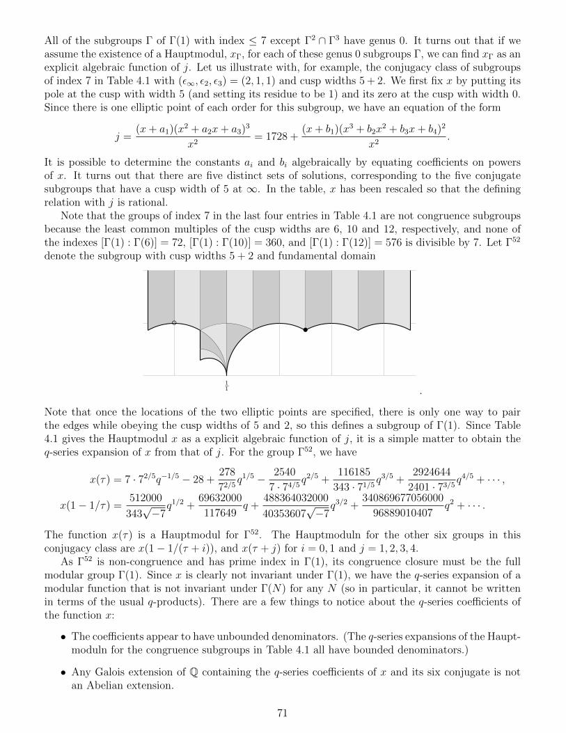
All of the subgroups Γ of Γ(1) with index ≤ 7 except Γ2 ∩ Γ3 have genus 0. It turns out that if weassume the existence of a Hauptmodul, xΓ, for each of these genus 0 subgroups Γ, we can find xΓ as anexplicit algebraic function of j. Let us illustrate with, for example, the conjugacy class of subgroupsof index 7 in Table 4.1 with (ε∞, ε2, ε3) = (2, 1, 1) and cusp widths 5 + 2. We first fix x by putting itspole at the cusp with width 5 (and setting its residue to be 1) and its zero at the cusp with width 0.Since there is one elliptic point of each order for this subgroup, we have an equation of the form
j =(x+ a1)(x2 + a2x+ a3)3
x2= 1728 +
(x+ b1)(x3 + b2x2 + b3x+ b4)2
x2.
It is possible to determine the constants ai and bi algebraically by equating coefficients on powersof x. It turns out that there are five distinct sets of solutions, corresponding to the five conjugatesubgroups that have a cusp width of 5 at ∞. In the table, x has been rescaled so that the definingrelation with j is rational.
Note that the groups of index 7 in the last four entries in Table 4.1 are not congruence subgroupsbecause the least common multiples of the cusp widths are 6, 10 and 12, respectively, and none ofthe indexes [Γ(1) : Γ(6)] = 72, [Γ(1) : Γ(10)] = 360, and [Γ(1) : Γ(12)] = 576 is divisible by 7. Let Γ52
denote the subgroup with cusp widths 5 + 2 and fundamental domain
11
•
.
Note that once the locations of the two elliptic points are specified, there is only one way to pairthe edges while obeying the cusp widths of 5 and 2, so this defines a subgroup of Γ(1). Since Table4.1 gives the Hauptmodul x as a explicit algebraic function of j, it is a simple matter to obtain theq-series expansion of x from that of j. For the group Γ52, we have
x(τ) = 7 · 72/5q−1/5 − 28 +278
72/5q1/5 − 2540
7 · 74/5q2/5 +
116185
343 · 71/5q3/5 +
2924644
2401 · 73/5q4/5 + · · · ,
x(1− 1/τ) =512000
343√−7
q1/2 +69632000
117649q +
488364032000
40353607√−7
q3/2 +340869677056000
96889010407q2 + · · · .
The function x(τ) is a Hauptmodul for Γ52. The Hauptmoduln for the other six groups in thisconjugacy class are x(1− 1/(τ + i)), and x(τ + j) for i = 0, 1 and j = 1, 2, 3, 4.
As Γ52 is non-congruence and has prime index in Γ(1), its congruence closure must be the fullmodular group Γ(1). Since x is clearly not invariant under Γ(1), we have the q-series expansion of amodular function that is not invariant under Γ(N) for any N (so in particular, it cannot be writtenin terms of the usual q-products). There are a few things to notice about the q-series coefficients ofthe function x:
• The coefficients appear to have unbounded denominators. (The q-series expansions of the Haupt-moduln for the congruence subgroups in Table 4.1 all have bounded denominators.)
• Any Galois extension of Q containing the q-series coefficients of x and its six conjugate is notan Abelian extension.
71
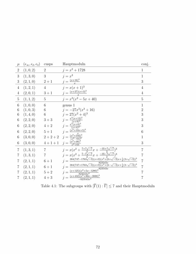
µ (ε∞, ε2, ε3) cusps Hauptmoduln conj.
2 (1, 0, 2) 2 j = x2 + 1728 1
3 (1, 3, 0) 3 j = x3 1
3 (2, 1, 0) 2 + 1 j = (x+16)3
x3
4 (1, 2, 1) 4 j = x(x+ 1)3 4
4 (2, 0, 1) 3 + 1 j = (x+27)(x+3)3
x4
5 (1, 1, 2) 5 j = x3(x2 − 5x+ 40) 5
6 (1, 0, 0) 6 genus 1 16 (1, 0, 3) 6 j = −27x3(x3 + 16) 26 (1, 4, 0) 6 j = 27(x2 + 4)3 3
6 (2, 2, 0) 3 + 3 j = x3(x+12)3
(x+9)3 3
6 (2, 2, 0) 4 + 2 j = x3(x+8)3
(x+4)2 3
6 (2, 2, 0) 5 + 1 j = (x2+10x+5)3
x6
6 (3, 0, 0) 2 + 2 + 2 j = (x2+192)3
(x2−64)2 1
6 (3, 0, 0) 4 + 1 + 1 j = (x2+48)3
x2+643
7 (1, 3, 1) 7 j = x(x2 + 7+7√−7
2x+ −35+7
√−7
2)3 7
7 (1, 3, 1) 7 j = x(x2 + 7−7√−7
2x+ −35−7
√−7
2)3 7
7 (2, 1, 1) 6 + 1 j =384(747−1763
√−3)(x+9)(x2+(6+
√−3)x+ 1
2(3+√−3))3
823543x7
7 (2, 1, 1) 6 + 1 j =384(747+1763
√−3)(x+9)(x2+(6−
√−3)x+ 1
2(3−√−3))3
823543x7
7 (2, 1, 1) 5 + 2 j = (x+125)(x2+5x−1280)3
823543x2 7
7 (2, 1, 1) 4 + 3 j = (x+432)(x2+80x−3888)3
−823543x3 7
Table 4.1: The subgroups with [Γ(1) : Γ] ≤ 7 and their Hauptmoduln
72
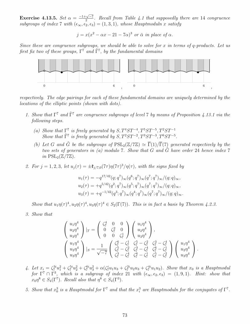
Exercise 4.13.5. Set α = −1+√−7
2. Recall from Table 4.1 that supposedly there are 14 congruence
subgroups of index 7 with (ε∞, ε2, ε3) = (1, 3, 1), whose Hauptmoduln x satisfy
j = x(x2 − αx− 21− 7α)3 or α in place of α.
Since these are congruence subgroups, we should be able to solve for x in terms of q-products. Let usfirst fix two of these groups, Γ7 and Γ7, by the fundamental domains
0 6
•
, 0 6
•
,
respectively. The edge pairings for each of these fundamental domains are uniquely determined by thelocations of the elliptic points (shown with dots).
1. Show that Γ7 and Γ7 are congruence subgroups of level 7 by means of Proposition 4.13.1 via thefollowing steps.
(a) Show that Γ7 is freely generated by S, T 4ST−4, T 5ST−5, T 2ST−1
Show that Γ7 is freely generated by S, T 2ST−2, T 3ST−3, T 6ST−5.
(b) Let G and G be the subgroups of PSL2(Z/7Z) ' Γ(1)/Γ(7) generated respectively by thetwo sets of generators in (a) modulo 7. Show that G and G have order 24 hence index 7in PSL2(Z/7Z).
2. For j = 1, 2, 3, let uj(τ) = ±kj/7,0(7τ)η(7τ)3/η(τ), with the signs fixed by
u1(τ) = −q17/42(q; q7)∞(q6; q7)∞(q7; q7)∞/(q; q)∞,
u2(τ) = +q5/42(q2; q7)∞(q5; q7)∞(q7; q7)∞/(q; q)∞,
u3(τ) = +q−1/42(q3; q7)∞(q4; q7)∞(q7; q7)∞/(q; q)∞.
Show that u1η(τ)4, u2η(τ)4, u3η(τ)4 ∈ S2(Γ(7)). This is in fact a basis by Theorem 4.2.3.
3. Show that u1η4
u2η4
u3η4
|T =
ζ47 0 00 ζ2
7 00 0 ζ1
7
u1η4
u2η4
u3η4
,
u1η4
u2η4
u3η4
|S =1√−7
ζ67 − ζ1
7 ζ57 − ζ2
7 ζ37 − ζ4
7
ζ57 − ζ2
7 ζ37 − ζ4
7 ζ67 − ζ1
7
ζ37 − ζ4
7 ζ67 − ζ1
7 ζ57 − ζ2
7
u1η4
u2η4
u3η4
.
4. Let xi = ζ3i7 u
21 + ζ5i
7 u22 + ζ6i
7 u23 + α(ζ i7u1u3 + ζ2i
7 u2u3 + ζ4i7 u1u2). Show that x0 is a Hauptmodul
for Γ7 ∩ Γ3, which is a subgroup of index 21 with (ε∞, ε2, ε3) = (1, 9, 1). Hint: show thatx0η
8 ∈ S4(Γ7). Recall also that η8 ∈ S4(Γ3).
5. Show that x30 is a Hauptmodul for Γ7 and that the x3
i are Hauptmoduln for the conjugates of Γ7.
73
Chapter 5
Hecke Operators
5.1 Definition of the Hecke operators
5.2 Eigenforms
5.3 Newforms
74
Chapter 6
Modular Forms mod p
6.1 The structure of modular forms on SL2(Z) mod p
6.2 The congruences for p(n) mod 5,7,11 are the Unique Ra-
manujan Congruences
6.3 24n ≡ 1 mod 5a7b11c implies p(n) ≡ 0 mod 5a7bb2c+111c
75
Chapter 7
Modular Equations and Singular Values
7.1 Modular equations for j
Proposition 7.1.1 (Classical modular equation). For any integer n ≥ 2 there is a polynomialΦn(X, Y ) of degree φ(n) = n
∏p|n(1 + 1/p) in X and Y such that:
1. Φn(X, Y ) is irreducible.
2. Φn(X, Y ) is symmetric in X and Y .
3. Φn(X,X) has leading coefficient ±1 if n is not a square.
4. The zeros of Φn(X, j(τ)) occur exactly at the points
X = j
(ατ + β
δ
),
αδ = n0 ≤ β < δgcd(α, β, δ) = 1
.
Proof. This polynomial can be given as
Φn(X, Y ) =∏ad=n
0≤b<d(a,b,d)=1
(X − j
(aτ + b
d
)), (7.1.1)
where the coefficients of Xk on the right hand side should expressed as polynomials in Y for Y = j(τ)....
Proposition 7.1.2 (Canonical modular equation). For any integer n ≥ 2 there is an irreduciblepolynomial Ψn(X, Y ) of degree ψ(n) in X and Y such that Φn(fn(τ), j(τ)) = 0, where
fn(τ) =
(η(nτ)
η(τ)
) 24(24,n−1)
.
76
7.2 Modular equations for the Weber functions
Weber’s functions are defined as
γ3(τ) =√j(τ)− 1728 =
E6(τ)
η(τ)12
γ2(τ) = (j(τ))1/3 =E4(τ)
η(τ)8
f(τ) = ζ−148
η(τ+1
2
)η(τ)
f1(τ) =η(τ2
)η(τ)
f2(τ) =η (2τ)
η(τ)
Proposition 7.2.1.
γ3(τ) ∈M !0(Γ(2)),
γ2(τ) ∈M !0(Γ(3)),
f(τ)24, f1(τ)24, f2(τ)24 ∈M !0(Γ(2)),
f(τ)3, f1(τ)3, f2(τ)3 ∈M !0(Γ(16)),
f(τ), f1(τ), f2(τ) ∈M !0(Γ(48)).
7.3 Quadratic Forms
Let n < 0 be an square free integer and consider the field K = Q(√n)). The ring of integers in K
can be given as
OK =
Z + Z
√n , n 6≡ 1 mod 4
Z + Z−1+√n
2, n ≡ 1 mod 4
.
Therefore, the discriminant of K is given as
disc(K) =
4n , n 6≡ 1 mod 4
n , n ≡ 1 mod 4. (7.3.1)
Definition 7.3.1.
1. A negative integer d is called a discriminant if d ≡ 0, 1 mod 4.
2. A negative integer ∆ is called a fundamental discriminant if it can be obtained from some squarefree n by formula (7.3.1). These are the numbers ∆ such that
∆ ≡ 1 mod 4 and ∆ is square free
or ∆ ≡ 8, 12 mod 16 and ∆/4 is square free.
3. Any discriminant d can be written uniquely as d = f 2∆ where ∆ is a fundamental discriminantand f > 0 is an integer. This f is called the conductor of the discriminant d.
77
Definition 7.3.2. Associate with triple of integers (a, b, c) such that a > 0,b2− 4ac < 0 the followingobjects
1. the positive definite quadratic form ax2 + bxy + cy2
2. the discriminant b2 − 4ac
3. τa,b,c = −b+√d
2a∈ H
4. the following operation of Z2×2 on quadratics forms
M ∈ Z2×2 : ax2 + bxy + cy2 7→ aX2 + bXY + cY 2 with
(XY
)= M
(xy
).
Definition 7.3.3.
1. A quadratic form (a, b, c) is called reduced if
0 ≤ |b| ≤ a ≤ c and b ≥ 0 whenever a = |b| or a = c.
2. A quadratic form (a, b, c) is called primitive if gcd(a, b, c) = 1.
Proposition 7.3.4. Every quadratic form is equivalent (under Γ(1)) to a reduced form, and no twodistinct reduced forms are equivalent.
Proof. The condition for (a, b, c) reduced is exactly
|Re(τ)| ≤ 1
2and |τ | ≥ 1 and Re(τ) ≤ 0 whenever |Re(τ)| = 1
2or |τ | = 1.
for τ = −b+√d
2a. This is exactly the fundamental domain for Γ(1).
Definition 7.3.5. Let H(d) denote the equivalent classes of primitive forms of a given discriminantd under the action of Γ(1). Also let h(d) denote the size of H(d).
Proposition 7.3.6. h(d) <∞.
Proof. If (a, b, c) is a reduced form with discriminant d then we see b2 ≤ ac ≤ −d/3. There can onlybe a finite number of forms satisfying this.
Example 7.3.7.
h(−163) = 1 H(−163) = (1, 1, 41)h(−160) = 4 H(−160) = (1, 0, 40), (5, 0, 8), (4, 4, 11), (7, 6, 7)
7.4 Singular Values of the j Function
Proposition 7.4.1. For any discriminant d, the polynomial
Hjd(X) =
∏(a,b,c)∈H(d)
(X − j
(−b+√d
2a
))has integer coefficients. Furthermore, if d = r2− 4n for any integers r and n with n > 1, then Hj
d(X)divides Φn(X,X) (the modular equation for j).
Remark 7.4.2. It seems that the full force of class field theory is required to show that Hjd(X) is
irreducible and the Galois group over Q(√−d) is isomorphic to the class group, but we will not need
this fact for our purposes.
78
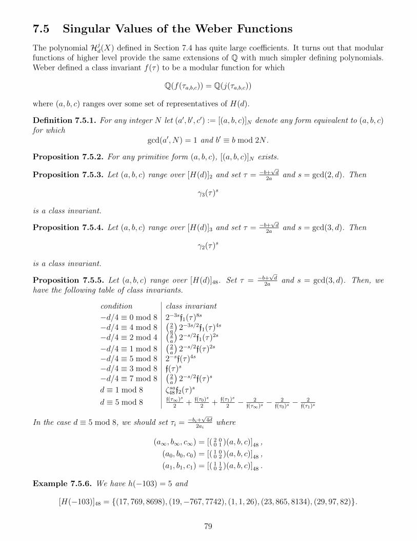
7.5 Singular Values of the Weber Functions
The polynomial Hjd(X) defined in Section 7.4 has quite large coefficients. It turns out that modular
functions of higher level provide the same extensions of Q with much simpler defining polynomials.Weber defined a class invariant f(τ) to be a modular function for which
Q(f(τa,b,c)) = Q(j(τa,b,c))
where (a, b, c) ranges over some set of representatives of H(d).
Definition 7.5.1. For any integer N let (a′, b′, c′) := [(a, b, c)]N denote any form equivalent to (a, b, c)for which
gcd(a′, N) = 1 and b′ ≡ b mod 2N .
Proposition 7.5.2. For any primitive form (a, b, c), [(a, b, c)]N exists.
Proposition 7.5.3. Let (a, b, c) range over [H(d)]2 and set τ = −b+√d
2aand s = gcd(2, d). Then
γ3(τ)s
is a class invariant.
Proposition 7.5.4. Let (a, b, c) range over [H(d)]3 and set τ = −b+√d
2aand s = gcd(3, d). Then
γ2(τ)s
is a class invariant.
Proposition 7.5.5. Let (a, b, c) range over [H(d)]48. Set τ = −b+√d
2aand s = gcd(3, d). Then, we
have the following table of class invariants.
condition class invariant
−d/4 ≡ 0 mod 8 2−3sf1(τ)8s
−d/4 ≡ 4 mod 8(
2a
)2−3s/2f1(τ)4s
−d/4 ≡ 2 mod 4(
2a
)2−s/2f1(τ)2s
−d/4 ≡ 1 mod 8(
2a
)2−s/2f(τ)2s
−d/4 ≡ 5 mod 8 2−sf(τ)4s
−d/4 ≡ 3 mod 8 f(τ)s
−d/4 ≡ 7 mod 8(
2a
)2−s/2f(τ)s
d ≡ 1 mod 8 ζsa48 f2(τ)s
d ≡ 5 mod 8 f(τ∞)s
2+ f(τ0)s
2+ f(τ1)s
2− 2
f(τ∞)s− 2
f(τ0)s− 2
f(τ1)s
In the case d ≡ 5 mod 8, we should set τi = −bi+√
4d2ai
where
(a∞, b∞, c∞) = [( 2 00 1 )(a, b, c)]48 ,
(a0, b0, c0) = [( 1 00 2 )(a, b, c)]48 ,
(a1, b1, c1) = [( 1 10 2 )(a, b, c)]48 .
Example 7.5.6. We have h(−103) = 5 and
[H(−103)]48 = (17, 769, 8698), (19,−767, 7742), (1, 1, 26), (23, 865, 8134), (29, 97, 82).
79
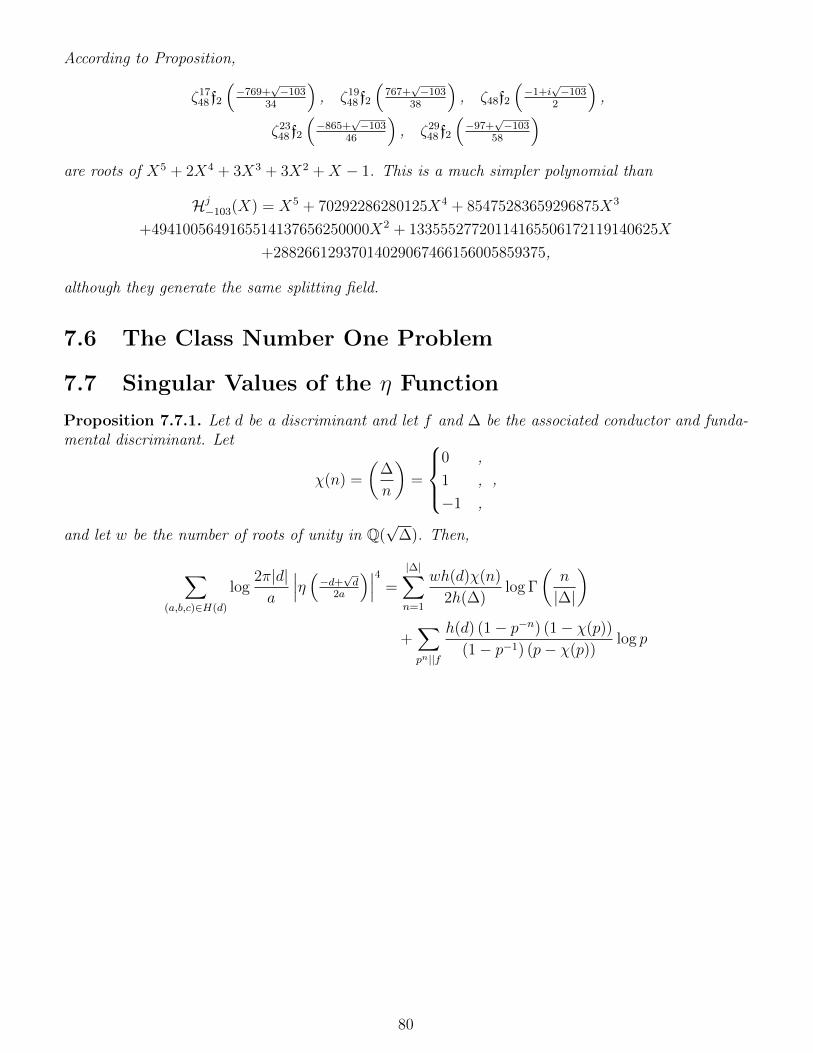
According to Proposition,
ζ1748 f2
(−769+
√−103
34
), ζ19
48 f2
(767+
√−103
38
), ζ48f2
(−1+i
√−103
2
),
ζ2348 f2
(−865+
√−103
46
), ζ29
48 f2
(−97+
√−103
58
)are roots of X5 + 2X4 + 3X3 + 3X2 +X − 1. This is a much simpler polynomial than
Hj−103(X) = X5 + 70292286280125X4 + 85475283659296875X3
+4941005649165514137656250000X2 + 13355527720114165506172119140625X
+28826612937014029067466156005859375,
although they generate the same splitting field.
7.6 The Class Number One Problem
7.7 Singular Values of the η Function
Proposition 7.7.1. Let d be a discriminant and let f and ∆ be the associated conductor and funda-mental discriminant. Let
χ(n) =
(∆
n
)=
0 ,
1 ,
−1 ,
,
and let w be the number of roots of unity in Q(√
∆). Then,
∑(a,b,c)∈H(d)
log2π|d|a
∣∣∣η (−d+√d
2a
)∣∣∣4 =
|∆|∑n=1
wh(d)χ(n)
2h(∆)log Γ
(n
|∆|
)
+∑pn||f
h(d) (1− p−n) (1− χ(p))
(1− p−1) (p− χ(p))log p
80
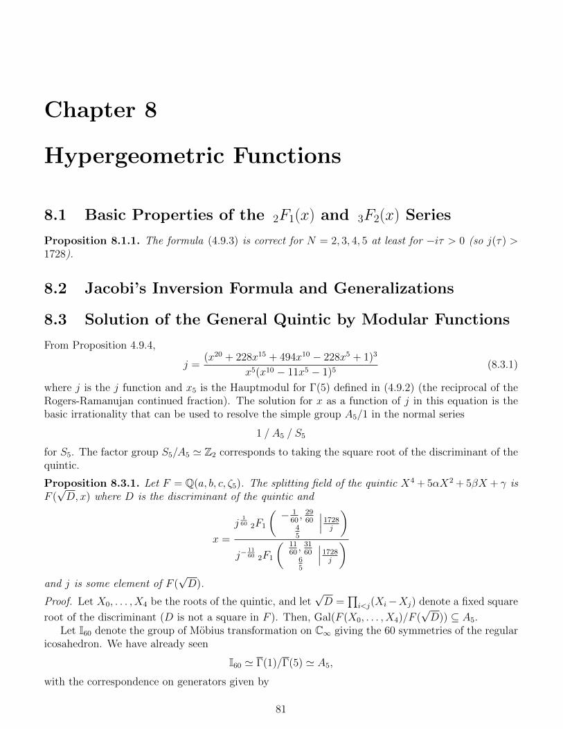
Chapter 8
Hypergeometric Functions
8.1 Basic Properties of the 2F1(x) and 3F2(x) Series
Proposition 8.1.1. The formula (4.9.3) is correct for N = 2, 3, 4, 5 at least for −iτ > 0 (so j(τ) >1728).
8.2 Jacobi’s Inversion Formula and Generalizations
8.3 Solution of the General Quintic by Modular Functions
From Proposition 4.9.4,
j =(x20 + 228x15 + 494x10 − 228x5 + 1)3
x5(x10 − 11x5 − 1)5(8.3.1)
where j is the j function and x5 is the Hauptmodul for Γ(5) defined in (4.9.2) (the reciprocal of theRogers-Ramanujan continued fraction). The solution for x as a function of j in this equation is thebasic irrationality that can be used to resolve the simple group A5/1 in the normal series
1 / A5 / S5
for S5. The factor group S5/A5 ' Z2 corresponds to taking the square root of the discriminant of thequintic.
Proposition 8.3.1. Let F = Q(a, b, c, ζ5). The splitting field of the quintic X4 + 5αX2 + 5βX + γ isF (√D, x) where D is the discriminant of the quintic and
x =
j160 2F1
(− 1
60, 29
6045
∣∣∣1728j
)j−
1160 2F1
( 1160, 31
6065
∣∣∣1728j
)and j is some element of F (
√D).
Proof. Let X0, . . . , X4 be the roots of the quintic, and let√D =
∏i<j(Xi−Xj) denote a fixed square
root of the discriminant (D is not a square in F ). Then, Gal(F (X0, . . . , X4)/F (√D)) ⊆ A5.
Let I60 denote the group of Mobius transformation on C∞ giving the 60 symmetries of the regularicosahedron. We have already seen
I60 ' Γ(1)/Γ(5) ' A5,
with the correspondence on generators given by
81
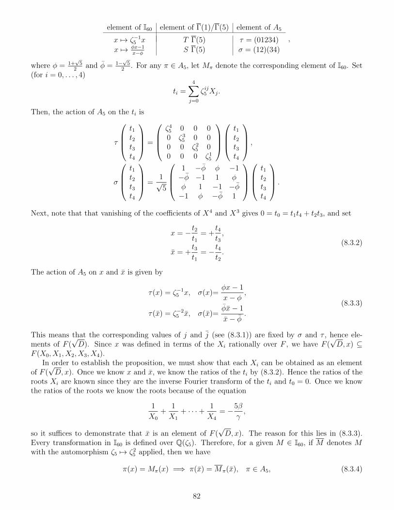
element of I60 element of Γ(1)/Γ(5) element of A5
x 7→ ζ−15 x T Γ(5) τ = (01234)
x 7→ φx−1x−φ S Γ(5) σ = (12)(34)
,
where φ = 1+√
52
and φ = 1−√
52
. For any π ∈ A5, let Mπ denote the corresponding element of I60. Set(for i = 0, . . . , 4)
ti =4∑j=0
ζ ij5 Xj.
Then, the action of A5 on the ti is
τ
t1t2t3t4
=
ζ4
5 0 0 00 ζ3
5 0 00 0 ζ2
5 00 0 0 ζ1
5
t1t2t3t4
,
σ
t1t2t3t4
=1√5
1 −φ φ −1−φ −1 1 φφ 1 −1 −φ−1 φ −φ 1
t1t2t3t4
.
Next, note that that vanishing of the coefficients of X4 and X3 gives 0 = t0 = t1t4 + t2t3, and set
x = −t2t1
= +t4t3
,
x = +t3t1
= −t4t2
.(8.3.2)
The action of A5 on x and x is given by
τ(x) = ζ−15 x, σ(x)=
φx− 1
x− φ,
τ(x) = ζ−25 x, σ(x)=
φx− 1
x− φ.
(8.3.3)
This means that the corresponding values of j and j (see (8.3.1)) are fixed by σ and τ , hence ele-ments of F (
√D). Since x was defined in terms of the Xi rationally over F , we have F (
√D, x) ⊆
F (X0, X1, X2, X3, X4).In order to establish the proposition, we must show that each Xi can be obtained as an element
of F (√D, x). Once we know x and x, we know the ratios of the ti by (8.3.2). Hence the ratios of the
roots Xi are known since they are the inverse Fourier transform of the ti and t0 = 0. Once we knowthe ratios of the roots we know the roots because of the equation
1
X0
+1
X1
+ · · ·+ 1
X4
= −5β
γ,
so it suffices to demonstrate that x is an element of F (√D, x). The reason for this lies in (8.3.3).
Every transformation in I60 is defined over Q(ζ5). Therefore, for a given M ∈ I60, if M denotes Mwith the automorphism ζ5 7→ ζ2
5 applied, then we have
π(x) = Mπ(x) =⇒ π(x) = Mπ(x), π ∈ A5, (8.3.4)
82
since this holds on generators. Now let M1, · · · ,M60 denote the elements of I60 so that Mi(x)i isa list of conjugates of x under A5. Since (8.3.1) has disinct roots as long as j 6= 0, 1728,∞, thislist contains 60 distinct elements. From (8.3.4) we see that Mi(x)i and M i(x)i are permutedidentically under A5, that is
π(Mi(x)) = Mj(x) =⇒ π(M i(x)) = M j(x), π ∈ A5.
This means that the solutions for the ak in the linear system
M i(x) =60∑k=1
akMi(x)k−1, i = 1, . . . , 60
are all fixed by A5 hence elements of F (√D).
Remark 8.3.2. It is possible to be much more explicit about the relationship between x and x. Infact, we have
√x11 − 11x6 − x√
j − 1728
(7x5 − 1)x+ x7 + 7x2
(x13 + 39x8 − 26x3)x− 26x10 − 39x5 + 1∈ F (
√D).
See [5].
83
Chapter 9
Mock Modular Forms
84
Bibliography
[1] T. M. Apostol, Modular Functions and Dirichlet Series in Number Theory, 2nd ed., New York:Springer-Verlag, 1997.
[2] A. O. L. Atkin, J. N. O’Brien, Some properties of p(n) and c(n) modulo powers of 13. Trans.Amer. Math. Soc. 126 (1976), 442-459.
[3] Borwein, J. M. and Borwein, P. B., A cubic counterpart of Jacobis identity and the AGM, Trans.Amer. Math. Soc. 323 (1991), 691-701.
[4] F. Diamond, J. Shurman, A First Course in Modular Forms, New York: Springer-Verlag, 2005.
[5] P. Gordon. Ueber die Auflosung der Gleichungen vom funften Grade. Math. Ann., 13:375404,1869.
[6] T. Horie, N. Kanou, Certain Modular Functions Similar to the Dedekind eta Function, Abh.Math. Sem. Univ. Hamburg 72 (2002), 89-117.
[7] N. Ishida, Generators and equations for modular function fields of principal congruence sub-groups, Acta Arithmetica LXXXV.3 (1998)
[8] M. I. Knopp, Modular Function in Analytic Number Theory, 2nd ed., Chelsea, New York, 1993.
[9] R. S. Kulkarni, An arithmetic geometric method in the study of the subgroups of the modulargroup, American Journal of Mathematics 113 (1991), no. 6, 1053–1133.
[10] C. A. Kurth, L. Long, Computations with Finite Index Subgroups of PSL2(Z) using Farey Sym-bols.
[11] A. Lubotzky, Counting Finite Index Subgroups.
[12] M. Newman, Asymptotic formulas related to free products of cyclic groups, Math. Comp. 30(1976), 838–846
[13] M. Newman, Classification of normal subgroups of the modular group.
[14] S. A. Vidal, Sur le classification et le denombrement des sous-groupes du groupemodulaire et de leurs classes de conjugaison. Pub. IRMA, Lille 66(II):1-35, 2006.Preprint:http://arxiv.org/abs/math.CO/0702223
[15] D. Goldfeld, A. Lubotzky, L. Pyber, Counting Congruence Subgroups, Acta Mathematica, 2004,Volume 193, Issue 1, pp 73-104
[16] T. Hsu, IDENTIFYING CONGRUENCE SUBGROUPS OF THE MODULAR GROUP. Proc.Amer. Math. Soc. (124), no. 5, May 1996
85