curnow SI revised proofs - pnas.org · ! 3!! Figure, S3:!Relationship! between! equilibrium and!...

1

SUPPLEMENTARY INFORMATION FOR CURNOW ET AL

Figure S1: Equilibrium unfolding curves for alanine mutants in bR helix G. Raw data, with Y-axis showing chromophore absorbance at 560 nm.

2

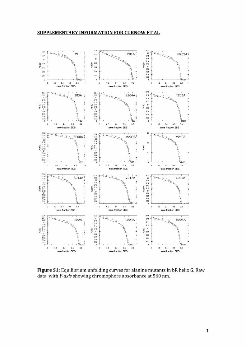
Figure S2: Kinetic chevron plots for systematic mutations through helix G (a-‐k)

and mutations introduced for double-‐mutant cycles (l-‐r). L201A (a) is a

stabilizing mutation and all the others are destabilizing. V210A (h), V217A (i),

L223A (k), D96A (l), S226A (n), S193A/E204A (p), D212A (q) and Y185F/D212A

(r) showed substantial changes in kfH2O and mkf.

3

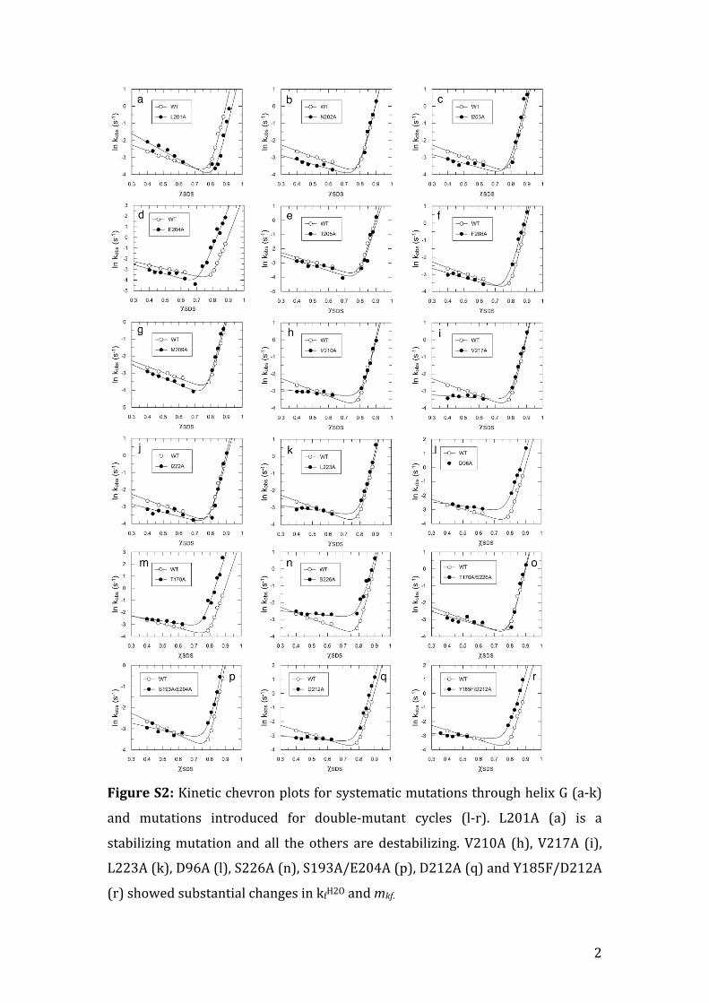
Figure S3: Relationship between equilibrium and kinetic measurements of

ΔΔGuH2O for Ala mutations in helix G.

4

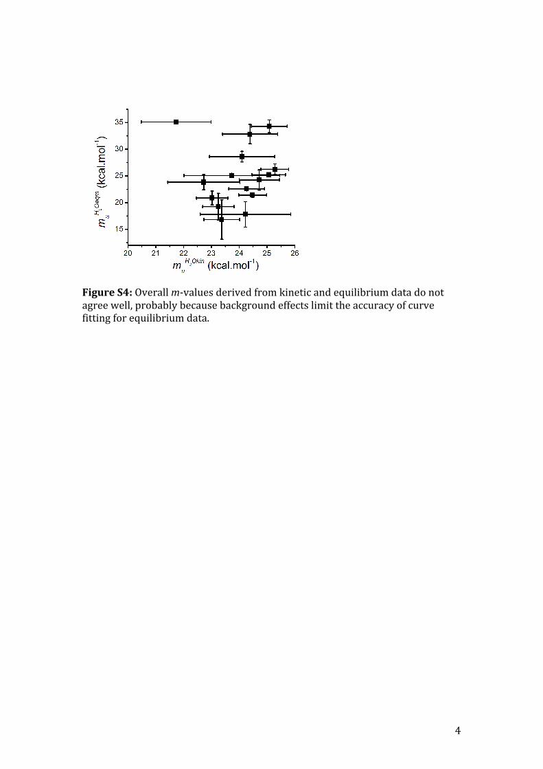
Figure S4: Overall m-‐values derived from kinetic and equilibrium data do not agree well, probably because background effects limit the accuracy of curve fitting for equilibrium data.

5

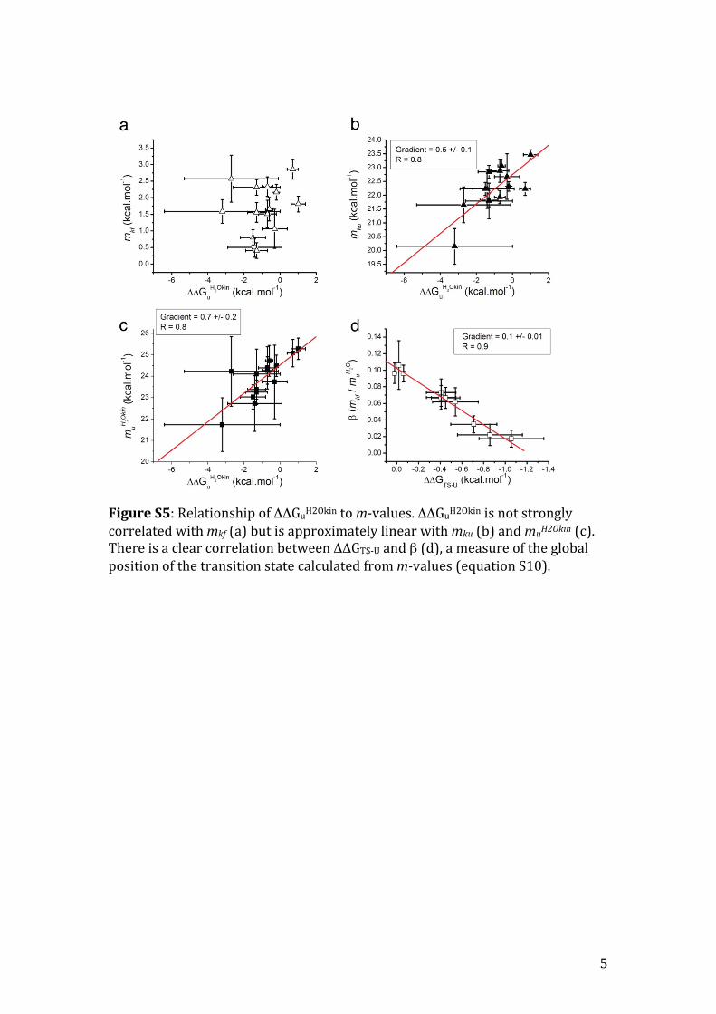
Figure S5: Relationship of ΔΔGuH2Okin to m-‐values. ΔΔGuH2Okin is not strongly correlated with mkf (a) but is approximately linear with mku (b) and muH2Okin (c). There is a clear correlation between ΔΔGTS-‐U and β (d), a measure of the global position of the transition state calculated from m-values (equation S10).

6

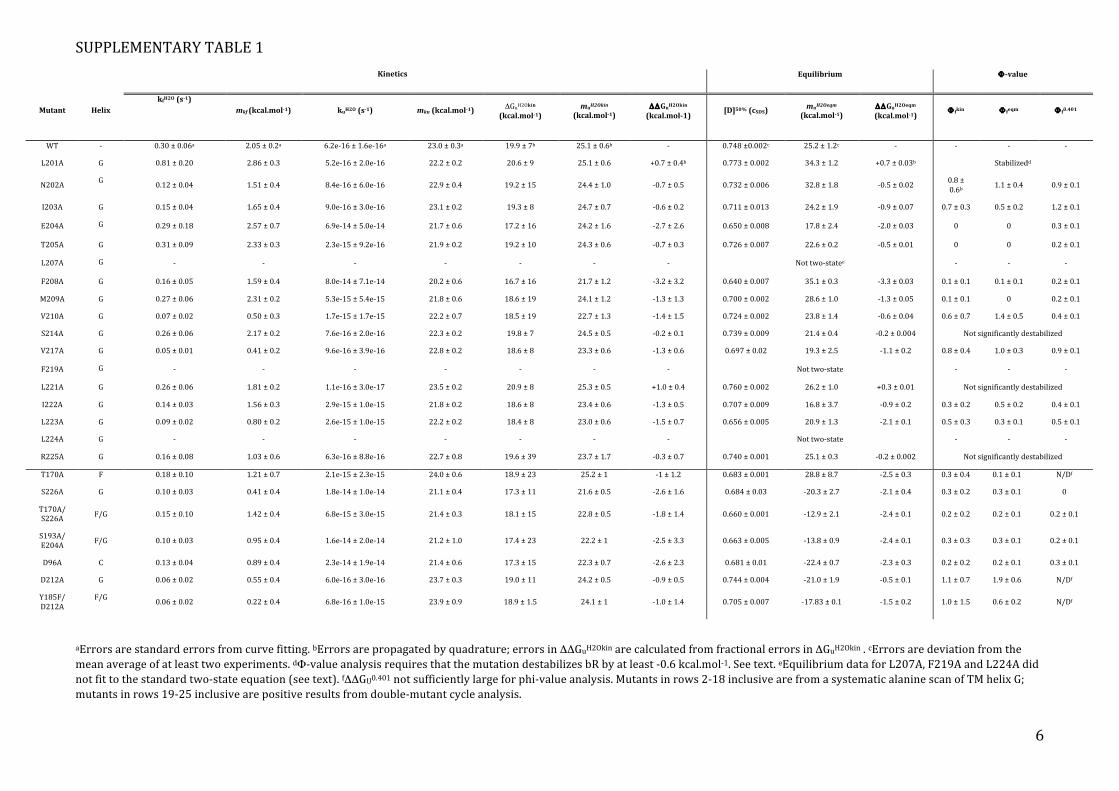
SUPPLEMENTARY TABLE 1

Kinetics Equilibrium Φ-value

Mutant Helix kfH2O (s-1)

mkf (kcal.mol-1) kuH2O (s-1) mku (kcal.mol-1)

ΔGuH2Okin (kcal.mol-1)

muH2Okin (kcal.mol-1)

ΔΔGuH2Okin (kcal.mol-1)

[D]50% (cSDS) muH2Oeqm

(kcal.mol-1) ΔΔGuH2Oeqm (kcal.mol-1)

Φ fkin Φ feqm Φ f0.401

WT -‐ 0.30 ± 0.06a 2.05 ± 0.2a 6.2e-‐16 ± 1.6e-‐16a 23.0 ± 0.3a 19.9 ± 7b 25.1 ± 0.6b -‐ 0.748 ±0.002c 25.2 ± 1.2c -‐ -‐ -‐ -‐

L201A G 0.81 ± 0.20 2.86 ± 0.3 5.2e-‐16 ± 2.0e-‐16 22.2 ± 0.2 20.6 ± 9 25.1 ± 0.6 +0.7 ± 0.4b 0.773 ± 0.002 34.3 ± 1.2 +0.7 ± 0.03b Stabilizedd

N202A G 0.12 ± 0.04 1.51 ± 0.4 8.4e-‐16 ± 6.0e-‐16 22.9 ± 0.4 19.2 ± 15 24.4 ± 1.0 -‐0.7 ± 0.5 0.732 ± 0.006 32.8 ± 1.8 -‐0.5 ± 0.02 0.8 ± 0.6b 1.1 ± 0.4 0.9 ± 0.1

I203A G 0.15 ± 0.04 1.65 ± 0.4 9.0e-‐16 ± 3.0e-‐16 23.1 ± 0.2 19.3 ± 8 24.7 ± 0.7 -‐0.6 ± 0.2 0.711 ± 0.013 24.2 ± 1.9 -‐0.9 ± 0.07 0.7 ± 0.3 0.5 ± 0.2 1.2 ± 0.1

E204A G 0.29 ± 0.18 2.57 ± 0.7 6.9e-‐14 ± 5.0e-‐14 21.7 ± 0.6 17.2 ± 16 24.2 ± 1.6 -‐2.7 ± 2.6 0.650 ± 0.008 17.8 ± 2.4 -‐2.0 ± 0.03 0 0 0.3 ± 0.1

T205A G 0.31 ± 0.09 2.33 ± 0.3 2.3e-‐15 ± 9.2e-‐16 21.9 ± 0.2 19.2 ± 10 24.3 ± 0.6 -‐0.7 ± 0.3 0.726 ± 0.007 22.6 ± 0.2 -‐0.5 ± 0.01 0 0 0.2 ± 0.1

L207A G -‐ -‐ -‐ -‐ -‐ -‐ -‐ Not two-‐statee -‐ -‐ -‐

F208A G 0.16 ± 0.05 1.59 ± 0.4 8.0e-‐14 ± 7.1e-‐14 20.2 ± 0.6 16.7 ± 16 21.7 ± 1.2 -‐3.2 ± 3.2 0.640 ± 0.007 35.1 ± 0.3 -‐3.3 ± 0.03 0.1 ± 0.1 0.1 ± 0.1 0.2 ± 0.1

M209A G 0.27 ± 0.06 2.31 ± 0.2 5.3e-‐15 ± 5.4e-‐15 21.8 ± 0.6 18.6 ± 19 24.1 ± 1.2 -‐1.3 ± 1.3 0.700 ± 0.002 28.6 ± 1.0 -‐1.3 ± 0.05 0.1 ± 0.1 0 0.2 ± 0.1

V210A G 0.07 ± 0.02 0.50 ± 0.3 1.7e-‐15 ± 1.7e-‐15 22.2 ± 0.7 18.5 ± 19 22.7 ± 1.3 -‐1.4 ± 1.5 0.724 ± 0.002 23.8 ± 1.4 -‐0.6 ± 0.04 0.6 ± 0.7 1.4 ± 0.5 0.4 ± 0.1

S214A G 0.26 ± 0.06 2.17 ± 0.2 7.6e-‐16 ± 2.0e-‐16 22.3 ± 0.2 19.8 ± 7 24.5 ± 0.5 -‐0.2 ± 0.1 0.739 ± 0.009 21.4 ± 0.4 -‐0.2 ± 0.004 Not significantly destabilized

V217A G 0.05 ± 0.01 0.41 ± 0.2 9.6e-‐16 ± 3.9e-‐16 22.8 ± 0.2 18.6 ± 8 23.3 ± 0.6 -‐1.3 ± 0.6 0.697 ± 0.02 19.3 ± 2.5 -‐1.1 ± 0.2 0.8 ± 0.4 1.0 ± 0.3 0.9 ± 0.1

F219A G -‐ -‐ -‐ -‐ -‐ -‐ -‐ Not two-‐state -‐ -‐ -‐

L221A G 0.26 ± 0.06 1.81 ± 0.2 1.1e-‐16 ± 3.0e-‐17 23.5 ± 0.2 20.9 ± 8 25.3 ± 0.5 +1.0 ± 0.4 0.760 ± 0.002 26.2 ± 1.0 +0.3 ± 0.01 Not significantly destabilized

I222A G 0.14 ± 0.03 1.56 ± 0.3 2.9e-‐15 ± 1.0e-‐15 21.8 ± 0.2 18.6 ± 8 23.4 ± 0.6 -‐1.3 ± 0.5 0.707 ± 0.009 16.8 ± 3.7 -‐0.9 ± 0.2 0.3 ± 0.2 0.5 ± 0.2 0.4 ± 0.1

L223A G 0.09 ± 0.02 0.80 ± 0.2 2.6e-‐15 ± 1.0e-‐15 22.2 ± 0.2 18.4 ± 8 23.0 ± 0.6 -‐1.5 ± 0.7 0.656 ± 0.005 20.9 ± 1.3 -‐2.1 ± 0.1 0.5 ± 0.3 0.3 ± 0.1 0.5 ± 0.1

L224A G -‐ -‐ -‐ -‐ -‐ -‐ -‐ Not two-‐state -‐ -‐ -‐

R225A G 0.16 ± 0.08 1.03 ± 0.6 6.3e-‐16 ± 8.8e-‐16 22.7 ± 0.8 19.6 ± 39 23.7 ± 1.7 -‐0.3 ± 0.7 0.740 ± 0.001 25.1 ± 0.3 -‐0.2 ± 0.002 Not significantly destabilized

T170A F 0.18 ± 0.10 1.21 ± 0.7 2.1e-‐15 ± 2.3e-‐15 24.0 ± 0.6 18.9 ± 23 25.2 ± 1 -‐1 ± 1.2 0.683 ± 0.001 28.8 ± 8.7 -‐2.5 ± 0.3 0.3 ± 0.4 0.1 ± 0.1 N/Df

S226A G 0.10 ± 0.03 0.41 ± 0.4 1.8e-‐14 ± 1.0e-‐14 21.1 ± 0.4 17.3 ± 11 21.6 ± 0.5 -‐2.6 ± 1.6 0.684 ± 0.03 -‐20.3 ± 2.7 -‐2.1 ± 0.4 0.3 ± 0.2 0.3 ± 0.1 0

T170A/ S226A F/G 0.15 ± 0.10 1.42 ± 0.4 6.8e-‐15 ± 3.0e-‐15 21.4 ± 0.3 18.1 ± 15 22.8 ± 0.5 -‐1.8 ± 1.4 0.660 ± 0.001 -‐12.9 ± 2.1 -‐2.4 ± 0.1 0.2 ± 0.2 0.2 ± 0.1 0.2 ± 0.1

S193A/ E204A F/G 0.10 ± 0.03 0.95 ± 0.4 1.6e-‐14 ± 2.0e-‐14 21.2 ± 1.0 17.4 ± 23 22.2 ± 1 -‐2.5 ± 3.3 0.663 ± 0.005 -‐13.8 ± 0.9 -‐2.4 ± 0.1 0.3 ± 0.3 0.3 ± 0.1 0.2 ± 0.1

D96A C 0.13 ± 0.04 0.89 ± 0.4 2.3e-‐14 ± 1.9e-‐14 21.4 ± 0.6 17.3 ± 15 22.3 ± 0.7 -‐2.6 ± 2.3 0.681 ± 0.01 -‐22.4 ± 0.7 -‐2.3 ± 0.3 0.2 ± 0.2 0.2 ± 0.1 0.3 ± 0.1

D212A G 0.06 ± 0.02 0.55 ± 0.4 6.0e-‐16 ± 3.0e-‐16 23.7 ± 0.3 19.0 ± 11 24.2 ± 0.5 -‐0.9 ± 0.5 0.744 ± 0.004 -‐21.0 ± 1.9 -‐0.5 ± 0.1 1.1 ± 0.7 1.9 ± 0.6 N/Df

Y185F/ D212A

F/G 0.06 ± 0.02 0.22 ± 0.4 6.8e-‐16 ± 1.0e-‐15 23.9 ± 0.9 18.9 ± 1.5 24.1 ± 1 -‐1.0 ± 1.4 0.705 ± 0.007 -‐17.83 ± 0.1 -‐1.5 ± 0.2 1.0 ± 1.5 0.6 ± 0.2 N/Df

aErrors are standard errors from curve fitting. bErrors are propagated by quadrature; errors in ΔΔGuH2Okin are calculated from fractional errors in ΔGuH2Okin . cErrors are deviation from the mean average of at least two experiments. dΦ-‐value analysis requires that the mutation destabilizes bR by at least -‐0.6 kcal.mol-‐1. See text. eEquilibrium data for L207A, F219A and L224A did not fit to the standard two-‐state equation (see text). fΔΔGU0.401 not sufficiently large for phi-‐value analysis. Mutants in rows 2-‐18 inclusive are from a systematic alanine scan of TM helix G; mutants in rows 19-‐25 inclusive are positive results from double-‐mutant cycle analysis.

7

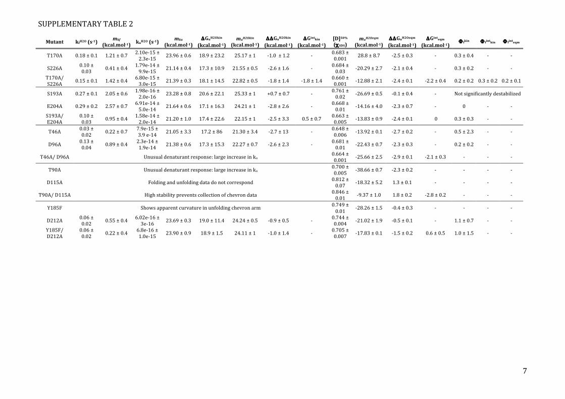
SUPPLEMENTARY TABLE 2

Mutant kfH2O (s-1) mkf

(kcal.mol-1) kuH2O (s-1)

mku (kcal.mol-1)

ΔGuH2Okin (kcal.mol-1)

muH2Okin (kcal.mol-1)

ΔΔGuH2Okin (kcal.mol-1)

ΔGintkin

(kcal.mol-1) [D]50% (χSDS)

muH2Oeqm (kcal.mol-1)

ΔΔGuH2Oeqm (kcal.mol-1)

ΔGinteqm (kcal.mol-1)

Φ fkin Φ fintkin Φ finteqm

T170A 0.18 ± 0.1 1.21 ± 0.7 2.10e-‐15 ± 2.3e-‐15 23.96 ± 0.6 18.9 ± 23.2 25.17 ± 1 -‐1.0 ± 1.2 -‐ 0.683 ±

0.001 28.8 ± 8.7 -‐2.5 ± 0.3 -‐ 0.3 ± 0.4 -‐ -‐

S226A 0.10 ± 0.03 0.41 ± 0.4 1.79e-‐14 ±

9.9e-‐15 21.14 ± 0.4 17.3 ± 10.9 21.55 ± 0.5 -‐2.6 ± 1.6 -‐ 0.684 ± 0.03 -‐20.29 ± 2.7 -‐2.1 ± 0.4 -‐ 0.3 ± 0.2 -‐ -‐

T170A/ S226A 0.15 ± 0.1 1.42 ± 0.4 6.80e-‐15 ±

3.0e-‐15 21.39 ± 0.3 18.1 ± 14.5 22.82 ± 0.5 -‐1.8 ± 1.4 -‐1.8 ± 1.4 0.660 ± 0.001 -‐12.88 ± 2.1 -‐2.4 ± 0.1 -‐2.2 ± 0.4 0.2 ± 0.2 0.3 ± 0.2 0.2 ± 0.1

S193A 0.27 ± 0.1 2.05 ± 0.6 1.98e-‐16 ± 2.0e-‐16 23.28 ± 0.8 20.6 ± 22.1 25.33 ± 1 +0.7 ± 0.7 -‐ 0.761 ±

0.02 -‐26.69 ± 0.5 -‐0.1 ± 0.4 -‐ Not significantly destabilized

E204A 0.29 ± 0.2 2.57 ± 0.7 6.91e-‐14 ± 5.0e-‐14 21.64 ± 0.6 17.1 ± 16.3 24.21 ± 1 -‐2.8 ± 2.6 -‐ 0.668 ±

0.01 -‐14.16 ± 4.0 -‐2.3 ± 0.7 -‐ 0 -‐ -‐

S193A/ E204A

0.10 ± 0.03 0.95 ± 0.4 1.58e-‐14 ±

2.0e-‐14 21.20 ± 1.0 17.4 ± 22.6 22.15 ± 1 -‐2.5 ± 3.3 0.5 ± 0.7 0.663 ± 0.005 -‐13.83 ± 0.9 -‐2.4 ± 0.1 0 0.3 ± 0.3 -‐ -‐

T46A 0.03 ± 0.02 0.22 ± 0.7 7.9e-‐15 ±

3.9 e-‐14 21.05 ± 3.3 17.2 ± 86 21.30 ± 3.4 -‐2.7 ± 13 -‐ 0.648 ± 0.006 -‐13.92 ± 0.1 -‐2.7 ± 0.2 -‐ 0.5 ± 2.3 -‐ -‐

D96A 0.13 ± 0.04 0.89 ± 0.4 2.3e-‐14 ±

1.9e-‐14 21.38 ± 0.6 17.3 ± 15.3 22.27 ± 0.7 -‐2.6 ± 2.3 -‐ 0.681 ± 0.01 -‐22.43 ± 0.7 -‐2.3 ± 0.3 -‐ 0.2 ± 0.2 -‐ -‐

T46A/ D96A Unusual denaturant response: large increase in ku 0.664 ± 0.001 -‐25.66 ± 2.5 -‐2.9 ± 0.1 -‐2.1 ± 0.3 -‐ -‐ -‐

T90A Unusual denaturant response: large increase in ku 0.700 ± 0.005 -‐38.66 ± 0.7 -‐2.3 ± 0.2 -‐ -‐ -‐ -‐

D115A Folding and unfolding data do not correspond 0.812 ± 0.07 -‐18.32 ± 5.2 1.3 ± 0.1 -‐ -‐ -‐ -‐

T90A/ D115A High stability prevents collection of chevron data 0.846 ± 0.01 -‐9.37 ± 1.0 1.8 ± 0.2 -‐2.8 ± 0.2 -‐ -‐ -‐

Y185F Shows apparent curvature in unfolding chevron arm 0.749 ± 0.01 -‐28.26 ± 1.5 -‐0.4 ± 0.3 -‐ -‐ -‐ -‐

D212A 0.06 ± 0.02 0.55 ± 0.4 6.02e-‐16 ±

3e-‐16 23.69 ± 0.3 19.0 ± 11.4 24.24 ± 0.5 -‐0.9 ± 0.5 -‐ 0.744 ± 0.004 -‐21.02 ± 1.9 -‐0.5 ± 0.1 -‐ 1.1 ± 0.7 -‐ -‐

Y185F/ D212A

0.06 ± 0.02 0.22 ± 0.4 6.8e-‐16 ±

1.0e-‐15 23.90 ± 0.9 18.9 ± 1.5 24.11 ± 1 -‐1.0 ± 1.4 -‐ 0.705 ± 0.007 -‐17.83 ± 0.1 -‐1.5 ± 0.2 0.6 ± 0.5 1.0 ± 1.5 -‐ -‐

8

SUPPLEMENTARY METHODS

Molecular biology

Site-‐directed mutations were introduced to recombinant WT bacteriorhodopsin in a plasmid

originally constructed by Krebs and coworkers [1] that can be propagated in strains of both

Escherichia coli and Halobium salinarum. Targeted single Ala mutations were introduced

using the Quikchange method (Stratagene) and the identity of each mutant was confirmed by

sequencing. Each mutant was then transformed into the bR-‐deficient Halobium strain L33

according to the method of Cline and Doolittle [2].

Protein expression and purification

Mutants were prepared in the purple membrane form by standard methods [3] after

constitutive expression from the recombinant plasmid. Briefly, transformed L33 cells were

grown to stationary phase in 1L of high salt media (250 g/L NaCl, 20 g/L MgSO4.2H2O, 3 g/L

Sodium citrate, 2 g/L KCl, 10 g/L Peptone LP0037 (Oxoid)) in the presence of 4 µg/ml of the

selective antibiotic mevinolin before being lysed under low salt conditions. The purple

membrane was then isolated by successive rounds of ultracentrifugation. Typical yields were

2-‐3 mg mutant protein per litre Halobium culture. The identity and purity of each mutant was

confirmed by mass spectrometry [4].

Equilibrium thermodynamics

Equilibrium unfolding curves were constructed as previously described [5-‐7] using a CARY

UV/Vis spectrophotometer (Varian) at 25 °C. bR was diluted to 6 µM in mixed lipid/detergent

micelles of 15 mM 1,2-‐Dimyristoyl-‐sn-‐Glycero-‐3-‐phosphocholine (DMPC) and 16 mM 3-‐[(3-‐

Cholamidopropyl)dimethylammonio]-‐1-‐propanesulfonate (CHAPS) in 10 mM sodium

phosphate buffer, pH 6.0. These conditions give one bR monomer per micelle [8]. Small

aliquots of 20% sodium dodecylsulfate (SDS) were introduced to this sample and SDS-‐induced

changes to the folded state of the protein were assessed by monitoring the chromophore

absorbance band at 560 nm. The characteristic retinal chromophore band is sensitive to

conformational change and disappears outright when bR is unfolded. Unfolding curves

generated from this method exhibit a non-‐linear background signal that can complicate curve-‐

fitting procedures. To obtain free energy values, we adopted a similar approach to that used

recently by Bowie and coworkers [9]and calculated changes in free energies by determining

the midpoint and slope of the major unfolding transition from fitting to equation S1 [10-‐12]:

9

Y = (AF + mF*[D]) + (AU + mU*[D])exp(muH2O*([D]-‐[D]50%)/RT)/ 1+ exp(muH2O*([D]-‐[D]50%)/RT)

[Equation S1]

Where AF and AU are the absorbance of the folded and unfolded state respectively and mF and

mU are the associated gradients; muH2O is the slope of the major unfolding transition; [D] is

denaturant concentration; and [D]50% is the denaturant concentration at which the protein is

50% unfolded.

Differences in m-‐value and [D]50% between native and mutant proteins can be used to

determine the overall energetic peturbation caused by the mutation at equilibrium

(ΔΔGuH2Oeqm) according to equation S2:

ΔΔGuH2Oeqm = 0.5 (muH2Owt + muH2Omut)*Δ[D]50% [Equation S2]

This approach reduces errors associated with extrapolation and a particular advantage is the

high accuracy with which [D]50% can be determined (See Table 2).

Kinetics

Kinetics of folding and unfolding were determined using a stopped-‐flow instrument (Applied

Photophysics) at 25 °C by following SDS-‐induced changes in absorbance at 560 nm as

previously described [7]. The major folding and unfolding transitions can be attributed to a

single exponential phase, giving classical two-‐state behaviour under appropriate conditions.

For unfolding, the protein was reconstituted in DMPC/CHAPS and diluted 1:5 into

SDS/DMPC/CHAPS. For refolding, sequential mixing was used because the unfolded state is

not stable; the covalently bound retinal is lost with t1/2 of ~13 min [7] and the resulting SDS-‐

unfolded apoprotein shows complex folding behaviour with multiple phases [13, 14]. bR was

thus first unfolded for two minutes, in order to reach an SDS-‐unfolded state that retains

covalently-‐bound retinal, then refolded into concentrated DMPC/CHAPS to reduce the

effective denaturant concentration and refold the protein.

A classical kinetic chevron plot was constructed by combining kinetic data from folding and

unfolding experiments at different concentrations of SDS. The observed rate constant at any

denaturant concentration, kobs, is the sum of the folding and unfolding rates:

kobs = kf + ku [Equation S3]

Denaturant concentration is expected to be linear with the logarithm of the rate of unfolding,

giving equation S4:

10

ln ku = ln kuH2O + mu*χSDS [Equation S4]

Where kuH2O is the rate of unfolding in the absence of denaturant and mu is the slope. The

equivalent expression for the rate of folding is:

ln kf = kfH2O – mf*χSDS [Equation S5]

Where kfH2O is the rate of folding in the absence of denaturant and mf is the associated

gradient. Combining folding and unfolding rate data on a plot of kobs vs. χSDS gives a

downward-‐pointing arrow, or chevron, that can be fit to the sum of equations S4 and S5. This

gives the fundamental rate constants of folding and unfolding that are used to calculate the

overall free energy of unfolding from kinetics (ΔGuH2Okin):

ΔGuH2Okin = -‐RT*ln(kfH2O/kuH2O) [Equation S6]

The overall m-‐value, muH2O, is obtained from:

muH2O = mkf + mku [Equation S7]

Where:

mkf = -‐RT*mf [Equation S8]

mku = RT*mu [Equation S9]

Note that mkf and mku are equivalent to mTS-U and mTS-N, respectively. The m-‐values can be used

to calculate β, a measure of the overall position of the transition state on the reaction

coordinate, using:

β = mkf / muH2O [Equation S10]

Φ-value analysis

Φ-‐values were determined from the ratio of ΔΔGTS-‐U and ΔΔGuH2O according to Equation S11:

Φfkin = ΔΔGTS-‐U / ΔΔGuH2O [Equation S11]

Where ΔΔGTS-‐U is calculated from the intrinsic folding rates for wild-‐type and mutant proteins:

ΔΔGTS-‐U = RT*ln(kfH20mut/ kfH2Owt) [Equation S12]

And ΔΔGuH2Okin was determined from kinetic data:

11

ΔΔGuH2Okin = ΔGuH2Okinwt -‐ ΔGuH2Okinmut [Equation S13]

Where mutant and WT data are denoted with superscript mut and wt, respectively. Alternatively, complementary Φ-‐value calculations were performed substituting ΔΔGuH2O from equilibrium experiments (Φfeqm) or using data at a single denaturant concentration of 0.401 χSDS (Φf0.401) where ΔΔGTS-‐U0.401 is calculated from folding rate constants at 0.401 χSDS and ΔΔGu0.401 is determined from linear extrapolation.

Double mutant cycles The double-‐mutant cycle technique uses pairwise mutagenesis to provide information on specific interaction events in a complex background [15]. Some of the mutations that are found to destabilize bR involve the replacement of bulky hydrophobic amino acid sidechains with alanine. This can violate some of the assumptions underlying Φ-‐value analysis because it introduces a cavity within the protein so that complex solvent effects, reorganisation energies and the potential for introducing new interactions in the unfolded state need to be considered.

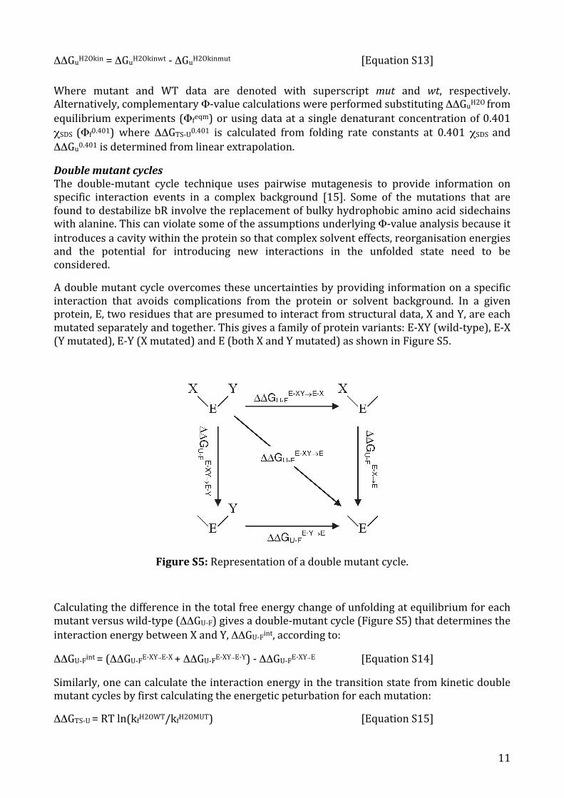
A double mutant cycle overcomes these uncertainties by providing information on a specific interaction that avoids complications from the protein or solvent background. In a given protein, E, two residues that are presumed to interact from structural data, X and Y, are each mutated separately and together. This gives a family of protein variants: E-‐XY (wild-‐type), E-‐X (Y mutated), E-‐Y (X mutated) and E (both X and Y mutated) as shown in Figure S5.

Figure S5: Representation of a double mutant cycle.

Calculating the difference in the total free energy change of unfolding at equilibrium for each mutant versus wild-‐type (ΔΔGU-‐F) gives a double-‐mutant cycle (Figure S5) that determines the interaction energy between X and Y, ΔΔGU-‐Fint, according to:

ΔΔGU-‐Fint = (ΔΔGU-‐FE-‐XY→E-‐X + ΔΔGU-‐FE-‐XY→E-‐Y) -‐ ΔΔGU-‐FE-‐XY→E [Equation S14]

Similarly, one can calculate the interaction energy in the transition state from kinetic double mutant cycles by first calculating the energetic peturbation for each mutation:

ΔΔGTS-‐U = RT ln(kfH2OWT/kfH2OMUT) [Equation S15]

12

And use this to calculate the coupling energy between X and Y according to:

ΔΔGTS-‐Uint = (ΔΔGTS-‐UE-‐XY→E-‐X + ΔΔGTS-‐UE-‐XY→E-‐Y) -‐ ΔΔGTS-‐UE-‐XY→E [Equation S16]

This allows us to calculate a Φ-‐value based on specific interaction energy, Φint, according to:

Φint = ΔΔGTS-‐Uint / ΔΔGU-‐Fint [Equation S17]

If Φint = 0, the native interaction energy is lost in the transition state and the two residues are no longer in contact. If Φint = 1 then the residues are in native-‐like contact in the transition state. The main advantage of Φint is that by isolating the interaction energy between X and Y errors from solvent and reorganization effects are much smaller and unfolded state effects cancel out; the method can thus unambiguously resolve whether mutations destabilise the protein by changes in solvent interactions as well as through the loss of structural interactions. Importantly, this method is well-‐suited to proteins with partially-‐structured unfolded states as for bR. Double mutant cycles have now been widely used to dissect the transition state structure of several small aqueous proteins [16, 17] and to analyse the contribution of electrostatic interactions to folding and stability [18, 19]. Additionally, double mutant Φ-‐values were used as a benchmark for computer simulations [20] of Barnase folding. With regard to integral membrane proteins, double mutant cycles have recently been used to examine the contributions of aromatic side-‐chains [21] and hydrogen bonding groups [22] to membrane protein folding and stability but have not yet been applied in mechanistic studies or in the context of transition state analysis.

SUPPLEMENTARY REFERENCES

1. Krebs, M.P., et al., Expression of the bacterioopsin gene in Halobacterium halobium using a multicopy plasmid. Proc. Natl. Acad. Sci. USA, 1991. 88(3): p. 859-‐863.

2. Cline, S.W. and F.W. Doolittle, Efficient transfection of the archaebacterium Halobacterium halobium. J. Bacteriol., 1987. 169(3): p. 1341-‐1344.

3. Oesterhelt, D. and W. Stoeckenius, Isolation of the cell membrane of Halobacterium halobium and its fractionation into red and purple membrane. Methods Enzymol., 1974. 31: p. 667-‐678.

4. Whitelegge, J.P., C.B. Gundersen, and K.Y. Faull, Electrospray-ionization mass spectroscopy of intact intrinsic membrane proteins. Protein Science, 1998. 7: p. 1423-‐1430.

5. Faham, S., et al., Side-chain contributions to membrane protein stability and structure. J. Mol. Biol., 2004. 335(1): p. 297-‐305.

6. Chen, G.Q. and E. Gouaux, Probing the folding and unfolding of wild-type and mutant forms of bacteriorhodopsin in micellar solutions: evaluation of reversible folding conditions. Biochemistry, 1999. 38: p. 15380-‐15387.

7. Curnow, P. and P.J. Booth, Combined kinetic and thermodynamic analysis of α-helical membrane protein unfolding. Proc. Natl. Acad. Sci. USA, 2007. 104(48): p. 18970-‐18975.

8. Brouillete, C.G., et al., Structure and thermal stability of monomeric bacteriorhodopsin in mixed phospholipid/detergent mixtures. Proteins: Structure, Function and Genetics, 1989. 5: p. 38-‐46.

9. Joh, N.H., et al., Modest stabilization by most hydrogen-bonded side-chain interactions in membrane proteins. Nature, 2008. 453(7199): p. 1266-‐1270.

10. Serrano, L., A. Matouschek, and A.R. Fersht, The folding of an enzyme. III. Structure of the transition state for unfolding of barnase analysed by a protein engineering procedure. J. Mol. Biol., 1992. 224(3): p. 805-‐818.

13

11. Clarke, J. and A.R. Fersht, Engineered disulfide bonds as probes of the folding pathway of barnase: increasing the stability of proteins against the rate of denaturation. Biochemistry, 1993. 32: p. 4322-‐4329.

12. Fersht, A.R., Structure and Mechanism in Protein Science. 1998, New York, NY, USA: W. H. Freeman and Co.

13. Booth, P.J., et al., Intermediates in the folding of the membrane protein bacteriorhodopsin. Nat. Struct. Biol., 1995. 2(2): p. 139-‐143.

14. Booth, P.J., A. Farooq, and S.L. Flitsch, Retinal binding during folding and assembly of the membrane protein bacteriorhodopsin. Biochemistry, 1996. 35: p. 5902-‐5909.

15. Horovitz, A., Double-mutant cycles: a powerful tool for analysing protein structure and function. Fold. Des., 1996. 1(6): p. R121-‐126.

16. Grantcharova, V.P., D.S. Riddle, and D. Baker, Long-range order in the src SH3 folding transition state. Proc. Natl. Acad. Sci. USA, 2000. 97(13): p. 7084-‐7089.

17. Horovitz, A., L. Serrano, and A.R. Fersht, COSMIC analysis of the major alpha-helix of barnase during folding. J. Mol. Biol., 1991. 219(1): p. 5-‐9.

18. Tissot, A.C., S. Vuilleumier, and A.R. Fersht, Importance of two buried salt bridges in the stability and folding pathway of barnase. Biochemistry, 1996. 35(21): p. 6786-‐6794.

19. Serrano, L., et al., Estimating the contribution of engineered surface electrostatic interactions to protein stability by using double mutant cycles. Biochemistry, 1990. 29(40): p. 9343-‐9352.

20. Salvatella, X., et al., Determination of the folding transition states of barnase by using ΦI-value-restrained simulations validated by double mutant ΦJ-values. Proc. Natl. Acad. Sci. USA, 2005. 102(35): p. 12389-‐12394.

21. Hong, H., et al., Role of aromatic side chains in the folding and thermodynamic stability of integral membrane proteins. J. Am. Chem. Soc., 2007. 129: p. 8320-‐8327.

22. HyunJoong Joh, N., et al., Modest stabilization by most hydrogen-bonded side-chain interactions in membrane proteins. Nature, 2008. 453(7199): p. 1266-‐1270.

curnow SI revised proofs - pnas.org · ! 3!! Figure, S3:!Relationship! between! equilibrium and!...

Documents

Transcript of curnow SI revised proofs - pnas.org · ! 3!! Figure, S3:!Relationship! between! equilibrium and!...